Primers • Tensorboard
TensorBoard
- TensorBoard is a great way to track and visualize neural network performance over time as it trains!
-
TensorBoard was built for TensorFlow, but can also be used with PyTorch using the TensorBoardX library.
-
Let’s walk through the AWS TensorBoard code and see it in action on an AWS instance. Instructions here. Make sure to perform steps 5 and 6 (opening a port in your AWS security settings, and setting up an SSH tunnel to your machine).
Running TensorBoard Locally
- We’ve also created a few Tensorflow 2/Keras examples that you can run on your local machine. These examples demonstrate how to show how to display loss curves, images, and figures like confusion matrices for the MNIST classification task on your local machine.
Setup
- You’ll need a couple of python packages to get started with these examples. Run these commands to create a virtual environment for this tutorial and start a TensorBoard server:
virtualenv -p python3 .venv
source .venv/bin/activate
pip install numpy matplotlib tensorflow tensorboard scikit-learn
tensorboard --logdir logs &
- Running
tensorboard --logdir logs &will create a directory calledlogswhere TensorBoard will store the metrics from your training runs and start a TensorBoard server as a background process. - Open the TensorBoard dashboard by going to
localhost:6006in your browser (or whichever port number your server is running on).
Plotting losses, accuracies, and weight distributions
- For this first example we’ll plot train and val loss and accuracy curves in addition to histograms of the weights of our network as it trains. To do this, we import the TensorBoard callback,
configure where it will store the training logs (we name this directory as a formatted string representing the current time), and pass this callback to
model.fit():
import datetime
import tensorflow as tf
from tensorflow.keras.datasets import mnist
from tensorflow.keras.models import Sequential
from tensorflow.keras.layers import Flatten, Dense, Dropout
from tensorflow.keras.callbacks import TensorBoard

(x_train, y_train), (x_test, y_test) = mnist.load_data()
x_train, x_test = x_train / 255.0, x_test / 255.0

model = Sequential([
    Flatten(input_shape=(28, 28)),
    Dense(512, activation='relu'),
    Dropout(0.2),
    Dense(10, activation='softmax')
])
model.compile(optimizer='adam',
              loss='sparse_categorical_crossentropy',
              metrics=['accuracy'])

time = datetime.datetime.now().strftime("%Y%m%d-%H%M%S")
log_dir = f"logs/{time}"
tensorboard = TensorBoard(log_dir=log_dir, histogram_freq=1) # added

model.fit(
    x=x_train,
    y=y_train,
    epochs=5,
    validation_data=(x_test, y_test),
    callbacks=[tensorboard]
    )
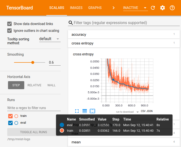
- We can see plots of the train and val losses and accuracies by navigating to the ‘Scalars’ tab of the TensorBoard dashboard at
localhost:6000in a browser.
-
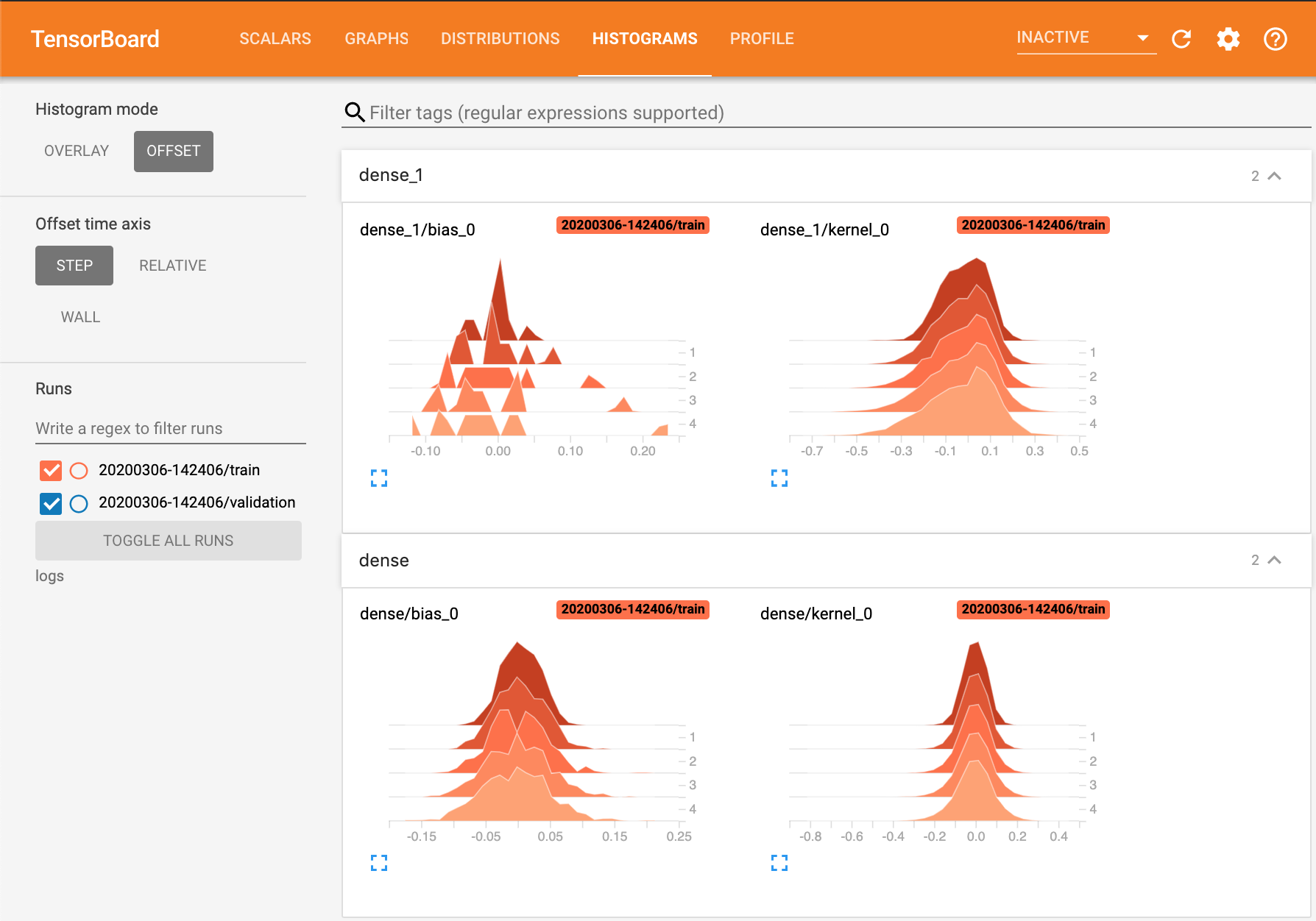
By setting
histogram_freq=1in the TensorBoard callback constructor, we can track the distributions of the weights in each layer at each epoch. -
The ‘Histograms’ tab shows histograms of the weights in each layer at each epoch.
Logging Images
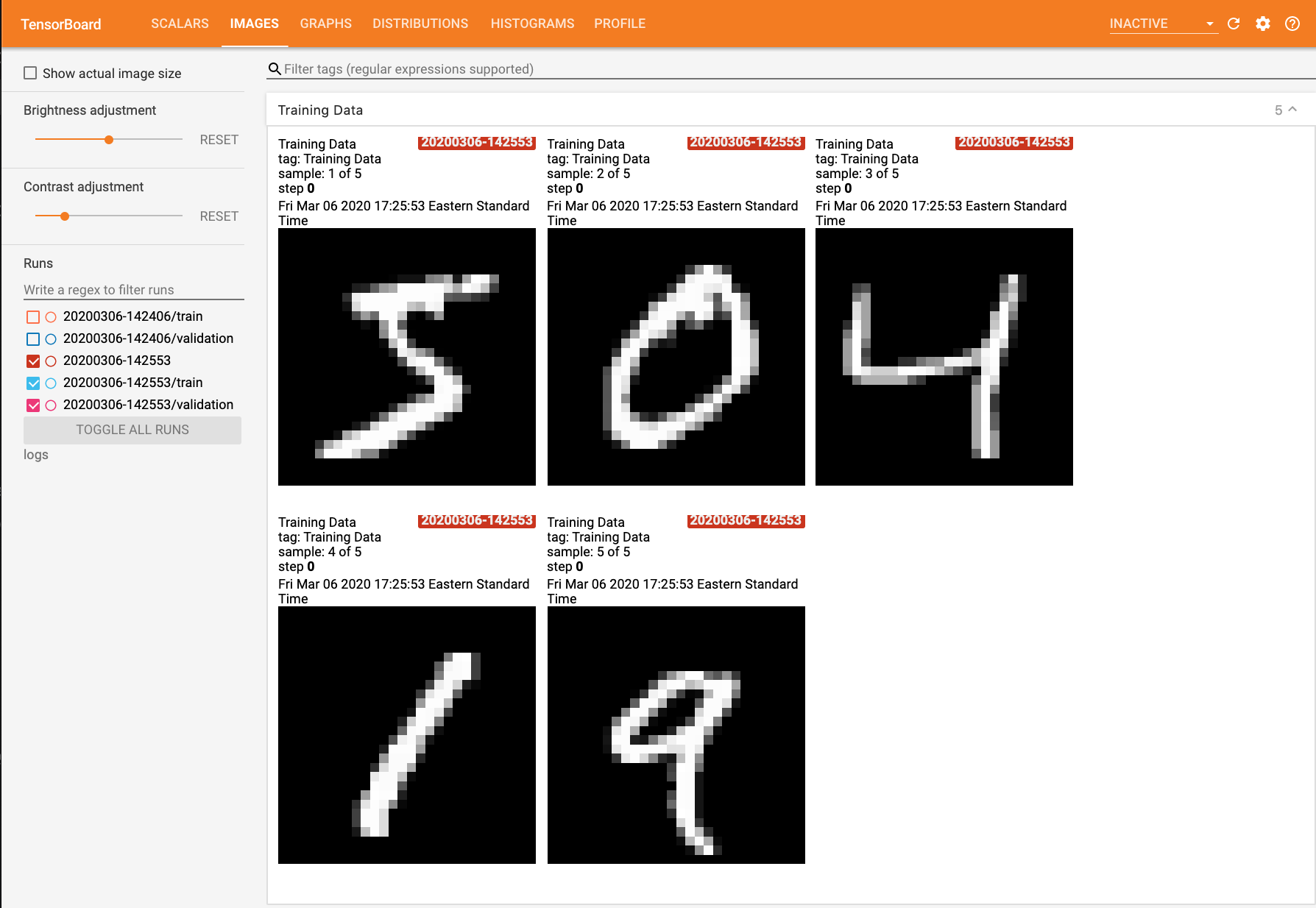
- This next example shows how to use
tf.summaryto log image data for visualization. Here we simply log the first five examples in the training set so that we can inspect them in the ‘Images’ tab of the TensorBoard dashboard.
import datetime
import tensorflow as tf
from tensorflow.keras.datasets import mnist
from tensorflow.keras.models import Sequential
from tensorflow.keras.layers import Flatten, Dense, Dropout
from tensorflow.keras.callbacks import TensorBoard

import matplotlib.pyplot as plt # added
import numpy as np # added
import sklearn.metrics # added

(x_train, y_train), (x_test, y_test) = mnist.load_data()
x_train, x_test = x_train / 255.0, x_test / 255.0

time = datetime.datetime.now().strftime("%Y%m%d-%H%M%S")
log_dir = f"logs/{time}"
tensorboard = TensorBoard(log_dir=log_dir, histogram_freq=1)

# Visualize image, added
images = np.reshape(x_train[0:5], (-1, 28, 28, 1)) # batch_size first
file_writer = tf.summary.create_file_writer(log_dir)
with file_writer.as_default():
	tf.summary.image("Training Data", images, max_outputs=5, step=0)

model = Sequential([
    Flatten(input_shape=(28, 28)),
    Dense(512, activation='relu'),
    Dropout(0.2),
    Dense(10, activation='softmax')
])
model.compile(optimizer='adam',
              loss='sparse_categorical_crossentropy',
              metrics=['accuracy'])

model.fit(
    x=x_train,
    y=y_train,
    epochs=5,
    validation_data=(x_test, y_test),
    callbacks=[tensorboard]
)
Custom Logging Callbacks
- The previous example showed how to log images from the training set at the beginning of training, but it would be more helpful to be able to log images and figures continusouly over the course of training.
- For example, if we were training a GAN, monitoring the loss curves of the generator and discriminator over time wouldn’t give much insight into the performance of the model, and it would be much more illuminating to be able to view samples generated over time to see if sample quality is improving.
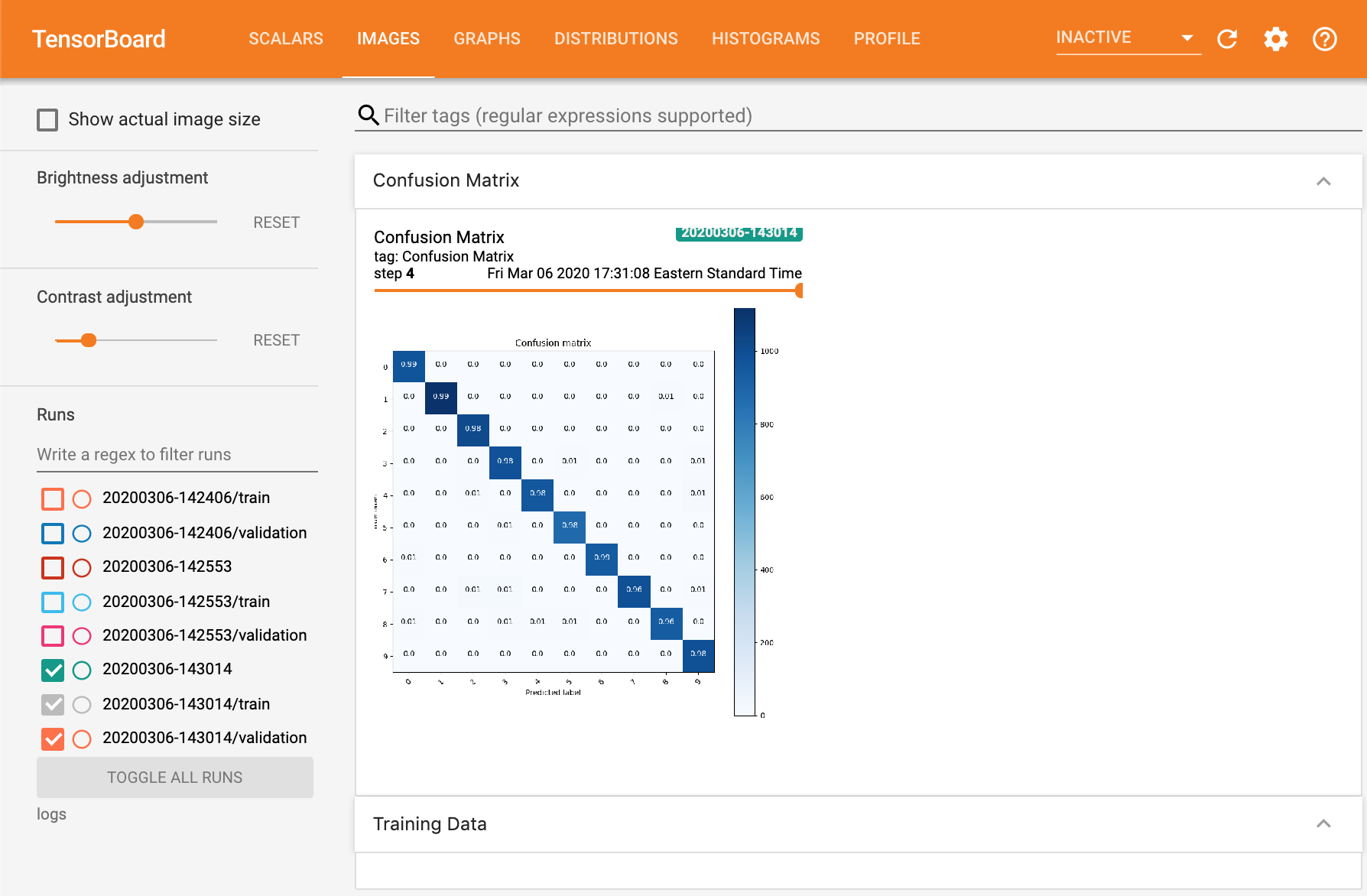
- Likewise, for a classification task like MNIST digit classification, being able to see the evolution of confusion matrices or ROC curves over time can give a better sense of model performance than a single number like accuracy. Here we show how to plot confusion matrices at the end of each epoch.
- We can define custom logging behavior that executes at fixed intervals during training using a
LambdaCallback. - In the code below, we define a function
log_confusion_matrixthat generates the model’s predictions on the val set and creates a confusion matrix image using thesklearn.metrics.confusion_matrix()function, and create a callback that plots the confusion matrix at the end of every epoch withcm_callback = LambdaCallback(on_epoch_end=log_confusion_matrix).
import datetime
import tensorflow as tf
from tensorflow.keras.datasets import mnist
from tensorflow.keras.models import Sequential
from tensorflow.keras.layers import Flatten, Dense, Dropout
from tensorflow.keras.callbacks import TensorBoard, LambdaCallback # added

import io # added
import itertools # added
import matplotlib.pyplot as plt
import numpy as np
import sklearn.metrics

# Added
def plot_to_image(fig):
	buf = io.BytesIO()
	plt.savefig(buf, format='png')
	plt.close(fig)
	buf.seek(0)
	img = tf.image.decode_png(buf.getvalue(), channels=4)
	img = tf.expand_dims(img, 0)
	return img

# Added
def plot_confusion_matrix(cm, class_names):
	figure = plt.figure(figsize=(8, 8))
	plt.imshow(cm, interpolation='nearest', cmap=plt.cm.Blues)
	plt.title("Confusion matrix")
	plt.colorbar()
	tick_marks = np.arange(len(class_names))
	plt.xticks(tick_marks, class_names, rotation=45)
	plt.yticks(tick_marks, class_names)

	cm = np.around(cm.astype('float') / cm.sum(axis=1)[:, np.newaxis], decimals=2)

	threshold = cm.max() / 2.
	for i, j in itertools.product(range(cm.shape[0]), range(cm.shape[1])):
		color = "white" if cm[i, j] > threshold else "black"
		plt.text(j, i, cm[i, j], horizontalalignment="center", color=color)

	plt.tight_layout()
	plt.ylabel('True label')
	plt.xlabel('Predicted label')
	return figure

(x_train, y_train), (x_test, y_test) = mnist.load_data()
x_train, x_test = x_train / 255.0, x_test / 255.0

time = datetime.datetime.now().strftime("%Y%m%d-%H%M%S")
log_dir = f"logs/{time}"
tensorboard = TensorBoard(log_dir=log_dir, histogram_freq=1)

# Added
file_writer = tf.summary.create_file_writer(log_dir)
def log_confusion_matrix(epoch, logs):
	test_pred_raw = model.predict(x_test)
	test_pred = np.argmax(test_pred_raw, axis=1)

	cm = sklearn.metrics.confusion_matrix(y_test, test_pred)
	figure = plot_confusion_matrix(cm, class_names=list(range(10)))
	cm_image = plot_to_image(figure)
	with file_writer.as_default():
		tf.summary.image("Confusion Matrix", cm_image, step=epoch)
cm_callback = LambdaCallback(on_epoch_end=log_confusion_matrix)

model = Sequential([
    Flatten(input_shape=(28, 28)),
    Dense(512, activation='relu'),
    Dropout(0.2),
    Dense(10, activation='softmax')
])
model.compile(optimizer='adam',
              loss='sparse_categorical_crossentropy',
              metrics=['accuracy'])

model.fit(
    x=x_train,
    y=y_train,
    epochs=5,
    validation_data=(x_test, y_test),
    callbacks=[tensorboard, cm_callback] # added
)
LambdaCallbacks allow us to view the history of confusion matrices summarizing our model’s performance on the val set over time:
References
Citation
If you found our work useful, please cite it as:
@article{Chadha2020DistilledTensorboard,
  title   = {Tensorboard},
  author  = {Chadha, Aman},
  journal = {Distilled AI},
  year    = {2020},
  note    = {\url{https://aman.ai}}
}