Primers • Support Vector Machines (SVM)
- Overview
- Key Concepts
- Loss Function: Hinge Loss
- Kernel / Polynomial Trick
- The Kernel Trick in SVMs
- Common Kernel Functions
- Advantages of the Kernel Trick
- Choosing the Right Kernel
- Applications
- Pros and Cons
- Example: SVM in Classification
- References
- Citation
Overview
- Support Vector Machines (SVMs) are a powerful supervised learning algorithm used for both classification and regression tasks. They are widely appreciated for their ability to handle high-dimensional data and robust performance, even in complex datasets.
- SVMs were first introduced by Vladimir Vapnik and Alexey Chervonenkis in 1963 as a binary classifier. The goal of SVM is to find the best hyperplane that separates data points of different classes in the feature space. For datasets that are not linearly separable, SVM employs kernel functions to map data into a higher-dimensional space where separation becomes feasible.
Key Concepts
Hyperplane
- A hyperplane is a decision boundary that separates data into different classes. In an \(n\)-dimensional space, the hyperplane is an \((n-1)\)-dimensional subspace.
Equation of a Hyperplane
\(\mathbf{w} \cdot \mathbf{x} + b = 0\)
- where:
- \(\mathbf{w}\): Weight vector (normal to the hyperplane)
- \(\mathbf{x}\): Feature vector
- \(b\): Bias term
- The goal is to maximize the margin between the hyperplane and the nearest data points of any class (support vectors).
Margin
- The margin is the distance between the hyperplane and the closest data points (support vectors) of either class. A larger margin generally leads to better generalization.
Functional Margin
\(y_i (\mathbf{w} \cdot \mathbf{x}_i + b) \geq 1\)
- where \(y_i \in \{-1, +1\}\): True label of the \(i\)-th data point.
Support Vectors
- Support vectors are the data points that lie closest to the hyperplane and influence its orientation and position. These points are critical in defining the margin.
Optimization Problem
- The optimization problem for a linear SVM is:
- Subject to:
- This is a convex optimization problem, solvable using techniques like Lagrange multipliers and quadratic programming.
Loss Function: Hinge Loss
- The hinge loss function is used to penalize misclassified points and points within the margin:
\(L = \sum_{i=1}^N \max(0, 1 - y_i (\mathbf{w} \cdot \mathbf{x}_i + b))\)
- where \(N\) is the total number of samples.
-
The objective function becomes:
\[\min_{\mathbf{w}, b} \frac{1}{2} \|\mathbf{w}\|^2 + C \sum_{i=1}^N \max(0, 1 - y_i (\mathbf{w} \cdot \mathbf{x}_i + b))\]- where \(C\) is a regularization parameter controlling the trade-off between maximizing the margin and minimizing the classification error.
Kernel / Polynomial Trick
Conceptual Overview
-
In classical machine learning, the goal of a classification task is to learn a function \(y = f(x; \theta)\), that is, to fit a model (or a curve) to the data in such a way that a decision boundary separates the classes — for instance, deciding whether to approve or reject loan applications.
-
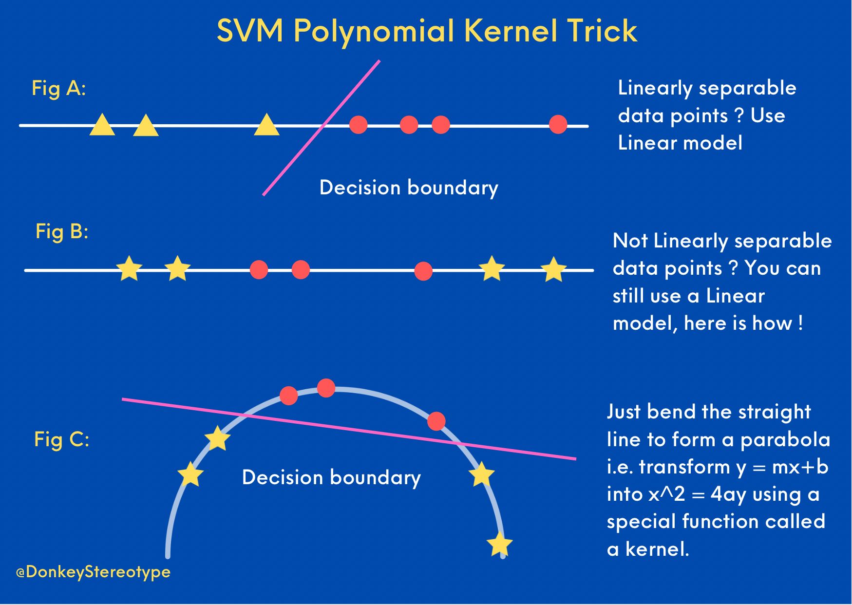
The figure below, adapted from Prithvi Da, visually summarizes different approaches to achieving separability in data.
Linear vs. Non-Linear Separability
-
Fig A: When data points are linearly separable, the problem is straightforward — algorithms such as logistic regression or a linear Support Vector Machine (SVM) can effectively fit a linear decision boundary.
-
Fig B: However, when the data points are not linearly separable, a simple linear boundary cannot adequately classify the samples. While neural networks are theoretically capable of learning any Borel measurable function, they may be excessive for small or tabular datasets.
-
Fig C: Instead, a simpler and elegant solution involves transforming the input space using a non-linear mapping. This transformation allows us to represent the same data in a higher-dimensional space where it becomes linearly separable. For example, transforming a line \(y = mx + c\) (a first-degree polynomial) into a parabola \(x^2 = 4ay\) (a second-degree polynomial) can make classification feasible in the higher-dimensional feature space.
-
This process of implicitly applying a non-linear transformation via a function known as a kernel forms the foundation of what is called the kernel trick. In essence, learning a linear model in a higher-dimensional feature space is equivalent to learning a non-linear model in the original space. In other words, by judiciously transforming the representation of the problem — figuratively “bending” it — one can often achieve a more effective and computationally elegant solution.
The Kernel Trick in SVMs
- The kernel trick is a cornerstone concept in SVMs that enables them to classify data that is not linearly separable in the original feature space. It achieves this by implicitly mapping data into a higher-dimensional feature space using kernel functions — without explicitly performing the transformation. This allows complex decision boundaries to be computed efficiently.
Why Use the Kernel Trick?
- For data that cannot be linearly separated in its original feature space, a simple hyperplane is insufficient. Instead of manually introducing additional dimensions, the kernel trick allows the SVM to compute the necessary separation in a higher-dimensional space using only inner products, greatly simplifying computation.
The Key Insight
- If \(\phi(\mathbf{x})\) represents the mapping from the input space to a higher-dimensional feature space, then the dot product in that space can be represented as a kernel function \(K\):
- This approach eliminates the need to explicitly compute \(\phi(\mathbf{x})\), making training and inference computationally efficient.
Common Kernel Functions
Linear Kernel
\[K(\mathbf{x}_i, \mathbf{x}_j) = \mathbf{x}_i^\top \mathbf{x}_j\]- Suitable for linearly separable data.
- No explicit transformation is performed.
Polynomial Kernel
\[K(\mathbf{x}_i, \mathbf{x}_j) = (\mathbf{x}_i^\top \mathbf{x}_j + c)^d\]- \(c\): A constant controlling flexibility.
- \(d\): The degree of the polynomial.
- Captures polynomial relationships between features and mirrors the principle illustrated in Fig C above, where a polynomial transformation enhances separability.
Radial Basis Function (RBF) or Gaussian Kernel
\[K(\mathbf{x}_i, \mathbf{x}_j) = \exp\left(-\gamma |\mathbf{x}_i - \mathbf{x}_j|^2\right)\]- $$\gammah: Controls the influence of each data point.
- Maps data into an infinite-dimensional space.
- Highly effective for complex, non-linear relationships.
Sigmoid Kernel
\[K(\mathbf{x}_i, \mathbf{x}_j) = \tanh(\alpha \mathbf{x}_i^\top \mathbf{x}_j + c)\]- Inspired by neural network activation functions.
- Parameters \(\alpha\) and \(c\) govern the decision boundary’s shape.
- Can approximate neural network behavior under specific parameter settings.
Advantages of the Kernel Trick
-
Efficiency: Avoids explicit computation of the high-dimensional feature space, thereby reducing computational overhead.
-
Flexibility: Allows SVMs to handle both linear and highly non-linear datasets effectively.
-
Scalability: Can manage very high-dimensional data without significantly increasing memory requirements.
Choosing the Right Kernel
- Linear Kernel: Best for linearly separable data or datasets with many features.
- Polynomial Kernel: Suitable when feature interactions up to a specific degree are significant.
- RBF Kernel: Often the default choice for non-linear datasets due to its flexibility.
- Sigmoid Kernel: Use cautiously; its performance can vary depending on data characteristics.
Applications
- Classification Tasks:
- Handwriting recognition (e.g., MNIST dataset)
- Text categorization (e.g., spam filtering)
- Bioinformatics (e.g., cancer detection)
- Regression Tasks:
- Predicting real estate prices.
- Financial forecasting.
- Outlier Detection:
- Detecting anomalies in time series data.
- Fraud detection in financial systems.
Pros and Cons
Pros
-
Effective in High Dimensions: SVM works well in datasets with a large number of features.
-
Robust to Overfitting: Particularly effective in scenarios with a clear margin of separation.
-
Versatility: Through the use of kernels, SVM can handle nonlinear relationships.
-
Sparse Solutions: The model depends only on support vectors, reducing computation.
Cons
-
Scalability: SVM is computationally expensive for large datasets due to quadratic programming.
-
Choice of Kernel: The performance heavily depends on the choice of the kernel function and its parameters.
-
Interpretability: Nonlinear SVM models are harder to interpret than linear models.
-
Memory-Intensive: Storing support vectors for large datasets can be memory-intensive.
Example: SVM in Classification
Given Dataset
- \[X = \{ \mathbf{x}_1, \mathbf{x}_2, ..., \mathbf{x}_N \}\]
- Labels: \(y_i \in \{-1, +1\}\)
Model
-
Using the RBF kernel: \(K(\mathbf{x}_i, \mathbf{x}_j) = \exp\left(-\gamma \|\mathbf{x}_i - \mathbf{x}_j\|^2\right)\)
-
Optimization: \(\min_{\mathbf{w}, b} \frac{1}{2} \|\mathbf{w}\|^2 + C \sum_{i=1}^N \max(0, 1 - y_i (\mathbf{w} \cdot \mathbf{x}_i + b))\)
-
After training, for a new point \(\mathbf{x}_{\text{new}}\):
\(f(\mathbf{x}_{\text{new}}) = \text{sign} \left\)\sum_{i=1}^N \alpha_i y_i K(\mathbf{x}i, \mathbf{x}{\text{new}}) + b \right) $$
- where \(\alpha_i\) are the Lagrange multipliers obtained during optimization.
References
Citation
If you found our work useful, please cite it as:
@article{Chadha2020DistilledSVM,
  title   = {Support Vector Machines},
  author  = {Chadha, Aman},
  journal = {Distilled AI},
  year    = {2020},
  note    = {\url{https://aman.ai}}
}