Primers • State Space Models
- Overview
- From Dynamical Systems to Neural Sequence Models
- Continuous-Time State Space Models
- The State as Compressed Memory
- HiPPO: Turning State into a Principled Memory
- Discretizing the Continuous System
- Recurrence: The Streaming View
- Convolution: The Parallel Training View
- Why Linear SSMs Can Still Form Nonlinear Neural Networks
- SISO, MIMO, and Channel Structure
- Diagonal State Matrices
- Stability and Memory Timescales
- The Three Computational Views of an SSM
- The Long-Memory Problem and HiPPO
- Why Long-Term Memory Is Difficult
- Memory as Online Function Approximation
- The Measure Determines What Memory Means
- From Projection Coefficients to a State Space Model
- Why Orthogonal Polynomials
- Translated Legendre Memory
- Exponentially Decaying Memory
- HiPPO-LegS: Scaling the Window with Time
- Timescale Equivariance
- HiPPO and Gating
- Computational Complexity of HiPPO-LegS
- Gradient Flow
- Approximation Error
- From HiPPO to S4
- Structured State Space Models: S4
- From HiPPO Memory to a Practical Sequence Model
- Why Not Simply Diagonalize the State Matrix?
- Normal Plus Low-Rank Structure
- From NPLR to DPLR
- Why the Low-Rank Term Cannot Simply Be Ignored
- The SSM Generating Function
- Bilinear Discretization
- The Woodbury Identity
- From the Resolvent to a Cauchy Kernel
- Recovering the Kernel with the FFT
- Training as a Global Convolution
- Inference as a Recurrence
- The Deep S4 Layer
- Trainable Parameters
- Initialization Matters
- Numerical Stability
- Why Complex Numbers Appear
- S4 as a Global Convolution
- What the Learned Kernels Look Like
- Long Range Arena
- Computational Profile
- What S4 Solved
- What S4 Did Not Solve
- Simplifying Structured SSMs
- Why Simplify S4?
- Diagonal State Space Models
- DSS: The First Major Diagonal Simplification
- Why Expressivity Alone Is Not Enough
- S4D: S4 Without the Low-Rank Correction
- S4D and the Vandermonde View
- Stable Eigenvalue Parameterization
- S4D-LegS
- S4D-Inv
- S4D-Lin
- Initialization Is Still Critical
- What S4D Established
- From Convolution Back to Recurrence
- S5: One Multi-Input, Multi-Output SSM
- SISO Versus MIMO
- Parallel Associative Scan
- A Simple View of the Scan
- Why Diagonal Structure Matters for the Scan
- S5 Discretization
- Connecting S5 Back to S4
- HiPPO-N Initialization in S5
- Conjugate Symmetry
- The S5 Layer
- Why Scans Matter Beyond S5
- S4, S4D, and S5 as a Progression
- What Was Gained and What Was Lost
- SSMs for Language Modeling Before Mamba
- The Language Modeling Gap
- Synthetic Tasks as Architectural Diagnostics
- Remembering Versus Retrieving
- Inspiration from Linear Attention
- The H3 Layer
- The Shift SSM
- Why the Shift Operation Helps
- The Diagonal SSM
- Multiplicative Interaction
- How H3 Implements Associative Recall
- Why It Is Called H3
- Closing the Perplexity Gap
- A Small Amount of Attention Still Helps
- Scaling H3
- The Hardware Problem
- FlashConv
- Kernel Fusion
- Block FFT
- State Passing for Long Sequences
- FlashConv Performance
- H3’s Relationship to Attention
- What H3 Revealed About SSMs
- From H3 to Mamba
- Mamba and Selective State Space Models
- The Selection Problem
- Why Selection Matters
- Selective Copying
- Induction Heads
- From S4 to S6
- Input-Dependent Parameters
- Discretizing the Selective SSM
- Interpreting the Three Selective Parameters
- The Special Role of the Step Size
- Connection to Gated RNNs
- State Expansion
- Why Selection Breaks Convolution
- Returning to the Recurrent View
- The Hardware-Aware Selective Scan
- HBM and SRAM
- Kernel Fusion
- Chunking Long Sequences
- Recomputation Instead of Storing States
- Selective Scan as Algorithm-Architecture Co-Design
- The Mamba Block
- Why the Short Convolution Remains
- Expansion Factor
- No Attention and No Separate MLP
- Training Complexity
- Autoregressive Inference
- No KV Cache
- Selective Scan Performance
- Language Modeling Scaling
- Length Generalization
- Beyond Language
- Selection Versus Architectural Gating
- Mamba as a Learned Compression Mechanism
- The Fundamental Tradeoff
- What Mamba Changed
- Mamba-2 and Structured State Space Duality
- From Mamba to Mamba-2
- Three Views of Sequence Modeling
- SSMs as Sequence-to-Sequence Matrices
- Semiseparable Matrices
- Why Structured Matrices Matter
- The Scalar-Identity Restriction
- From SSM to Attention
- The Semiseparable Mask
- A Learned Relative Position Mechanism
- Connection to Linear Attention
- Tensor Contraction View
- Structured Masked Attention
- The Important Limitation
- Linear and Quadratic Modes
- Why Pure Recurrence Is Not Always Fast
- Block Decomposition
- Diagonal Blocks in Attention Mode
- Off-Diagonal Blocks in Recurrent Mode
- The Best of Both Computational Modes
- SSD Complexity
- Larger State Dimensions
- From SISO to Multi-Value State Spaces
- Multi-Value Attention Analogy
- The Mamba-2 Block
- Why Parallel Projection Helps
- Additional Normalization
- Tensor Parallelism
- SSD Versus Selective Scan
- Speed Relative to Mamba
- Simpler Implementation
- Mamba-2 Scaling
- Multi-Query Associative Recall
- State Size Versus Context Size
- Why Attention Still Differs
- SSD as a Bridge Between Research Traditions
- A New View of Sequence Mixers
- The Broader Structured Masked Attention Space
- From Mamba to Mamba-2
- What Mamba-2 Changed
- Mamba-3 and Inference-First SSM Design
- From Training Efficiency to Inference Efficiency
- Why Mamba-2 Leaves Room for Improvement
- An Inference-First Objective
- Arithmetic Intensity
- Returning to the Continuous-Time SSM
- Exponential-Euler Discretization
- The Limitation of Euler Approximation
- Exponential-Trapezoidal Discretization
- Why the Third Term Matters
- Euler as a Special Case
- A More Expressive Structured Mask
- Removing the External Short Convolution
- The State-Tracking Problem
- Why Real Decay Is Restrictive
- Complex-Valued State Transitions
- State Tracking as Rotation
- Connection to RoPE
- Data-Dependent Complex Dynamics
- Why Complex Dynamics Are an SSM-Native Extension
- SISO State Spaces
- Multi-Input Multi-Output State Spaces
- Why MIMO Helps Decode Efficiency
- More Compute Without Proportional Latency
- Parameter-Efficient MIMO
- The Mamba-3 Block
- BC Normalization
- Removing the Post-Gate Normalization
- Biases in the Write and Read Projections
- A More SSM-Centric Architecture
- State Tracking
- Retrieval
- Language Modeling
- Perplexity Improvements
- Better Use of State Capacity
- SISO Versus MIMO Under Fixed Inference Cost
- Context-Length Extrapolation
- Decode Kernels
- Prefill Versus Decode
- The Cost of Mamba-3’s Added Expressivity
- Mamba-1, Mamba-2, and Mamba-3
- The Evolution of the Recurrence
- Revisiting the Role of Discretization
- Revisiting Complex Numbers
- Revisiting MIMO
- The Performance-Efficiency Frontier
- What Mamba-3 Changed
- Hybrid SSM-Attention Architectures
- Why Hybridize SSMs and Attention?
- Compressed Memory Versus Explicit Memory
- Why a Small Amount of Attention Can Matter
- The Retrieval Bottleneck
- Griffin
- Hawk and RG-LRU
- Why Local Attention?
- Jamba
- Attention-to-Mamba Ratio
- Jamba Blocks
- Adding Mixture of Experts
- Long Context in Jamba
- Why Jamba’s Attention Layers Matter
- In-Context Learning and Induction
- Zamba
- Shared Attention
- Parameter Sharing Versus Activation Sharing
- Spending FLOPs Without Spending Parameters
- Taipan
- Selective Attention
- Layer Sparsity Versus Token Sparsity
- Why Token Selection Makes Sense
- Nemotron-H
- Nemotron-H Layer Allocation
- Nemotron-H-8B
- Nemotron-H-56B
- Why Evenly Disperse Attention?
- Attention as a Memory Refresh
- KV-Cache Economics
- Why This Matters for Long Generation
- Inference-Time Scaling
- Nemotron-H Throughput
- A Spectrum of Hybrid Designs
- Three Axes of Attention Sparsity
- Hybridization as Conditional Memory Access
- Attention as an Exception Path
- Why Not Eliminate Attention Entirely?
- Why Not Use Attention Everywhere?
- Attention and Recurrence as Complementary Operations
- Hybrid Models and In-Context Learning
- Hybrid Models and Reasoning
- Static Versus Dynamic Hybridization
- Hybridization and MoE
- The Emerging Architectural Pattern
- A General Hybrid Sequence Model
- The Efficiency Frontier
- From Pure Architectures to Memory Systems
- What Hybrid Architectures Teach Us
- Recall, Memory, and the Limits of Fixed-State Models
- Recall Is Different From Long-Range Dependency
- Associative Recall
- Why Attention Is Naturally Suited to Recall
- Recall in a Recurrent Model
- The Compression Bottleneck
- Zoology
- Recall-Intensive Tokens
- Model Scale Does Not Automatically Solve Recall
- Synthetic Recall Can Be Misleading
- Multi-Query Associative Recall
- Why MQAR Is Harder
- Attention and MQAR
- Mamba Changes the Recall Frontier
- Selective Copying
- Induction Heads
- The Recall-Memory Tradeoff
- State Size as an Inference Resource
- A Pareto Frontier
- Why Architecture Still Matters at Fixed State Size
- Information Must Go Somewhere
- Lower Bounds on Recall Memory
- Continuous States Do Not Give Infinite Practical Memory
- Memory Capacity Versus Model Capacity
- Exact Recall Versus Approximate Recall
- Natural Language Is Highly Compressible
- Recall Is Query-Dependent
- Selection Helps but Does Not Remove the Problem
- Forgetting Is Necessary
- Linear Attention as Fixed-State Associative Memory
- Based
- Why Linear Attention Alone Is Not Enough
- Why Sliding-Window Attention Alone Is Not Enough
- Based as a Two-Tier Memory
- Dialing the Memory Budget
- Recall on Real Language Tasks
- Based Versus Other Subquadratic Models
- Recall and Throughput Are Coupled
- Hardware Changes the Frontier
- The Throughput-Recall Frontier
- Recall Versus State Tracking
- Sufficient Statistics
- When Fixed-State Models Are Ideal
- When Explicit Memory Is Valuable
- Memory as an Architectural Budget
- The Memory Hierarchy View
- Recall as a Systems Problem
- No Free Recall
- A More Precise View of the SSM Limitation
- The Emerging Design Principle
- From Recall Limits to Implementation
- Training and Implementation
- Why SSM Implementation Is Unusual
- Training and Inference Need Different Algorithms
- S4 Training Through Convolution
- FFT Convolution
- Padding for FFT Convolution
- S4 Kernel Generation
- S4 Recurrent Inference
- Diagonal SSM Implementation
- Why Initialization Is Part of the Implementation
- Learnable Timescales
- S5 and Parallel Associative Scan
- Why Associativity Matters
- A Conceptual Scan Implementation
- Mamba Breaks the Convolution Shortcut
- The Naive Selective Scan
- Arithmetic Is Not Always the Bottleneck
- HBM and SRAM
- Hardware-Aware Selective Scan
- Kernel Fusion
- Memory-Traffic Reduction
- Chunking Long Sequences
- Recomputation During Backpropagation
- Recomputation Is Not Ordinary Checkpointing
- Memory Complexity During Training
- Tensor Layout Matters
- Avoiding Materialized Transposes
- Mamba Block Fusion
- Causal Convolution
- Mamba Inference State
- Prefill Versus Decode
- Mamba-2 Changes the Training Primitive
- SSD Chunking
- Why Local Quadratic Computation Can Be Faster
- SSD Block Decomposition
- Matrix Multiplication as a Systems Primitive
- Choosing Chunk Size
- Mamba-2 Parallel Projections
- Larger States Become Practical
- Mamba-2 Inference
- Normalization
- Mamba-2 Internal Normalization
- Residual Connections
- Mixed Precision
- Why BF16 Is Often Attractive
- Complex-Valued States
- Conjugate Symmetry
- Mamba-3 Returns Attention to Decode Efficiency
- Mamba-3 SISO Decode
- Mamba-3 MIMO and Arithmetic Intensity
- Mamba-3 Prefill and Decode Tradeoff
- Separate Prefill and Decode Kernels
- Inference State Caching
- Continuous Batching
- Prompt Prefill Still Matters
- State Serialization
- Sequence Packing
- Variable-Length Batches
- Distributed Training
- Tensor Parallelism
- Sequence Parallelism Is More Subtle
- Hybrid Models
- Grouped-Query Attention in Hybrids
- Initialization Checklist
- Gradient Stability
- Gradient Clipping
- Learning Rates for SSM Parameters
- Weight Decay
- Reference Implementation Versus Production Kernel
- Numerical Equivalence Tests
- Chunk-Boundary Tests
- Prefill-Decode Equivalence
- Benchmark the Right Quantities
- Benchmark at Realistic Batch Sizes
- Benchmark Across Context Length
- FLOPs Are Not Enough
- Roofline Perspective
- Common Implementation Failure: Python Loops
- Common Implementation Failure: Materializing Expanded States
- Common Implementation Failure: Ignoring Decode State
- Common Implementation Failure: Reset Bugs
- Common Implementation Failure: Incorrect Causality
- Common Implementation Failure: Comparing Unoptimized Baselines
- A Minimal SSM Training Skeleton
- A Minimal Recurrent Serving Interface
- State Allocation Should Be Explicit
- Training-Time Memory Accounting
- Production Implementation Strategy
- The Broader Systems Lesson
- Algorithm-Architecture-Hardware Co-Design
- Complexity and Systems Analysis
- Why Asymptotic Complexity Is Not Enough
- Notation
- Full Self-Attention
- FlashAttention Changes Memory Traffic, Not the Mathematics
- Attention Prefill
- Attention Decode
- KV-Cache Growth
- Multi-Query and Grouped-Query Attention
- Sliding-Window Attention
- The Limitation of Sliding Windows
- Classical Recurrent Networks
- Why SSMs Differ from Generic RNNs
- S4 Complexity
- S4 Decode
- S5 Complexity
- Mamba Complexity
- Mamba Decode
- Constant Memory Does Not Mean Constant Total Cost
- Mamba-2 Complexity
- SSD Versus Selective Scan
- Why Chunking Helps SSD
- Mamba-3 Complexity
- SISO Versus MIMO Decode
- Linear Attention
- Linear Attention and SSMs
- Gated Linear Recurrences
- The State-Size Dimension
- Attention Stores History Explicitly
- SSMs Compress History
- Memory Bandwidth During Decode
- Arithmetic Intensity
- Why Attention Can Be Fast Despite Quadratic FLOPs
- Roofline Interpretation
- Kernel Launch Overhead
- Prefill Parallelism
- Decode Parallelism
- Batch Size as a Systems Variable
- Continuous Batching
- Paged KV Caches Narrow the Gap
- Beam Search
- Speculative Decoding
- Prefix Sharing
- Context Extension
- Long-Context Extrapolation
- Hybrid Complexity
- Hybrid KV-Cache Memory
- Nemotron-H as a Systems Example
- Local Attention Hybrids
- Shared Attention Modules
- Mixture-of-Experts Hybrids
- Communication Can Dominate Distributed Training
- SSM Tensor Parallelism
- Attention Tensor Parallelism
- Sequence Parallelism
- Pipeline Parallelism
- Training Activation Memory
- Checkpointing
- Training Throughput
- Prefill Latency
- Time to First Token
- Inter-Token Latency
- Throughput Versus Latency
- Energy
- A Simplified Complexity Comparison
- Capability per Byte of Persistent Memory
- Capability per Unit of Latency
- The Crossover Point Is Workload Dependent
- Short Contexts
- Long Prompts
- Long Generation
- High Concurrency
- Retrieval-Heavy Workloads
- Streaming Workloads
- Edge Devices
- Training Hardware Versus Serving Hardware
- Training Once, Serving Many Times
- Why Hybrids Are a Natural Endpoint
- The Systems Evolution of SSMs
- Practical Interpretation of “Linear-Time”
- Practical Interpretation of “Constant-Memory”
- The Central Tradeoff
- Applications Beyond Language
- Why SSMs Generalize Beyond Text
- The General Sequence Modeling View
- Continuous Signals Are a Natural Starting Point
- Audio and Speech
- S4 and Long Audio
- SaShiMi and Audio Generation
- Hierarchical Audio Modeling
- Speech Recognition
- Streaming Speech
- Speech and Selectivity
- Genomics
- Why Genomics Is Difficult for Full Attention
- HyenaDNA
- Mamba for DNA
- DNA Is Not Simply Text with Four Tokens
- Time Series
- Classical State Estimation
- Long-Horizon Forecasting
- Irregularly Sampled Data
- S5 and Variable Timescales
- Event Streams
- Vision
- Why Vision Needs Special Treatment
- Vision Mamba
- VMamba and Two-Dimensional Scanning
- Selective Scan in Two Dimensions
- Vision Complexity
- Locality Still Matters in Vision
- Hierarchical Vision
- Video
- Temporal Recurrence in Video
- Spatial and Temporal State
- Long Video Understanding
- Robotics
- Partial Observability
- Action-Conditioned State Transitions
- SSMs as Policy Memory
- Control Frequency
- World Models
- SSMs and Latent Dynamics
- Embodied Multimodal Agents
- A Multirate Architecture
- Scientific Data
- Medical Signals
- Sensor Networks
- Anomaly Detection
- Financial Event Streams
- Graphs and Spatial Systems
- Multidimensional SSMs
- Causal Versus Bidirectional Applications
- Offline Sequence Modeling
- Streaming Sequence Modeling
- Multiscale State
- Resolution Versus Context
- Compression Before the Model Versus Inside the Model
- The Cost of Compression
- When SSMs Are Particularly Natural
- When Attention Remains Valuable
- Hybrid Memory Beyond Language
- SSMs as Part of Larger Systems
- A Cross-Domain Perspective
- The Broader Significance of SSMs
- Practical Model Selection
- Architecture Selection Is a Workload Decision
- Start with the Memory Requirement
- When Full Attention Is the Natural Baseline
- Do Not Replace Attention Merely Because the Sequence Is Long
- When Sliding-Window Attention Is Enough
- When Linear Attention Is Attractive
- When an SSM Is the Natural Choice
- When S4 Is Still Useful
- When S4D or S5 Is Preferable
- When Mamba Is a Good Choice
- When Mamba-2 Is Preferable
- When Mamba-3 Is Preferable
- Choosing Between Mamba-3 SISO and MIMO
- When a Pure SSM Is Risky
- Recall Should Be Benchmarked Directly
- MQAR as an Architecture Diagnostic
- State Size Is a Hyperparameter, Not a Constant of Nature
- Recall Versus State Size
- When Hybrid Architectures Are the Safer Choice
- Jamba as a Hybrid Design Point
- What Jamba’s Ablations Suggest
- Zamba as a Shared-Attention Design
- Griffin and Local Attention
- Based as a Two-Tier Memory Architecture
- Nemotron-H as a Sparse-Attention Design Point
- Choosing the Attention Fraction
- Where to Put Attention Layers
- Attention Does Not Need to Be Global
- Model Selection for Long-Context Language Modeling
- Long Prompt, Short Generation
- Short Prompt, Long Generation
- Long Prompt, Long Generation
- Retrieval-Augmented Systems Change the Decision
- External Memory and Recurrent State Are Complementary
- Model Selection for Agents
- A Memory Hierarchy for Agents
- Model Selection for Streaming Applications
- Model Selection for Audio
- Model Selection for Genomics
- Model Selection for Vision
- Model Selection for Video
- Model Selection for Robotics
- Training Cost Versus Serving Cost
- Prefill-Dominated Versus Decode-Dominated Serving
- Latency-Sensitive Applications
- Throughput-Sensitive Applications
- Memory-Constrained Deployment
- Edge Deployment
- Kernel Availability Should Influence Architecture Choice
- Model Ecosystem Matters
- Benchmark the Actual Deployment Distribution
- Benchmark Quality at Equal Compute
- Benchmark Quality at Equal Parameter Count
- Benchmark at Equal Latency
- Benchmark at Equal Memory
- Benchmark the Pareto Frontier
- Include Short and Long Contexts
- Include Multiple Batch Sizes
- Evaluate State Capacity Directly
- Evaluate Attention Fraction Directly
- Evaluate Attention Placement
- Evaluate Local Versus Global Attention
- Evaluate Long-Context Recall Separately from Perplexity
- Evaluate Extrapolation
- Evaluate Streaming Stability
- Evaluate Reset Semantics
- Evaluate Prefill-Decode Equivalence
- Evaluate Chunk-Boundary Invariance
- A Practical Decision Matrix
- A Practical Architecture Search Strategy
- A Conservative Hybrid Starting Point
- A Pure Recurrent Starting Point
- Avoid Architecture Decisions from FLOPs Alone
- Avoid Architecture Decisions from Asymptotics Alone
- Avoid Architecture Decisions from One Benchmark
- Avoid Treating “Long Context” as One Capability
- Avoid Treating Constant State as Free Memory
- Avoid Treating Attention as Inherently Inefficient
- Avoid Treating SSMs as Merely Efficient RNNs
- A Research-Oriented Selection Framework
- A Systems-Oriented Selection Framework
- A Capability-Oriented Selection Framework
- A Useful Three-Axis View
- The Emerging Design Space
- Final Selection Principles
- Closing Perspective
- FAQ
- Models
- Related Papers
- Efficiently Modeling Long Sequences with Structured State Spaces
- Mamba: Linear-Time Sequence Modeling with Selective State Spaces
- MambaByte: Token-free Selective State Space Model
- Scalable Diffusion Models with State Space Backbone
- Cobra: Extending Mamba to Multi-Modal Large Language Model for Efficient Inference
- SAMBA: Simple Hybrid State Space Models for Efficient Unlimited Context Language Modeling
- Further Reading
- References
- State Space Model and HiPPO foundations
- S4 and structured State Space Models
- State Space Models for language modeling
- Mamba and selective State Space Models
- Structured State Space Duality and Mamba-2
- Mamba-3 and inference-oriented SSMs
- Hybrid Mamba-attention architectures
- Recall, associative memory, and recurrent-state capacity
- Linear attention and recurrent alternatives
- Attention systems and IO-aware sequence processing
- Vision State Space Models
- Video State Space Models
- Genomics and biological sequence modeling
- Reinforcement learning, control, and sequential decision making
- Core implementation and explanatory resources
- Citation
Overview
-
State Space Models (SSMs) are sequence models built around a compact latent state that evolves over time. Instead of explicitly comparing every token with every earlier token, as self-attention does, an SSM repeatedly updates a fixed-size hidden state and produces outputs from that state. In its classical continuous-time form, a linear state-space system can be written as
\[\frac{d h(t)}{dt} = A h(t) + B x(t)\] \[y(t) = C h(t) + D x(t)\] -
where \(x(t)\) is the input, \(h(t)\) is the latent state, \(y(t)\) is the output, and \(A\), \(B\), \(C\), and \(D\) determine how information enters, evolves within, and leaves the state. After discretization, this becomes a recurrence of the form
\[h_t = \bar{A}h_{t-1} + \bar{B}x_t\] \[y_t = Ch_t + Dx_t\] -
The central appeal is that the model can process an arbitrarily long sequence while carrying forward a state whose size does not grow with sequence length. This gives SSMs a natural recurrent interpretation and makes them attractive for streaming and long-context inference.
-
Modern neural SSMs turn this classical dynamical-systems abstraction into a trainable sequence-modeling primitive. The key challenge is not merely writing down the recurrence, but making it simultaneously capable of preserving information over long horizons, trainable in parallel on modern accelerators, expressive enough for language and other discrete modalities, and efficient during autoregressive inference.
-
The modern line of work began to address these requirements through increasingly structured parameterizations. HiPPO: Recurrent Memory with Optimal Polynomial Projections by Gu et al. (2020) introduced a principled mechanism for continuously compressing a signal’s history into a fixed-dimensional state using projections onto orthogonal polynomial bases. HiPPO provided the mathematical memory mechanism that later structured SSMs built upon.
-
Efficiently Modeling Long Sequences with Structured State Spaces by Gu et al. (2021) introduced S4, which transformed this foundation into a practical deep sequence layer by imposing structure on the state matrix and exploiting the equivalence between recurrent and convolutional views of an SSM. S4 demonstrated that carefully structured state spaces could model dependencies over tens of thousands of steps while remaining computationally practical.
-
The broader progression from HiPPO to S4, simplified SSMs, Mamba, Mamba-2, and newer hybrid architectures can therefore be understood as an effort to answer three recurring questions: how should information be compressed into a finite state, how can that state be updated efficiently, and how can the model decide which information should be retained or discarded?
Why State Space Models Matter
-
Transformers obtain their expressive power largely through content-dependent self-attention. Given a sequence, each token can directly retrieve information from other tokens through query-key similarity. This provides unusually strong associative recall, but it also introduces scaling costs.
-
For a sequence of length \(L\), standard full self-attention constructs an \(L \times L\) attention matrix during parallel processing. Training-time attention therefore has quadratic dependence on sequence length in its conventional form. During autoregressive inference with a KV cache, the model avoids recomputing earlier keys and values, but each newly generated token still attends over an increasingly large cache. Consequently, attention computation per generated token grows with context length, and KV-cache memory also grows with context length.
-
An SSM instead compresses the past into a recurrent state
\[h_t = f(h_{t-1}, x_t)\] -
and computes the output from that state
\[y_t = g(h_t, x_t)\] -
For a fixed state size, the amount of persistent recurrent state need not increase with sequence length. Autoregressive inference can therefore operate with constant recurrent-state memory with respect to context length and constant per-token state-update complexity with respect to context length.
-
This difference makes SSMs especially attractive when sequences become very long or when inference must be streamed continuously. Audio, speech, genomics, time series, video, robotics, and long-form language generation all contain settings where maintaining an ever-growing KV cache can be expensive.
-
The tradeoff is equally important. Attention preserves explicit access to earlier token representations, whereas an SSM continually compresses history into a bounded state. Compression creates an information bottleneck. The quality of an SSM therefore depends heavily on how its dynamics decide what to preserve, what to forget, and how efficiently useful information can later influence the output.
From HiPPO to S4
-
A central difficulty in recurrent models is long-term memory. If the state transition repeatedly contracts information, distant inputs disappear. If it preserves or amplifies information too aggressively, optimization and numerical stability become difficult.
-
HiPPO approached the problem as online function approximation. Instead of treating the hidden state as an unconstrained learned memory, it represented the history of an input signal through coefficients of an orthogonal polynomial projection. The resulting state dynamics provide a mathematically structured way to summarize an increasingly long history in a fixed-dimensional vector.
-
S4 incorporated this idea into a deep sequence model. Its state matrix begins from a HiPPO-inspired initialization but is represented using a structured form that makes the resulting convolution kernel efficient to compute. This allowed S4 to combine three properties that had historically been difficult to obtain together: long-range memory, parallel training, and recurrent inference.
-
A linear time-invariant SSM can be evaluated recurrently
\[h_t = \bar{A}h_{t-1} + \bar{B}x_t\] -
or, after unrolling the recurrence, as a convolution
\[y = K * x\] -
with a kernel whose elements have the form
\[K_k = C\bar{A}^{k}\bar{B}\] -
This duality is fundamental to the SSM family. The convolutional form exposes parallelism during training, while the recurrent form provides efficient streaming inference.
-
The Annotated S4 implementation provides a useful implementation-level walkthrough of this recurrent-convolutional equivalence, discretization, kernel construction, and structured parameterization.
From S4 to Selective State Spaces
-
S4 and related structured SSMs are linear time-invariant systems within each SSM layer. Their state dynamics are fixed once the parameters are learned. The same transition mechanism is applied regardless of the content of the current token.
-
This property is efficient, but it is restrictive for discrete modalities such as language. A language model frequently needs content-dependent memory behavior. A punctuation mark, a proper noun, a code variable, and an instruction keyword should not necessarily alter memory in the same way.
-
Mamba: Linear-Time Sequence Modeling with Selective State Spaces by Gu and Dao (2023) introduced selective state spaces, making key SSM parameters depend on the current input. Conceptually, the model can learn to control how strongly a token modifies the state and how information in that state is exposed to subsequent computation.
-
A simplified selective recurrence can be written as
\[h_t = \bar{A}_t h_{t-1} + \bar{B}_t x_t\] \[y_t = C_t h_t\] -
where the transition and input/output mappings can vary with the token.
-
This seemingly small change has a major consequence. A fixed linear convolution is no longer sufficient because the effective kernel depends on the input sequence. Mamba therefore pairs selective SSMs with a hardware-aware parallel scan algorithm that computes the recurrence efficiently while minimizing expensive transfers between accelerator memory hierarchies.
-
The resulting architecture retains linear sequence-length scaling while introducing content-dependent state updates. This was the key step that made SSMs substantially more competitive as general-purpose language-model backbones.
From Mamba to State Space Duality
-
Transformers are SSMs: Generalized Models and Efficient Algorithms Through Structured State Space Duality by Dao and Gu (2024) introduced Mamba-2 and the State Space Duality framework.
-
The central observation is that structured SSMs and certain forms of attention can be represented through closely related structured matrix transformations. Rather than viewing attention and recurrence as unrelated sequence operations, State Space Duality identifies a mathematical class in which the same computation can be interpreted from either perspective.
-
This leads to an important conceptual shift. The design space is not simply
\[\text{Transformer} \quad \text{versus} \quad \text{SSM}\] -
Instead, attention, structured state-space layers, recurrent updates, and matrix transformations can be understood as different computational realizations within a broader family of sequence transformations.
-
Mamba-2 uses this perspective to simplify the selective SSM formulation and improve hardware efficiency. Its architecture increases the degree of parallelism in the state-space computation and maps more naturally onto matrix multiplication primitives that modern accelerators execute efficiently.
-
This matters because asymptotic complexity alone does not determine model speed. A theoretically linear algorithm can underperform a quadratic one at practical sequence lengths if it uses hardware inefficiently. Modern SSM research therefore increasingly co-designs model structure with GPU execution.
Mamba-3 and the Inference-First Direction
-
The next stage of the Mamba line further emphasizes inference efficiency and the numerical behavior of recurrent state updates. Mamba-3: Improved Sequence Modeling using State Space Principles by Lahoti et al. (2026) develops the selective SSM design further with changes aimed at improving the quality-efficiency tradeoff of recurrent sequence modeling.
-
The broader direction is significant because SSMs expose a different inference regime from attention. Once the prompt has been processed, generation does not require retaining a KV vector for every preceding token. The recurrent state becomes the persistent representation of history.
-
This makes SSM architectures particularly interesting for latency-sensitive and memory-constrained deployment. The relevant question is increasingly not only whether an SSM can match Transformer quality, but whether a model can allocate different sequence mechanisms to the parts of computation where they are most useful.
The Rise of Hybrid Architectures
-
Pure SSMs provide efficient recurrent memory, but attention remains particularly effective at exact or near-exact content-based retrieval. This has motivated hybrid architectures that combine the two.
-
Jamba: A Hybrid Transformer-Mamba Language Model by Lieber et al. (2024) interleaves Mamba and attention layers and incorporates mixture-of-experts layers. The architecture uses Mamba for much of the sequence processing while retaining sparse attention layers for capabilities that benefit from direct token-to-token interaction.
-
Zamba: A Compact 7B SSM Hybrid Model by Glorioso et al. (2024) combines Mamba blocks with a shared attention module, showing another way to introduce a comparatively small amount of attention into an SSM-dominant architecture.
-
Taipan: Efficient and Expressive State Space Language Models with Selective Attention by Yang et al. (2024) selectively applies attention to tokens that benefit most from explicit retrieval while allowing the SSM pathway to handle the remainder of the sequence.
-
Nemotron-H: A Family of Accurate and Efficient Hybrid Mamba-Transformer Models by NVIDIA et al. (2025) pushes this design principle to larger language models. Nemotron-H replaces most self-attention layers with Mamba-2 layers while retaining a small fraction of attention layers distributed through the network. The 8B and 56B architectures use approximately 8% attention layers, with the remaining sequence-mixing layers primarily implemented using Mamba-2.
-
The following figure (source) shows the relationship between MMLU-Pro accuracy and inference throughput reported for Nemotron-H and Transformer baselines, illustrating the inference-efficiency motivation for hybrid Mamba-Transformer architectures.

-
The hybrid trend reflects a practical division of labor. SSM layers provide inexpensive recurrent sequence processing and bounded inference state, while occasional attention layers provide explicit global retrieval. Rather than forcing a single sequence operator to solve every problem, hybrid models allocate computation according to the strengths of each mechanism.
-
This perspective will recur throughout the primer. SSMs are not merely replacements for attention. They introduce a different computational primitive for representing sequence history, and modern architectures increasingly treat recurrence, convolution, attention, and state-space computation as complementary tools within the same model.
From Dynamical Systems to Neural Sequence Models
Continuous-Time State Space Models
-
State Space Models originate in dynamical systems and control theory. Their central abstraction is to represent the history of a time-varying input through a latent state rather than retaining the complete history explicitly. At any instant, the state acts as a compressed representation of the past that is sufficient, under the assumed dynamics, to determine how the system evolves.
-
A continuous-time linear state-space model is
\[\frac{d h(t)}{dt} = A h(t) + B u(t)\] \[y(t) = C h(t) + D u(t)\] -
where:
- \(u(t) \in \mathbb{R}^{H}\) is the input signal
- \(h(t) \in \mathbb{R}^{N}\) is the latent state
- \(y(t) \in \mathbb{R}^{H'}\) is the output
- \(A \in \mathbb{R}^{N \times N}\) controls the internal state dynamics
- \(B \in \mathbb{R}^{N \times H}\) determines how the input modifies the state
- \(C \in \mathbb{R}^{H' \times N}\) maps the state to the output
- \(D \in \mathbb{R}^{H' \times H}\) provides a direct input-to-output or skip connection
-
The state equation separates two sources of change. The term \(Ah(t)\) describes how the existing state evolves autonomously, while \(Bu(t)\) describes how the current input changes that state. The output equation then reads information from the state through \(C\) while optionally allowing the current input to bypass the state through \(D\).
-
This formulation is the mathematical starting point used by Efficiently Modeling Long Sequences with Structured State Spaces by Gu et al. (2022), which develops S4 by asking how a continuous-time SSM can be parameterized so that it both retains long-range information and can be computed efficiently as a neural-network layer.
-
The following figure (source) shows the S4 paper’s overview of a continuous SSM, the structured state matrix used to capture long-range dependencies, and the recurrent and convolutional discrete representations that make SSMs useful as sequence layers.

The State as Compressed Memory
-
The important object in an SSM is not the output but the state. At time \(t\), the state summarizes information accumulated from the input history \(u(\tau), \qquad 0 \leq \tau \leq t\) without storing every previous input individually.
-
For a time-invariant linear system, the solution of the state equation is
\[h(t) = e^{At}h(0) + \int_0^t e^{A(t-\tau)} B u(\tau)\,d\tau\] -
The first term describes the contribution of the initial state. The second shows explicitly how every previous input contributes to the current state. An input observed at time \(\tau\) is transformed by \(e^{A(t-\tau)}B\) before contributing to the state at time \(t\).
-
This exposes why the state matrix is so important. The eigenstructure of \(A\) determines the temporal modes of the system and therefore how information at different timescales decays, persists, or oscillates.
-
For an eigenvalue \(\lambda_i = \alpha_i + j\omega_i\), the corresponding continuous-time mode evolves approximately as
\[e^{\lambda_i t} = e^{\alpha_i t}e^{j\omega_i t}\] -
The real component \(\alpha_i\) controls decay or growth, while the imaginary component \(\omega_i\) controls oscillation. Long-lived modes can preserve slowly varying information; faster-decaying modes emphasize recent inputs.
-
This interpretation becomes central in HiPPO, S4, S4D, and later Mamba models. Their differences are partly differences in how these state dynamics are parameterized, initialized, and made dependent on the input.
HiPPO: Turning State into a Principled Memory
-
An arbitrary recurrent state does not automatically provide useful long-term memory. Standard RNNs learn their memory dynamics from data, and repeated state transitions can cause old information or its gradients to vanish. The question underlying modern SSMs is therefore more precise: what should a finite-dimensional state represent if it is intended to summarize a potentially unbounded history?
-
HiPPO: Recurrent Memory with Optimal Polynomial Projections by Gu et al. (2020) reframed memory as online function approximation. Rather than asking a recurrent network to discover an unconstrained memory representation, HiPPO continuously projects the input history onto a finite-dimensional polynomial basis. Its state contains the coefficients of that approximation.
-
Suppose the history of a scalar signal is represented by a function \(f\). At every time \(t\), HiPPO approximates that history by
\[g^{(t)}(x) = \sum_{n=0}^{N-1} c_n(t) g_n^{(t)}(x)\]- where \(g_n^{(t)}\) are basis functions and \(c_n(t)\) are the projection coefficients.
-
The approximation is defined relative to a time-dependent measure \(\mu^{(t)}\), which determines how strongly different points in the past should be weighted. The coefficients are chosen to minimize the approximation error
\[\left\|f-g^{(t)}\right\|_{\mu^{(t)}}^2\] -
Rather than recomputing these coefficients from the entire history whenever a new observation arrives, HiPPO derives dynamics of the form
\[\frac{d c(t)}{dt} = A(t)c(t)+B(t)f(t)\] -
Thus the coefficients themselves form a state-space system. The state can be updated incrementally while continuing to approximate the relevant history. The HiPPO paper specifically introduces HiPPO-LegS as a mechanism that scales through time without assuming a fixed sequence timescale and establishes bounded-gradient properties for its memory dynamics.
-
The following figure (source) shows the HiPPO framework: a history is projected onto a polynomial space under a measure over the past, represented by projection coefficients, and updated through continuous dynamics that can subsequently be discretized into an online recurrence.

- This perspective is important because the state is no longer an arbitrary hidden vector. It has an explicit approximation-theoretic interpretation: it represents coefficients of a compressed approximation to the signal’s history.
Discretizing the Continuous System
-
Neural networks normally process discrete sequences \(u_0,u_1,\ldots,u_{L-1}\) rather than continuous signals. A continuous SSM must therefore be discretized before it can operate as a sequence layer.
-
For a sampling interval \(\Delta\) and zero-order hold on the input, the exact discrete transition is \(\bar{A} = e^{\Delta A}\) and \(\bar{B}=\int_0^\Delta e^{(\Delta-\tau)A}B\,d\tau\).
-
If \(A\) is invertible, the latter can be written as \(\bar{B}=A^{-1}left(e^{\Delta A}-Iright)B\), the resulting recurrence is:
\[h_k = \bar{A}h_{k-1} + \bar{B}u_k\] \[y_k = Ch_k+Du_k\] -
The discretization step \(\Delta\) is more than an implementation detail. It controls the effective timescale at which the continuous dynamics are sampled. Smaller values make the discrete transition closer to the identity and therefore produce slower state evolution, while larger values allow more continuous-time evolution between observations.
-
An alternative frequently encountered in SSM literature is the bilinear, or Tustin, discretization
\[\bar{A} = \left( I-\frac{\Delta}{2}A \right)^{-1} \left( I+\frac{\Delta}{2}A \right)\] \[\bar{B} = \left( I-\frac{\Delta}{2}A \right)^{-1} \Delta B\] -
S4 uses the continuous-time formulation as an important part of its parameterization and then discretizes it for sequence processing. This separation allows continuous-time memory structure to be specified independently of the sampling resolution.
Recurrence: The Streaming View
-
Once discretized, the SSM can be evaluated exactly like a linear recurrent neural network:
\[h_k = \bar{A}h_{k-1} + \bar{B}u_k\] -
At each step, only the previous state and current input are required. If the state dimension is fixed, inference therefore does not require storing a representation for every preceding token.
-
For a scalar-input SSM with state dimension \(N\), the persistent state is \(h_k \in \mathbb{R}^{N}\) regardless of whether the sequence contains ten, ten thousand, or one million elements.
-
This is the fundamental reason SSMs are attractive for streaming inference. After processing a prefix, the model can discard the prefix itself and continue from its current recurrent state.
-
This property should be distinguished from the behavior of a Transformer with KV caching. KV caching avoids recomputing the representations of earlier tokens, but the cache still grows with context length. A fixed-state recurrent model instead continually folds the history into a bounded representation.
-
The cost of this compression is that previous inputs cannot generally be recovered exactly. The recurrent state is an information bottleneck, and later sections will examine the resulting recall limitations and why hybrid architectures retain attention.
Convolution: The Parallel Training View
-
The same linear recurrence can be viewed differently. Assume for simplicity \(h_{-1}=0\) and omit the direct term \(D\). Expanding the recurrence gives:
\[h_0 = \bar{B}u_0\] \[h_1 = \bar{A}\bar{B}u_0+\bar{B}u_1\] \[h_2 = \bar{A}^2\bar{B}u_0 + \bar{A}\bar{B}u_1 + \bar{B}u_2\] -
Applying \(C\) produces
\[y_k = \sum_{j=0}^{k} C\bar{A}^{k-j}\bar{B}u_j\] -
Define the convolution kernel \(K_i = C\bar{A}^{i}\bar{B}\), then:
\[K = \left[C\bar{B}, C\bar{A}\bar{B}, C\bar{A}^{2}\bar{B}, \ldots \right]\]- and the complete sequence can be written as the causal convolution \(y=K*u\) or, including the direct term, \(y=K*u+Du\).
-
This equivalence between recurrence and convolution is one of the foundational insights behind structured SSMs. The recurrence is naturally suited to token-by-token inference, while the convolution exposes parallelism across the sequence during training.
-
Using an FFT, a convolution of length \(L\) can be evaluated in approximately
\[O(L\log L)\]- operations rather than directly evaluating all pairwise convolution terms. However, generating the kernel itself can be expensive when \(A\) is a dense state matrix. S4’s structured parameterization is designed precisely to make this kernel computation tractable.
Why Linear SSMs Can Still Form Nonlinear Neural Networks
-
The state equations described so far are linear. A single linear SSM therefore cannot by itself implement the nonlinear transformations required for a modern language model.
-
Deep SSM architectures solve this in the same broad way that convolutional networks build nonlinear models from linear convolutions: they place nonlinear operations around the linear sequence transformation and stack many layers.
-
A simplified SSM block can be represented as:
\[x \rightarrow \text{projection} \rightarrow \text{SSM} \rightarrow \text{nonlinearity} \rightarrow \text{projection} \rightarrow \text{residual addition}\] -
The sequence mixer itself can remain structured and linear while the complete block is nonlinear.
-
This distinction is explicit in S4 and its descendants. S4 uses many SSMs as sequence transformations together with feature mixing, nonlinearities, normalization, and residual connections. Later architectures such as Mamba move substantially more functionality into the sequence mixer itself by making its state-space parameters input-dependent.
SISO, MIMO, and Channel Structure
-
The classical equations allow both single-input single-output and multi-input multi-output systems.
-
A SISO SSM has \(u_k \in \mathbb{R}\) and \(y_k \in \mathbb{R}\), while a MIMO system operates on vectors \(u_k \in \mathbb{R}^{H}\) and \(y_k \in \mathbb{R}^{H'}\).
-
Early structured SSM architectures often implement a neural layer as many independent SISO SSMs followed by nonlinear feature mixing. Later architectures explore more direct interaction between channels.
-
Simplified State Space Layers for Sequence Modeling by Smith et al. (2023) introduced S5, replacing S4’s bank of independent SISO systems with a single MIMO SSM and evaluating the recurrence using an efficient parallel scan. The paper shows how the initialization and parameterization can be derived from the S4 construction while substantially simplifying the computational pathway.
-
The following figure (source) shows the computational components of an S5 layer, including diagonalization, discretization, the parallel scan used to evaluate the SSM over the sequence, and the nonlinear transformation applied to its outputs.

- This SISO-to-MIMO distinction remains relevant in much newer models. Mamba-3, for example, explicitly revisits MIMO state-space updates as a way to improve modeling capacity without proportionally increasing decode latency. That design will be developed in the Mamba-3 section rather than here.
Diagonal State Matrices
-
The computational difficulty of a general SSM is dominated by the structure of \(A\). For a dense state matrix,
\[A \in \mathbb{C}^{N\times N}\] -
a recurrent state update requires dense matrix-vector multiplication. Kernel construction also involves powers or related functions of this matrix.
-
A particularly useful simplification is to make the state transition diagonal:
\[A = \operatorname{diag} \left( \lambda_1,\lambda_2,\ldots,\lambda_N \right)\] -
The state update then decomposes into independent scalar recurrences
\[h_{k,n} = \bar{\lambda}_n h_{k-1,n} + \bar{B}_n u_k\] -
Each coordinate evolves independently before the coordinates are combined through the output projection.
-
On the Parameterization and Initialization of Diagonal State Space Models by Gu et al. (2022) introduced S4D and showed that a carefully initialized diagonal SSM can preserve much of S4’s effectiveness while dramatically simplifying its implementation. Crucially, the paper finds that diagonalization alone is not enough: the initialization of the state dynamics is critical to obtaining strong long-range performance.
-
The following figure (source) shows S4D as a collection of independent one-dimensional SSMs and the corresponding simple convolutional kernel, illustrating how the diagonal state matrix removes much of S4’s implementation complexity.

-
For diagonal dynamics, computing powers becomes elementwise:
\[\bar{A}^{k} = \operatorname{diag} \left( \bar{\lambda}_1^k, \ldots, \bar{\lambda}_N^k \right)\] -
and the convolution kernel becomes correspondingly simpler.
-
This line of simplification is important historically. S4 established that structured continuous-time dynamics could provide powerful long-range sequence modeling; S4D showed that much simpler diagonal dynamics could retain much of that behavior when parameterized and initialized correctly.
Stability and Memory Timescales
-
Because the state is repeatedly propagated, its stability is central to both memory and optimization.
-
For the continuous system \(\dot{h}(t)=Ah(t)\) asymptotic stability requires the real parts of the eigenvalues to be negative:
\[\operatorname{Re}(\lambda_i(A))<0\] -
For the discrete recurrence \(h_k=\bar{A}h_{k-1}\), the analogous condition is:
\[\rho(\bar{A})<1\]- where \(\rho\) is the spectral radius.
-
If an eigenvalue of \(\bar{A}\) has magnitude much smaller than one, information stored in that mode disappears rapidly:
\[|\bar{\lambda}|^k \rightarrow 0\] -
If its magnitude is close to one, the corresponding mode can persist for many steps.
-
An approximate discrete memory timescale for a real mode satisfying $$0< \bar{\lambda} <1\(is\)\tau \approx -\frac{1}{\log \bar{\lambda} }$$. - Thus a useful long-memory model generally needs state modes spanning multiple decay timescales. HiPPO provides a principled construction for such memory, S4 builds a computationally efficient structured model around it, and S4D demonstrates that carefully initialized diagonal dynamics can retain much of the same behavior.
The Three Computational Views of an SSM
-
The same SSM can therefore be understood through three closely related representations:
-
First, the continuous-time view \(\dot{h}(t)=Ah(t)+Bu(t)\) is useful for designing and interpreting the underlying dynamics.
-
Second, the recurrent view \(h_k=\bar{A}h_{k-1}+\bar{B}u_k\) is natural for online processing and autoregressive inference.
-
Third, the convolutional view \(y=K*u\) is natural for parallel processing when the dynamics are linear and time invariant.
-
-
S4’s Figure 1 emphasizes precisely this relationship: the challenge is not merely that all three views exist, but that converting between parameter representations efficiently is nontrivial. S4’s structured parameterization was designed to make those representations computationally useful rather than only mathematically equivalent.
-
This recurrent-convolutional duality explains much of the early appeal of neural SSMs. They appear recurrent at inference time but need not inherit the inherently sequential training behavior of traditional RNNs.
-
It also establishes the central limitation that motivates Mamba. The convolutional representation works because the system is linear and time invariant: \(A\), \(B\), and \(C\) do not depend on the current token. Once those parameters become input-dependent, the fixed convolution kernel disappears. Mamba’s selective scan can be understood as the systems solution to precisely that problem.
The Long-Memory Problem and HiPPO
Why Long-Term Memory Is Difficult
-
A recurrent sequence model compresses everything it has observed into a finite-dimensional state. This gives recurrence its attractive streaming properties, but also creates its central difficulty: information from the distant past must survive repeated state updates without the state growing with sequence length.
-
Consider a linear recurrence
\[h_k = \bar{A}h_{k-1}+\bar{B}u_k\] -
Expanding the recurrence shows the contribution of an input observed \(j\) steps earlier:
\[h_k = \bar{A}^{k+1}h_{-1} + \sum_{j=0}^{k} \bar{A}^{k-j}\bar{B}u_j\] -
The memory of \(u_j\) is therefore mediated by:
\[\bar{A}^{k-j}\] -
If the relevant modes of \(\bar{A}\) contract strongly, distant information vanishes. If they are unstable, states and gradients can grow uncontrollably. A useful recurrent memory must preserve information across many timescales while remaining numerically and computationally tractable.
-
Traditional gated RNNs approach this problem by learning when to retain and overwrite hidden features. HiPPO takes a different approach. It asks what a bounded state should mathematically represent if its purpose is to summarize an increasingly long signal history.
-
HiPPO: Recurrent Memory with Optimal Polynomial Projections by Gu et al. (2020) formulates this as an online function-approximation problem. Rather than treating memory as an arbitrary hidden vector, HiPPO makes the state contain coefficients of an optimal projection of the observed history onto a finite-dimensional basis. This provides an explicit interpretation of what is retained in memory and how that representation should evolve as new observations arrive.
Memory as Online Function Approximation
-
Suppose a continuous signal \(f:\mathbb{R}_{\geq 0}\rightarrow\mathbb{R}\) has been observed up to time \(t\). Its cumulative history is:
\[f_{\leq t} = \{f(x):x\leq t\}\] -
Perfectly retaining this function would require memory that grows continuously. HiPPO instead approximates the history within an \(N\)-dimensional function space.
-
Let \(\mathcal{G}^{(t)} = \operatorname{span} \left\{ g_0^{(t)},g_1^{(t)},\ldots,g_{N-1}^{(t)} \right\}\) be a basis defined over the relevant history. HiPPO seeks the approximation:
\[g^{(t)} = \underset{g\in\mathcal{G}^{(t)}}{\operatorname{argmin}} \left\| f_{\leq t}-g \right\|_{\mu^{(t)}}\]- where \(\mu^{(t)}\) is a measure over the past.
-
The approximation is represented through coefficients
\[g^{(t)}(x) = \sum_{n=0}^{N-1} c_n(t)g_n^{(t)}(x)\]-
so the vector:
\[c(t) = \begin{bmatrix} c_0(t) & c_1(t) & \cdots & c_{N-1}(t) \end{bmatrix}^{\top}\]- becomes the model’s memory.
-
-
This changes the interpretation of recurrent state. Instead of asking the network to discover from scratch what every hidden coordinate should mean, the state coordinates represent coefficients describing the signal’s history in a chosen basis.
-
The following figure (source) shows the HiPPO framework for online function approximation: the input history is projected onto a finite-dimensional polynomial space, represented through projection coefficients, and those coefficients are updated online as the history grows.
The Measure Determines What Memory Means
-
The measure
\[\mu^{(t)}\] -
is a critical part of the formulation because it specifies how approximation error at different points in history should be weighted.
-
For two functions \(f\) and \(g\), the corresponding squared distance can be written as
\[\|f-g\|_{\mu^{(t)}}^2 = \int \left|f(x)-g(x)\right|^2 d\mu^{(t)}(x)\] -
A measure concentrated near the present tells the memory mechanism to represent recent observations accurately while allowing older information to disappear. A measure spread across the entire history asks the finite-dimensional state to approximate a much longer interval.
-
HiPPO therefore separates two design choices that are often entangled in recurrent networks \(\text{which history matters}\quad\longleftrightarrow\quad \mu^{(t)}\) and \(\text{how that history is represented} \quad\longleftrightarrow\quad\{g_n^{(t)}\}\).
-
Orthogonal polynomials are particularly useful because the optimal projection coefficients admit structured expressions, making it possible to derive differential equations that update them online rather than repeatedly recomputing a projection over the complete history.
From Projection Coefficients to a State Space Model
-
If the basis is orthogonal under the selected measure, the projection coefficients can be expressed through inner products between the history and the basis functions. The key HiPPO insight is that, for useful families of measures and bases, differentiating these coefficients with respect to time produces a closed dynamical system.
-
The coefficient dynamics can therefore take the form
\[\frac{d c(t)}{dt} = -A(t)c(t)+B(t)f(t)\] -
This is itself a state-space model.
-
The current observation enters through \(B(t)f(t)\) while \(-A(t)c(t)\) continuously transforms the existing polynomial representation so that it remains the appropriate projection as time advances.
-
Consequently, HiPPO turns a global optimization problem, \(\text{approximate the entire history optimally}\) into a local update, \(\text{update }c(t)\text{ using }c(t)\text{ and }f(t)\).
-
The full history never needs to be stored. After discretization, the operator becomes a recurrence of the general form \(c_k=A_k c_{k-1}+B_k f_k\) and a sequence of scalar observations is transformed online into a sequence of fixed-dimensional memory vectors.
-
This is the conceptual bridge from approximation theory to neural SSMs: a mathematically defined history representation becomes the hidden state of a recurrent dynamical system.
Why Orthogonal Polynomials
-
A polynomial basis approximates a function using components of increasing degree:
\[g^{(t)}(x) = c_0(t)P_0(x) + c_1(t)P_1(x) + \cdots + c_{N-1}(t)P_{N-1}(x)\] -
Low-order components represent coarse structure, while higher-order components can encode increasingly detailed variation over the history.
-
If the basis is orthogonal under the relevant measure, \(\langle P_i,P_j\rangle_{\mu}=0 \qquad i\neq j\) the projection coefficients provide a structured decomposition of the historical signal. HiPPO uses families of orthogonal polynomials because their analytic properties allow these coefficients to be maintained through closed-form dynamics. The framework is not limited to a single polynomial family; the paper derives multiple memory mechanisms by changing the measure and basis, and also discusses extensions to bases such as Fourier and Chebyshev functions.
-
The crucial point is that increasing state dimension now has a concrete interpretation. Increasing \(N\) increases the order of the approximation and therefore the amount of structure about the past that the state can represent.
Translated Legendre Memory
-
One natural memory policy is to retain a fixed window of recent history. HiPPO’s translated Legendre construction, LegT, assigns uniform weight to \([t-\theta,t]\) using the measure:
\[\mu^{(t)}(x) = \frac{1}{\theta} \mathbb{I}_{[t-\theta,t]}(x)\]- where \(\theta\) is the window length.
-
Legendre polynomials translated onto this interval form the corresponding orthogonal basis. The memory state therefore represents a polynomial approximation to the most recent \(\theta\) units of history.
-
This formulation also recovers the core memory update underlying the Legendre Memory Unit as a special case of the general HiPPO framework. The result is important historically because it shows that an earlier recurrent memory mechanism can be derived from a more general projection principle rather than treated as an isolated architecture.
-
The limitation is visible directly from the measure. Information older than \(t-\theta\) receives no weight. The system therefore requires a prior choice of the timescale \(\theta\) over which memory should operate.
Exponentially Decaying Memory
-
HiPPO also derives a translated Laguerre construction, LagT, using an exponentially decaying measure of the form \(mu^{(t)}(x)=e^{x-t}\mathbb{I}_{(-\infty,t]}(x)\). This measure includes the entire past but gives progressively less importance to older observations.
-
The distinction between the two mechanisms is therefore intuitive:
\[\text{LegT} \rightarrow \text{fixed recent window}\] \[\text{LagT} \rightarrow \text{exponentially fading history}\] -
Both produce linear time-invariant coefficient dynamics of the form \(frac{dc(t)}{dt}=Ac(t)+Bf(t)\) but their measures encode different assumptions about which portions of history should remain accurately represented.
-
Neither fully resolves the timescale problem. A fixed window explicitly assumes a memory horizon, while exponential decay implicitly selects a characteristic timescale.
HiPPO-LegS: Scaling the Window with Time
-
The scaled Legendre construction, HiPPO-LegS, removes the fixed memory horizon. Instead of representing a window of constant width, it uniformly approximates the complete history \([0,t]\) using the measure:
\[\mu^{(t)}(x) = \frac{1}{t} \mathbb{I}_{[0,t]}(x)\] -
As \(t\) increases, the represented interval expands with it.
-
This is a subtle but important change. The finite-dimensional state is always used to approximate everything observed so far rather than a predefined interval.
-
For HiPPO-LegS, the continuous coefficient dynamics are \(\frac{d}{dt}c(t) = -\frac{1}{t}Ac(t) + \frac{1}{t}Bf(t)\) with \(A_{nk} = \begin{cases} \sqrt{2n+1}\sqrt{2k+1}, & n>k\\ n+1, & n=k\\ 0, & n<k \end{cases}\) and \(B_n=sqrt{2n+1}\).
-
Under the simple discretized form presented in the HiPPO derivation, the update becomes
\[c_{k+1} = \left( I-\frac{A}{k} \right)c_k + \frac{1}{k}Bf_k\] -
The time-dependent factor is essential. As the represented interval grows, the update changes accordingly so that the state continues to describe the complete rescaled history.
-
The following figure (source) shows the HiPPO paper’s comparison of the LegT, LagT, and LegS measures and basis functions, illustrating the difference between fixed-window, exponentially weighted, and scaled full-history memory.

Timescale Equivariance
-
One of the strongest properties of LegS is its behavior under temporal rescaling.
-
Suppose an input is dilated in time \(h(t)=f(\alpha t)\) for \(\alpha>0\).
-
HiPPO-LegS satisfies:
\[\operatorname{HiPPO}(h)(t) = \operatorname{HiPPO}(f)(\alpha t)\] -
Thus stretching or compressing the input timescale produces the corresponding stretching or compression of the memory trajectory rather than fundamentally changing what the memory represents.
-
This is possible because the represented interval itself scales with time. LegS therefore does not require a fixed window-length hyperparameter analogous to \(\theta\) in LegT. The HiPPO paper further notes that its discrete LegS recurrence can be formulated independently of the discretization step size, in contrast with the explicit timescale sensitivity of the translated constructions.
-
This property matters when sampling rates differ between training and deployment, or when observations are irregularly spaced. A continuous-time formulation can evolve according to the actual elapsed time between observations rather than assuming a fixed token or sample interval.
-
The paper demonstrates this behavior on character-trajectory classification under sampling-rate changes and missing observations. HiPPO-LegS maintained high accuracy under these timescale shifts, whereas the compared recurrent and neural ODE baselines degraded substantially.
HiPPO and Gating
-
HiPPO also provides an approximation-theoretic interpretation of conventional recurrent gating.
-
Consider the lowest-order case with only one coefficient. For the LagT construction, a simple discretization yields
\[c(t+\Delta t) = (1-\Delta t)c(t) + \Delta t f(t)\] -
This has the familiar form:
\[\text{new memory} = (1-\text{gate})\times\text{old memory} + \text{gate}\times\text{new input}\] -
If the effective step size is allowed to depend on the current input and state, it behaves like a learned recurrent gate.
-
HiPPO therefore provides a useful interpretation of gated RNNs: conventional gating can be viewed as a low-order projection mechanism. HiPPO instead uses higher-order components to represent richer structure about the past. The original work shows that, under suitable choices, the GRU-style update emerges as a special case of this low-order projection perspective.
-
This connection will become particularly relevant with Mamba. Mamba reintroduces input-dependent control into SSM dynamics, but does so while retaining a high-dimensional structured state rather than reducing memory to conventional scalar gates.
Computational Complexity of HiPPO-LegS
-
A generic state update involving \(A\in\mathbb{R}^{N\times N}\) would require \(O(N^2)\) work per step.
-
The LegS matrix has special structure. The HiPPO analysis shows that, under generalized bilinear discretization, one update can instead be computed in \(O(N)\) operations. This is important because a theoretically useful memory mechanism would have limited practical value if updating it became quadratically more expensive as its state dimension increased.
-
The original experiments reported processing up to roughly 470,000 time steps per second and demonstrated function reconstruction over sequences containing up to one million steps while maintaining at most 256 memory units. These experiments were intended to isolate the memory mechanism itself rather than the performance of a complete deep sequence model.
Gradient Flow
-
Repeated recurrence often produces exponentially vanishing gradients. In a conventional linear recurrence, influence from time \(t_0\) to time \(t_1\) contains repeated products of state transitions, which can decay exponentially with temporal distance.
-
HiPPO-LegS has a different theoretical behavior. The paper establishes that the gradient norm of the state at a later time with respect to an earlier input behaves as
\[\left\| \frac{\partial c(t_1)} {\partial f(t_0)} \right\| = \Theta \left( \frac{1}{t_1} \right)\]- for \(t_0<t_1\).
-
Rather than exponential decay, the dependence decreases polynomially with elapsed sequence scale. This provides a theoretical explanation for why the memory can remain sensitive to information from far earlier in the sequence.
-
It does not mean that a finite HiPPO state perfectly remembers arbitrary old inputs. The state is still a finite-dimensional approximation. The claim is more precise: the memory dynamics avoid the characteristic exponential gradient decay associated with many ordinary recurrent systems.
Approximation Error
-
Because HiPPO is explicitly defined as a projection problem, its memory quality can also be analyzed as approximation error.
-
For a Lipschitz continuous input and an approximation using polynomials up to degree \(N-1\) the HiPPO analysis establishes an error bound of the form:
\[\left\| f_{\leq t}-g^{(t)} \right\| = O \left( \frac{tL}{\sqrt{N}} \right)\]- where \(L\) denotes the Lipschitz constant.
-
For functions with bounded derivatives of order \(k\), the error decreases more rapidly with state dimension:
\[\left\| f_{\leq t}-g^{(t)} \right\| = O \left( t^k N^{-k+\frac{1}{2}} \right)\] -
Thus smoother histories can be compressed increasingly accurately as the state dimension grows.
-
This gives the state dimension a stronger interpretation than merely “hidden size.” It controls the resolution of a polynomial approximation to history.
From HiPPO to S4
-
HiPPO solves a memory problem, but it is not yet the architecture that made SSMs practical as general deep sequence models.
-
The HiPPO matrices contain precisely the long-memory structure that S4 wants, but directly using these matrices creates computational difficulties. Efficient sequence training requires generating long convolution kernels, and naïvely manipulating dense HiPPO matrices is expensive.
-
Efficiently Modeling Long Sequences with Structured State Spaces by Gu et al. (2022) identifies a crucial algebraic property: the relevant HiPPO matrices admit a Normal Plus Low-Rank representation
\[A = V\Lambda V^{*} - PQ^{*}\]- where \(V\) is unitary, \(\Lambda\) is diagonal, and the correction \(PQ^{*}\) has very low rank.
-
After changing basis, this becomes a Diagonal Plus Low-Rank representation. This structure lets S4 preserve the HiPPO-derived dynamics while exploiting diagonal operations, the Woodbury identity, generating functions, FFTs, and Cauchy kernels to compute the corresponding convolution efficiently.
-
For the structured recurrence, S4 obtains an update cost of \(O(N)\) per step. For the convolutional representation, construction of a length-\(L\) SSM kernel can be reduced to a small number of Cauchy multiplications with near-linear complexity in the state and sequence dimensions.
-
The conceptual progression is therefore
\[\text{online function approximation} \rightarrow \text{HiPPO projection} \rightarrow \text{structured state dynamics} \rightarrow \text{efficient SSM sequence layer}\] -
HiPPO answers what the recurrent state should remember. S4 answers how those dynamics can be embedded in a trainable sequence model and evaluated efficiently at scale.
-
This distinction is central to the history of modern SSMs. The major contribution of S4 was not simply to use a state-space equation. It was to make a mathematically motivated long-memory state matrix computationally compatible with deep learning.
Structured State Space Models: S4
From HiPPO Memory to a Practical Sequence Model
-
HiPPO provides a principled answer to the memory problem: represent the history of a signal through coefficients of an online polynomial approximation. The remaining challenge is computational.
-
A discrete linear state-space model is
\[x_k = \bar{A}x_{k-1} + \bar{B}u_k\] \[y_k = Cx_k + Du_k\]-
and its equivalent convolution kernel is:
\[K = \left( C\bar{B}, C\bar{A}\bar{B}, C\bar{A}^{2}\bar{B}, \ldots, C\bar{A}^{L-1}\bar{B} \right)\]
-
-
For a general dense state matrix of size \(N\times N\) naïvely constructing a length-\(L\) kernel requires repeatedly multiplying by the state matrix, resulting in approximately \(O(N^2L)\) computation and \(O(NL)\) intermediate space in the earlier LSSL formulation.
-
Efficiently Modeling Long Sequences with Structured State Spaces by Gu et al. (2022) introduced the Structured State Space sequence model, S4, to resolve this problem. Its central contribution is a structured parameterization of the state matrix that preserves the useful long-memory properties inherited from HiPPO while making both recurrent inference and convolutional training efficient.
-
S4 is therefore best understood not as a new state-space equation, but as a computationally practical parameterization of an SSM designed for deep sequence modeling.
Why Not Simply Diagonalize the State Matrix?
-
If the state matrix could be diagonalized as \(A = V\Lambda V^{-1}\) then powers of \(A\) would become \(A^k = V\Lambda^kV^{-1}\) and, because \(\Lambda\) is diagonal, \(\Lambda^k = \operatorname{diag} \left( \lambda_1^k, \ldots, \lambda_N^k \right)\).
-
This would make the convolution kernel substantially easier to construct.
-
State-space models are invariant to a change of basis in the latent state. If \(x = Vz\) then:
\[A \rightarrow V^{-1}AV\] \[B \rightarrow V^{-1}B\] \[C \rightarrow CV\]- produces an equivalent input-output system.
-
This suggests an apparently simple strategy: diagonalize the HiPPO state matrix and perform all computations in its eigenbasis.
-
The problem is numerical conditioning. The HiPPO matrix is not a normal matrix, and its direct eigendecomposition can involve a poorly conditioned eigenvector matrix. The S4 paper shows that the entries involved in such a transformation can grow exponentially with state size, making naïve diagonalization numerically unsuitable.
-
S4’s key insight is that the HiPPO matrix is very close to something much easier to diagonalize.
Normal Plus Low-Rank Structure
-
A matrix \(A\) is normal when \(AA^{*} = A^{*}A\).
-
Normal matrices are particularly convenient because the spectral theorem guarantees a unitary eigendecomposition
\[A = V\Lambda V^{*}\]-
where:
\[V^{-1} = V^{*}\]
-
-
A unitary change of basis is perfectly conditioned, avoiding the numerical problems of an arbitrary eigendecomposition.
-
The HiPPO matrix itself is not normal. S4 observes, however, that it can be decomposed into a normal matrix plus a low-rank correction.
-
The relevant HiPPO matrices admit a Normal Plus Low-Rank, or NPLR, representation
\[A = V\Lambda V^{*} - PQ^{*}\]- where \(V\) is unitary, \(\Lambda\) is diagonal, and \(PQ^{*}\) has very low rank.
-
The S4 paper proves that the HiPPO-LegS, LegT, and LagT matrices all admit such decompositions with low-rank correction rank one or two.
-
This structure is the mathematical foundation of S4.
From NPLR to DPLR
-
Because \(V\) is unitary, the state can be transformed safely into the eigenbasis of the normal component. In that basis,
\[A = \Lambda - PQ^{*}\]- where the transformed \(P\) and \(Q\) absorb the change of basis.
-
This is the Diagonal Plus Low-Rank, or DPLR, form.
-
Instead of manipulating a dense matrix, S4 therefore works with \(\Lambda\) plus a small number of vectors such as
\[P,\;Q,\;B,\;C\] -
For the rank-one case, \(A = \Lambda-PQ^{*}\), and the number of parameters associated with the state dynamics scales linearly with \(N\) rather than quadratically.
-
The distinction between NPLR and DPLR is primarily one of representation:
\[\text{NPLR} \rightarrow \text{structural property in the original basis}\] \[\text{DPLR} \rightarrow \text{computational form after unitary diagonalization}\] -
The S4 algorithm performs its efficient calculations in the DPLR representation.
Why the Low-Rank Term Cannot Simply Be Ignored
-
It might appear that the easiest solution would be to discard
\[PQ^{*}\] -
and retain only the diagonal matrix
\[\Lambda\] -
Doing so produces a much simpler SSM, and later work would show that carefully initialized diagonal SSMs can indeed work surprisingly well.
-
However, the original S4 construction is designed to preserve the complete HiPPO dynamics. The low-rank term is part of the exact representation of those dynamics.
-
At the same time, directly computing powers
\[(\Lambda-PQ^{*})^k\]- is not simple. A low-rank perturbation of a diagonal matrix is not itself diagonal, and matrix powers do not preserve a form that can be evaluated through straightforward elementwise exponentiation.
-
S4 therefore needs a way to avoid computing matrix powers altogether.
-
This leads to its second major idea: the SSM generating function.
The SSM Generating Function
-
Recall that the convolution kernel is
\[K_j = C\bar{A}^{j}\bar{B}\] -
S4 introduces a generating function whose coefficients are these kernel elements:
\[\hat{K}(z) = \sum_{j=0}^{\infty} K_jz^j\] -
Substituting the definition of \(K_j\) gives
\[\hat{K}(z) = \sum_{j=0}^{\infty} C\bar{A}^{j}\bar{B}z^j\] -
Using the matrix geometric series,
\[\sum_{j=0}^{\infty} (\bar{A}z)^j = (I-\bar{A}z)^{-1}\] -
yields
\[\hat{K}(z) = C (I-\bar{A}z)^{-1} \bar{B}\] -
The important change is that matrix powers have disappeared. Instead, the computation involves a matrix inverse, or resolvent.
-
This is advantageous because low-rank corrections to a matrix inverse can be handled efficiently using the Woodbury identity.
Bilinear Discretization
-
S4 uses the bilinear discretization of the continuous SSM. For step size \(\Delta\),
\[\bar{A} = \left( I-\frac{\Delta}{2}A \right)^{-1} \left( I+\frac{\Delta}{2}A \right)\] -
and
\[\bar{B} = \left( I-\frac{\Delta}{2}A \right)^{-1} \Delta B\] -
The bilinear transform maps continuous-time dynamics into discrete-time dynamics while preserving useful stability properties.
-
Substituting this discretization into the generating function allows the calculation to be expressed directly in terms of the continuous DPLR matrix
\[A = \Lambda-PQ^{*}\] -
rather than explicitly materializing a dense discrete transition matrix.
-
This matters because S4 learns continuous-time dynamics but must efficiently process discrete sequences.
The Woodbury Identity
-
The Woodbury identity states that a low-rank modification of a matrix inverse can be expressed using the inverse of the original matrix.
-
In one common form,
\[(D+UV^{*})^{-1} = D^{-1} - D^{-1}U \left( I+V^{*}D^{-1}U \right)^{-1} V^{*}D^{-1}\] -
In S4, the base matrix is diagonal because the state matrix has DPLR form.
-
The difficult inverse therefore resembles
\[\left( D+PQ^{*} \right)^{-1}\] -
where \(D\) is diagonal.
-
Applying Woodbury reduces this to operations involving
\[D^{-1}\] -
and a very small matrix associated with the low-rank correction.
-
For a rank-one correction,
\[1+Q^{*}D^{-1}P\] -
is only a scalar.
-
This is the key algebraic step that allows S4 to preserve the HiPPO low-rank correction without reverting to dense matrix inversion.
From the Resolvent to a Cauchy Kernel
-
After the DPLR transformation and Woodbury reduction, the remaining expensive terms have the form of sums over diagonal eigenvalues.
-
These reduce to evaluations of a Cauchy kernel with entries resembling
\[\frac{1}{\omega_j-\lambda_k}\] -
A Cauchy matrix therefore has the general form
\[\mathcal{C}_{jk} = \frac{1}{x_j-y_k}\] -
Cauchy matrices are highly structured and have been extensively studied in numerical analysis. Their matrix-vector products can be evaluated using near-linear algorithms rather than generic dense matrix multiplication.
-
S4 reduces construction of the entire convolution kernel to four Cauchy multiplications. Its theoretical kernel-generation complexity is therefore
\[\tilde{O}(N+L)\] -
with
\[O(N+L)\] -
space, where the tilde suppresses logarithmic factors.
-
This reduction is the core technical result of the original S4 algorithm.
Recovering the Kernel with the FFT
-
S4 does not evaluate every coefficient
\[K_0,K_1,\ldots,K_{L-1}\] -
directly.
-
Instead, it evaluates the truncated generating function at the \(L\) roots of unity
\[\omega_k = e^{2\pi i k/L}\] -
for
\[k=0,\ldots,L-1\] -
These evaluations correspond to the Fourier transform of the convolution kernel.
-
Once
\[\hat{K}(\omega_0), \ldots, \hat{K}(\omega_{L-1})\] -
have been obtained, the time-domain kernel is recovered through an inverse FFT:
\[K = \operatorname{iFFT} \left( \hat{K} \right)\] -
The high-level S4 kernel algorithm can therefore be summarized as
\[\text{HiPPO} \rightarrow \text{NPLR} \rightarrow \text{DPLR} \rightarrow \text{generating function} \rightarrow \text{Woodbury} \rightarrow \text{Cauchy kernel} \rightarrow \text{iFFT}\] -
The S4 paper’s Algorithm 1 implements exactly this sequence of reductions.
Training as a Global Convolution
-
Once the kernel has been constructed,
\[K = (K_0,K_1,\ldots,K_{L-1})\] -
the complete sequence is computed as
\[y = K*u\] -
Because this is a convolution, the sequence can be processed in parallel using FFT-based convolution.
-
This is the main systems advantage of the SSM formulation over a conventional RNN. A recurrent implementation would require
\[x_0 \rightarrow x_1 \rightarrow x_2 \rightarrow \cdots \rightarrow x_{L-1}\] -
and therefore contains an inherently sequential dependency across the sequence.
-
S4 instead constructs the global convolution kernel and applies it to all positions in parallel during training.
-
The recurrence and convolution are not approximations of one another. They are two computational representations of the same linear time-invariant SSM.
Inference as a Recurrence
-
At autoregressive or streaming inference time, constructing a full convolution is unnecessary. S4 can switch back to the recurrent representation
\[x_k = \bar{A}x_{k-1} + \bar{B}u_k\] \[y_k = Cx_k\] -
The DPLR structure also makes this recurrence efficient.
-
Under the bilinear discretization, the required operations can be expressed as products of DPLR matrices. Because multiplying a DPLR matrix by a vector costs only
\[O(N)\] -
the S4 paper shows that a recurrent SSM step can be evaluated in
\[O(N)\] -
operations.
-
S4 therefore combines two execution modes:
\[\text{parallel convolution} \quad\text{for training}\] -
and
\[\text{constant-state recurrence} \quad\text{for inference}\] -
This train-as-convolution, infer-as-recurrence duality became one of the defining attractions of the SSM family.
The Deep S4 Layer
-
The mathematical SSM described so far maps a one-dimensional sequence to another one-dimensional sequence.
-
A neural network normally processes a hidden representation
\[X \in \mathbb{R}^{L\times H}\] -
with hidden dimension \(H\).
-
The original S4 architecture handles this by applying independent SSMs across the hidden features. Conceptually,
\[u^{(1)} \rightarrow \operatorname{S4}^{(1)}\] \[u^{(2)} \rightarrow \operatorname{S4}^{(2)}\] \[\vdots\] \[u^{(H)} \rightarrow \operatorname{S4}^{(H)}\] -
The resulting features are then mixed using a position-wise linear transformation.
-
The S4 paper notes that this construction is analogous to a depthwise-separable convolution, except that each depthwise convolution can have a global receptive field across the sequence.
-
An S4 layer therefore combines the structured sequence transformation with ordinary neural-network components such as feature mixing, nonlinear activations, normalization, dropout, and residual connections.
-
The core SSM is linear, but the stacked deep network is nonlinear.
Trainable Parameters
-
Starting from the HiPPO initialization, S4 transforms the state matrix into DPLR form
\[A = \Lambda-PQ^{*}\] -
and parameterizes a scalar SSM through approximately five state-sized objects:
\[\Lambda,\;P,\;Q,\;B,\;C\] -
giving roughly
\[5N\] -
parameters for the core SSM.
-
The step size
\[\Delta\] -
is also learned.
-
This parameter is particularly important because it determines the timescale at which the continuous dynamics are sampled. Different features can therefore learn dynamics operating at different temporal resolutions.
-
S4 is consequently not a fixed HiPPO memory mechanism. HiPPO supplies a structured initialization, after which the state-space parameters are optimized for the downstream task.
Initialization Matters
-
The connection to HiPPO is especially important at initialization.
-
If \(A\) were initialized as an arbitrary stable matrix, the model would technically still be a state-space model, but it would not automatically possess the carefully constructed long-memory behavior of HiPPO.
-
S4 instead initializes
\[A\] -
from a HiPPO matrix and converts it to its structured representation.
-
This gives the model an inductive bias toward representing long histories before learning begins.
-
The remaining parameters, including
\[B,\;C,\;\Delta\] -
and the DPLR components, are then trained end-to-end.
-
The original S4 experiments also used a smaller maximum learning rate for the HiPPO-related parameters, including
\[\Lambda,\;P,\;Q,\;B,\;C,\;\Delta\] -
because these dynamics were found to be important for training stability.
-
This sensitivity to parameterization and initialization directly motivated later work such as S4D.
Numerical Stability
-
The original S4 parameterization uses
\[A = \Lambda-PQ^{*}\] -
Follow-up analysis found that unconstrained learning could sometimes move eigenvalues into the right half of the complex plane, producing numerical instability.
-
A later refinement replaces the generic correction with a tied form resembling
\[A = \Lambda-PP^{*}\] -
which helps preserve the desired stability properties. The final version of the S4 paper explicitly notes this modification from follow-up work.
-
This illustrates a recurring theme in SSM development: mathematical equivalence does not imply equal numerical behavior. Parameterization, initialization, discretization, and hardware execution all materially affect whether an SSM works in practice.
Why Complex Numbers Appear
-
The DPLR representation generally uses complex-valued eigenvalues:
\[\Lambda \in \mathbb{C}^{N}\] -
This is natural rather than incidental.
-
A complex eigenvalue
\[\lambda = \alpha+i\omega\] -
represents a dynamical mode combining exponential decay with oscillation:
\[e^{\lambda t} = e^{\alpha t} e^{i\omega t}\] -
Thus the real component determines the memory decay timescale while the imaginary component represents frequency.
-
A collection of complex modes can therefore capture temporal behavior across both multiple decay rates and multiple frequencies.
-
Although internal state-space parameters can be complex, the network’s inputs and outputs remain real. Complex conjugate structure ensures that the resulting convolution kernel can be represented as a real-valued sequence.
S4 as a Global Convolution
-
An S4 layer can also be understood from the perspective of convolutional neural networks.
-
A conventional one-dimensional convolution uses a kernel of fixed local width
\[w\] -
so each output depends directly on at most \(w\) nearby inputs.
-
S4 instead generates a kernel
\[K \in \mathbb{R}^{L}\] -
that spans the entire sequence.
-
It is therefore effectively a global convolution whose kernel is not stored as \(L\) independent parameters. Instead, the entire kernel is generated from the compact state-space parameters.
-
This distinction is important:
\[\text{ordinary global convolution} \rightarrow O(L)\text{ kernel parameters}\] -
while
\[\text{S4} \rightarrow O(N)\text{ state-space parameters}\] -
even when
\[L\gg N\] -
The state-space representation therefore acts as a structured parameterization of an extremely long convolutional filter.
What the Learned Kernels Look Like
-
The learned S4 kernels can exhibit structure over very long temporal ranges rather than concentrating only near the current position.
-
The following figure (source) shows visualizations from a trained S4 model on the Long Range Arena Path-X task, including the input, intermediate representations, and learned convolutional filters used to propagate information over long distances.

- The importance of these kernels is not that they reproduce attention maps. They instead show that a compact dynamical system can generate structured filters spanning thousands of sequence positions.
Long Range Arena
-
S4’s strongest initial evidence came from tasks deliberately designed to require long-range dependencies.
-
On the Long Range Arena benchmark, the original S4 model substantially outperformed the efficient Transformer variants reported in the benchmark. Updated results in the final paper report an average score of
\[86.09\] -
across ListOps, text, retrieval, image, Pathfinder, and Path-X.
-
Path-X is particularly notable because it uses sequences of length
\[16{,}384\] -
and many contemporary sequence models failed to exceed chance performance. S4 demonstrated that a recurrently parameterized global convolution could propagate useful information across this length scale.
-
These results were important historically because they showed that attention was not the only practical mechanism capable of modeling dependencies over thousands of positions.
-
They should not, however, be interpreted as establishing S4 as a universally superior alternative to attention. Language modeling would expose important weaknesses of purely linear time-invariant SSMs, especially on content-based retrieval and associative recall.
-
Those limitations motivate H3 and eventually Mamba.
Computational Profile
-
S4 was designed to combine favorable properties of convolutional and recurrent sequence models.
-
For sequence length \(L\) and state size \(N\), its structured recurrent update costs
\[O(N)\] -
per time step.
-
Its convolution kernel can be generated in approximately
\[\tilde{O}(N+L)\] -
time and
\[O(N+L)\] -
space, after which FFT convolution provides parallel sequence processing.
-
In the paper’s implementation benchmarks, S4’s advantage over the earlier LSSL increased rapidly with state dimension. At dimension 512, the reported single-layer forward-and-backward benchmark showed approximately
\[29.6\times\] -
lower runtime and
\[392\times\] -
lower allocated memory than LSSL for the tested configuration.
-
Against efficient Transformer implementations in the paper’s benchmark, S4 was also competitive in speed and memory, particularly as sequence length increased.
-
These measurements are implementation- and hardware-dependent, but they illustrate why S4 was a systems breakthrough as much as a modeling one.
What S4 Solved
-
S4 brought together several ideas that had previously existed separately.
-
HiPPO supplied a principled long-memory state matrix.
-
State-space duality supplied both recurrent and convolutional interpretations.
-
NPLR structure made the HiPPO matrix compatible with a well-conditioned basis transformation.
-
DPLR representation reduced the problem to diagonal operations plus a low-rank correction.
-
The generating function replaced expensive matrix powers with a resolvent.
-
The Woodbury identity handled the low-rank correction.
-
Cauchy kernels made the remaining structured computation efficient.
-
FFT convolution exposed sequence-level parallelism during training.
-
The resulting model could therefore retain a fixed-size recurrent state during inference while training over long sequences in parallel.
-
This combination established the template for much of the subsequent SSM literature.
What S4 Did Not Solve
-
Despite its success on long-range benchmarks, S4 remains a linear time-invariant sequence mixer.
-
Its state transition is governed by fixed learned parameters:
\[x_k = \bar{A}x_{k-1} + \bar{B}u_k\] \[y_k = Cx_k\] -
The matrices do not change according to the content of the current token.
-
Consequently, the model processes every input using the same underlying dynamical rules. The value of an input affects the state, but the mechanism deciding how information should be propagated does not itself depend on that input.
-
This is fundamentally different from attention, where the interaction between two positions depends on their content.
-
The distinction becomes especially important for tasks such as selective copying, associative recall, induction, and retrieving a particular item from a long stream.
-
S4 solved the problem of efficiently maintaining rich long-range dynamics. It did not yet solve the problem of selectively deciding which information should enter, persist in, or be retrieved from those dynamics.
-
That gap defines the next stage of SSM development.
Simplifying Structured SSMs
Why Simplify S4?
-
S4 established that structured state space models could combine long-range memory, parallel training, and recurrent inference. Its effectiveness, however, came with considerable mathematical and implementation complexity.
-
The original S4 pipeline involved
\[\text{HiPPO} \rightarrow \text{NPLR} \rightarrow \text{DPLR} \rightarrow \text{generating functions} \rightarrow \text{Woodbury} \rightarrow \text{Cauchy kernels} \rightarrow \text{FFT}\] -
This raised a natural question: how much of this machinery was actually necessary?
-
Two developments provided an important answer. Diagonal SSMs showed that the low-rank correction in S4 could often be removed while retaining much of its performance, provided the diagonal dynamics were initialized correctly. S5 then showed that these simplified dynamics could be executed directly as recurrent computations using parallel associative scans rather than constructing convolution kernels.
-
These developments shifted the field from designing increasingly sophisticated convolution algorithms toward making recurrence itself efficiently parallelizable. That transition is one of the most important steps on the path from S4 to Mamba.
Diagonal State Space Models
-
Consider the continuous SSM
\[\frac{dx(t)}{dt} = Ax(t)+Bu(t)\] -
If the state matrix is diagonal,
\[A = \operatorname{diag} (\lambda_1,\lambda_2,\ldots,\lambda_N)\] -
then the state dimensions evolve independently:
\[\frac{dx_n(t)}{dt} = \lambda_n x_n(t) + B_nu(t)\] -
The solution contributed by each state mode involves an exponential
\[e^{\lambda_n t}\] -
and the corresponding continuous-time convolution kernel is
\[K(t) = Ce^{tA}B\] -
Because \(A\) is diagonal,
\[e^{tA} = \operatorname{diag} \left( e^{\lambda_1t}, e^{\lambda_2t}, \ldots, e^{\lambda_Nt} \right)\] -
so the kernel becomes
\[K(t) = \sum_{n=1}^{N} C_nB_n e^{\lambda_nt}\] -
A diagonal SSM can therefore be interpreted as learning a mixture of exponential dynamical modes.
-
If the eigenvalues are complex,
\[\lambda_n = \alpha_n+i\omega_n\] -
then
\[e^{\lambda_nt} = e^{\alpha_nt}e^{i\omega_nt}\] -
and each mode simultaneously represents a decay timescale and an oscillatory frequency.
-
This simple representation turns out to be remarkably expressive.
DSS: The First Major Diagonal Simplification
-
The Diagonal State Spaces, or DSS, line of work demonstrated empirically that the full DPLR matrix used by S4 was not always required. A diagonal approximation to the HiPPO-derived dynamics could perform strongly if initialized appropriately.
-
On the Parameterization and Initialization of Diagonal State Space Models by Gu et al. (2022), commonly associated with S4D, subsequently analyzed why these diagonal approximations work and consolidated the relevant design choices into a simpler SSM formulation.
-
The key distinction is
\[\text{S4:} \qquad A = \Lambda-PQ^{*}\] -
versus
\[\text{diagonal SSM:} \qquad A = \Lambda\] -
Removing the low-rank correction eliminates the need for the Woodbury step and much of the specialized Cauchy-kernel machinery.
-
The surprising result was not merely that diagonal SSMs are expressive. Almost every complex matrix is diagonalizable in a mathematical sense. The important empirical result was that certain carefully initialized diagonal systems can actually be optimized successfully and retain long-range modeling ability.
Why Expressivity Alone Is Not Enough
-
It is tempting to reason that because almost every matrix can be diagonalized over the complex numbers, learning a diagonal matrix should be sufficient.
-
That argument misses the optimization problem.
-
A dense state matrix
\[A\] -
and its diagonalized representation
\[V^{-1}AV = \Lambda\] -
may describe equivalent input-output systems after the corresponding transformations of \(B\) and \(C\). But this does not imply that a randomly initialized diagonal SSM will learn the same useful dynamics.
-
The S4D analysis emphasizes precisely this distinction:
\[\text{expressivity} \neq \text{trainability}\] -
Random diagonal matrices, arbitrarily perturbed eigenvalue distributions, and poorly scaled frequencies can all perform substantially worse even though the resulting model class remains expressive.
-
The lesson was consequential for later SSMs: the spectrum of the state transition is an architectural design choice, not merely another set of unconstrained parameters.
S4D: S4 Without the Low-Rank Correction
-
S4D retains the basic S4 framework but makes the state matrix diagonal.
-
The continuous system becomes
\[\frac{dx(t)}{dt} = \Lambda x(t)+Bu(t)\] -
with
\[\Lambda = \operatorname{diag} (\lambda_1,\ldots,\lambda_N)\] -
After discretization,
\[x_k = \bar{\Lambda}x_{k-1} + \bar{B}u_k\] -
Because the transition is diagonal, both recurrence and kernel construction become substantially simpler.
-
The convolution kernel is
\[K_k = C\bar{\Lambda}^{k}\bar{B}\] -
and therefore
\[K_k = \sum_{n=1}^{N} C_n\bar{B}_n\bar{\lambda}_n^{k}\] -
For the complete sequence, this corresponds to multiplying parameter vectors against a Vandermonde matrix whose entries are powers of the eigenvalues.
-
S4D can therefore compute its kernel directly without the NPLR-to-DPLR reduction, Woodbury identity, or Cauchy kernel used by S4.
-
The resulting kernel computation is simple enough to be expressed in essentially a few tensor operations.
S4D and the Vandermonde View
-
For sequence positions
\[k=0,\ldots,L-1\] -
define the Vandermonde-like matrix
\[V_{nk} = \bar{\lambda}_n^{k}\] -
Then the kernel can be written schematically as
\[K = (C\odot\bar{B})^{\top}V\] -
where
\[\odot\] -
denotes elementwise multiplication.
-
A straightforward implementation performs
\[O(NL)\] -
arithmetic.
-
Importantly, the complete
\[N\times L\] -
Vandermonde matrix need not be permanently materialized. The S4D paper notes that an implementation can retain
\[O(N+L)\] -
memory while evaluating the kernel, although achieving this memory profile efficiently on accelerators may require a custom kernel.
-
This is much easier conceptually than S4’s Cauchy-kernel construction.
Stable Eigenvalue Parameterization
-
The real part of a continuous-time eigenvalue determines whether a dynamical mode decays or grows.
-
For
\[\lambda = \alpha+i\omega\] -
the magnitude of the corresponding mode evolves as
\[|e^{\lambda t}| = e^{\alpha t}\] -
If
\[\alpha>0\] -
the mode grows exponentially and can become unstable.
-
A stable continuous-time SSM therefore generally requires
\[\operatorname{Re}(\lambda)<0\] -
S4D discusses enforcing this left-half-plane condition by parameterizing
\[\operatorname{Re}(\lambda) = -\exp(\theta)\] -
so that
\[\lambda = -\exp(\theta)+i\omega\] -
Alternative one-sided functions such as ReLU or softplus can be used for the same purpose.
-
This parameterization illustrates an important principle that persists through later SSM architectures: learn unconstrained parameters internally, then map them into a domain that guarantees sensible dynamical behavior.
S4D-LegS
-
The first important S4D initialization comes directly from S4.
-
The HiPPO-LegS state matrix can be written as a diagonal or normal component plus a low-rank correction. S4D-LegS discards the low-rank component and keeps the diagonalized normal part.
-
At first this looks like a crude approximation:
\[A_{\text{S4}} = A^{(D)}-PP^{*}\] -
becomes
\[A_{\text{S4D}} = A^{(D)}\] -
The S4D analysis, however, proves a special asymptotic relationship for the HiPPO structure. As the state dimension increases, the basis functions generated by the diagonal approximation converge to those of the original S4 construction under the conditions analyzed in the paper.
-
This helps explain why the earlier empirical diagonal approximations worked.
-
The following figure (source) shows how the basis functions generated by S4D-LegS approach those of the original S4-LegS system as state size increases, and compares zero-order hold and bilinear discretizations.

S4D-Inv
-
The eigenvalues of the diagonal LegS approximation exhibit a highly structured spectrum.
-
Their real components are approximately fixed at
\[-\frac{1}{2}\] -
while the imaginary components follow an inverse-like distribution.
-
S4D-Inv replaces the more complicated HiPPO-derived spectrum with the explicit initialization
\[\lambda_n = -\frac{1}{2} + i\frac{N}{\pi} \left( \frac{N}{2n+1}-1 \right)\] -
This retains the approximate inverse frequency structure while eliminating the need to explicitly derive and diagonalize the original HiPPO matrix.
-
The result is a particularly clear example of how the SSM literature began moving away from exact HiPPO constructions while preserving the spectral biases that made them effective.
S4D-Lin
-
S4D-Lin simplifies the spectrum even further:
\[\lambda_n = -\frac{1}{2} + i\pi n\] -
The imaginary components are now linearly spaced frequencies.
-
The corresponding basis functions resemble damped Fourier modes:
\[e^{\lambda_nt} = e^{-t/2}e^{i\pi nt}\] -
This gives S4D-Lin an intuitive interpretation as a collection of Fourier-like oscillators under exponential damping.
-
Despite being considerably simpler than the original HiPPO spectrum, this initialization performs strongly in the experiments.
-
The success of both S4D-Inv and S4D-Lin suggests that the exact HiPPO matrix is not the only route to effective long-range dynamics. What matters strongly is the structured distribution of decay rates and frequencies.
Initialization Is Still Critical
-
Simplifying the matrix does not eliminate sensitivity to initialization.
-
The S4D experiments modify the imaginary frequencies by factors such as
\[0.01\] -
or
\[100\] -
randomize real or imaginary components, and test alternative frequency laws.
-
Even seemingly modest changes can significantly degrade performance. The paper concludes that the distribution of eigenvalues matters, not merely their overall range.
-
This is an important correction to a simplistic interpretation of diagonal SSMs.
-
The lesson is not
\[\text{any diagonal }A\text{ works}\] -
but rather
\[\text{structured diagonal }A + \text{appropriate initialization} + \text{appropriate discretization}\] -
can reproduce much of S4’s performance with dramatically simpler machinery.
-
The following figure (source) shows the eigenvalue distributions underlying the S4D variants, including the inverse-law S4D-Inv spectrum and the linearly spaced S4D-Lin spectrum.

What S4D Established
-
S4D changed the interpretation of S4’s success.
-
Before diagonal SSMs, it was reasonable to attribute much of S4’s effectiveness to the complete DPLR structure
\[\Lambda-PQ^{*}\] -
S4D showed that much of the useful behavior could survive after reducing the transition to
\[\Lambda\] -
alone.
-
The low-rank correction still helped in some settings. In controlled comparisons, the full DPLR variants were often slightly stronger than their diagonal counterparts. But the performance gap was small enough to make the much simpler diagonal formulation highly attractive.
-
On Long Range Arena, S4D variants remained highly competitive with S4, with S4D-Inv achieving an average around
\[85\%\] -
under the reported setting and succeeding on Path-X where many alternatives failed.
-
The conceptual result was more important than any single benchmark number: a useful long-range SSM did not inherently require complicated low-rank state coupling.
From Convolution Back to Recurrence
-
S4D simplified construction of the convolution kernel, but there is another possibility.
-
Why construct the convolution at all?
-
The original reason S4 used convolution was parallelism. A recurrence
\[x_k = \bar{A}x_{k-1} + \bar{B}u_k\] -
appears sequential because \(x_k\) depends on \(x_{k-1}\).
-
But linear recurrences possess algebraic structure that permits parallel evaluation.
-
This observation leads to S5.
S5: One Multi-Input, Multi-Output SSM
-
Simplified State Space Layers for Sequence Modeling by Smith et al. (2023) introduced S5, which replaces S4’s collection of independent single-input, single-output SSMs with one multi-input, multi-output SSM and computes the recurrence using a parallel scan.
-
Suppose a layer receives
\[u_k \in \mathbb{R}^{H}\] -
S4 conceptually applies \(H\) independent SISO systems, each with its own state:
\[x_k^{(h)} = A^{(h)}x_{k-1}^{(h)} + B^{(h)}u_k^{(h)}\] -
The total effective recurrent state can therefore be very large.
-
S5 instead uses a single MIMO state
\[x_k \in \mathbb{C}^{P}\] -
with
\[x_k = \bar{A}x_{k-1} + \bar{B}u_k\] -
and
\[y_k = Cx_k + Du_k\] -
where
\[\bar{B} \in \mathbb{C}^{P\times H}\] -
and
\[C \in \mathbb{C}^{H\times P}\] -
The inputs therefore jointly write into a shared recurrent state, and the outputs jointly read from it.
SISO Versus MIMO
-
The SISO-to-MIMO change is more than notation.
-
For an S4 layer with hidden width \(H\) and SSM state size \(N\), there are effectively \(H\) independent state vectors, producing an aggregate state dimension on the order of
\[HN\] -
S5 instead uses a shared state of dimension
\[P\] -
and chooses \(P\) so that the computational cost remains practical, commonly scaling it with the model width.
-
This substantially reduces the state that must be processed by the recurrent algorithm.
-
The Mamba paper later summarizes this tradeoff explicitly: S5 made parallel recurrence practical by moving from SISO to MIMO and thereby reducing the effective recurrent state dimension.
-
This distinction will become important again with Mamba, which returns to a much larger SISO-like effective state but develops a hardware-aware scan algorithm capable of handling it efficiently.
Parallel Associative Scan
-
The central computational idea in S5 is that a linear recurrence can be written using an associative binary operation.
-
Consider
\[x_k = A_kx_{k-1}+b_k\] -
where
\[b_k = B_ku_k\] -
Represent each step by a pair
\[(A_k,b_k)\] -
and define composition as
\[(A_j,b_j) \circ (A_i,b_i) = (A_jA_i,\;A_jb_i+b_j)\] -
This operator is associative:
\[(a\circ b)\circ c = a\circ(b\circ c)\] -
because it represents composition of affine transformations.
-
The state at every sequence position can therefore be computed using a parallel prefix scan rather than strictly sequential iteration.
-
A naïve recurrence has parallel depth
\[O(L)\] -
while an associative scan can reduce the parallel depth to approximately
\[O(\log L)\] -
given sufficient parallel hardware.
-
The total amount of arithmetic remains linear in sequence length, but the dependency structure becomes accelerator-friendly.
A Simple View of the Scan
-
For two consecutive recurrent steps,
\[x_1 = A_1x_0+b_1\] -
and
\[x_2 = A_2x_1+b_2\] -
substitution gives
\[x_2 = A_2A_1x_0 + A_2b_1 + b_2\] -
so the two steps can be summarized by
\[(A_2A_1,\;A_2b_1+b_2)\] -
Pairs of neighboring transformations can be composed in parallel. Their results can then be paired again, producing a tree of compositions.
-
This is analogous to the parallel algorithms used for prefix sums, except that the elements being accumulated are affine state transformations rather than scalars.
-
Later work on Structured State Space Duality provides another interpretation: augmenting the state with a constant turns each affine recurrence into a small matrix multiplication, and associativity then follows directly from associativity of matrix multiplication.
Why Diagonal Structure Matters for the Scan
-
For a dense
\[A\in\mathbb{C}^{P\times P}\] -
the scan would require expensive matrix-matrix and matrix-vector operations.
-
S5 therefore uses a diagonalized state transition:
\[A = \Lambda\] -
with
\[\Lambda = \operatorname{diag} (\lambda_1,\ldots,\lambda_P)\] -
The composition
\[A_jA_i\] -
then becomes elementwise multiplication of diagonal entries.
-
This makes the scan computationally practical.
-
S5 therefore combines two simplifications:
\[\text{diagonal state dynamics} + \text{associative parallel scan}\] -
Rather than transforming recurrence into convolution, it parallelizes the recurrence directly.
S5 Discretization
-
S5 starts from a diagonal continuous-time system
\[\frac{dx(t)}{dt} = \Lambda x(t)+\tilde{B}u(t)\] -
and uses zero-order hold discretization.
-
For a learned timescale \(\Delta\),
\[\bar{\Lambda} = e^{\Lambda\Delta}\] -
and
\[\bar{B} = \Lambda^{-1} \left( \bar{\Lambda}-I \right) \tilde{B}\] -
S5 uses a vector of learned timescales rather than requiring a single global scalar:
\[\Delta \in \mathbb{R}^{P}\] -
This allows individual state dimensions to operate at different effective temporal resolutions.
-
The learnable SSM parameters include
\[\tilde{B} \in \mathbb{C}^{P\times H}\] \[\tilde{C} \in \mathbb{C}^{H\times P}\] \[\operatorname{diag}(D) \in \mathbb{R}^{H}\] \[\Lambda \in \mathbb{C}^{P}\] -
and the learned timescales
\[\Delta \in \mathbb{R}^{P}\]
Connecting S5 Back to S4
-
The S5 paper establishes a formal relationship between its MIMO system and the bank of SISO systems used by S4.
-
Under simplifying assumptions such as shared state matrices and timescales, the state dynamics of S5 correspond to a linear combination of the latent states generated by the equivalent S4 systems.
-
This connection matters because it justifies transferring the initialization principles discovered for S4 into the MIMO setting.
-
S5 is therefore not a completely separate family of recurrent models. It can be interpreted as reorganizing the structured dynamics of S4 into a shared MIMO state that is better suited to parallel scans.
HiPPO-N Initialization in S5
-
The original HiPPO-LegS matrix cannot be stably diagonalized in the form required by S5.
-
S5 therefore follows the diagonal-SSM line and initializes from a normal approximation to the HiPPO dynamics, referred to in the paper as HiPPO-N.
-
After diagonalization,
\[A = V\Lambda V^{-1}\] -
the system is rewritten as
\[\frac{d\tilde{x}(t)}{dt} = \Lambda\tilde{x}(t) + \tilde{B}u(t)\] -
with
\[\tilde{B} = V^{-1}B\] -
and
\[\tilde{C} = CV\] -
The S5 paper extends the theoretical connection between the normal approximation and HiPPO-LegS to the multi-input setting, providing motivation for using the same class of initialization in a MIMO SSM.
-
This reinforces the broader conclusion from S4D: the exact HiPPO matrix can be simplified substantially, but preserving its spectral structure at initialization remains valuable.
Conjugate Symmetry
-
Because the original dynamics are real, complex eigenvalues occur in conjugate pairs.
-
If
\[\lambda = \alpha+i\omega\] -
is an eigenvalue, then
\[\lambda^{*} = \alpha-i\omega\] -
provides the corresponding conjugate mode.
-
S5 exploits this symmetry by explicitly storing only half of the conjugate eigenvalue pairs. The complete real-valued output can then be reconstructed from these modes.
-
The paper reports that this reduces runtime and memory usage of the parallel scan by approximately a factor of two.
-
Complex-valued dynamics therefore need not imply twice the practical state cost if their symmetry is used explicitly.
The S5 Layer
- The following figure (source) shows the computational components of an S5 layer: a diagonalized linear MIMO state space model is evaluated with a parallel scan and followed by nonlinear processing.
-
At a high level, the computation is
\[u \rightarrow \text{input projection} \rightarrow \text{diagonal MIMO SSM} \rightarrow \text{parallel scan} \rightarrow \text{output projection} \rightarrow \text{nonlinearity}\] -
The attached S5 implementation makes the simplicity particularly clear. The discretization consists primarily of an elementwise exponential and scaling of \(B\), while the recurrent sequence is evaluated using an associative scan whose binary operator is
\[(A_i,b_i),(A_j,b_j) \mapsto (A_jA_i,\;A_jb_i+b_j)\] -
For diagonal transitions, the matrix products reduce to elementwise products.
-
This is a substantial implementation simplification relative to the original S4 kernel-generation pipeline.
Why Scans Matter Beyond S5
-
Convolution works particularly well for linear time-invariant systems because the same kernel applies at every position.
-
Suppose instead that the dynamics vary with position:
\[x_k = A_kx_{k-1} + B_ku_k\] -
There is no longer one fixed convolution kernel of the form
\[K_j = CA^jB\] -
because different positions use different transitions.
-
The associative scan, however, still works as long as each step can be represented by
\[(A_k,b_k)\] -
and the composition law remains associative.
-
This makes scan-based execution compatible with time-varying SSMs.
-
S5 explicitly highlights this advantage, noting that parallel scans naturally handle varying state transitions and irregularly sampled observations by supplying different transition matrices at different steps.
-
This observation becomes crucial in Mamba.
-
Once SSM parameters become functions of the input, the model is no longer LTI and ordinary convolution is unavailable. Parallel scans provide the computational route that makes such selective dynamics possible.
S4, S4D, and S5 as a Progression
-
The development from S4 through S4D and S5 can be summarized as a sequence of simplifications.
-
S4 uses
\[A = \Lambda-PQ^{*}\] -
and exploits convolution through Cauchy kernels.
-
S4D asks whether the low-rank correction is essential and finds that carefully initialized
\[A = \Lambda\] -
can retain strong performance.
-
S5 asks whether convolution itself is essential and finds that a diagonal recurrence can instead be parallelized with an associative scan.
-
The progression is therefore
\[\text{structured dense recurrence}\] \[\downarrow\] \[\text{DPLR recurrence}\] \[\downarrow\] \[\text{diagonal recurrence}\] \[\downarrow\] \[\text{parallel scanned diagonal recurrence}\] -
Each step removes machinery while preserving the central state-space interpretation.
What Was Gained and What Was Lost
-
S4D and S5 dramatically simplify structured SSM computation, but they do not resolve the central limitation of S4.
-
Their dynamics remain essentially linear and content-independent.
-
For an LTI SSM,
\[A_k=A\] \[B_k=B\] \[C_k=C\] -
for every sequence position.
-
The same dynamical filter is therefore applied regardless of whether the current token is punctuation, a name that should be remembered, irrelevant filler, or a query requesting information seen thousands of positions earlier.
-
This is an efficient form of memory, but not yet a selective one.
-
Attention has the opposite property. Its interaction weights depend explicitly on sequence content, allowing a model to retrieve different past information for different queries.
-
The next generation of SSMs therefore had two problems to solve simultaneously:
\[\text{retain recurrent efficiency}\] -
and
\[\text{introduce content-dependent information flow}\] -
Before Mamba solved the second problem directly through selective state spaces, H3 showed that SSMs could become much stronger language models by identifying the specific sequence operations where they lagged behind attention and designing an architecture around those weaknesses.
-
The next section is SSMs for Language Modeling Before Mamba, covering H3, its shift and diagonal SSM components, multiplicative interactions, synthetic recall diagnostics, FlashConv, hybrid attention-SSM models, and the evidence that content-based recall was the central missing capability of early SSM language models.
SSMs for Language Modeling Before Mamba
The Language Modeling Gap
-
S4, S4D, and S5 established that state space models could model very long sequences efficiently. Their strongest early results, however, came from modalities and benchmarks such as images, audio, time series, and Long Range Arena rather than large-scale autoregressive language modeling.
-
The difficulty was not simply context length.
-
Language modeling requires a model to perform operations such as:
- remembering a token that appeared after a particular event
- retrieving that token when a related key appears later
- comparing representations from distant positions
-
using the retrieved information to predict the next token
-
Attention is naturally suited to these operations because its interactions depend on sequence content. A conventional linear time-invariant SSM instead evolves according to fixed dynamics:
\[x_t = Ax_{t-1}+Bu_t\] \[y_t = Cx_t+Du_t\] -
The same matrices are used at every position.
-
Hungry Hungry Hippos: Towards Language Modeling with State Space Models by Fu et al. (2023) investigated this gap directly. Rather than immediately designing a larger SSM, the authors first used synthetic language tasks to determine which capabilities attention possessed that contemporary SSMs lacked. They identified two central weaknesses: recalling earlier tokens and comparing tokens across distant positions.
- This diagnosis shaped H3, one of the most important intermediate architectures between S4 and Mamba.
Synthetic Tasks as Architectural Diagnostics
-
H3 begins from the premise that aggregate language-model perplexity does not reveal why one sequence mixer works better than another.
-
The authors therefore study synthetic tasks intended to isolate operations associated with in-context learning.
-
One is associative recall. Conceptually, a sequence contains key-value associations such as
\[a\rightarrow 3\] -
and the model later encounters
\[a\] -
again. It must retrieve
\[3\] -
A successful model therefore needs to perform at least three operations:
\[\text{identify a key} \rightarrow \text{store its associated value} \rightarrow \text{retrieve the value when the key reappears}\] -
Attention can implement this naturally. Keys at earlier positions can be compared directly with the current query, and the corresponding values can be retrieved.
-
The H3 experiments found that contemporary SSMs struggled on these synthetic languages even when they performed well on conventional long-range benchmarks.
-
This exposed an important distinction:
\[\text{long memory} \neq \text{content-addressable memory}\] -
A model can preserve information for thousands of steps without necessarily being able to retrieve the particular piece of information required by the current token.
Remembering Versus Retrieving
-
A conventional SSM compresses its history into a fixed-dimensional state:
\[x_t = f(u_1,\ldots,u_t)\] -
If the state has enough capacity, information about earlier inputs may remain encoded in
\[x_t\] -
But language modeling frequently requires a conditional operation of the form
\[\text{given current query }q_t, \text{ retrieve the past item matching }q_t\] -
Attention performs this through content-dependent similarities:
\[s_{tj} = q_t^{\top}k_j\] -
and then uses those similarities to weight the corresponding values.
-
An LTI SSM has no equivalent query-key comparison built directly into its recurrence.
-
H3’s design can therefore be understood as an attempt to add two missing primitives to SSMs:
\[\text{explicit short-term token memory}\] -
and
\[\text{multiplicative comparison}\]
Inspiration from Linear Attention
-
H3 draws conceptual inspiration from linear attention.
-
For queries, keys, and values
\[Q_t,\;K_t,\;V_t\] -
linear attention replaces the softmax similarity with a kernelizable similarity
\[\operatorname{Sim}(q,k) = \phi(q)^{\top}\phi(k)\] -
The unnormalized numerator can then be written as
\[\phi(Q_t)^{\top} \sum_{j=1}^{t} \phi(K_j)V_j^{\top}\] -
Define the recurrent state
\[S_t = \sum_{j=1}^{t} \phi(K_j)V_j^{\top}\] -
Then
\[S_t = S_{t-1} + \phi(K_t)V_t^{\top}\] -
and the current query reads from this state through
\[\phi(Q_t)^{\top}S_t\] -
Linear attention therefore already admits a recurrent interpretation: keys and values update a running state, while queries read from it.
-
H3 borrows this general pattern but replaces the simple cumulative state updates with structured SSMs.
The H3 Layer
-
Given an input sequence
\[X\] -
H3 computes three projections analogous to attention:
\[Q=XW_Q\] \[K=XW_K\] \[V=XW_V\] -
It then combines two different SSMs with elementwise multiplicative interactions.
-
For the scalar-head case, the core operation can be summarized as
\[Y = Q \odot \operatorname{SSM}_{\text{diag}} \left( \operatorname{SSM}_{\text{shift}}(K) \odot V \right)\] -
where
\[\odot\] -
denotes pointwise multiplication.
-
Each component has a specific purpose.
-
The shift SSM provides a local record of recent tokens.
-
The first multiplication associates that record with the value stream.
-
The diagonal SSM propagates the resulting information over long distances.
-
The final multiplication with the query stream performs a content-dependent comparison.
-
The following figure (source) shows the H3 architecture, how its shift and diagonal SSMs implement associative recall, and the FlashConv state-passing algorithm used to execute SSM convolutions efficiently.

The Shift SSM
-
The first SSM uses a shift matrix.
-
Its transition matrix is
\[A_{ij} = \begin{cases} 1 & i-1=j \\ 0 & \text{otherwise} \end{cases}\] -
For example,
\[A = \begin{bmatrix} 0&0&0&0\\ 1&0&0&0\\ 0&1&0&0\\ 0&0&1&0 \end{bmatrix}\] -
Applying this matrix shifts every coordinate of the state by one position.
-
If
\[B=e_1\] -
then the recurrence
\[x_t = Ax_{t-1} + Bu_t\] -
produces a state resembling
\[x_t = [u_t,u_{t-1},u_{t-2},\ldots,u_{t-m+1}]\] -
for state dimension
\[m\] -
The state is therefore an explicit short-term log of recent inputs.
-
This differs substantially from the HiPPO-style interpretation of memory. Instead of compressing history into global polynomial coefficients, the shift SSM preserves recent values in recognizable slots.
Why the Shift Operation Helps
-
Consider a sequence containing
\[\ldots,a,3,\ldots\] -
To remember the association
\[a\rightarrow3\] -
the model needs information about the token immediately preceding or surrounding the value.
-
The shift SSM applied to
\[K\] -
makes recent key information explicitly available when the corresponding value is processed.
-
The interaction
\[\operatorname{SSM}_{\text{shift}}(K) \odot V\] -
can therefore bind local key information to the value stream.
-
The H3 paper describes the shift SSM as providing the ability to log tokens after particular events, addressing a failure mode exposed by the synthetic tasks.
The Diagonal SSM
-
The output of the key-value interaction must then survive for potentially thousands of positions.
-
H3 therefore passes it through a diagonal SSM initialized using the S4D family:
\[z_t = A_{\text{diag}}z_{t-1} + B_{\text{diag}}r_t\] -
where
\[r_t = \operatorname{SSM}_{\text{shift}}(K)_t \odot V_t\] -
and
\[A_{\text{diag}}\] -
is diagonal.
-
The shift SSM specializes in identifying and locally encoding an event. The diagonal SSM specializes in preserving the resulting information over the rest of the sequence.
-
This division of labor is central to H3:
\[\text{shift SSM} \rightarrow \text{local token memory}\] \[\text{diagonal SSM} \rightarrow \text{long-range memory}\]
Multiplicative Interaction
-
The second ingredient is multiplication.
-
Purely linear SSM layers cannot directly express arbitrary pairwise comparisons between tokens. H3 introduces multiplicative interactions between input projections and SSM outputs.
-
The first interaction is
\[\operatorname{SSM}_{\text{shift}}(K) \odot V\] -
which binds information about keys to values.
-
The second is
\[Q \odot \operatorname{SSM}_{\text{diag}}(\cdot)\] -
which compares the current query projection against the long-range state.
-
This gives H3 an important capability absent from a plain LTI SSM: the output can depend multiplicatively on both stored historical information and the current input.
-
H3 is still not standard softmax attention, but the architecture recreates some of the functional ingredients that make attention effective at associative recall.
How H3 Implements Associative Recall
-
Suppose the sequence contains a key
\[a\] -
followed by value
\[3\] -
and later asks for the value associated with
\[a\] -
The mechanism can be understood schematically as follows.
-
First, the shift SSM preserves the key:
\[a \rightarrow \operatorname{SSM}_{\text{shift}}(K)\] -
When the value
\[3\] -
arrives, multiplication binds the remembered key representation to that value:
\[\text{key representation} \odot \text{value representation}\] -
The diagonal SSM then carries this association forward through the sequence.
-
When
\[a\] -
appears again as a query, the final multiplicative interaction activates the stored information associated with it.
-
The center panel of Figure 1 in the H3 paper explicitly traces these store-key, store-value, and recall-value stages.
-
This mechanistic construction is one reason H3 is historically important. Its architecture was not introduced only through empirical search. It was motivated by a concrete analysis of operations that earlier SSMs could not reliably perform.
Why It Is Called H3
-
The name H3 stands for Hungry Hungry Hippos.
-
The architecture stacks two SSMs with multiplicative interaction, and the authors describe each SSM as a “hungry hippo”, referencing the HiPPO lineage of structured state space models.
-
The playful name masks a substantive architectural transition: H3 moves SSM language models away from treating a single generic long-range filter as sufficient.
-
Different state-space components are instead assigned different computational roles.
Closing the Perplexity Gap
-
The synthetic-task improvements transferred to real language modeling.
-
On OpenWebText, previous SSM language models remained several perplexity points behind attention-based Transformers. H3 reduced this gap dramatically, coming within
\[0.4\] -
perplexity of the Transformer baseline in the reported comparison.
-
This result supported the paper’s central hypothesis: weaknesses on recall and comparison were not merely peculiarities of synthetic benchmarks. Adding mechanisms specifically designed for those capabilities materially improved natural-language modeling.
-
The result also suggested that the basic recurrent paradigm itself was not necessarily the obstacle. The problem was the computational structure implemented by earlier SSM layers.
A Small Amount of Attention Still Helps
-
H3 did not establish that attention had become unnecessary.
-
One of the paper’s most informative results comes from a hybrid architecture that retains only two attention layers and replaces the remaining sequence-mixing layers with H3.
-
At the
\[125\text{M}\] -
parameter scale, this hybrid model improved OpenWebText perplexity by approximately
\[1.0\] -
relative to the reported Transformer baseline.
-
This was an early indication of a pattern that would become increasingly important:
\[\text{mostly recurrent layers} + \text{a small amount of attention}\] -
can offer an attractive quality-efficiency tradeoff.
-
Later architectures such as Jamba, Zamba, Griffin, and Nemotron-H would explore this hybrid design space at substantially larger scales.
Scaling H3
-
The authors subsequently trained hybrid H3-attention models at approximately
\[125\text{M}, \quad 355\text{M}, \quad 1.3\text{B}, \quad 2.7\text{B}\] -
parameters on the Pile.
-
The training setup followed GPT-3-style hyperparameters to make comparisons with similarly sized Transformer models more meaningful.
-
Across these experiments, the hybrid models achieved lower perplexity than the reported Transformer baselines and matched or exceeded them on a majority of the evaluated SuperGLUE tasks in zero-shot and few-shot settings.
-
These experiments were significant because early structured SSM research had often focused on relatively small models and specialized long-range benchmarks. H3 provided evidence that SSM-based architectures could remain competitive when scaled into the billion-parameter language-modeling regime.
The Hardware Problem
-
Algorithmic complexity alone does not determine wall-clock performance.
-
An SSM convolution can be computed in
\[O(L\log L)\] -
using FFTs, compared with the
\[O(L^2)\] -
pairwise computation of standard attention.
-
Yet the H3 authors observed that SSMs could still be slower than Transformers on modern GPUs.
-
The reason is hardware utilization.
-
Modern accelerators are extremely efficient at dense matrix multiplication. Transformer workloads map naturally onto these operations.
-
A naïve FFT convolution instead performs several operations and repeatedly moves intermediate tensors between fast on-chip memory and slower high-bandwidth memory.
-
The actual bottleneck can therefore be memory traffic rather than arithmetic complexity.
-
This led to FlashConv.
FlashConv
-
FlashConv is a hardware-aware algorithm for accelerating the long convolutions used by SSMs.
-
Its design has two main regimes:
\[\text{fused block FFT convolution} \quad \text{for moderate lengths}\] -
and
\[\text{state passing} \quad \text{for longer sequences}\] -
The goal is not to change the mathematical SSM. FlashConv computes the same underlying convolution more efficiently on GPU hardware.
-
This separation between model design and hardware-aware execution would become even more important in Mamba.
Kernel Fusion
-
A standard FFT convolution computes
\[y = \operatorname{iFFT} \left( \operatorname{FFT}(u) \odot \operatorname{FFT}(K) \right)\] -
A conventional implementation may execute the forward FFT, elementwise multiplication, and inverse FFT as separate GPU operations.
-
Intermediate results are therefore repeatedly written to and read from high-bandwidth memory.
-
FlashConv fuses the FFT convolution into a single kernel and keeps intermediate values in fast on-chip SRAM whenever possible.
-
The principle is closely related to FlashAttention:
\[\text{reduce memory movement}\] -
rather than merely
\[\text{reduce FLOPs}\] -
This is a recurring lesson in modern sequence-model systems design.
Block FFT
-
FlashConv additionally restructures FFT computation to better exploit specialized matrix-multiplication hardware.
-
If
\[N=N_1N_2\] -
the discrete Fourier transform can be decomposed using the Cooley-Tukey factorization into smaller transforms, permutations, and diagonal twiddle-factor operations.
-
Schematically,
\[F_N = P (I_{N_2}\otimes F_{N_1}) P^{\top} D (I_{N_1}\otimes F_{N_2}) P\] -
The smaller transforms can be expressed as block matrix multiplications, allowing GPUs to use highly optimized matrix-multiplication units such as Tensor Cores.
-
Interestingly, this approach may execute more floating-point operations than an asymptotically optimal conventional FFT.
-
Its approximate arithmetic complexity can be written as
\[O \left( \frac{Nr\log N}{\log r} \right)\] -
for an appropriate block size
\[r\] -
rather than the conventional
\[O(N\log N)\] -
Yet it can still run faster because those additional operations map much better onto the accelerator.
-
This is an important systems principle:
\[\text{fewer FLOPs} \not\Rightarrow \text{lower latency}\]
State Passing for Long Sequences
-
For sequences longer than the range where a single fused FFT fits efficiently in fast memory, FlashConv exploits the recurrent interpretation of the SSM.
-
The sequence is divided into chunks. Within each chunk, convolution is performed efficiently using fused FFT operations.
-
Information crossing chunk boundaries is represented by the SSM state.
-
Conceptually,
\[\text{chunk}_1 \rightarrow x_1 \rightarrow \text{chunk}_2 \rightarrow x_2 \rightarrow \cdots\] -
where
\[x_i\] -
is the state passed between chunks.
-
This works because an SSM is simultaneously a convolution and a recurrence. FlashConv can therefore process local blocks through convolution while propagating global history through recurrent state.
-
The right panel of H3 Figure 1 depicts this state-passing construction.
FlashConv Performance
-
For sequences up to approximately
\[8\text{K}\] -
FlashConv’s fused block FFT substantially improves hardware utilization. The paper reports roughly
\[2\times\] -
speedup on Long Range Arena compared with the prior SSM implementation.
-
For autoregressive generation, the recurrent nature of H3 avoids the growing key-value cache required by a standard Transformer. The hybrid language models are reported to generate approximately
\[2.4\times\] -
faster than the Transformer comparison in the evaluated setting.
-
These numbers are specific to the paper’s hardware and implementation, but the architectural implication is broader: an efficient recurrent model requires both favorable asymptotic complexity and an execution strategy designed around accelerator memory hierarchies.
H3’s Relationship to Attention
-
H3 is useful to view as an intermediate point between fixed SSMs and attention.
-
A conventional SSM performs
\[\text{fixed state update} + \text{fixed state readout}\] -
Attention performs
\[\text{input-dependent write} + \text{input-dependent retrieval}\] -
H3 keeps fixed SSM dynamics but introduces input-dependent multiplicative interactions around them.
-
Thus H3 does not yet make the SSM parameters themselves functions of the current token.
-
Instead, it creates content sensitivity externally through
\[Q,\;K,\;V\] -
projections and multiplicative gates.
-
This distinction becomes central in Mamba.
What H3 Revealed About SSMs
-
H3 changed the question surrounding recurrent language models.
-
The earlier question was largely:
\[\text{Can an SSM remember long sequences?}\] -
H3 showed that a more useful question is:
\[\text{Can the model remember the right information and retrieve it when needed?}\] -
S4 had already shown that a compact recurrent state could preserve useful long-range information.
-
H3 showed that language modeling additionally requires mechanisms for deciding how token information is associated and compared.
-
This distinction foreshadows Mamba’s selection mechanism.
From H3 to Mamba
-
H3 still contains several specialized components:
\[Q,\;K,\;V\text{ projections}\] \[\text{shift SSM}\] \[\text{diagonal SSM}\] \[\text{multiple multiplicative interactions}\] -
Mamba later asks whether these capabilities can be obtained from a simpler homogeneous block.
-
The Mamba ablations are informative here. Using an H3 architecture with ordinary LTI SSMs yields substantially worse language-model perplexity than replacing the inner SSM with a selective SSM. The Mamba architecture itself performs similarly to H3 when both use comparable non-selective sequence mixers, while combining the simpler Mamba block with selective dynamics performs best in the reported ablation.
-
This indicates that H3’s architectural improvements were valuable, but the larger breakthrough came from changing the state-space dynamics themselves.
-
Instead of using fixed
\[B,\;C,\;\Delta\] -
at every position, Mamba makes these parameters depend on the input.
-
The transition is therefore from
\[\text{fixed dynamics} + \text{external multiplicative interactions}\] -
toward
\[\text{input-dependent state-space dynamics}\] -
That is the central idea of selective state space models.
-
The next section is Mamba and Selective State Space Models, covering the selection problem, input-dependent SSM parameters, selective copying, the role of \(\Delta\) as a gate, the S6 recurrence, why selection breaks convolution, the hardware-aware selective scan, SRAM versus HBM execution, kernel fusion and recomputation, the Mamba block architecture, complexity, scaling results, and the connection between selective SSMs and classical gated RNNs.
Mamba and Selective State Space Models
The Selection Problem
-
The progression from S4 to S4D, S5, and H3 produced increasingly capable and efficient recurrent sequence models, but one limitation remained fundamental: the state-space dynamics were largely independent of the current input.
-
A conventional discrete SSM computes
\[h_t = \bar{A}h_{t-1} + \bar{B}x_t\] \[y_t = Ch_t\] -
where
\[\bar{A},\bar{B},C\] -
are fixed across sequence positions.
-
This linear time-invariant structure is precisely what makes the model computationally convenient. The recurrence can be converted into a convolution with a fixed kernel and evaluated efficiently across the entire sequence.
-
But the same property creates a modeling limitation. The model processes every token using the same state-transition dynamics.
-
Mamba: Linear-Time Sequence Modeling with Selective State Spaces by Gu and Dao (2024) identifies this lack of content-dependent selection as a central weakness of previous subquadratic sequence models, particularly on discrete and information-dense modalities such as language. Mamba makes selected SSM parameters functions of the current input so the model can decide what information to preserve, ignore, or expose at each position.
-
The central transition is therefore
\[\text{fixed SSM} \rightarrow \text{selective SSM}\] -
or, more concretely,
\[B,C,\Delta\] -
become
\[B_t,C_t,\Delta_t\]
Why Selection Matters
-
Consider a document containing thousands of tokens.
-
Some tokens may be structurally unimportant:
\[\text{the},\quad \text{a},\quad \text{punctuation}\] -
Others may introduce information that should survive for a long time:
\[\text{Alice's access code is 7342}\] -
Still others may signal that previous information should be retrieved:
\[\text{What is Alice's access code?}\] -
A fixed SSM applies essentially the same update rule at each position.
-
A selective model can instead learn behavior resembling
\[\text{irrelevant token} \rightarrow \text{ignore}\] \[\text{important token} \rightarrow \text{write into state}\] \[\text{query token} \rightarrow \text{read relevant state}\] -
The objective is not simply to increase memory capacity. It is to control how that capacity is used.
Selective Copying
-
Mamba motivates selection using a modification of the classical copying task.
-
In the ordinary copying task, relevant tokens occur at predictable positions. An LTI model can exploit this structure by learning a fixed convolution kernel that effectively tracks position rather than examining content.
-
Mamba introduces selective copying, where relevant tokens occur at irregular positions among distractor tokens.
-
Now the model must determine
\[\text{which inputs contain information}\] -
rather than merely
\[\text{when information appears}\] -
This prevents a fixed convolution from solving the task through positional shortcuts.
-
The distinction is fundamental:
\[\text{ordinary copying} = \text{time-based filtering}\] \[\text{selective copying} = \text{content-based filtering}\] -
Mamba’s selective SSM solves the latter by making its recurrent dynamics depend on the input.
Induction Heads
-
The second motivating task is induction heads.
-
Suppose the context contains
\[\text{Harry Potter}\] -
and much later contains
\[\text{Harry}\] -
The model should predict
\[\text{Potter}\] -
This requires associative recall:
\[\text{recognize current key} \rightarrow \text{find corresponding historical association} \rightarrow \text{produce associated value}\] -
The Mamba experiments train small models at sequence length
\[256\] -
and test them at lengths extending to
\[1{,}048{,}576\] -
tokens.
-
The selective Mamba model maintains perfect reported accuracy throughout this extrapolation range, while the evaluated LTI H3 and Hyena models degrade sharply outside their training regime.
-
The result provides a particularly clean demonstration that selection changes what the recurrent state can represent.
From S4 to S6
-
Mamba refers to its selective state-space layer as S6.
-
The name captures the conceptual progression:
\[\text{S4} + \text{Selection} + \text{Scan} \rightarrow \text{S6}\] -
The important distinction from S5 is that S6 retains a large SISO-style effective recurrent state, introduces input-dependent selection, and uses a specialized hardware-aware scan to make the resulting recurrence practical.
-
A standard SSM maps an input tensor
\[x \in \mathbb{R}^{B\times L\times D}\] -
using parameters such as
\[A \in \mathbb{R}^{D\times N}\] \[B \in \mathbb{R}^{D\times N}\] \[C \in \mathbb{R}^{D\times N}\] -
and a discretization step
\[\Delta\] -
that do not depend on sequence position.
-
S6 instead allows selected parameters to vary with
\[x_t\]
Input-Dependent Parameters
-
The central Mamba parameterization makes
\[B\] \[C\] -
and
\[\Delta\] -
functions of the input.
-
Schematically,
\[B_t = s_B(x_t)\] \[C_t = s_C(x_t)\] \[\Delta_t = \tau_{\Delta}\left(\theta_{\Delta}+s_{\Delta}(x_t)\right)\] -
where the
\[s\] -
functions are learned projections and
\[\tau_{\Delta}\] -
ensures an appropriate positive discretization scale.
-
In the implementation described by the paper,
\[\tau_{\Delta} = \operatorname{softplus}\] -
so
\[\Delta_t>0\] -
The continuous-time matrix
\[A\] -
remains learned but input-independent in the standard Mamba formulation.
-
This is an important design choice. Mamba does not make every part of the recurrence arbitrary at every token. It introduces enough input dependence to create selection while preserving substantial structure.
Discretizing the Selective SSM
-
The underlying continuous system can still be written as
\[\frac{dh(t)}{dt} = Ah(t)+B(t)x(t)\] -
but the discretization interval now depends on the current input.
-
Under zero-order hold,
\[\bar{A}_t = \exp(\Delta_t A)\] -
and
\[\bar{B}_t = (\Delta_tA)^{-1}\left(\exp(\Delta_tA)-I\right)\Delta_tB_t\] -
The recurrence becomes
\[h_t = \bar{A}_t h_{t-1} + \bar{B}_t x_t\] \[y_t = C_t h_t\] -
Thus the effective transition, write operation, and read operation can all vary across the sequence.
-
The model is no longer linear time-invariant.
Interpreting the Three Selective Parameters
-
The three input-dependent quantities have complementary interpretations.
-
The parameter
\[B_t\] -
controls how the current input is written into the state.
-
Conceptually,
\[B_t \rightarrow \text{what should be written?}\] -
The parameter
\[C_t\] -
controls how the current state is mapped to the output.
-
Conceptually,
\[C_t \rightarrow \text{what should be read?}\] -
The parameter
\[\Delta_t\] -
controls how strongly the state evolves at the current position.
-
Conceptually,
\[\Delta_t \rightarrow \text{how much should the state change?}\] -
Together these create a content-dependent memory mechanism.
The Special Role of the Step Size
-
The most revealing parameter is
\[\Delta_t\] -
Recall that
\[\bar{A}_t = e^{\Delta_tA}\] -
Suppose the eigenvalues of
\[A\] -
have negative real parts.
-
If
\[\Delta_t\] -
is very small,
\[e^{\Delta_tA} \approx I\] -
and therefore
\[h_t \approx h_{t-1}\] -
The model largely preserves its previous state.
-
If
\[\Delta_t\] -
is larger, the old state decays more strongly and the current input contributes more substantially.
-
Thus
\[\Delta_t\] -
acts like a learned, input-dependent timescale.
-
This gives the model a mechanism resembling
\[\text{small }\Delta_t \rightarrow \text{keep memory}\] \[\text{large }\Delta_t \rightarrow \text{update or reset memory}\] -
The discretization step is therefore no longer merely a numerical detail. It becomes a semantic gate.
Connection to Gated RNNs
-
The Mamba paper formalizes this connection by showing that classical gated RNN updates can be interpreted through selective SSM discretization.
-
Consider the recurrence
\[h_t = (1-g_t)h_{t-1} + g_tx_t\] -
with
\[g_t = \sigma(\operatorname{Linear}(x_t))\] -
This has the familiar form of a gated update: retain a fraction of the previous state and replace the remainder with new information.
-
For an appropriate scalar SSM and selective discretization, Mamba derives precisely this form.
-
The relationship can be summarized as
\[\text{SSM discretization} + \text{input-dependent }\Delta \approx \text{RNN gating}\] -
This provides a useful bridge between classical recurrent networks and modern structured SSMs.
-
Mamba can be viewed as combining the gating intuition of RNNs with the expanded state representation and parallel algorithms developed by the SSM literature.
State Expansion
-
A major design principle in Mamba is state expansion.
-
Suppose the model dimension is
\[D\] -
and each channel maintains an SSM state of dimension
\[N\] -
The effective recurrent state has size approximately
\[D\times N\] -
rather than merely
\[D\] -
as in a conventional elementwise gated RNN.
-
For example, with
\[N=16\] -
each model channel has sixteen latent state values available for representing temporal information.
-
This expanded state is one reason Mamba differs from simple gated recurrence.
-
S5 reduced the effective recurrent state by adopting a shared MIMO formulation so that a conventional parallel scan would be computationally manageable.
-
Mamba instead keeps the larger SISO-style state and solves the resulting systems problem with a hardware-aware selective scan.
Why Selection Breaks Convolution
-
For an LTI SSM,
\[h_t = \bar{A}h_{t-1}+\bar{B}x_t\] -
unrolling gives
\[y_t = \sum_{j=0}^{t} C\bar{A}^{t-j}\bar{B}x_j\] -
The coefficient
\[C\bar{A}^{t-j}\bar{B}\] -
depends only on the relative distance
\[t-j\] -
This is exactly a convolution kernel.
-
For a selective SSM,
\[h_t = \bar{A}_th_{t-1}+\bar{B}_tx_t\] -
unrolling instead produces terms involving products such as
\[\bar{A}_t\bar{A}_{t-1}\cdots\bar{A}_{j+1}\bar{B}_j\] -
The coefficient assigned to
\[x_j\] -
now depends on every intervening input-dependent transition.
-
There is no single fixed kernel
\[K_{t-j}\] -
that can represent the operation.
-
Selection therefore destroys the global convolution formulation that powered S4 and S4D.
-
This creates Mamba’s central systems challenge:
\[\text{selection improves modeling}\] -
but
\[\text{selection removes FFT convolution}\]
Returning to the Recurrent View
-
Although selective SSMs cannot use a fixed convolution, they remain recurrent:
\[h_t = \bar{A}_th_{t-1}+\bar{B}_tx_t\] -
As discussed for S5, affine recurrence admits an associative composition rule.
-
Each position can be represented by
\[(\bar{A}_t,\bar{b}_t)\] -
where
\[\bar{b}_t = \bar{B}_tx_t\] -
Two consecutive transformations compose as
\[(A_2,b_2)\circ(A_1,b_1)=(A_2A_1,\;A_2b_1+b_2)\] -
Because this operator is associative, the recurrence can be evaluated using a parallel scan.
-
The computational strategy therefore becomes
\[\text{S4} \rightarrow \text{parallel convolution}\] \[\text{S5} \rightarrow \text{parallel scan}\] \[\text{Mamba} \rightarrow \text{hardware-aware selective scan}\]
The Hardware-Aware Selective Scan
-
A theoretically work-efficient scan is not automatically fast on a GPU.
-
For batch size
\[B\] -
sequence length
\[L\] -
model dimension
\[D\] -
and state dimension
\[N\] -
the expanded recurrent state has shape
\[B\times L\times D\times N\] -
A naïve implementation would materialize these intermediate states in GPU high-bandwidth memory.
-
That requires memory traffic on the order of
\[O(BLDN)\] -
and can overwhelm the arithmetic savings of the recurrent formulation.
-
Mamba therefore treats memory movement as a first-class part of the algorithm.
HBM and SRAM
-
Modern GPUs contain a hierarchy of memory.
-
High-bandwidth memory, or HBM, is large but relatively expensive to access.
-
On-chip SRAM is much smaller but substantially faster.
-
A naïve selective scan repeatedly performs transfers resembling
\[\text{HBM} \rightarrow \text{compute} \rightarrow \text{HBM}\] -
for large intermediate tensors.
-
Mamba instead attempts to keep the expanded SSM state in SRAM while the scan is being computed.
-
The strategy resembles the systems philosophy behind FlashAttention:
\[\text{do more useful work while data is on chip}\] -
and
\[\text{avoid materializing large intermediates in HBM}\]
Kernel Fusion
-
A conventional implementation might separately perform
\[\text{parameter projection} \rightarrow \text{discretization} \rightarrow \text{scan} \rightarrow \text{state-output multiplication}\] -
Writing the intermediate expanded states to HBM between these stages would be expensive.
-
Mamba fuses the critical operations.
-
The fused procedure is approximately:
- load the compact parameters and inputs from HBM into SRAM
- discretize the continuous SSM parameters in SRAM
- perform the parallel scan in SRAM
- multiply the resulting states by the selective output parameters
-
write only the compact final outputs back to HBM
-
The paper describes reading roughly
\[O(BLD+DN)\] -
compact data rather than repeatedly transferring the full
\[O(BLDN)\] -
expanded state.
-
This reduces memory I/O by approximately a factor proportional to
\[N\] -
and yields a reported
\[20\text{-}40\times\] - speedup over a standard scan implementation in the evaluated settings.
Chunking Long Sequences
-
SRAM is small, so an arbitrarily long sequence cannot be processed entirely on chip.
-
Mamba handles this by dividing sufficiently long sequences into chunks.
-
Within a chunk,
\[\text{discretization}+\text{scan}+\text{readout}\] -
are fused and computed using fast memory.
-
The final recurrent state of one chunk becomes the initial state for the next:
\[\text{chunk}_1 \rightarrow h_1 \rightarrow \text{chunk}_2 \rightarrow h_2 \rightarrow \cdots\] -
This is another consequence of the recurrent representation: the complete sequence history does not need to be transferred between chunks.
-
Only the compressed state does.
Recomputation Instead of Storing States
-
Training introduces another challenge.
-
Backpropagation requires information about intermediate states. Saving every state would again require memory proportional to
\[BLDN\] -
Mamba instead uses recomputation.
-
During the forward pass, large intermediate states are not written permanently to HBM.
-
During the backward pass, the compact inputs and parameters are loaded again and the required states are recomputed.
-
Ordinarily, recomputation is described as a tradeoff:
\[\text{more compute} \rightarrow \text{less memory}\] -
For Mamba, the situation is more interesting. Recomputing cheap operations from data already loaded into fast memory can be faster than retrieving enormous saved tensors from HBM.
-
Thus
\[\text{recompute} < \text{memory transfer}\] -
in practical wall-clock cost for these operations.
-
The resulting selective SSM layer has activation-memory requirements comparable to an optimized Transformer implementation using FlashAttention.
Selective Scan as Algorithm-Architecture Co-Design
-
The selective scan illustrates an important property of Mamba: its modeling idea and systems implementation are inseparable.
-
If
\[B_t,C_t,\Delta_t\] -
were input-independent, ordinary convolution would remain available.
-
If they are input-dependent, the model becomes more expressive but loses that computational route.
-
The architecture therefore creates a new computational problem, and the selective scan is designed specifically to solve it.
-
The complete progression is
\[\text{input-dependent dynamics} \downarrow \text{no fixed convolution} \downarrow \text{recurrent scan} \downarrow \text{large expanded state} \downarrow \text{fused SRAM-aware implementation}\] -
This model-systems co-design is as important to Mamba as the selective recurrence itself.
The Mamba Block
-
Selective SSMs define a sequence transformation, but Mamba also simplifies the surrounding neural architecture.
-
Earlier SSM architectures such as H3 commonly alternate a sequence-mixing block with an MLP:
\[\text{SSM block} \rightarrow \text{MLP block} \rightarrow \text{SSM block} \rightarrow \text{MLP block}\] -
Mamba combines these functions into one homogeneous block.
-
The following figure (source) compares the H3 block, a gated MLP, and the simplified Mamba block that combines sequence transformation and multiplicative gating into a single repeated module.
.pdf_fig3_Mamba-Architecture.jpg)
-
The block begins by projecting the input into expanded branches.
-
One branch passes through a short causal convolution, nonlinearity, and selective SSM.
-
The other provides a multiplicative gate.
-
Schematically,
\[x \rightarrow \begin{cases} \operatorname{S6}(\operatorname{SiLU}(\operatorname{Conv}(W_xx))) \\ \operatorname{SiLU}(W_zx) \end{cases}\] -
The branches are multiplied:
\[u = \operatorname{S6}(\cdot)\odot\operatorname{SiLU}(W_zx)\] -
and projected back to the model dimension:
\[y = W_ou\] -
Residual connections and normalization surround the block when constructing the complete network.
Why the Short Convolution Remains
-
Mamba is usually described as an SSM architecture, but each block also contains a small causal convolution.
-
This convolution is local rather than global.
-
Its role is to provide inexpensive short-range mixing before the selective SSM processes the representation.
-
The architecture therefore combines
\[\text{local convolution}+\text{selective recurrence}\] -
The local convolution handles nearby patterns efficiently, while the recurrent state provides unbounded causal context in principle.
-
This should not be confused with the global FFT convolution used by S4.
-
Mamba’s selective SSM itself is computed recurrently through the scan.
Expansion Factor
-
Mamba expands the model dimension internally by a factor
\[E\] -
The paper uses
\[E=2\] -
in its main experiments.
-
If the external model width is
\[D\] -
the internal width is approximately
\[ED\] -
Most parameters reside in the dense input and output projections rather than in the SSM itself.
-
The paper estimates roughly
\[3ED^2\] -
parameters from these projections per block, while the parameters associated directly with
\[A,B,C,\Delta\] -
are comparatively small.
-
This makes the SSM primarily a sequence-mixing mechanism rather than the dominant parameter store.
No Attention and No Separate MLP
-
The original Mamba architecture is notable for what it removes.
-
It does not require
\[QK^{\top}\] -
attention matrices.
-
It does not require a KV cache.
-
It does not alternate dedicated attention and feed-forward blocks.
-
Instead, a homogeneous Mamba block performs both sequence mixing and gated channel transformation. The paper describes the architecture as containing neither attention nor separate MLP blocks.
-
This creates a particularly simple backbone:
\[\text{embedding} \rightarrow \text{Mamba block} \rightarrow \text{Mamba block} \rightarrow \cdots \rightarrow \text{output}\]
Training Complexity
-
For a Transformer with sequence length
\[L\] -
self-attention requires pairwise token interactions, giving computational complexity approximately
\[O(L^2D)\] -
for the attention component.
-
Mamba’s recurrent sequence operation scales linearly with sequence length.
-
The selective scan requires approximately
\[O(BLDN)\] -
work, where
\[N\] -
is the state expansion dimension.
-
Because
\[N\] -
is fixed with respect to sequence length, the sequence complexity is
\[O(L)\] -
This becomes increasingly attractive as
\[L\] -
grows.
Autoregressive Inference
-
The contrast becomes even sharper during generation.
-
A Transformer stores previous keys and values in a KV cache.
-
For each new token, the cache grows with context length:
\[\text{KV memory} \propto L\] -
and the new query must interact with historical keys.
-
A recurrent SSM instead maintains a fixed-size state:
\[h_t = f(h_{t-1},x_t)\] -
Once
\[h_{t-1}\] -
is available, processing the next token does not require revisiting every previous token.
-
Thus the recurrent state size is
\[O(DN)\] -
per layer and does not grow with context length.
-
The cost of the sequence recurrence for each new token is correspondingly constant with respect to prior sequence length.
-
This is one of the main reasons SSMs are attractive for long-context autoregressive serving.
No KV Cache
-
The absence of a KV cache has several practical consequences.
-
Transformer decoding memory grows as more tokens are generated.
-
Mamba instead carries forward its recurrent state.
-
Conceptually,
\[x_1,x_2,\ldots,x_t\] -
are compressed into
\[h_t\] -
and generation continues using
\[h_t\] -
rather than the complete collection of previous key-value tensors.
-
This allows substantially larger decoding batches under the same memory budget.
-
In the Mamba benchmarks, this contributes to approximately
\[4\text{-}5\times\] -
higher inference throughput than similarly sized Transformer comparisons.
-
The abstract summarizes the peak result as up to approximately
\[5\times\] -
higher throughput.
Selective Scan Performance
-
The selective scan itself is also highly optimized.
-
In the paper’s benchmark with state expansion
\[N=16\] -
the fused scan becomes faster than FlashAttention-2 beyond sequence length around
\[2\text{K}\] -
and is reported to be
\[20\text{-}40\times\] -
faster than a standard PyTorch scan implementation.
-
At sequence length
\[32\text{K}\] -
the appendix reports the scan reaching up to approximately
\[7\times\] -
the speed of attention in the evaluated configuration.
-
These comparisons are implementation and hardware dependent, but they demonstrate why the hardware-aware algorithm is central rather than incidental to Mamba.
Language Modeling Scaling
-
Mamba was evaluated as an autoregressive language model from roughly
\[125\text{M}\] -
to
\[2.8\text{B}\] -
parameters.
-
The paper reports that Mamba follows favorable scaling behavior and outperforms several contemporary subquadratic architectures across the evaluated model sizes.
-
On downstream language evaluations, models such as Mamba-130M, Mamba-370M, and Mamba-790M compare favorably against similarly sized Pythia and hybrid H3 baselines under the reported training setup.
-
At the largest scale, the paper’s Mamba model around
\[3\text{B}\] -
parameters outperforms Transformer models of comparable size and approximately matches Transformers with around twice as many parameters across the paper’s pretraining and downstream comparisons.
-
The significance was that a fully recurrent architecture could now compete seriously with Transformer language models without relying on attention.
Length Generalization
-
Mamba’s recurrence is not tied to a fixed attention matrix or a learned absolute position table.
-
This gives it an interesting form of length extrapolation.
-
On the induction-head experiment, a model trained at sequence length
\[256\] -
generalizes successfully to sequences extending through
\[2^{20}=1{,}048{,}576\] -
tokens in the reported synthetic evaluation.
-
On real modalities, the paper also reports performance improvements as context length increases up to million-length sequences.
-
This does not imply that a finite-state Mamba model can perfectly retrieve arbitrary information from arbitrarily long contexts. Its history remains compressed into a fixed-size recurrent state.
-
It does demonstrate that the recurrence itself can be applied beyond the sequence lengths seen during training without requiring an attention matrix whose size grows with context.
Beyond Language
-
Mamba is presented as a general sequence backbone rather than a language-specific architecture.
-
The paper evaluates it across
\[\text{language}\] \[\text{DNA}\] -
and
\[\text{audio}\] -
For genomics, the model processes DNA sequences autoregressively and is evaluated on downstream classification tasks.
-
For raw audio, Mamba is evaluated on waveform modeling and generation.
-
The paper reports state-of-the-art results among the evaluated architectures across these domains, with especially strong results on audio generation.
-
This cross-domain behavior supports the interpretation of selective state spaces as a general sequence primitive rather than a specialized replacement for language attention.
Selection Versus Architectural Gating
-
An important distinction in the Mamba paper is between selection and ordinary multiplicative gating.
-
Architectures such as H3 already contain gates:
\[y=f(x)\odot g(x)\] -
This makes the layer output input-dependent.
-
But it does not necessarily make information propagation through time input-dependent.
-
A gate applied after a fixed convolution cannot change which intermediate tokens the fixed sequence kernel preserves.
-
Mamba instead changes parameters inside the recurrence:
\[B_t,C_t,\Delta_t=f(x_t)\] -
This directly changes the flow of information along the sequence dimension.
-
The selective-copying experiments support this distinction: gated architectures improve somewhat, but modifying the SSM itself from an LTI S4-style recurrence to S6 solves the task much more effectively.
-
Thus
\[\text{architectural gating}\neq\text{state-space selection}\]
Mamba as a Learned Compression Mechanism
-
Another useful interpretation is to view Mamba as an online compression algorithm.
-
At every position, the model receives
\[x_t\] -
and must update a finite memory
\[h_t\] -
The update can be written abstractly as
\[h_t=\operatorname{Compress}(h_{t-1},x_t)\] -
The key difference from earlier LTI SSMs is that the compression policy itself depends on the content.
-
Mamba can therefore learn
\[\text{what to retain}\] \[\text{what to overwrite}\] \[\text{what to ignore}\] -
This interpretation also clarifies the fundamental tradeoff against attention.
-
Attention retains an explicit representation of every previous token in its KV cache.
-
Mamba compresses history into a fixed state.
-
The former offers direct random access to historical representations.
-
The latter offers bounded memory and constant-size recurrent inference.
The Fundamental Tradeoff
-
For a Transformer,
\[\text{memory of history}\sim O(LD)\] -
per layer for the KV cache, up to head and projection constants.
-
For Mamba,
\[\text{memory of history}\sim O(DN)\] -
where
\[N\] -
does not grow with sequence length.
-
This is an enormous systems advantage for long-context inference.
-
But it also creates an information bottleneck.
-
If the context grows indefinitely while
\[DN\] -
remains fixed, all relevant historical information must be compressed into the same finite state.
-
This means selective recurrence and attention solve long-context memory differently:
\[\text{attention}=\text{store history explicitly and retrieve}\] \[\text{Mamba}=\text{compress history selectively into state}\] -
Understanding this distinction is essential for interpreting both Mamba’s strengths and the motivation for later hybrid architectures.
What Mamba Changed
-
Mamba introduced three tightly connected changes.
-
First, it made state-space dynamics selective:
\[B,C,\Delta \rightarrow B_t,C_t,\Delta_t\] -
Second, it replaced the fixed convolution computation with a hardware-aware recurrent scan.
-
Third, it simplified the surrounding neural architecture into a homogeneous gated SSM block.
-
Together these changes transformed structured SSMs from highly effective long-range signal models into serious general-purpose sequence-model backbones.
-
The progression from S4 can now be summarized as
\[\text{S4}:\text{structured long memory}\] \[\downarrow\] \[\text{S4D}:\text{simple diagonal dynamics}\] \[\downarrow\] \[\text{S5}:\text{parallel recurrent scan}\] \[\downarrow\] \[\text{H3}:\text{recall-oriented architecture}\] \[\downarrow\] \[\text{Mamba}:\text{content-selective recurrence}\] -
Mamba solves one of the most important weaknesses of previous SSMs, but its original formulation leaves open a deeper theoretical question: how exactly do selective SSMs relate to attention?
-
The next section is Mamba-2 and Structured State Space Duality, covering semiseparable matrices, the structured matrix view of SSMs, the connection between SSMs and linear attention, structured masked attention, the SSD algorithm, block decomposition, matrix-multiplication-friendly training, the Mamba-2 architecture, multi-value state spaces, state expansion, tensor parallelism, and why the duality provides a common framework for recurrent models and attention.
Mamba-2 and Structured State Space Duality
From Mamba to Mamba-2
-
Mamba demonstrated that a recurrent architecture could compete with Transformers while preserving linear sequence scaling during training and constant-size state during autoregressive generation. Its selective SSM, however, was still developed largely from the state-space perspective.
-
Mamba-2 begins from a different question:
\[\text{How closely related are SSMs and attention mathematically?}\] -
Transformers are SSMs: Generalized Models and Efficient Algorithms Through Structured State Space Duality by Dao and Gu (2024) develops Structured State Space Duality, or SSD, showing that an important class of SSMs can be viewed both as recurrent state-space models and as attention-like matrix transformations. This duality leads directly to a new algorithm and the Mamba-2 architecture.
-
The key idea is not that ordinary softmax attention and arbitrary SSMs are identical.
-
Rather,
\[\text{structured SSMs}\] -
and
\[\text{particular structured forms of attention}\] -
have a large mathematical intersection.
-
The bridge between them is the theory of structured matrices.
Three Views of Sequence Modeling
-
The progression from S4 through Mamba repeatedly showed that the same sequence transformation can have multiple computational representations.
-
For S4, these were primarily
\[\text{recurrence} \leftrightarrow \text{convolution}\] -
Mamba-2 adds a third perspective:
\[\text{recurrence} \leftrightarrow \text{structured matrix multiplication} \leftrightarrow \text{attention-like computation}\] -
Each representation exposes different advantages.
-
The recurrent form provides
\[O(L)\] -
sequence scaling and efficient autoregressive inference.
-
The matrix form reveals the global relationship between sequence positions.
-
The attention-like form maps naturally onto dense matrix multiplications, which modern GPUs and TPUs execute extremely efficiently.
-
SSD exploits all three.
-
The following figure (source) summarizes Structured State Space Duality, placing SSMs, structured masked attention, and linear attention within a common framework and identifying SSD as their intersection.
.pdf_fig1_Structured-State-Space-Duality.jpg)
SSMs as Sequence-to-Sequence Matrices
-
Consider a time-varying SSM
\[h_t=A_t h_{t-1}+B_t x_t\] \[y_t=C_t^{\top}h_t\] -
Ignoring a direct residual term for clarity, unrolling gives
\[h_t=\sum_{s=0}^{t}A_tA_{t-1}\cdots A_{s+1}B_sx_s\] -
and therefore
\[y_t=\sum_{s=0}^{t}C_t^{\top}A_tA_{t-1}\cdots A_{s+1}B_sx_s\] -
Define
\[M_{ts}=C_t^{\top}A_tA_{t-1}\cdots A_{s+1}B_s\] -
for
\[t\geq s\] -
and
\[M_{ts}=0\] -
for
\[t<s\] -
Then the complete sequence transformation can be written simply as
\[Y=MX\] -
This is a crucial conceptual step.
-
An SSM can be viewed not merely as a recurrence but as multiplication by a particular lower-triangular matrix.
-
The important question becomes:
\[\text{What structure does }M\text{ have?}\]
Semiseparable Matrices
-
The answer is semiseparable structure.
-
A semiseparable matrix is a structured matrix whose off-diagonal submatrices have low rank.
-
For a lower-triangular matrix
\[M\] -
the entries below the diagonal are not arbitrary. They can be represented compactly through products of small generators.
-
The SSM matrix
\[M_{ts}=C_t^{\top}A_t\cdots A_{s+1}B_s\] -
has exactly this form.
-
The Mamba-2 paper establishes an equivalence between state space models and semiseparable matrices.
-
This means that
\[\text{SSM recurrence}\] -
and
\[\text{semiseparable matrix multiplication}\] -
are two descriptions of the same structured transformation.
-
This equivalence is the mathematical core of SSD.
Why Structured Matrices Matter
-
An arbitrary dense matrix of sequence length
\[L\] -
contains
\[O(L^2)\] -
entries.
-
Multiplying it by a sequence therefore ordinarily requires quadratic work.
-
A structured matrix has a compressed representation that uses substantially fewer parameters and admits faster multiplication algorithms.
-
Familiar examples include Toeplitz, Cauchy, Vandermonde, low-rank, and sparse matrices.
-
Earlier sections encountered several of these already. S4 converted its state-space problem into structured Cauchy multiplication. S4D exposed a Vandermonde kernel. SSD identifies semiseparable matrices as the natural structured-matrix representation of recurrent SSMs.
The Scalar-Identity Restriction
-
General selective SSMs such as Mamba use diagonal transition matrices. SSD introduces an additional simplification:
\[A_t=a_tI\] -
where
\[a_t\] -
is a scalar and
\[I\] -
is the identity matrix.
-
The transition between positions
\[s\] -
and
\[t\] -
becomes
\[A_tA_{t-1}\cdots A_{s+1}=\left(\prod_{k=s+1}^{t}a_k\right)I\] -
The corresponding SSM matrix entry becomes
\[M_{ts}=C_t^{\top}B_s\prod_{k=s+1}^{t}a_k\] -
This factorization separates an attention-like similarity from a content-dependent causal decay.
From SSM to Attention
-
Define a causal matrix
\[L_{ts}=\begin{cases}\displaystyle\prod_{k=s+1}^{t}a_k & t\geq s\\0 & t<s\end{cases}\] -
and define
\[Q=C\] -
and
\[K=B\] -
Then
\[M=L\odot(QK^{\top})\] -
and the sequence transformation becomes
\[Y=\left(L\odot QK^{\top}\right)V\] -
This resembles attention, but there is no softmax. Instead, pairwise interactions are modulated by the structured matrix
\[L\] -
This is the quadratic dual form of the SSD recurrence.
The Semiseparable Mask
-
The matrix
\[L\] -
is a 1-semiseparable causal mask whose entries contain cumulative products of recurrent gates:
\[L_{ts}=a_ta_{t-1}\cdots a_{s+1}\] -
If the intervening gates are close to one, information propagates almost unchanged. If one or more gates are close to zero, the connection is suppressed.
-
Thus the same mechanism can be interpreted as a recurrent state-retention gate or an attention-like pairwise causal mask.
A Learned Relative Position Mechanism
-
SSD determines the interaction between positions through
\[\prod_{k=s+1}^{t}a_k\] -
Because the gates are input-dependent, the effective notion of distance is also content-dependent. A sequence segment that the model chooses to preserve can behave as though its endpoints are close, while reset-like gates can strongly separate otherwise nearby tokens.
Connection to Linear Attention
-
Ignoring normalization, causal linear attention computes
\[y_t=\sum_{s\leq t}(q_t^{\top}k_s)v_s\] -
Rearranging gives
\[y_t=q_t^{\top}\left(\sum_{s\leq t}k_sv_s^{\top}\right)\] -
Define
\[S_t=S_{t-1}+k_tv_t^{\top}\] -
Then
\[y_t=q_t^{\top}S_t\] -
SSD generalizes this idea by introducing recurrent decay:
\[S_t=a_tS_{t-1}+k_tv_t^{\top}\] -
followed by
\[y_t=q_t^{\top}S_t\] -
The corresponding quadratic form is
\[Y=\left(L\odot QK^{\top}\right)V\] -
Thus linear attention is closely related to the special case where the decay is one, while SSD learns content-dependent retention.
Tensor Contraction View
-
The connection between recurrence and attention can also be understood as a change in tensor contraction order. Attention effectively computes pairwise query-key similarities first and then combines values. The recurrent form first combines keys and values, accumulates them into a state, and only later contracts that state with the query.
-
Schematically,
\[\underbrace{(QK^{\top})V}_{\text{quadratic form}}\] -
versus
\[\underbrace{Q(K^{\top}V)}_{\text{recurrent or linear form}}\] -
Associativity allows the contraction order to change.
Structured Masked Attention
-
The paper generalizes this connection into Structured Masked Attention, or SMA:
\[Y=\left(M\odot QK^{\top}\right)V\] -
where
\[M\] -
is a structured mask.
-
SSD corresponds to the case where the mask is a particular 1-semiseparable matrix. The broader framework suggests that many apparently different sequence models may be characterized by the structure of their implicit token-mixing matrix.
The Important Limitation
-
The title “Transformers are SSMs” should not be overinterpreted. SSD does not show that arbitrary softmax attention is equivalent to an SSM.
-
Softmax attention computes
\[\operatorname{softmax}(QK^{\top})\] -
which generally does not admit the finite-dimensional feature representation required for a fixed-size recurrent state.
-
The precise statement is closer to
\[\text{certain structured SSMs}\equiv\text{certain structured attention-like transformations}\]
Linear and Quadratic Modes
-
SSD has two mathematically equivalent computational modes. The linear mode uses recurrence and is ideal for autoregressive decoding. The quadratic mode computes
\[Y=\left(L\odot CB^{\top}\right)X\] -
through dense matrix operations.
-
SSD’s key algorithmic insight is that there is no need to choose one mode globally. It can use both.
Why Pure Recurrence Is Not Always Fast
-
The selective scan in Mamba is asymptotically attractive, but its elementary operations involve recurrent state manipulation rather than large dense matrix multiplications. Modern accelerators have extremely high throughput for GEMMs and comparatively lower utilization for many scan-like operations.
-
Mamba-2 addresses this by preserving linear global scaling while converting most of the work into dense matrix multiplications.
Block Decomposition
-
The SSD algorithm divides the sequence into chunks and views the semiseparable sequence matrix as a block matrix:
\[M=\begin{bmatrix}M_{11}&0&0&\cdots\\M_{21}&M_{22}&0&\cdots\\M_{31}&M_{32}&M_{33}&\cdots\\\vdots&\vdots&\vdots&\ddots\end{bmatrix}\] -
The diagonal blocks describe interactions among tokens within the same chunk. The off-diagonal blocks describe interactions between different chunks.
Diagonal Blocks in Attention Mode
-
Within a chunk, SSD can explicitly form the local structured attention matrix:
\[Y_{\text{local}}=\left(L_{\text{chunk}}\odot CB^{\top}\right)X\] -
The chunk is deliberately small, and the computation maps onto large matrix multiplications. The diagonal blocks are therefore evaluated in the attention-like quadratic mode.
Off-Diagonal Blocks in Recurrent Mode
-
Interactions between chunks can span arbitrarily long distances. Computing all of them explicitly would restore quadratic complexity in the full sequence length.
-
Instead, semiseparable structure allows off-diagonal blocks to be factored through recurrent states. Each chunk compresses its contribution into a state, and those states are propagated across chunks through a much smaller recurrence.
-
Thus SSD uses attention-like computation within chunks and recurrent computation across chunks.
The Best of Both Computational Modes
- This block decomposition combines GEMM efficiency, linear sequence scaling, and constant-size recurrent inference.
SSD Complexity
-
For state expansion
\[N\] -
and head dimension
\[P=N\] -
the paper shows that SSD can be computed with training complexity
\[O(LN^2)\] -
in FLOPs. Autoregressive inference requires
\[O(LN)\] -
FLOPs over a generated sequence under the paper’s head-level formulation, while the recurrent state requires
\[O(N^2)\] -
memory per head.
-
Most importantly, the training work is dominated by matrix multiplications.
Larger State Dimensions
-
Original Mamba typically uses a relatively small state expansion such as
\[N=16\] -
SSD is designed to use much larger states efficiently. The paper reports support for recurrent state sizes approximately eight times larger than Mamba’s typical configuration, with comparatively small slowdown.
-
Mamba-2 commonly uses head dimensions and state dimensions in the range
\[64\] -
to
\[128\] -
This expands recurrent memory capacity while retaining practical training efficiency.
From SISO to Multi-Value State Spaces
-
Original Mamba can be viewed as operating with very small head dimension, effectively
\[P=1\] -
for the theoretical comparison. SSD instead uses
\[P\in\{64,128\}\] -
which is much closer to the head dimensions used by modern Transformers.
-
This allows multiple feature dimensions to share the same recurrent dynamics.
Multi-Value Attention Analogy
-
Mamba-2 shares
\[B\] -
and
\[C\] -
across multiple
\[X\] -
heads. The paper compares this arrangement to multi-value attention. This is another example of Transformer design principles transferring naturally into the SSM framework once the duality is exposed.
The Mamba-2 Block
-
Mamba-2 also changes the surrounding neural architecture.
-
In Mamba-1, parameters used by the selective SSM are generated after the initial input projection:
\[x\rightarrow X\rightarrow(B,C,\Delta)\rightarrow\operatorname{SSM}\] -
Mamba-2 instead treats the SSD layer as a function
\[\operatorname{SSD}(A,X,B,C)\] -
and generates these inputs in parallel from the block input:
\[x\rightarrow\begin{cases}X\\A\\B\\C\end{cases}\rightarrow\operatorname{SSD}\] -
This resembles a Transformer attention block, where query, key, and value projections are produced in parallel.
-
The following figure (source) compares the sequential Mamba block with the parallel Mamba-2 block, where the SSM inputs and parameters are projected concurrently.
.pdf_fig2_Mamba2-Architecture.jpg)
Why Parallel Projection Helps
- Parallel projections reduce sequential dependencies and make tensor parallelism easier. They also make the Mamba-2 block structurally more similar to optimized Transformer implementations.
Additional Normalization
- Mamba-2 adds normalization inside the block following the general idea used by NormFormer. The paper reports that this improves training stability.
Tensor Parallelism
-
Mamba-2’s parallel projections make partitioning across accelerators cleaner. Each device can compute a subset of projected heads, execute the corresponding SSD operations, and participate in collective communication around the output projection.
-
This matters because theoretical sequence efficiency alone is insufficient for foundation models. The block must also scale efficiently across large accelerator clusters.
SSD Versus Selective Scan
-
Both Mamba and Mamba-2 have recurrent representations. The distinction lies in how training is executed.
-
Mamba primarily uses a parallel scan over the recurrence. Mamba-2 uses blockwise semiseparable matrix multiplication, with quadratic mode within chunks and recurrent mode across chunks.
-
Both preserve linear scaling in full sequence length, but SSD turns much more of the computation into GEMMs.
Speed Relative to Mamba
-
The paper reports that a dedicated SSD implementation is approximately
\[2\text{-}8\times\] -
faster than Mamba’s optimized selective scan, depending on sequence length and configuration.
-
SSD becomes competitive with FlashAttention-2 at moderate sequence lengths, with the reported crossover around
\[2\text{K}\] -
tokens. At sequence length
\[16\text{K}\] -
the paper reports SSD reaching approximately
\[6\times\] -
the speed of FlashAttention-2 for the compared core operation.
Simpler Implementation
- Mamba’s original selective scan required specialized low-level kernels to obtain strong performance. SSD can be expressed much more directly through ordinary tensor operations and matrix multiplications, and the paper provides a compact reference implementation.
Mamba-2 Scaling
- The authors evaluate Mamba-2 using the same broad language-modeling setting as Mamba. They report favorable tradeoffs between language-model quality and wall-clock training time relative to Mamba and their Transformer++ baseline, and train models at multiple parameter scales on the Pile for downstream evaluation.
Multi-Query Associative Recall
-
Multi-Query Associative Recall requires a model to store multiple key-value associations and answer multiple queries about them. This is challenging for fixed-state recurrent models because the state must simultaneously encode many associations.
-
The Mamba-2 paper reports substantial improvements over Mamba on these tasks.
-
The result highlights a key distinction: selection determines what information enters and leaves memory, while state capacity determines how much information can coexist in memory.
State Size Versus Context Size
-
Attention effectively stores a representation for every previous position:
\[\text{memory}\propto L\] -
An SSD model maintains a fixed recurrent matrix state whose size is controlled by
\[N\] -
and the head configuration.
-
Thus sequence length controls explicit historical storage in attention, while state dimension controls memory capacity in the recurrent model.
Why Attention Still Differs
-
Even with a much larger state, SSD does not store the complete sequence explicitly. Attention can retrieve an individual historical representation directly through pairwise query-key interactions. SSD compresses previous information into its recurrent state.
-
Thus the distinction remains explicit history versus compressed history.
SSD as a Bridge Between Research Traditions
-
Structured State Space Duality connects control-theoretic state and recurrence, structured matrix representations, attention-style pairwise interaction, and RNN-style gating and constant-memory generation.
-
Under the right parameterization, these can be different representations of closely related sequence transformations.
A New View of Sequence Mixers
-
Instead of asking whether a model is a Transformer, RNN, or SSM, one can ask:
\[\text{What token-mixing matrix does the model represent?}\] -
and
\[\text{What structure does that matrix possess?}\] -
An arbitrary dense causal matrix corresponds to expensive general token mixing. A low-rank matrix enables linear-attention-style algorithms. A Toeplitz matrix corresponds naturally to convolution. A semiseparable matrix corresponds naturally to an SSM.
The Broader Structured Masked Attention Space
-
Structured Masked Attention suggests that semiseparable masks need not be the endpoint.
\[Y=(M\odot QK^{\top})V\] -
If
\[M\] -
belongs to another structured matrix family with efficient multiplication algorithms, it may define a different efficient sequence model.
From Mamba to Mamba-2
-
The architectural progression can be summarized as
\[\text{Mamba}=\text{selective diagonal SSM}+\text{hardware-aware scan}+\text{gated block}\] -
whereas
\[\text{Mamba-2}=\text{scalar-identity SSD}+\text{semiseparable block algorithm}+\text{parallel Mamba block}\] -
Mamba-2 slightly restricts the transition structure while greatly improving the computational form.
What Mamba-2 Changed
-
Mamba-2’s main contribution is deeper than simply making Mamba faster. It establishes that SSMs and attention-like models can be understood inside a common mathematical framework.
-
The chain of ideas is
\[\text{SSM}\rightarrow\text{semiseparable matrix}\rightarrow\text{structured masked attention}\rightarrow\text{dual recurrent and quadratic forms}\rightarrow\text{blockwise SSD algorithm}\rightarrow\text{Mamba-2}\] -
The recurrent form provides efficient generation. The quadratic form exposes attention-like structure. The block decomposition combines both forms for efficient training. The resulting architecture makes larger recurrent states and more hardware-friendly execution practical.
-
Mamba-2 therefore reframes the apparent competition between Transformers and SSMs. Rather than treating them as unrelated alternatives, Structured State Space Duality shows that important members of both families occupy overlapping mathematical territory.
-
The next section is Mamba-3 and Inference-First SSM Design, covering the limitations of Mamba-2 during decoding, discretization-derived recurrence design, complex-valued state updates, multi-input multi-output state spaces, state tracking and retrieval, arithmetic intensity, state-size efficiency, and the shift from training-oriented to inference-oriented SSM design.
Mamba-3 and Inference-First SSM Design
From Training Efficiency to Inference Efficiency
-
Mamba-1 and Mamba-2 established two complementary approaches to efficient state-space sequence modeling. Mamba-1 introduced input-dependent selective dynamics and a hardware-aware scan. Mamba-2 restricted the recurrence to expose Structured State Space Duality, substantially improving training efficiency through matrix-multiplication-friendly algorithms.
-
Mamba-3 changes the optimization target.
-
Mamba-3: Improved Sequence Modeling using State Space Principles by Lahoti et al. (2026) takes an inference-first perspective and introduces three main changes: a more expressive recurrence derived from a higher-order discretization method, complex-valued state transitions for improved state tracking, and a multi-input multi-output formulation designed to increase modeling capacity while making better use of inference hardware.
-
The motivation is that
\[\text{linear-time inference}\] -
does not automatically imply
\[\text{hardware-efficient inference}\] -
A recurrent model can have excellent asymptotic complexity while still leaving much of an accelerator idle.
-
Mamba-3 therefore asks a different question:
\[\text{Given a fixed inference budget, how much modeling capability can an SSM provide?}\]
Why Mamba-2 Leaves Room for Improvement
-
Mamba-2 was explicitly designed to simplify Mamba’s recurrence and make training highly efficient.
-
Its scalar-identity state transition
\[A_t=a_tI\] -
allows the model to exploit the SSD algorithm and efficient matrix multiplication.
-
This restriction is valuable computationally, but it reduces the expressivity of the recurrent dynamics.
-
The Mamba-3 paper highlights three resulting areas for improvement.
-
First, the recurrence derived from the Mamba-1 and Mamba-2 implementation uses a relatively simple first-order discretization of the continuous SSM.
-
Second, real-valued scalar decay dynamics have difficulty representing some state-tracking operations.
-
Third, recurrent decoding can have low arithmetic intensity, meaning relatively little arithmetic is performed for each byte moved through memory.
-
Mamba-3 targets all three.
An Inference-First Objective
-
Modern autoregressive workloads can spend enormous amounts of compute after training.
-
Long reasoning traces, agentic workflows, sampling, search, and iterative refinement all increase the ratio of inference compute to training compute.
-
Under this regime, the relevant architectural objective changes from simply
\[\text{minimize training cost}\] -
toward
\[\text{maximize quality per unit of inference cost}\] -
The distinction matters because training and decoding stress hardware differently.
-
Training operates on many tokens simultaneously and benefits heavily from large matrix multiplications.
-
Autoregressive decoding processes new tokens incrementally and is often constrained by memory traffic.
-
Mamba-3 is explicitly designed around this second regime.
Arithmetic Intensity
-
A useful hardware quantity is arithmetic intensity:
\[\text{Arithmetic Intensity} = \frac{\text{FLOPs}} {\text{Bytes moved}}\] -
A computation with high arithmetic intensity performs many mathematical operations on each piece of data loaded from memory.
-
Large matrix multiplications typically have high arithmetic intensity because the same values are reused many times.
-
A small recurrent state update can have low arithmetic intensity:
\[\text{load state} \rightarrow \text{perform few operations} \rightarrow \text{write state}\] -
In this regime, the processor may wait on memory movement rather than arithmetic.
-
This means there can be unused compute capacity even when the model is nominally performing the minimum number of FLOPs.
-
Mamba-3 exploits this observation by increasing useful computation in ways that improve model quality without proportionally increasing decode latency.
Returning to the Continuous-Time SSM
-
Mamba-3’s first major modification comes directly from the continuous-time state-space formulation.
-
Consider
\[\dot{h}(t) = A(t)h(t) + B(t)x(t)\] -
To process a discrete token sequence, this differential equation must be converted into a recurrence.
-
The exact solution over one interval can be written schematically as
\[h_t = e^{\Delta_tA_t}h_{t-1} + \int_{\tau_{t-1}}^{\tau_t} e^{(\tau_t-\tau)A_t} B(\tau)x(\tau) \,d\tau\] -
The first term propagates the previous state.
-
The second term integrates the new input over the interval.
-
The crucial question is how to approximate this integral.
Exponential-Euler Discretization
-
The recurrence implemented by Mamba-1 and Mamba-2 can be derived by approximating the input contribution using an Euler-style rule.
-
The resulting update has the form
\[h_t \approx e^{\Delta_tA_t}h_{t-1} + \Delta_tB_tx_t\] -
Define
\[\alpha_t = e^{\Delta_tA_t}\] -
and
\[\gamma_t = \Delta_t\] -
Then
\[h_t = \alpha_t h_{t-1} + \gamma_tB_tx_t\] -
This is a two-term recurrence.
-
The previous state is decayed and the current input is injected.
-
Mamba-3 calls this exponential-Euler discretization and shows that it provides a mathematical derivation for the update used in Mamba-1 and Mamba-2.
The Limitation of Euler Approximation
-
Euler’s rule approximates an integral using information from only one endpoint of the interval.
-
Its local truncation error is first order, with the relevant error scaling as
\[O(\Delta_t^2)\] -
for the local approximation described in the paper.
-
But the continuous input
\[B(\tau)x(\tau)\] -
can change between
\[\tau_{t-1}\] -
and
\[\tau_t\] -
Using only the current endpoint discards information about how the input changed across the interval.
-
Numerical analysis suggests an immediate improvement: use both endpoints.
Exponential-Trapezoidal Discretization
-
Mamba-3 replaces the Euler-style approximation with a generalized trapezoidal approximation.
-
Instead of representing the interval using only
\[B_tx_t\] -
the update incorporates both
\[B_{t-1}x_{t-1}\] -
and
\[B_tx_t\] -
The resulting recurrence is
\[h_t = e^{\Delta_tA_t}h_{t-1} + (1-\lambda_t) \Delta_t e^{\Delta_tA_t} B_{t-1}x_{t-1} + \lambda_t \Delta_tB_tx_t\] -
where
\[\lambda_t\in[0,1]\] -
is data-dependent.
-
Define
\[\alpha_t = e^{\Delta_tA_t}\] \[\beta_t = (1-\lambda_t) \Delta_t e^{\Delta_tA_t}\] \[\gamma_t = \lambda_t\Delta_t\] -
Then
\[h_t = \alpha_t h_{t-1} + \beta_tB_{t-1}x_{t-1} + \gamma_tB_tx_t\] -
The recurrence has moved from two terms to three.
Why the Third Term Matters
-
The previous Mamba recurrence effectively combines
\[\text{old state} + \text{current input}\] -
Mamba-3 instead combines
\[\text{old state} + \text{previous input} + \text{current input}\] -
The additional term provides a short local interaction directly inside the SSM recurrence.
-
This is important because earlier Mamba architectures included an explicit short causal convolution before the SSM.
-
Mamba-3’s discretization itself now introduces a convolution-like interaction between neighboring inputs.
-
The recurrence is therefore doing more of the local sequence modeling internally.
Euler as a Special Case
-
The generalized trapezoidal update contains the previous Mamba recurrence as a special case.
-
If
\[\lambda_t=1\] -
then
\[1-\lambda_t=0\] -
and the previous-input contribution disappears:
\[h_t = e^{\Delta_tA_t}h_{t-1} + \Delta_tB_tx_t\] -
which recovers the exponential-Euler rule.
-
If
\[\lambda_t=\frac{1}{2}\] -
the update corresponds to the classical trapezoidal averaging of the two endpoints.
-
Thus
\[\text{Mamba-2 recurrence} \subset \text{Mamba-3 recurrence}\] -
in this sense.
A More Expressive Structured Mask
-
The SSD perspective from Mamba-2 provides another interpretation.
-
Recall that an SSD layer can be represented as
\[Y = \left( L\odot QK^{\top} \right)V\] -
where
\[L\] -
is the structured recurrent mask.
-
For the simpler Mamba-2 recurrence, the mask is determined primarily by products of state-decay terms and input scaling.
-
The exponential-trapezoidal recurrence adds a two-band local structure corresponding to contributions from both interval endpoints.
-
The following figure (source) shows the structured mask induced by exponential-trapezoidal discretization and contrasts the Euler and trapezoidal approximations of the continuous state-input integral.
.pdf_fig1_Exponential-Trapezoidal-Discretization.jpg)
- Mamba-3 therefore remains an instance of the broader SSD framework, but with a richer structured mask.
Removing the External Short Convolution
-
Mamba-1 and Mamba-2 use a short causal convolution before the SSM:
\[X \rightarrow \operatorname{Conv1D} \rightarrow \operatorname{activation} \rightarrow \operatorname{SSM}\] -
This local convolution had proved empirically important.
-
Mamba-3 finds that the combination of exponential-trapezoidal discretization and additional data-independent components in
\[B\] -
and
\[C\] -
can provide sufficient local inductive bias to remove the external convolution.
-
The resulting architecture no longer needs that separate local mixing stage.
-
This is conceptually satisfying: behavior previously supplied by an architectural add-on is absorbed into the state-space dynamics themselves.
The State-Tracking Problem
-
The second major Mamba-3 modification addresses state tracking.
-
Consider computing the parity of a binary sequence.
-
The hidden state must alternate between two states whenever it observes a
\[1\] -
Conceptually,
\[0 \rightarrow \text{keep state}\] \[1 \rightarrow \text{flip state}\] -
A purely positive decay update naturally expresses behavior such as
\[h_t = \alpha_t h_{t-1}\] -
with
\[0<\alpha_t<1\] -
This is excellent for forgetting.
-
It is less natural for transformations that require rotation, sign changes, or cyclic state evolution.
-
The paper points to parity and related state-tracking problems as known weaknesses of recent linear models.
Why Real Decay Is Restrictive
-
Suppose the state transition is scalar and real:
\[h_t = \alpha_t h_{t-1}\] -
with
\[\alpha_t>0\] -
The operation can scale the state magnitude but cannot rotate it.
-
Even if
\[\alpha_t\] -
is input-dependent, repeated transitions remain fundamentally decay-like.
-
This makes the dynamics naturally suited to
\[\text{retain}\] \[\text{forget}\] -
and
\[\text{overwrite}\] -
but less naturally suited to
\[\text{rotate}\] \[\text{toggle}\] -
or
\[\text{cycle}\] -
Mamba-3 restores a tool that has a long history in classical SSMs: complex-valued dynamics.
Complex-Valued State Transitions
-
Let the continuous state transition contain both real and imaginary components:
\[A_t = A_t^{\mathrm{Re}} + i\Theta_t\] -
Then
\[e^{\Delta_tA_t} = e^{\Delta_tA_t^{\mathrm{Re}}} e^{i\Delta_t\Theta_t}\] -
The first factor controls magnitude:
\[e^{\Delta_tA_t^{\mathrm{Re}}}\] -
The second controls phase:
\[e^{i\Delta_t\Theta_t}\] -
Using Euler’s identity,
\[e^{i\theta} = \cos\theta+i\sin\theta\] -
the phase term represents a rotation.
-
The state transition can therefore simultaneously perform
\[\text{decay} + \text{rotation}\] -
rather than decay alone.
State Tracking as Rotation
-
This creates a natural representation for cyclic state machines.
-
A two-state toggle can be represented by a phase shift.
-
More generally, an
\[m\] -
-state cycle can be associated with rotations around the complex unit circle.
-
Instead of attempting to encode state changes entirely through positive scalar magnitude,
\[h \rightarrow \alpha h\] -
the model can use
\[h \rightarrow \alpha e^{i\theta}h\] -
The magnitude controls retention.
-
The phase controls state evolution.
-
This substantially expands the kinds of dynamical systems available to the recurrent model without requiring explicit attention.
Connection to RoPE
-
Complex multiplication has a convenient real-valued implementation.
-
A complex number
\[z=a+ib\] -
rotated by
\[e^{i\theta}\] -
can be represented as
\[\begin{bmatrix} a'\\ b' \end{bmatrix} = \begin{bmatrix} \cos\theta & -\sin\theta\\ \sin\theta & \cos\theta \end{bmatrix} \begin{bmatrix} a\\ b \end{bmatrix}\] -
This is exactly the kind of two-dimensional rotation used by Rotary Position Embeddings.
-
Mamba-3 therefore implements the imaginary component of its state transition using a RoPE-style operation.
-
Importantly, however, the angles are part of the state dynamics rather than merely fixed positional encodings.
-
The real-valued component handles decay while the RoPE-like component implements data-dependent phase evolution.
Data-Dependent Complex Dynamics
-
Both components of the Mamba-3 transition are produced from the data.
-
Conceptually,
\[x_t \rightarrow \begin{cases} A_t^{\mathrm{Re}}\\ \Theta_t \end{cases}\] -
The transition becomes
\[\alpha_t = \exp \left( \Delta_tA_t^{\mathrm{Re}} \right)\] -
combined with a rotation determined by
\[\Theta_t\] -
The model can therefore choose, based on the current token,
\[\text{how much to retain}\] -
and
\[\text{how to transform the retained state}\] -
This extends Mamba’s original notion of selection.
-
Mamba-1 primarily learned selective retention and forgetting.
-
Mamba-3 adds selective state transformation.
Why Complex Dynamics Are an SSM-Native Extension
-
Mamba-3 emphasizes that complex-valued dynamics arise naturally from the SSM viewpoint.
-
Classical dynamical systems routinely use complex eigenvalues to represent oscillation and rotation.
-
For example,
\[\lambda = -\sigma+i\omega\] -
produces
\[e^{\lambda t} = e^{-\sigma t}e^{i\omega t}\] -
which combines exponential decay with oscillation.
-
This interpretation was already important in S4 and S4D.
-
Mamba-3 brings it back into modern selective SSMs.
-
The paper notes that the same extension is less natural under interpretations of recurrent models as associative-memory optimization, because a complex coefficient does not have an obvious interpretation as the weight of an ordinary regression objective.
SISO State Spaces
-
The third major change concerns how inputs and outputs interact with the recurrent state.
-
Previous Mamba architectures are closely associated with SISO-style state spaces:
\[\text{Single Input, Single Output}\] -
At the level of an SSM head, one input stream writes into the state and one output stream reads from it.
-
Schematically,
\[x_t \rightarrow h_t \rightarrow y_t\] -
State expansion can make
\[h_t\] -
large, but each head still has limited opportunities to reuse that state across multiple input and output channels.
Multi-Input Multi-Output State Spaces
-
Mamba-3 introduces a MIMO formulation:
\[\text{Multiple Input, Multiple Output}\] -
Instead of one input direction and one output direction, the recurrent state can interact with several.
-
A simplified view is
\[X_t \in \mathbb{R}^{R}\] \[Y_t \in \mathbb{R}^{R}\] -
for MIMO rank
\[R\] -
The recurrence can therefore perform more work with the same state transition.
-
This is important both statistically and computationally.
-
Statistically, multiple channels can write richer information into the state and extract richer information from it.
-
Computationally, the same recurrent state can be reused across more arithmetic.
Why MIMO Helps Decode Efficiency
-
Recall the arithmetic-intensity problem.
-
A SISO decoder may
\[\text{load state} \rightarrow \text{perform one small update} \rightarrow \text{write state}\] -
The amount of computation performed per state load is limited.
-
With MIMO, the same loaded state participates in multiple input-output interactions:
\[\text{load state} \rightarrow \begin{cases} \text{input/output interaction}_1\\ \text{input/output interaction}_2\\ \vdots\\ \text{input/output interaction}_R \end{cases} \rightarrow \text{write state}\] -
The number of FLOPs rises, but the memory traffic associated with the recurrent state does not rise proportionally.
-
Thus
\[\frac{\text{FLOPs}} {\text{Bytes moved}}\] -
increases.
-
This can convert otherwise idle arithmetic capacity into useful model computation.
More Compute Without Proportional Latency
-
This produces a counterintuitive systems result.
-
Ordinarily,
\[\text{more FLOPs} \rightarrow \text{more latency}\] -
But in a memory-bound kernel, additional arithmetic can sometimes be nearly free until the computation becomes compute-bound.
-
Thus there exists a regime where
\[\text{more FLOPs} + \text{same dominant memory traffic} \approx \text{similar latency}\] -
Mamba-3 deliberately operates in this regime.
-
The MIMO formulation spends additional computation to increase model capacity while preserving efficient decoding.
-
This is one of the clearest examples of inference-first architecture design in the Mamba family.
Parameter-Efficient MIMO
-
A naïve MIMO implementation could multiply parameter count by
\[R\] -
Mamba-3 avoids this.
-
Mamba’s multi-value head structure already shares
\[B\] -
and
\[C\] -
across heads.
-
Those projections can be extended to MIMO with a relatively small increase.
-
For the per-head input, output, and gate projections, however, directly increasing the MIMO rank would be expensive.
-
Mamba-3 instead keeps the original SISO projection and expands each projected dimension using learned data-independent scaling vectors.
-
This changes the parameter growth from multiplicative to largely additive for these components.
-
The paper parameter-matches its MIMO and SISO model comparisons by adjusting the MLP width.
The Mamba-3 Block
-
These ideas are combined into a redesigned block.
-
The following figure (source) contrasts Mamba-2 and Mamba-3, including exponential-trapezoidal recurrence, complex transitions implemented with RoPE-style rotations, optional MIMO projections, normalization, and the removal of the external short convolution.
.pdf_fig2_Mamba3-Architecture.jpg)
-
The overall network follows a Llama-like pattern that alternates Mamba-3 sequence-mixing blocks with SwiGLU feed-forward blocks using pre-normalization.
-
This differs from the homogeneous original Mamba architecture, which absorbed the feed-forward behavior into every Mamba block.
BC Normalization
-
Mamba-3 adds RMS normalization after the
\[B\] -
and
\[C\] -
projections.
-
Because these quantities correspond approximately to keys and queries under the SSD interpretation, the paper calls this both
\[\text{BCNorm}\] -
and
\[\text{QKNorm}\] -
This mirrors query-key normalization techniques used in modern Transformers.
-
Conceptually,
\[B_t \leftarrow \operatorname{RMSNorm}(B_t)\] \[C_t \leftarrow \operatorname{RMSNorm}(C_t)\] -
The paper reports that this improves large-scale training stability.
Removing the Post-Gate Normalization
-
Mamba-2 introduced a post-gate RMS normalization to improve training stability.
-
With BCNorm, pure Mamba-3 models can remove this normalization.
-
This further simplifies the block.
-
However, the paper finds an important caveat: in hybrid architectures, retaining the post-gate normalization is important for long-context extrapolation.
-
This illustrates that architectural components cannot always be transferred mechanically between pure recurrent and hybrid attention-recurrent models.
Biases in the Write and Read Projections
-
Mamba-3 also introduces learned head-specific, channel-wise biases into
\[B\] -
and
\[C\] -
after normalization.
-
Schematically,
\[B_t = \hat{B}_t+b_B\] \[C_t = \hat{C}_t+b_C\] -
where the bias terms are data-independent.
-
The authors hypothesize that these terms provide convolution-like behavior because they add input-independent components to the state write and read operations.
-
Together with exponential-trapezoidal discretization, these biases help make the explicit short convolution unnecessary.
A More SSM-Centric Architecture
-
Mamba-3 is notable because its major changes emerge directly from classical state-space concepts.
-
The discretization improvement comes from numerical integration.
-
Complex transitions come from dynamical-systems theory.
-
MIMO comes from classical control and state-space terminology.
-
The design progression is therefore
\[\text{continuous dynamical system}\] \[\downarrow\] \[\text{better discretization}\] \[+\] \[\text{richer state dynamics}\] \[+\] \[\text{more efficient state utilization}\] -
rather than beginning from attention and attempting to approximate it.
-
The paper explicitly argues that these extensions illustrate the continued usefulness of the SSM viewpoint even after Mamba-2 established a close mathematical relationship with attention.
State Tracking
-
Complex-valued transitions produce particularly large gains on synthetic state-tracking tasks.
-
These tasks require a model to maintain and manipulate a compact latent state rather than simply retrieve a previous token.
-
Examples include parity and modular arithmetic.
-
A useful distinction is
\[\text{retrieval} : \text{Which previous information should I access?}\] -
versus
\[\text{state tracking} : \text{How should my latent state evolve after each input?}\] -
Attention naturally excels at the former because historical tokens remain explicitly accessible.
-
Recurrent dynamical systems can potentially excel at the latter because the state itself can implement an evolving machine.
-
Mamba-3’s complex transitions make that state machine substantially richer.
Retrieval
-
Mamba-3 also evaluates retrieval using synthetic needle-in-a-haystack tasks.
-
Retrieval remains challenging for fixed-state models because all relevant context must be compressed into a bounded recurrent representation.
-
The richer recurrence, improved state utilization, and MIMO formulation improve performance on these tasks, but they do not remove the fundamental fixed-state bottleneck.
-
This distinction will remain important when comparing pure SSMs with hybrid architectures that periodically use attention.
Language Modeling
-
The paper pretrains models using
\[100\text{B}\] -
tokens from FineWeb-Edu with a
\[2\text{K}\] -
training context and evaluates several model scales.
-
At the
\[1.5\text{B}\] -
scale, the reported average downstream accuracy is
\[56.4\] -
for Mamba-3 SISO, compared with
\[55.8\] -
for Gated DeltaNet and
\[55.7\] -
for Mamba-2.
-
The MIMO variant reaches
\[57.6\] -
in the same table.
-
Thus Mamba-3 SISO improves average downstream accuracy by
\[0.6\] -
percentage points over the next-best baseline in that comparison, while MIMO adds another
\[1.2\] -
points.
Perplexity Improvements
-
The same table reports language-model perplexity of
\[10.47\] -
for Mamba-2,
\[10.45\] -
for Gated DeltaNet,
\[10.35\] -
for Mamba-3 SISO, and
\[10.24\] -
for Mamba-3 MIMO at the
\[1.5\text{B}\] -
scale.
-
The gains are important because the architecture is not merely improving specialized state-tracking tests.
-
The richer recurrence also translates into improved next-token modeling under the paper’s controlled pretraining setup.
Better Use of State Capacity
-
One of Mamba-3’s most important results concerns state size.
-
A recurrent model’s state is analogous to its persistent inference memory.
-
Increasing it generally improves capacity but increases decoding cost.
-
Mamba-3 shifts this tradeoff.
-
Across the paper’s state-size experiments, Mamba-3 achieves perplexity comparable to Mamba-2 while using approximately half the recurrent state size.
-
This can be interpreted as
\[\text{more information represented per state element}\] -
or, operationally,
\[\text{better quality for a fixed recurrent-memory budget}\] -
That is exactly the kind of improvement an inference-first architecture seeks.
SISO Versus MIMO Under Fixed Inference Cost
-
MIMO creates another way to spend the inference budget.
-
Instead of only increasing state size
\[N\] -
the model can increase the number of input-output interactions
\[R\] -
performed using that state.
-
The design space becomes
\[\text{state size} \times \text{MIMO rank} \times \text{number of heads}\] -
Different combinations can have similar wall-clock latency but different modeling power.
-
Mamba-3’s experiments indicate that MIMO can move the performance-efficiency frontier outward, producing better quality at comparable practical inference cost.
-
This is a richer design space than simply asking how large the hidden state should be.
Context-Length Extrapolation
-
Mamba-3 is trained at a context length of
\[2\text{K}\] -
but the paper evaluates held-out FineWeb-Edu perplexity at substantially longer lengths.
-
The reported results show strong extrapolation for Mamba-3 while Mamba-2’s perplexity degrades more noticeably at longer contexts.
-
This suggests that the improved recurrence changes not only short-context modeling quality but also how well the learned dynamics remain stable when repeatedly applied beyond their training horizon.
-
It is important, however, not to equate length extrapolation with perfect long-range recall. A recurrent model can remain numerically and statistically stable over long sequences while still losing specific historical details through finite-state compression.
Decode Kernels
-
The paper implements specialized decoding kernels for the recurrent models.
-
For Mamba-3, the decode path combines operations such as the rotary complex-state update, SSM recurrence, and gate into fused kernels.
-
The paper’s implementation uses a combination of CuTe and Triton for Mamba-3, while the compared Mamba-2 and Gated DeltaNet decode implementations use Triton.
-
This is important because architectural efficiency claims ultimately depend on implementation.
-
A theoretically efficient recurrence can perform poorly if its state movement, projections, rotations, and gating are implemented as many separate kernel launches.
Prefill Versus Decode
-
Autoregressive inference has two distinct phases.
-
During prefill, the model processes the existing prompt:
\[x_1,\ldots,x_L\] -
This phase has substantial parallelism.
-
During decode, the model repeatedly processes one new token:
\[x_{L+1}\] \[x_{L+2}\] \[\ldots\] -
The second phase is where recurrent architectures have their clearest asymptotic advantage.
-
For attention,
\[\text{decode cost}\] -
grows with the KV-cache context.
-
For an SSM,
\[\text{decode state}\] -
remains fixed-size.
-
The Mamba-3 benchmarks show recurrent mixers scaling more gently with context length than the compared vLLM Llama baseline because the Transformer incurs increasing KV-cache overhead.
The Cost of Mamba-3’s Added Expressivity
-
Mamba-3 adds
\[\text{trapezoidal input terms}\] \[+\] \[\text{complex rotations}\] \[+\] \[\text{optional MIMO computation}\] -
One might expect these changes to erase the speed advantage of a simple recurrence.
-
The paper’s kernel benchmarks instead report that Mamba-3 adds relatively little forward-pass overhead, while decode latency remains competitive with the other evaluated recurrent models.
-
This validates the central inference-first idea:
\[\text{use otherwise underutilized compute}\] -
to obtain
\[\text{more expressive recurrence}\] -
without paying proportionally in wall-clock latency.
Mamba-1, Mamba-2, and Mamba-3
-
The three generations optimize different bottlenecks.
-
Mamba-1 asks:
\[\text{How can an SSM perform content-dependent selection?}\] -
Its answer is
\[B_t,C_t,\Delta_t\] -
and a hardware-aware selective scan.
-
Mamba-2 asks:
\[\text{How can selective recurrence train efficiently on matrix-multiplication hardware?}\] -
Its answer is
\[\text{SSD} + \text{semiseparable matrices} + \text{block decomposition}\] -
Mamba-3 asks:
\[\text{How can a recurrent model maximize capability per unit of inference cost?}\] -
Its answer is
\[\text{better discretization} + \text{complex dynamics} + \text{MIMO}\] -
These are complementary rather than contradictory design goals.
The Evolution of the Recurrence
-
The progression can also be seen directly in the update equations.
-
A simplified Mamba-2-style recurrence is
\[h_t = \alpha_t h_{t-1} + \gamma_tB_tx_t\] -
Mamba-3 first expands it to
\[h_t = \alpha_t h_{t-1} + \beta_tB_{t-1}x_{t-1} + \gamma_tB_tx_t\] -
Then it makes
\[\alpha_t\] -
complex-valued, allowing
\[\alpha_t = \rho_t e^{i\theta_t}\] -
Finally, MIMO expands the input-output interaction around the recurrent state.
-
Thus the evolution is roughly
\[\text{decay}\] \[\downarrow\] \[\text{decay + local integration}\] \[\downarrow\] \[\text{decay + rotation + local integration}\] \[\downarrow\] \[\text{multi-input multi-output state dynamics}\]
Revisiting the Role of Discretization
-
One of the broader lessons of Mamba-3 is that discretization is not merely an implementation detail.
-
In classical numerical analysis, the discretization rule determines how accurately a continuous system is approximated.
-
In a learned SSM, it also determines the architecture of the recurrent computation.
-
Changing the numerical integration rule from Euler to a generalized trapezoidal method changes
\[\text{which tokens interact}\] \[\text{how many recurrence terms exist}\] -
and
\[\text{the structure of the implicit sequence-mixing matrix}\] -
A numerical-analysis choice therefore becomes a neural-network design choice.
-
This reconnects modern sequence modeling directly with the continuous-time origins of SSMs.
Revisiting Complex Numbers
-
Complex-valued state matrices also complete a historical loop.
-
S4 relied heavily on complex eigenvalues because they provide a natural representation of oscillatory long-memory dynamics.
-
Mamba simplified the architecture around selective real-valued recurrence.
-
Mamba-3 brings complex dynamics back, but now in an input-dependent selective setting.
-
The progression is therefore not simply
\[\text{old idea} \rightarrow \text{new idea}\] -
Instead, successful components from earlier generations can reappear when hardware and algorithms make them practical.
Revisiting MIMO
-
MIMO has a similar history.
-
S5 used a MIMO SSM largely to simplify the recurrent state and make parallel scans easier.
-
Mamba-3 uses MIMO for almost the opposite reason.
-
It keeps substantial state expansion and introduces multiple input-output interactions to increase modeling power and arithmetic intensity.
-
The paper explicitly contrasts these motivations.
-
Thus the same mathematical concept can serve different systems objectives:
\[\text{S5 MIMO} \rightarrow \text{simplify computation}\] \[\text{Mamba-3 MIMO} \rightarrow \text{spend more useful computation during inference}\]
The Performance-Efficiency Frontier
-
Efficient sequence models should not be evaluated solely by perplexity or FLOPs.
-
The relevant frontier includes at least
\[\text{model quality}\] \[\text{state memory}\] \[\text{decode latency}\] \[\text{prefill throughput}\] \[\text{training cost}\] -
and
\[\text{context scaling}\] -
Mamba-3 is explicitly designed to improve the joint tradeoff among these quantities.
-
Its state-size experiments are particularly informative because they treat recurrent state as an inference resource rather than merely a hidden architectural hyperparameter.
What Mamba-3 Changed
-
Mamba-3 extends the Mamba family along three orthogonal dimensions.
-
First, it improves how inputs enter the recurrence:
\[\text{Euler} \rightarrow \text{exponential-trapezoidal}\] -
Second, it improves what the state transition can represent:
\[\text{real decay} \rightarrow \text{complex decay + rotation}\] -
Third, it improves how effectively the state is used by hardware:
\[\text{SISO} \rightarrow \text{optional MIMO}\] -
These changes target
\[\text{quality}\] \[\text{capability}\] -
and
\[\text{inference efficiency}\] -
respectively.
-
At the reported
\[1.5\text{B}\] -
scale, Mamba-3 SISO improves average downstream accuracy by
\[0.6\] -
percentage points over the next-best evaluated baseline, while the MIMO variant adds another
\[1.2\] -
points. The paper also reports comparable perplexity to Mamba-2 with approximately half the state size in its state-size experiments.
-
The broader progression is now
\[\text{S4} : \text{structured long memory}\] \[\downarrow\] \[\text{Mamba} : \text{selective memory}\] \[\downarrow\] \[\text{Mamba-2} : \text{training-efficient structured duality}\] \[\downarrow\] \[\text{Mamba-3} : \text{inference-first expressive dynamics}\] -
Mamba-3 strengthens pure recurrent modeling, but it does not eliminate the fundamental distinction between fixed-state recurrence and explicit attention. A finite recurrent state must still compress history, whereas attention can preserve token-level representations for direct retrieval.
-
That distinction motivates the next section, Hybrid SSM-Attention Architectures, covering Griffin, Jamba, Zamba, Taipan, Nemotron-H, why sparse attention layers complement recurrent memory, architectural ratios between SSM and attention blocks, MoE integration, KV-cache reduction, throughput and memory tradeoffs, and why many practical large models combine recurrence with a small amount of attention rather than choosing either mechanism exclusively.
Hybrid SSM-Attention Architectures
Why Hybridize SSMs and Attention?
-
The development from S4 through Mamba-3 progressively strengthens recurrent sequence modeling.
-
SSMs provide an appealing computational profile:
\[\text{linear sequence processing}\] \[+\] \[\text{fixed-size recurrent state}\] \[+\] \[\text{constant state memory during generation}\] -
Attention provides a different capability:
\[\text{direct content-addressable access to previous tokens}\] -
The distinction becomes particularly important for language.
-
A recurrent model transforms an arbitrarily long history into a bounded state:
\[h_t = f(h_{t-1},x_t)\] -
The next prediction depends on
\[h_t\] -
rather than directly on every previous representation.
-
Attention instead retains explicit representations:
\[K_1,V_1,\ldots,K_t,V_t\] -
and allows a new query to retrieve from them.
-
These mechanisms therefore solve complementary problems.
-
The central idea behind hybrid architectures is simple:
\[\text{use recurrence for most sequence processing}\] -
and
\[\text{use attention only where explicit retrieval is valuable}\] -
Models such as Griffin, Jamba, Zamba, Taipan, and Nemotron-H explore different versions of this design.
Compressed Memory Versus Explicit Memory
-
The tradeoff can be understood as two forms of memory.
-
An SSM maintains compressed memory:
\[h_t = \operatorname{Compress} (x_1,\ldots,x_t)\] -
Its storage requirement does not grow with sequence length.
-
Attention maintains explicit memory:
\[\mathcal{M}_t = \{ (K_1,V_1),\ldots,(K_t,V_t) \}\] -
Its KV cache grows approximately as
\[O(L)\] -
with context length
\[L\] -
during autoregressive inference.
-
Compressed memory is efficient but lossy.
-
Explicit memory is expensive but directly addressable.
-
A hybrid architecture can therefore be interpreted as combining
\[\text{cheap compressed memory} + \text{sparse expensive explicit memory}\] -
rather than forcing one mechanism to perform both roles.
Why a Small Amount of Attention Can Matter
-
Suppose a network contains
\[D\] -
sequence-mixing layers.
-
A conventional Transformer uses attention in essentially every such block:
\[D_{\text{attn}} = D\] -
A hybrid architecture may instead use
\[D_{\text{attn}} \ll D\] -
while replacing the remaining token mixers with recurrent layers.
-
The KV-cache contribution then scales approximately with the number of attention layers:
\[M_{\text{KV}} \propto D_{\text{attn}}L\] -
rather than
\[D L\] -
If only
\[10\%\] -
of the relevant layers use attention, the attention KV cache can be reduced correspondingly relative to an otherwise comparable all-attention design, subject to head dimensions and other architectural choices.
-
Yet those few attention layers still provide locations where tokens can directly retrieve information from the explicit history.
-
This asymmetry makes hybrid architectures attractive.
The Retrieval Bottleneck
-
The motivation becomes clearer on associative recall.
-
Suppose the context contains
\[(\text{key}_1,\text{value}_1), \ldots, (\text{key}_m,\text{value}_m)\] -
followed much later by
\[\text{query}=\text{key}_j\] -
An attention layer can directly compute similarities between the query and historical keys:
\[q^{\top}k_i\] -
and retrieve
\[v_j\] -
A fixed-state recurrent model must encode all relevant associations inside
\[h_t\] -
before knowing which one will later be requested.
-
As
\[m\] -
increases, this creates an information bottleneck.
-
Selection mechanisms such as Mamba help determine what should enter and leave the state, and larger states such as those enabled by Mamba-2 and Mamba-3 increase capacity, but neither changes the fact that the representation remains bounded.
-
Hybrid models introduce occasional explicit retrieval to relieve this bottleneck.
Griffin
-
Griffin: Mixing Gated Linear Recurrences with Local Attention for Efficient Language Models by De et al. (2024) introduces Hawk, a recurrent language model based on gated linear recurrences, and Griffin, which combines those recurrent blocks with local attention to improve language-model quality while retaining efficient inference.
-
Griffin is particularly useful conceptually because it shows that the hybrid principle is not specific to Mamba.
-
Its recurrence is the RG-LRU:
\[\text{Real-Gated Linear Recurrent Unit}\] -
The architecture uses recurrent layers for most sequence processing and periodically introduces local attention.
-
Unlike full global attention, local attention restricts each token to a window of recent tokens.
-
If the window size is
\[W\] -
then each token attends only to approximately
\[W\] -
previous positions rather than the complete history.
-
The resulting attention cost is approximately
\[O(LW)\] -
instead of
\[O(L^2)\] -
for full attention.
-
For fixed
\[W\] -
this is linear in sequence length.
Hawk and RG-LRU
-
Griffin builds on the Hawk recurrent architecture.
-
The RG-LRU uses data-dependent gates to control recurrent dynamics.
-
At a high level,
\[h_t = a_t\odot h_{t-1} + b_t\odot x_t\] -
where the gates determine how much previous state is retained and how much current information is written.
-
This resembles the selective behavior seen in Mamba:
\[\text{retain}\] \[\text{forget}\] \[\text{write}\] -
are all input-dependent.
-
The specific recurrence differs from Mamba’s SSM derivation, but both architectures demonstrate that gated linear recurrence can be competitive as a language-model sequence mixer.
Why Local Attention?
-
Griffin does not attempt to provide every layer with unrestricted global retrieval.
-
Instead, local attention handles high-resolution interactions over nearby tokens while recurrence carries information across arbitrary distances.
-
Conceptually,
\[\text{local attention} \rightarrow \text{precise short-range interactions}\] -
and
\[\text{recurrence} \rightarrow \text{compressed long-range propagation}\] -
This decomposition avoids maintaining a full-context KV cache at every layer.
-
The Griffin paper scales this approach to
\[14\text{B}\] -
parameters and reports lower latency and higher throughput than comparable Transformer implementations while maintaining strong language-model performance.
-
Griffin therefore demonstrates one point in the hybrid design space:
\[\text{recurrent global memory} + \text{local explicit attention}\]
Jamba
-
Jamba: A Hybrid Transformer-Mamba Language Model by Lieber et al. (2024) combines Mamba layers, Transformer attention layers, and mixture-of-experts layers in a large-scale language model, demonstrating that the ratio between attention and recurrent layers can be treated as an architectural resource tradeoff.
-
Jamba’s central sequence-mixing pattern is
\[\text{Mamba} + \text{occasional global attention}\] -
rather than local attention.
-
Its released configuration uses an attention-to-Mamba ratio of
\[1:7\] -
so only one out of every eight sequence-mixing layers uses attention.
-
The following figure (source) shows the Jamba block and its four layer variants, combining Mamba or attention sequence mixers with dense MLP or MoE feed-forward layers.
.pdf_fig1_Jamba-Architecture.jpg)
Attention-to-Mamba Ratio
-
Jamba exposes a useful architectural hyperparameter:
\[r = \frac{D_{\text{attn}}} {D_{\text{Mamba}}}\] -
Increasing the proportion of attention generally provides more opportunities for explicit retrieval and in-context interaction.
-
Decreasing it reduces KV-cache memory and increases the fraction of computation handled by efficient recurrent layers.
-
Thus the ratio controls a tradeoff among
\[\text{quality}\] \[\text{retrieval capability}\] \[\text{KV-cache memory}\] -
and
\[\text{throughput}\] -
The released Jamba configuration chooses
\[1:7\] -
as a practical operating point.
Jamba Blocks
-
A Jamba block contains multiple layers with different combinations of sequence mixers and feed-forward modules.
-
The architecture can contain
\[\text{Mamba + MLP}\] \[\text{Mamba + MoE}\] \[\text{Attention + MLP}\] -
and
\[\text{Attention + MoE}\] -
layers.
-
This separates two architectural decisions.
-
The first determines how tokens communicate:
\[\text{Mamba or attention}\] -
The second determines how much parameter capacity is activated:
\[\text{dense MLP or MoE}\] -
These axes can be optimized independently.
Adding Mixture of Experts
-
Jamba combines the hybrid sequence mixer with sparse Mixture-of-Experts computation.
-
Suppose there are
\[E\] -
experts
\[f_1,\ldots,f_E\] -
A router computes
\[p = \operatorname{softmax}(W_rx)\] -
and activates only a small subset of experts.
-
For top-
\[k\] -
routing,
\[y = \sum_{i\in\operatorname{TopK}(p)} p_i f_i(x)\] -
The model can therefore have a large total parameter count while activating only a fraction for each token.
-
Jamba’s released model has approximately
\[52\text{B}\] -
total available parameters but approximately
\[12\text{B}\] -
active parameters per token.
-
The hybrid design therefore attacks two different efficiency problems:
\[\text{Mamba} \rightarrow \text{reduce sequence-processing cost}\] \[\text{MoE} \rightarrow \text{reduce active parameter compute}\]
Long Context in Jamba
-
Jamba reports strong performance at context lengths up to
\[256\text{K}\] -
tokens.
-
Its released model uses only four attention layers, substantially reducing the KV cache relative to an architecture with attention throughout the network.
-
The paper reports that the model can fit on a single
\[80\text{GB}\] -
GPU with
\[8\] -
-bit weights even for contexts above
\[128\text{K}\] -
tokens.
-
It also reports roughly
\[3\times\] -
the throughput of Mixtral-8x7B in its long-context comparison.
-
These results illustrate why hybrid architectures become increasingly attractive as context length grows.
Why Jamba’s Attention Layers Matter
-
Jamba’s ablations provide particularly useful evidence about pure recurrence versus hybrid recurrence.
-
The authors compare
\[1.3\text{B}\] -
parameter pure-attention, pure-Mamba, and hybrid Attention-Mamba models after training on
\[250\text{B}\] -
tokens.
-
The pure Mamba model performs substantially worse on IMDB, QuAC, and NarrativeQA.
-
For example, the reported IMDB results are
\[84.1\] -
for attention,
\[48.8\] -
for Mamba, and
\[90.9\] -
for the hybrid.
-
The corresponding NarrativeQA results are
\[45.8\] \[27.7\] -
and
\[43.7\] -
respectively.
-
The authors observe that pure Mamba often fails to reproduce the required answer format even when its generated answer is semantically related to the correct label.
In-Context Learning and Induction
-
Jamba interprets this behavior as evidence of a possible difficulty with emergent in-context learning in pure SSMs.
-
Few-shot learning frequently requires identifying patterns such as
\[x_1\rightarrow y_1\] \[x_2\rightarrow y_2\] \[x_3\rightarrow ?\] -
Transformer induction heads can implement copying-like operations over previous demonstrations.
-
Attention makes this natural because the model can compare the current representation directly against earlier patterns.
-
Jamba reports that its hybrid model recovers the relevant behavior even when only
\[1\] -
out of every
\[8\] -
sequence-mixing layers uses attention.
-
This is a powerful argument for sparse attention: a small number of explicit retrieval layers can restore capabilities that may be disproportionately difficult for a bounded recurrent state.
Zamba
-
Zamba: A Compact 7B SSM Hybrid Model introduces another approach to hybridization: instead of inserting many independent attention layers, Zamba combines a Mamba backbone with a single globally shared attention and MLP module.
-
The core architecture consists primarily of Mamba blocks.
-
After every group of Mamba blocks, the hidden representation passes through the same shared attention module.
-
The following figure (source) shows the Zamba architecture, where a backbone of Mamba blocks repeatedly interacts with a shared attention and MLP block.
.pdf_fig2_Zamba-Architecture.jpg)
Shared Attention
-
Zamba applies its shared attention block repeatedly through the network.
-
The same parameters are reused across these applications.
-
Conceptually,
\[h^{(l+1)} = \operatorname{Mamba}_l \left( h^{(l)} \right)\] -
for ordinary recurrent layers, while periodically
\[h^{(l+k)} = \operatorname{SharedAttention} \left( h^{(l+k-1)} \right)\] -
The attention computation is repeated at different depths, but its weights are shared.
-
This allows the model to spend additional FLOPs on attention without adding a separate set of attention parameters at every invocation.
Parameter Sharing Versus Activation Sharing
-
It is important to distinguish parameter sharing from KV-cache sharing.
-
Zamba reuses the same attention weights, but each invocation processes a different hidden representation.
-
Consequently, the KV activations associated with each application remain distinct.
-
The released Zamba-7B architecture applies its single shared attention block
\[13\] -
times, producing separate KV-cache entries for those invocations.
-
Thus shared attention primarily reduces
\[\text{parameter memory}\] -
rather than eliminating the activation memory associated with repeated attention.
-
Nevertheless, because attention remains sparse relative to the Mamba backbone, the total KV cache remains substantially smaller than that of a comparable all-attention model.
Spending FLOPs Without Spending Parameters
-
Zamba illustrates another architectural principle:
\[\text{parameter count} \neq \text{computation count}\] -
By repeatedly applying shared parameters, the architecture can increase computation without proportionally increasing model size.
-
This resembles recurrent depth:
\[h_{k+1} = f_{\theta}(h_k)\] -
where the same
\[\theta\] -
is reused multiple times.
-
The Zamba paper motivates its shared global attention partly through this perspective.
-
The resulting model was trained on approximately
\[1\text{T}\] -
tokens and aims to combine Mamba’s inference efficiency with attention’s retrieval and in-context-learning capabilities.
Taipan
-
Taipan: Efficient and Expressive State Space Language Models with Selective Attention by Nguyen et al. (2024) takes hybridization one step further by asking whether attention must process every token.
-
Most hybrid architectures choose
\[\text{which layers use attention}\] -
Taipan additionally chooses
\[\text{which tokens use attention}\] -
It combines Mamba-2 with Selective Attention Layers, or SALs.
Selective Attention
-
The central idea is to assign tokens an importance score and reserve expensive attention computation for the tokens that most need long-range interactions.
-
Conceptually, let
\[s_t = g(x_t)\] -
be a learned selection score.
-
A token is routed through attention only if it satisfies a selection criterion:
\[m_t = \mathbf{1} [ s_t>\tau ]\] -
or an equivalent budget-constrained selection rule.
-
Tokens with
\[m_t=0\] -
continue to rely primarily on recurrent processing.
-
Tokens with
\[m_t=1\] -
receive explicit attention-based augmentation.
-
The architecture therefore introduces conditional computation over sequence positions.
Layer Sparsity Versus Token Sparsity
-
Jamba and Nemotron-H primarily exploit layer sparsity:
\[\text{only some layers use attention}\] -
Taipan adds token sparsity:
\[\text{only some tokens within selected layers use attention}\] -
Combining these concepts gives a broader design space:
\[\text{attention cost} \approx \text{attention layers} \times \text{selected tokens} \times \text{retrieval scope}\] -
Each term can potentially be controlled independently.
-
This makes attention a budgeted resource rather than a mandatory operation.
Why Token Selection Makes Sense
-
Language sequences do not necessarily require equally expensive processing at every position.
-
Some tokens may primarily require local continuation.
-
Others may represent
\[\text{queries}\] \[\text{references}\] \[\text{entities}\] \[\text{instructions}\] -
or other positions where long-range retrieval is particularly valuable.
-
A selective architecture can therefore attempt to learn
\[\text{when recurrence is sufficient}\] -
and
\[\text{when explicit retrieval is necessary}\] -
Taipan reports accurate predictions at contexts reaching up to
\[1\text{M}\] -
tokens under its experimental settings while constraining the attention budget.
-
The architectural idea is more general than the particular implementation: attention itself can become a routed expert.
Nemotron-H
-
Nemotron-H: A Family of Accurate and Efficient Hybrid Mamba-Transformer Models introduces large hybrid models designed specifically around inference efficiency.
-
The family includes
\[8\text{B}\] -
and
\[56\text{B}\] -
base models, together with a compressed
\[47\text{B}\] -
variant.
-
The architecture combines
\[\text{Mamba-2}\] \[+\] \[\text{self-attention}\] \[+\] \[\text{feed-forward layers}\] -
with attention representing only a small fraction of the network.
Nemotron-H Layer Allocation
-
Nemotron-H sets the number of attention layers to approximately
\[8\%\] -
of the total layer count and disperses them throughout the network.
-
Nemotron-H-8B contains
\[52\] -
layers in total, of which
\[4\] -
are self-attention layers.
-
Nemotron-H-56B contains
\[118\] -
layers, of which
\[10\] -
are self-attention layers.
-
The remaining layers are split approximately evenly between Mamba-2 and feed-forward layers.
-
The architecture also imposes several ordering constraints.
-
The first layer is Mamba-2.
-
The final layer is an FFN.
-
Each self-attention layer is immediately followed by an FFN, mirroring the sequence mixer and feed-forward ordering of a standard Transformer block.
-
The following figure (source) shows the Nemotron-H architecture and the interleaving of Mamba-2, sparse self-attention, and feed-forward layers.

Nemotron-H-8B
-
Nemotron-H-8B uses model dimension
\[4096\] -
and FFN dimension
\[21504\] -
Its attention layers use
\[32\] -
query heads and
\[8\] -
KV heads through Grouped-Query Attention.
-
Its Mamba-2 layers use state dimension
\[128\] -
with
\[8\] -
Mamba groups.
-
The Mamba-2 head dimension is
\[64\] -
with expansion factor
\[2\] -
and causal convolution window
\[4\] -
The architecture uses RMSNorm, residual connections, no dropout, and no linear biases.
-
Notably, Nemotron-H does not use explicit positional embeddings.
Nemotron-H-56B
-
The larger architecture increases model dimension to
\[8192\] -
and FFN dimension to
\[32768\] -
It uses
\[64\] -
attention query heads while retaining
\[8\] -
KV heads.
-
Its Mamba-2 state dimension increases to
\[256\] -
while retaining
\[8\] -
Mamba groups.
-
The attention fraction nevertheless remains approximately
\[8\%\] -
This illustrates an important scaling hypothesis: attention need not become a larger fraction of the architecture as the model itself grows.
-
Instead, sparse attention can remain a relatively small architectural component.
Why Evenly Disperse Attention?
-
If attention is valuable for explicit retrieval, its placement matters.
-
Placing all attention layers near the beginning would allow early retrieval but leave later representations dependent entirely on recurrent propagation.
-
Placing all attention near the end would postpone direct retrieval until most processing had already occurred.
-
Nemotron-H instead disperses attention layers throughout depth.
-
Conceptually,
\[\text{Mamba processing} \rightarrow \text{attention refresh} \rightarrow \text{Mamba processing} \rightarrow \text{attention refresh}\] -
The recurrent layers continuously compress and transform context.
-
Occasional attention layers allow the model to directly revisit token-level history.
-
The next recurrent segment can then propagate the retrieved information forward in compressed form.
Attention as a Memory Refresh
-
This suggests a useful interpretation of hybrid depth.
-
Suppose recurrent layers between attention layers perform
\[h^{(l+k)} = F_{\text{SSM}} \left( h^{(l)} \right)\] -
At an attention layer, the model performs something closer to
\[h^{(l+k+1)} = F_{\text{attn}} \left( h^{(l+k)},\mathcal{M} \right)\] -
where
\[\mathcal{M}\] -
contains explicit historical representations.
-
The attention layer can inject retrieved information back into the hidden stream.
-
The subsequent recurrent layers then carry that information forward.
-
Attention therefore acts as a periodic memory refresh rather than the sole sequence-processing mechanism.
KV-Cache Economics
-
The principal inference advantage follows from KV-cache scaling.
-
For an attention layer with
\[H_{\text{KV}}\] -
KV heads and head dimension
\[d_h\] -
the KV cache per token is proportional to
\[2H_{\text{KV}}d_h\] -
The factor
\[2\] -
accounts for keys and values.
-
Across
\[D_{\text{attn}}\] -
attention layers and context length
\[L\] -
memory scales approximately as
\[M_{\text{KV}} \propto 2LD_{\text{attn}}H_{\text{KV}}d_h\] -
A hybrid model attacks this quantity directly by reducing
\[D_{\text{attn}}\] -
Grouped-Query Attention further reduces it by reducing
\[H_{\text{KV}}\] -
Thus Nemotron-H combines two complementary KV-cache optimizations:
\[\text{few attention layers}\] \[+\] \[\text{few KV heads per attention layer}\]
Why This Matters for Long Generation
-
During autoregressive generation, an attention layer must access an increasingly large cache.
-
As
\[L\] -
grows,
\[\text{attention memory traffic} \propto L\] -
per generated token.
-
A recurrent layer instead reads and updates a fixed-size state:
\[h_t \rightarrow h_{t+1}\] -
whose size does not depend on the number of previous tokens.
-
Hybrid architectures therefore shift most layers from
\[\text{context-dependent inference cost}\] -
to
\[\text{context-independent recurrent cost}\] -
Only the sparse attention layers retain context-dependent computation.
-
This becomes particularly important for workloads that generate many tokens.
Inference-Time Scaling
-
The Nemotron-H paper explicitly motivates the architecture through inference-time scaling.
-
Reasoning models may generate increasingly long intermediate trajectories:
\[x_1,\ldots,x_L\] -
before producing a final answer.
-
For a Transformer, every additional generated token increases the KV cache and causes subsequent attention operations to process a larger history.
-
For a recurrent model, the state remains fixed-size.
-
Thus the total cost gap grows as generation length increases.
-
Hybrid architectures preserve some direct attention while reducing how often this growing cost is paid.
Nemotron-H Throughput
-
Nemotron-H reports inference speeds up to approximately
\[3\times\] -
those of similarly sized Transformer baselines in the evaluated settings while maintaining competitive reported accuracy.
-
The
\[47\text{B}\] -
variant is produced from the
\[56\text{B}\] -
model using the paper’s MiniPuzzle compression method.
-
The paper reports that the compressed model maintains similar accuracy while providing approximately
\[20\%\] -
faster inference than the
\[56\text{B}\] -
model.
-
This combines architectural efficiency with model compression:
\[\text{hybridization} + \text{pruning/distillation}\] -
Both target inference cost, but at different levels.
A Spectrum of Hybrid Designs
-
The major hybrid architectures can be organized by what they sparsify.
-
Griffin sparsifies the attention receptive field:
\[\text{global recurrence} + \text{local attention}\] -
Jamba sparsifies attention across layers:
\[\text{many Mamba layers} + \text{occasional global attention}\] -
Zamba additionally shares attention parameters:
\[\text{Mamba backbone} + \text{reused global attention module}\] -
Taipan sparsifies attention across tokens:
\[\text{Mamba-2} + \text{selectively routed attention}\] -
Nemotron-H uses sparse, evenly distributed attention at large model scale:
\[\text{Mamba-2 majority} + \text{approximately }8\%\text{ attention} + \text{FFNs}\] -
These are not fundamentally different goals.
-
They are different answers to
\[\text{Where should expensive explicit retrieval be spent?}\]
Three Axes of Attention Sparsity
-
The hybrid design space can therefore be described using three axes.
-
The first is depth:
\[s_D = \frac{D_{\text{attn}}}{D}\] -
which controls how many layers contain attention.
-
The second is sequence position:
\[s_T = \frac{T_{\text{attended}}}{T}\] -
which controls how many tokens invoke attention.
-
The third is receptive field:
\[s_R = \frac{R_{\text{attn}}}{L}\] -
which controls how much history each attention operation can access.
-
A conventional Transformer approximately uses
\[s_D=1\] \[s_T=1\] \[s_R=1\] -
A hybrid model can reduce one or more of these quantities.
-
Griffin primarily reduces
\[s_R\] -
Jamba and Nemotron-H primarily reduce
\[s_D\] -
Taipan reduces
\[s_T\] -
The broader opportunity is to optimize all three jointly.
Hybridization as Conditional Memory Access
-
Another way to interpret these architectures is through memory hierarchy.
-
The recurrent state is analogous to a small, fast working memory:
\[\mathcal{M}_{\text{state}}\] -
Explicit token representations form a larger external memory:
\[\mathcal{M}_{\text{tokens}}\] -
The model mostly operates on
\[\mathcal{M}_{\text{state}}\] -
and occasionally accesses
\[\mathcal{M}_{\text{tokens}}\] -
through attention.
-
This resembles a computer memory hierarchy:
\[\text{small fast memory} \leftrightarrow \text{large expensive memory}\] -
The architectural problem becomes deciding when and where to perform the expensive lookup.
Attention as an Exception Path
-
Pure Transformers treat attention as the default:
\[\text{every token} \times \text{every layer}\] -
Hybrid models increasingly treat it as an exception path.
-
The default computation becomes
\[\text{efficient recurrence}\] -
and attention is invoked when the architecture determines that higher-fidelity memory access is worth its cost.
-
This perspective naturally leads toward conditional attention mechanisms such as Taipan and potentially more dynamic future architectures.
Why Not Eliminate Attention Entirely?
-
The Mamba family demonstrates that pure recurrent models can achieve strong language modeling.
-
Mamba-3 further improves state tracking and recurrent memory efficiency.
-
Yet a finite state still imposes
\[h_t\in\mathbb{R}^{N}\] -
regardless of whether the sequence contains
\[10^2\] -
or
\[10^6\] -
tokens.
-
The model must continually decide which information to preserve.
-
Attention instead allows memory capacity to grow with the sequence.
-
For tasks requiring exact historical retrieval, this can be a decisive advantage.
-
The practical question is therefore often not
\[\text{SSM or attention?}\] -
but
\[\text{How little attention is sufficient?}\]
Why Not Use Attention Everywhere?
-
The opposite extreme also has costs.
-
For a Transformer,
\[M_{\text{KV}} = O(LD_{\text{attn}})\] -
during inference.
-
The per-token attention computation also grows with context length.
-
This is increasingly expensive for
\[\text{long contexts}\] \[\text{large batches}\] \[\text{long generations}\] -
and
\[\text{inference-time reasoning}\] -
If most token transformations do not require arbitrary retrieval over the complete context, paying this cost at every layer may be unnecessary.
-
Hybrid models attempt to preserve the high-value uses of attention while replacing the rest.
Attention and Recurrence as Complementary Operations
-
A useful functional decomposition is
\[\text{recurrence} \rightarrow \text{maintain and transform state}\] -
and
\[\text{attention} \rightarrow \text{retrieve explicit historical information}\] -
These operations are complementary.
-
Consider a model processing a long document.
-
Recurrent layers can maintain latent variables representing
\[\text{topic}\] \[\text{discourse state}\] \[\text{current objective}\] \[\text{semantic summaries}\] -
and
\[\text{local trajectory}\] -
An attention layer can retrieve
\[\text{an exact earlier name}\] \[\text{a quoted number}\] \[\text{a demonstration label}\] -
or
\[\text{a specific prior instruction}\] -
The recurrent state need not preserve every detail if explicit retrieval remains periodically available.
Hybrid Models and In-Context Learning
-
The Jamba experiments suggest that attention may be particularly valuable for in-context learning.
-
An in-context learner must often infer mappings from examples:
\[(x_i,y_i)\] -
and apply them to a new
\[x_j\] -
This can require precise matching between the current input and previous demonstrations.
-
Attention naturally represents
\[\operatorname{similarity} (x_j,x_i)\] -
and routes information from the corresponding
\[y_i\] -
A recurrent model can theoretically encode such mappings in state, but the representation must compress all demonstrations simultaneously.
-
Sparse attention therefore offers a high-value mechanism for preserving induction-like behavior without paying Transformer-level attention cost throughout the network.
Hybrid Models and Reasoning
-
Long reasoning creates a related but distinct challenge.
-
A model may generate thousands of intermediate tokens.
-
Some represent temporary calculations that can safely be compressed.
-
Others contain critical intermediate conclusions that may need exact reuse later.
-
An ideal architecture would therefore distinguish
\[\text{state-worthy information}\] -
from
\[\text{retrieval-worthy information}\] -
SSMs provide the first mechanism.
-
Attention provides the second.
-
Hybrid architectures are an early structural approximation to this division.
Static Versus Dynamic Hybridization
-
Most early hybrids use static routing.
-
For example, Nemotron-H decides during architecture design that particular depths use attention:
\[l\in\mathcal{A}\] -
where
\[\mathcal{A}\] -
is fixed.
-
Every token passing through those layers receives attention.
-
Dynamic hybrids instead learn a routing function:
\[r_t = g(x_t,h_t)\] -
and invoke attention conditionally.
-
Taipan moves in this direction through selective attention.
-
The long-term design space therefore ranges from
\[\text{fixed sparse attention}\] -
to
\[\text{fully conditional memory access}\]
Hybridization and MoE
-
Jamba also suggests that sequence mixing and parameter routing can be combined.
-
An MoE layer asks
\[\text{Which parameters should process this token?}\] -
Selective attention asks
\[\text{Does this token need explicit memory retrieval?}\] -
An SSM gate asks
\[\text{What should enter or leave recurrent memory?}\] -
A sufficiently dynamic architecture could therefore make several routing decisions:
\[\text{which memory mechanism?}\] \[\text{which experts?}\] \[\text{which historical information?}\] -
This makes hybrid SSM architectures part of a broader trend toward conditional computation.
The Emerging Architectural Pattern
-
Across these models, a common pattern is emerging:
\[\text{cheap operation}\] -
is used frequently, while
\[\text{expensive expressive operation}\] -
is used sparsely.
-
For sequence mixing:
\[\text{recurrence} \rightarrow \text{frequent}\] \[\text{attention} \rightarrow \text{sparse}\] -
For feed-forward computation:
\[\text{small active expert set} \rightarrow \text{frequent}\] \[\text{large total expert pool} \rightarrow \text{sparse}\] -
The resulting model can have high representational capacity without paying the maximum computational cost at every token and every layer.
A General Hybrid Sequence Model
-
A generic hybrid architecture can be expressed as
\[h_t^{(l+1)} = \begin{cases} F_{\text{SSM}}^{(l)} \left( h_t^{(l)},s_{t-1}^{(l)} \right), & l\notin\mathcal{A} \\ F_{\text{attn}}^{(l)} \left( h_t^{(l)},K_{\leq t}^{(l)},V_{\leq t}^{(l)} \right), & l\in\mathcal{A} \end{cases}\] -
where
\[\mathcal{A}\] -
is the set of attention layers.
-
A dynamic model could replace the fixed set with a learned routing variable
\[r_t^{(l)}\in\{0,1\}\] -
giving
\[h_t^{(l+1)} = (1-r_t^{(l)}) F_{\text{SSM}}^{(l)} + r_t^{(l)} F_{\text{attn}}^{(l)}\] -
This formulation exposes hybridization as a routing problem between two memory systems.
The Efficiency Frontier
-
The relevant design objective is therefore multi-dimensional.
-
A model should ideally optimize
\[\text{quality}\] \[\text{training throughput}\] \[\text{prefill throughput}\] \[\text{decode throughput}\] \[\text{KV-cache memory}\] \[\text{recurrent-state memory}\] \[\text{retrieval accuracy}\] -
and
\[\text{long-context robustness}\] -
No single sequence mixer dominates every dimension.
-
Attention spends more memory to preserve explicit access.
-
Recurrence spends less memory by compressing history.
-
Hybrid architectures expose the tradeoff as a configurable design choice.
From Pure Architectures to Memory Systems
-
The historical progression can now be viewed as a progression in memory design.
-
Transformers use
\[\text{explicit token memory}\] -
S4 uses
\[\text{structured compressed memory}\] -
Mamba introduces
\[\text{selective compressed memory}\] -
Mamba-2 makes that memory more computationally efficient during training.
-
Mamba-3 makes the state dynamics more expressive and inference-efficient.
-
Hybrid models combine
\[\text{compressed recurrent memory} + \text{explicit retrieval memory}\] -
The distinction between Transformer and SSM is therefore becoming less useful than the question:
\[\text{What memory mechanisms does the architecture provide, and when are they used?}\]
What Hybrid Architectures Teach Us
-
Griffin shows that recurrent global processing can be complemented by local attention.
-
Jamba shows that a small fraction of global attention layers can restore important capabilities while dramatically reducing KV-cache requirements, and that this design composes naturally with MoE.
-
Zamba shows that attention parameters themselves can be shared across depth.
-
Taipan shows that attention can be selectively allocated across tokens rather than merely across layers.
-
Nemotron-H demonstrates that the sparse-attention hybrid principle can scale to large language models optimized explicitly for inference, with only approximately
\[8\%\] -
of its layers using self-attention.
-
Together, these architectures suggest that attention need not disappear for recurrent sequence models to deliver substantial efficiency gains.
-
Instead, attention can become a scarce computational resource.
-
The emerging design principle is
\[\text{recur by default}\] \[\text{retrieve explicitly when necessary}\] -
This also exposes the central unresolved question for fixed-state sequence models: exactly how much information can a bounded recurrent state preserve, which tasks fundamentally require explicit historical access, and how should models decide what deserves that access?
-
The next section is Recall, Memory, and the Limits of Fixed-State Models, covering associative recall, multi-query associative recall, the Zoology framework, Based and the recall-throughput frontier, state-size bottlenecks, information compression, exact versus approximate retrieval, why convolutional and recurrent models struggle on particular recall tasks, and how small amounts of attention can change the efficiency-quality frontier.
Recall, Memory, and the Limits of Fixed-State Models
Recall Is Different From Long-Range Dependency
-
A sequence model can successfully propagate information across thousands of tokens and still be poor at recall.
-
This distinction is central to understanding the limitations of SSMs.
-
Long-range dependency asks whether information from the distant past can influence the present:
\[x_{t-k} \rightarrow y_t\] -
Recall asks something more specific:
\[\text{Given a query at time }t,\text{ retrieve a particular item from the past}\] -
A model may preserve a useful summary of a long sequence without preserving every individual fact with enough fidelity for arbitrary later retrieval.
-
This distinction separates
\[\text{long memory}\] -
from
\[\text{content-addressable memory}\] -
and explains why strong long-sequence results from S4, Mamba, and related architectures do not automatically imply Transformer-like recall.
Associative Recall
-
A canonical recall problem presents key-value pairs followed by a query.
-
For example:
A 4 B 3 C 6 F 1 E 2 Query: C Answer: 6 -
The model observes associations
\[(A,4),(B,3),(C,6),(F,1),(E,2)\] -
and must later recover
\[C\rightarrow6\] -
This is associative recall.
-
The difficulty is not merely remembering that
\[6\] -
appeared earlier.
-
The model must preserve the binding
\[C\leftrightarrow6\] -
and retrieve the correct value when presented with the corresponding key.
Why Attention Is Naturally Suited to Recall
-
Self-attention retains representations of previous tokens.
-
For a query
\[q_t\] -
the model computes similarities against historical keys:
\[s_{t,j} = q_t^\top k_j\] -
followed by
\[a_{t,j} = \operatorname{softmax}(s_{t,j})\] -
and
\[y_t = \sum_j a_{t,j}v_j\] -
If the current query resembles a previous key, the attention distribution can place most of its mass on that position.
-
Thus the memory operation is approximately
\[\text{query} \rightarrow \text{search historical keys} \rightarrow \text{return associated value}\] -
The important property is that the original token-level memories remain explicitly available.
Recall in a Recurrent Model
-
A recurrent model has a fundamentally different interface.
-
After observing
\[x_1,\ldots,x_t\] -
it stores only
\[h_t\] -
with recurrence
\[h_t = f(h_{t-1},x_t)\] -
The entire past is therefore represented by
\[h_t = F(x_1,\ldots,x_t)\] -
When a future query arrives, the model cannot return to
\[x_j\] -
directly.
-
It must answer using information already encoded in
\[h_t\] -
The model therefore needs to anticipate which historical information might later become relevant.
The Compression Bottleneck
-
Suppose a sequence contains
\[M\] -
independent key-value associations.
-
An attention model can store representations associated with all
\[M\] -
pairs.
-
Its memory grows with
\[M\] -
A fixed-state recurrent model instead compresses those associations into a state of dimension
\[N\] -
regardless of
\[M\] -
Conceptually,
\[\{(k_1,v_1),\ldots,(k_M,v_M)\} \rightarrow h\in\mathbb{R}^{N}\] -
As
\[M\] -
grows while
\[N\] -
remains fixed, more information must share the same representation.
-
This creates a fundamental tension between
\[\text{bounded memory}\] -
and
\[\text{arbitrary exact recall}\] -
The efficiency advantage of recurrence and its recall limitation are therefore two sides of the same design decision.
Zoology
-
Zoology: Measuring and Improving Recall in Efficient Language Models by Arora et al. (2024) systematically studies recall in efficient language models and shows that a large fraction of the language-modeling gap between attention and the studied gated-convolution architectures can be explained by differences in their ability to retrieve information previously mentioned in context.
-
The study pretrained
\[17\] -
attention and gated-convolution language models.
-
The gated-convolution architectures lagged attention by as much as
\[2.1\] -
perplexity points on the Pile in the reported experiments.
-
More importantly, the authors decomposed this gap and found that approximately
\[82\%\] -
could be explained by performance on tokens requiring associative recall from context.
-
This suggests that aggregate perplexity can obscure a very specific architectural weakness.
Recall-Intensive Tokens
-
Consider a continuation such as:
Hakuna Matata means no worries ... Hakuna Matata it means no ___ -
The missing token is easy if the model retrieves the earlier phrase.
-
The model does not primarily need additional world knowledge.
-
It needs
\[\text{information already present in context}\] -
Zoology separates such predictions from tokens that can be predicted largely from memorized language statistics.
-
This produces an important distinction:
\[\text{parametric knowledge}\] -
versus
\[\text{in-context knowledge}\] -
A model can perform well on the first while struggling with the second.
Model Scale Does Not Automatically Solve Recall
-
One striking result from Zoology is that increasing the parameter count of the studied gated-convolution models does not erase their recall disadvantage.
-
On associative-recall-focused evaluation, the paper reports that a
\[70\text{M}\] -
parameter attention model outperforms a
\[1.4\text{B}\] -
parameter gated-convolution model.
-
This is important because it separates two kinds of capacity:
\[\text{parameter capacity}\] -
and
\[\text{context memory capacity}\] -
Increasing model parameters improves the function used to process memory.
-
It does not necessarily increase the amount of information that the architecture can retain about a particular context.
Synthetic Recall Can Be Misleading
-
Earlier efficient architectures sometimes performed well on simple synthetic associative-recall benchmarks.
-
Yet Zoology found that these successes did not reliably predict recall in natural language.
-
The problem was partly the structure of the synthetic tasks.
-
Simple benchmarks may contain one association and one query:
\[k\rightarrow v\] -
followed by
\[k\rightarrow?\] -
A model can sometimes solve this using specialized convolutional or positional strategies without developing a general content-addressable memory mechanism.
-
Real language is more complicated.
-
Many associations may coexist, multiple queries may appear, and relevant tokens can occur at arbitrary positions.
Multi-Query Associative Recall
-
To better approximate this setting, Zoology introduces Multi-Query Associative Recall, or MQAR.
-
A sequence contains many key-value associations:
\[(k_1,v_1), (k_2,v_2), \ldots, (k_M,v_M)\] -
and multiple later queries:
\[k_{q_1},k_{q_2},\ldots,k_{q_r}\] -
The required outputs are
\[v_{q_1},v_{q_2},\ldots,v_{q_r}\] -
For example:
A 4 B 3 C 6 F 1 E 2 A ? C ? F ? E ? B ? -
requires
4 6 1 2 3 -
The model must maintain multiple bindings and retrieve each on demand.
Why MQAR Is Harder
-
MQAR stresses several capabilities simultaneously.
-
The model must first recognize which tokens form key-value pairs.
-
It must store many such associations.
-
It must prevent associations from interfering with one another.
-
It must recognize later queries.
-
Finally, it must retrieve the correct value for each query.
-
Thus MQAR combines
\[\text{storage} + \text{binding} + \text{selection} + \text{retrieval}\] -
A sequence model that merely preserves slowly decaying information may fail even if its effective receptive field spans the entire sequence.
Attention and MQAR
-
Attention has a particularly direct solution.
-
For query
\[q\] -
the model can compute
\[q^\top k_1,\ldots,q^\top k_M\] -
select the matching key, and return its associated value.
-
The memory capacity grows with the number of stored key-value representations.
-
This is expensive, but the computational structure aligns closely with the task.
-
Zoology’s theoretical analysis shows that attention can solve MQAR with constant-many layers under the studied construction, while the gated-convolution model class considered in the paper can require depth growing with the problem size.
-
This illustrates that architectural differences can affect not only efficiency but also the computational depth required for recall.
Mamba Changes the Recall Frontier
-
Mamba substantially improves the recurrent side of this story.
-
Its selective state-space mechanism allows the model to determine which inputs should strongly modify the state:
\[h_t = \bar{A}_t h_{t-1} + \bar{B}_t x_t\] -
with
\[\bar{A}_t\] -
and
\[\bar{B}_t\] -
depending on the current input.
-
The state is no longer forced to treat every token uniformly.
-
A useful token can be strongly written:
\[\bar{B}_t x_t \rightarrow \text{large contribution}\] -
while irrelevant tokens can be largely ignored.
-
This improves the efficiency with which a fixed state is used.
Selective Copying
-
Mamba: Linear-Time Sequence Modeling with Selective State Spaces by Gu and Dao (2023) introduces selective state dynamics and shows that input-dependent selection dramatically improves tasks requiring models to preserve particular tokens while ignoring irrelevant intervening information.
-
In the paper’s selective-copying experiment, replacing the ordinary S4 state-space layer with the selective S6 layer produces a large improvement.
-
The full Mamba architecture with S6 reaches
\[99.8\%\] -
accuracy in the reported experiment.
-
The important capability is
\[\text{select what enters memory}\] -
rather than merely
\[\text{increase memory duration}\] -
This is precisely the capability missing from a purely time-invariant SSM.
Induction Heads
-
The Mamba paper also studies induction-head behavior.
-
An induction task might contain
Harry Potter ... Harry -
where the model should predict
Potter -
after the second occurrence of
Harry -
This combines associative recall and copying.
-
Mamba is trained on sequences of length
\[256\] -
and evaluated at lengths up to
\[2^{20} = 1,048,576\] -
tokens.
-
The paper reports essentially perfect extrapolation on this synthetic task for Mamba, while the compared alternatives fail much earlier.
-
This result demonstrates something important: fixed-state models are not categorically incapable of associative recall.
-
Rather, their performance depends strongly on
\[\text{task structure}\] \[\text{state size}\] -
and
\[\text{how efficiently the architecture uses that state}\]
The Recall-Memory Tradeoff
-
Simple Linear Attention Language Models Balance the Recall-Throughput Tradeoff by Arora et al. (2024) studies this question directly and identifies a systematic tradeoff between recurrent state size and recall performance across several efficient sequence-model families.
-
The key empirical observation is
\[\text{larger recurrent state} \rightarrow \text{better recall}\] -
Across architectures, reducing inference memory tends to reduce MQAR accuracy.
-
This means the desirable properties
\[\text{tiny inference state}\] -
and
\[\text{perfect arbitrary recall}\] -
cannot generally be treated as independent objectives.
-
The following figure (source) shows the paper’s recall-memory tradeoff, plotting MQAR accuracy against recurrent state size during generation for several sequence-model architectures.
.pdf_fig2_Recall-Memory-Tradeoff.jpg)
State Size as an Inference Resource
-
The recurrent state should therefore be viewed as an explicit computational resource.
-
For a recurrent model,
\[M_{\text{state}} = O(S)\] -
where
\[S\] -
is determined by architectural hyperparameters such as hidden dimension, state expansion, number of heads, and state dimension.
-
Crucially,
\[S\] -
does not grow with sequence length.
-
For full attention,
\[M_{\text{KV}} = O(L)\] -
per layer with respect to context length.
-
Thus attention and recurrence occupy different regions of the memory-recall space.
-
Attention spends increasing memory to preserve token-level information.
-
Recurrence fixes memory consumption and accepts compression.
A Pareto Frontier
-
The Based paper frames this as a Pareto frontier.
-
Let
\[R(M)\] -
denote achievable recall performance with inference memory
\[M\] -
An architecture is Pareto dominated if another architecture achieves
\[R_2\ge R_1\] -
with
\[M_2\le M_1\] -
and improves at least one of the two.
-
The goal is therefore not simply
\[\text{minimize memory}\] -
or
\[\text{maximize recall}\] -
Instead, it is
\[\text{maximize recall for a given memory budget}\] -
Mamba is important in this framework because it moves the frontier relative to several earlier recurrent architectures.
-
Its selective state makes more effective use of bounded memory.
Why Architecture Still Matters at Fixed State Size
-
State size alone does not determine recall.
-
The Based study finds meaningful differences among architectures with similar recurrent-state memory.
-
Thus
\[\text{recall} \neq f(\text{state size only})\] -
A better abstraction is
\[\text{recall} = f( \text{state size}, \text{write rule}, \text{update rule}, \text{read rule}, \text{depth} )\] -
Mamba’s selective write and forget behavior explains why it can outperform less selective recurrent or convolutional architectures at comparable memory.
-
Mamba-3’s richer dynamics can be interpreted as another attempt to improve the amount of useful computation performed with a fixed state budget.
Information Must Go Somewhere
-
There is nevertheless a fundamental constraint.
-
Suppose a sequence contains
\[M\] -
independent associations selected from a large vocabulary.
-
Exact retrieval requires preserving enough information to distinguish the relevant configurations.
-
If the model maps all histories into a finite state
\[h\in\mathcal{H}\] -
then histories that require different answers must remain distinguishable in
\[\mathcal{H}\] -
If too many distinguishable histories are compressed into too few effective states, collisions become unavoidable.
-
Conceptually,
\[\text{more independent facts} \rightarrow \text{more required memory}\] -
No choice of recurrence can completely eliminate this information requirement.
Lower Bounds on Recall Memory
-
The Based paper formalizes this intuition by proving lower bounds on the recurrent-state memory required for exact associative recall under its assumptions.
-
The precise bounds depend on the task construction and encoding, but the high-level implication is straightforward:
\[\text{exact recall of increasing information} \Rightarrow \text{increasing memory requirement}\] -
This theoretical result reinforces the empirical recall-memory curves.
-
A clever recurrence can use memory more efficiently.
-
It cannot encode an unbounded number of arbitrary independent associations exactly into a fixed number of finite-precision bits.
Continuous States Do Not Give Infinite Practical Memory
-
Mathematically, one might object that
\[h\in\mathbb{R}^{N}\] -
contains real numbers with theoretically infinite precision.
-
Neural hardware does not.
-
A state stored using
\[b\] -
bits per element has at most
\[Nb\] -
physical bits of representation.
-
For example, an FP16 state with
\[N\] -
elements stores approximately
\[16N\] -
bits.
-
Thus the relevant practical memory is finite.
-
Numerical noise, optimization, robustness requirements, and finite precision further constrain how densely useful information can be encoded.
Memory Capacity Versus Model Capacity
-
This gives another useful distinction.
-
Model parameters encode long-term learned knowledge:
\[\theta\] -
The recurrent state encodes information specific to the current sequence:
\[h_t\] -
Increasing
\[|\theta|\] -
does not automatically increase
\[|h_t|\] -
A
\[100\text{B}\] -
parameter recurrent model could still have a relatively small inference state.
-
It may be extraordinarily capable at deciding what to store while still facing a bounded-memory constraint on how much context-specific information can be retained exactly.
-
This explains why parameter scaling and memory scaling should be treated separately.
Exact Recall Versus Approximate Recall
-
Not all language tasks require exact recall.
-
Suppose a long document repeatedly discusses a company experiencing declining revenue and restructuring.
-
A compressed state may retain
\[\text{company struggling financially}\] -
without preserving the exact sentence
Revenue declined 17.4 percent in Q3. -
For many predictions, the semantic summary is sufficient.
-
For a question asking for the exact percentage, it is not.
-
Thus memory tasks lie on a spectrum:
\[\text{semantic compression} \longleftrightarrow \text{exact retrieval}\] -
SSMs are particularly attractive when useful historical information is compressible.
-
Attention is particularly attractive when exact token-level details may later become relevant.
Natural Language Is Highly Compressible
-
The fixed-state limitation does not imply that recurrent models are ineffective on natural language.
-
Natural language contains enormous redundancy.
-
Many previous tokens can be summarized through latent concepts such as
\[\text{topic}\] \[\text{speaker}\] \[\text{intent}\] \[\text{syntactic state}\] \[\text{entities}\] -
and
\[\text{discourse context}\] -
A good recurrent model can discard surface details while preserving variables useful for future prediction.
-
This is why fixed-state models can achieve strong perplexity despite having much smaller inference memory than full attention.
-
The difficulty appears when the future query depends on a detail that compression discarded.
Recall Is Query-Dependent
-
The fundamental problem is that relevance is often known only in hindsight.
-
At time
\[t\] -
the model sees some fact
\[z_t\] -
It must decide how strongly to preserve it.
-
At time
\[t+k\] -
a query may reveal that
\[z_t\] -
was crucial.
-
The ideal write decision would depend on a future query:
\[\text{importance}(z_t) = f(z_t,q_{t+k})\] -
but
\[q_{t+k}\] -
is unavailable when
\[z_t\] -
first enters the recurrent state.
-
This creates a causal memory-allocation problem.
-
Attention avoids much of this issue by retaining historical representations until the future query arrives.
Selection Helps but Does Not Remove the Problem
-
Mamba improves the write policy:
\[x_t \rightarrow \text{selective state update}\] -
This lets the model learn that certain kinds of information are generally worth remembering.
-
For example, names, delimiters, keys, or unusual tokens may receive stronger memory allocation.
-
But selection still operates without knowledge of arbitrary future queries.
-
The model is learning
\[P(\text{future usefulness}\mid x_{\leq t})\] -
rather than knowing future usefulness exactly.
-
Selection therefore improves compression efficiency without eliminating the compression problem.
Forgetting Is Necessary
-
Bounded memory also means that forgetting is not merely a failure mode.
-
It is necessary.
-
If a state has fixed capacity, retaining new information requires some combination of
\[\text{overwrite}\] \[\text{decay}\] \[\text{superposition}\] -
or
\[\text{compression}\] -
of previous information.
-
The central memory problem is therefore not
\[\text{How do we prevent forgetting?}\] -
It is
\[\text{What should be forgotten?}\] -
Selective SSMs make this decision data-dependent.
-
Hybrid architectures provide another answer by keeping some information externally accessible through attention.
Linear Attention as Fixed-State Associative Memory
-
Linear attention provides an illuminating intermediate case.
-
Suppose attention uses a feature map
\[\phi(\cdot)\] -
Then a causal linear-attention state can be written as
\[S_t = S_{t-1} + \phi(k_t)v_t^\top\] -
and queried using
\[y_t = \phi(q_t)^\top S_t\] -
The state
\[S_t\] -
acts as an associative-memory matrix.
-
Unlike softmax attention, the individual historical key-value pairs are no longer stored independently.
-
They are superposed into
\[S_t\] -
The state size is fixed with respect to sequence length, but interference between stored associations can reduce retrieval precision.
-
Linear attention therefore sits conceptually between explicit KV storage and compact scalar recurrence.
Based
-
The Based architecture is motivated directly by the recall-memory tradeoff.
-
Rather than inventing an entirely new sequence mixer, it combines two simple mechanisms:
\[\text{global linear attention}\] -
and
\[\text{short sliding-window attention}\] -
Linear attention supplies global fixed-state interaction.
-
Sliding-window softmax attention supplies precise local operations.
-
The architecture therefore divides the problem according to what each mechanism does well.
Why Linear Attention Alone Is Not Enough
-
Linear attention has global reach:
\[x_1,\ldots,x_t \rightarrow S_t\] -
but it compresses associations into a fixed matrix.
-
The Based experiments find that pure linear attention can struggle with precise local token shifts and comparisons.
-
These operations are important for language because many dependencies are highly local and require exact positional distinctions.
-
Thus global receptive field alone is insufficient.
-
The quality of the memory representation matters.
Why Sliding-Window Attention Alone Is Not Enough
-
Sliding-window attention preserves exact representations but only over a bounded recent window.
-
For window size
\[W\] -
a token can directly access approximately
\[x_{t-W},\ldots,x_t\] -
Information older than this is unavailable through that attention operation.
-
Increasing
\[W\] -
improves recall range but also increases the recurrent KV state.
-
Thus sliding-window attention itself traces a recall-memory tradeoff.
-
Based combines it with global linear attention so that long-range information has another path.
Based as a Two-Tier Memory
-
The architecture can be interpreted as two memory systems.
-
The first is precise and short:
\[\mathcal{M}_{\text{local}} = \text{sliding-window KV cache}\] -
The second is global and compressed:
\[\mathcal{M}_{\text{global}} = \text{linear-attention state}\] -
Thus
\[\text{recent details} \rightarrow \mathcal{M}_{\text{local}}\] -
while
\[\text{long-range associations} \rightarrow \mathcal{M}_{\text{global}}\] -
This resembles the hybrid SSM-attention principle from the previous section, but the global memory is linear attention rather than an SSM.
Dialing the Memory Budget
-
Based exposes two useful hyperparameters.
-
The sliding-window width controls precise local memory:
\[W\] -
The linear-attention feature dimension controls global state capacity:
\[D_\phi\] -
Changing
\[W\] -
and
\[D_\phi\] -
allows the model to move along the recall-memory frontier.
-
This makes the architecture useful not only as a model but as an experimental demonstration that recall and memory can be continuously traded.
Recall on Real Language Tasks
-
The Based study evaluates models not only on synthetic MQAR but also on recall-intensive natural-language tasks.
-
These include information extraction and reading-comprehension settings where the answer must be grounded in information from the provided context.
-
This distinction matters because standard short-context zero-shot benchmarks may not stress retrieval sufficiently.
-
A model can achieve strong aggregate benchmark scores through parametric knowledge while remaining weaker at
\[\text{retrieve a specific fact from this context}\] -
Recall-oriented evaluation therefore provides information that aggregate perplexity and conventional short-context benchmarks can miss.
Based Versus Other Subquadratic Models
-
At approximately
\[1.3\text{B}\] -
parameters, the paper reports that Based remains competitive with strong subquadratic architectures on overall language modeling while improving recall-intensive evaluation.
-
The paper’s final reported comparison states that Based outperforms prior subquadratic models by
\[10.36\] -
accuracy points on the evaluated real-world recall-intensive tasks.
-
The result should not be interpreted as eliminating the tradeoff.
-
The strongest Transformer baseline can still retain advantages on recall.
-
Rather, Based shifts the Pareto frontier:
\[\text{more recall at a given efficiency level}\]
Recall and Throughput Are Coupled
-
Why call this the recall-throughput tradeoff rather than simply recall-memory?
-
Generation throughput is strongly influenced by inference memory.
-
Large per-sequence states reduce the number of sequences that fit concurrently on an accelerator.
-
If each sequence requires
\[M\] -
bytes of memory and the device has usable capacity
\[C\] -
then batch size is approximately constrained by
\[B \lesssim \frac{C}{M}\] -
Reducing state size can therefore increase batch size and generation throughput.
-
But reducing state too aggressively can hurt recall.
-
Thus
\[\text{memory} \leftrightarrow \text{recall} \leftrightarrow \text{throughput}\] -
are coupled.
Hardware Changes the Frontier
-
An architecture with fewer theoretical FLOPs is not automatically faster.
-
The Based paper therefore develops IO-aware kernels for its linear-attention operation.
-
The implementation keeps the running KV state in fast on-chip storage where possible and combines linear and quadratic views of the operation across tiles.
-
The paper reports up to
\[24\times\] -
higher generation throughput than FlashAttention-2 in its specified experiment generating
\[1024\] -
tokens with
\[1.3\text{B}\] -
parameter models.
-
As with Mamba, this reinforces an important lesson:
\[\text{algorithmic complexity}\] -
must be translated into
\[\text{hardware-efficient kernels}\] -
before theoretical efficiency becomes practical throughput.
The Throughput-Recall Frontier
- The following figure (source) shows the throughput comparisons reported for Based across prefill and autoregressive generation, illustrating how the architecture’s bounded recurrent memory can translate into practical inference gains.
.pdf_fig4_Throughput-Benchmarks.jpg)
-
The relevant objective is therefore not a single scalar metric.
-
A useful model-selection problem is
\[\max \{ \text{recall quality}, \text{throughput} \}\] -
subject to
\[\text{memory budget} \le M_{\max}\] -
Different applications can rationally choose different points on this frontier.
Recall Versus State Tracking
-
Mamba-3 makes another distinction important.
-
Recall asks the model to recover previously observed information.
-
State tracking asks the model to update an internal latent variable according to the sequence.
-
For example, parity requires
\[s_t = s_{t-1} \oplus x_t\] -
The model does not need to retrieve a particular earlier token.
-
It needs to maintain the correct evolving state.
-
A recurrent architecture is naturally matched to this problem.
-
Attention can solve it, but storing the entire history is unnecessary if the sufficient statistic is only
\[s_t\] -
Thus recurrent compression is not inherently undesirable.
-
It is ideal when the future depends on a low-dimensional sufficient statistic of the past.
Sufficient Statistics
-
This suggests a statistical view.
-
Suppose the complete history is
\[X_{\leq t}\] -
If there exists a compact statistic
\[S_t = g(X_{\leq t})\] -
such that
\[P(x_{t+1}\mid X_{\leq t}) = P(x_{t+1}\mid S_t)\] -
then storing the complete history is unnecessary.
-
An ideal recurrent model would learn
\[h_t\approx S_t\] -
The challenge in natural language is that the sufficient statistic may sometimes be small and semantic, while at other times it may need to preserve an arbitrary exact detail.
-
There may therefore be no universally small sufficient state for every possible future query.
When Fixed-State Models Are Ideal
-
Fixed-state models are particularly attractive when the underlying process has a compact latent state.
-
Examples include
\[\text{physical dynamics}\] \[\text{control systems}\] \[\text{audio dynamics}\] \[\text{sensor streams}\] \[\text{latent task state}\] -
and many forms of temporal prediction.
-
In such settings, historical observations may be useful primarily because they help infer the current latent state.
-
Once that state is known, retaining every observation may provide little additional value.
-
This is precisely the regime classical state-space models were designed for.
When Explicit Memory Is Valuable
-
Explicit memory becomes more useful when the task requires arbitrary future access to historical details.
-
Examples include
\[\text{exact quotation}\] \[\text{code variable lookup}\] \[\text{document question answering}\] \[\text{few-shot demonstration retrieval}\] \[\text{entity-value association}\] -
and
\[\text{copying arbitrary strings}\] -
These tasks are difficult to summarize before the future query is known.
-
Attention’s growing memory cost is therefore purchasing a real capability:
\[\text{deferred decisions about relevance}\] -
The model can decide what mattered after seeing the query.
Memory as an Architectural Budget
-
The sequence-model debate can consequently be reframed.
-
Instead of asking
\[\text{Which mixer is universally best?}\] -
ask
\[\text{How much memory should this application spend?}\] -
and
\[\text{What fidelity must that memory preserve?}\] -
A fixed-state SSM chooses
\[\text{bounded memory} + \text{learned compression}\] -
Full attention chooses
\[\text{growing memory} + \text{high-fidelity retrieval}\] -
Sliding-window attention chooses
\[\text{bounded exact recent memory}\] -
Linear attention chooses
\[\text{bounded global associative memory}\] -
Hybrid models combine multiple choices.
The Memory Hierarchy View
-
These mechanisms naturally form a hierarchy:
\[\text{local convolution}\] -
for extremely short-range structure,
\[\downarrow\] \[\text{recurrent state}\] -
for compact persistent information,
\[\downarrow\] \[\text{linear associative memory}\] -
for compressed global key-value relationships,
\[\downarrow\] \[\text{sliding-window KV cache}\] -
for precise recent history,
\[\downarrow\] \[\text{global attention KV cache}\] -
for precise arbitrary historical retrieval.
-
Each level spends more memory or computation to preserve a different kind of information.
-
Modern sequence architectures increasingly combine several levels rather than relying on one.
Recall as a Systems Problem
-
Recall may appear to be purely a modeling capability, but the memory-recall frontier makes it a systems problem as well.
-
Better recall can require more state.
-
More state means more memory traffic.
-
More memory traffic can reduce batch size.
-
Smaller batches reduce throughput.
-
Thus
\[\text{model capability}\] \[\downarrow\] \[\text{state representation}\] \[\downarrow\] \[\text{memory traffic}\] \[\downarrow\] \[\text{hardware throughput}\] -
are directly connected.
-
This is why Mamba, Mamba-2, Mamba-3, Based, and hybrid SSM-attention models devote substantial attention to both algorithms and accelerator behavior.
No Free Recall
-
The central lesson from Zoology and Based is not that recurrence is fundamentally inferior to attention.
-
It is that memory has a cost.
-
Full attention spends memory proportional to context length and receives high-fidelity content-addressable retrieval in return.
-
Recurrent models constrain memory and must therefore compress.
-
Better architectures can improve that compression:
\[\text{H3} \rightarrow \text{structured recurrence}\] \[\text{Mamba} \rightarrow \text{selective compression}\] \[\text{Mamba-2} \rightarrow \text{larger efficient states}\] \[\text{Mamba-3} \rightarrow \text{more expressive state dynamics}\] -
But none makes the information-capacity question disappear.
A More Precise View of the SSM Limitation
-
It is therefore too strong to say
\[\text{SSMs cannot recall}\] -
Mamba’s selective-copying and induction experiments directly contradict that statement.
-
A better statement is:
\[\text{fixed-state models have bounded context-dependent memory}\] -
Their recall performance depends on how much information the task requires and how efficiently the architecture represents that information.
-
For structured or compressible histories, a compact state can be enough.
-
For arbitrary collections of independent facts requiring exact future retrieval, state requirements grow.
-
This distinction reconciles the apparently conflicting results from synthetic Mamba experiments and broader recall studies.
The Emerging Design Principle
-
The architecture problem can now be stated as memory allocation.
-
For every piece of context, a model could conceptually choose among
\[\text{discard}\] \[\text{compress into recurrent state}\] \[\text{store in associative memory}\] \[\text{retain exactly for attention}\] -
Different choices have different costs.
-
The ideal sequence model would make these decisions dynamically according to expected future utility.
-
Selective SSMs learn part of this policy through write and forget dynamics.
-
Selective attention learns another part by deciding when explicit retrieval is worth paying for.
-
Hybrid architectures combine both.
From Recall Limits to Implementation
-
The recall-memory frontier clarifies why implementation details such as state layout, scan algorithms, kernel fusion, precision, chunking, and recurrent-state size are not secondary engineering concerns.
-
Changing the state dimension changes both
\[\text{memory capacity}\] -
and
\[\text{inference cost}\] -
Changing the sequence algorithm changes whether that state can be processed efficiently during training.
-
Changing kernel implementation determines whether the theoretical recurrent advantage appears on actual accelerators.
-
The next section is Training and Implementation, covering recurrent versus convolutional training modes, parallel scans, SSD chunking, selective-scan kernels, tensor layouts, fused projections, recomputation, mixed precision, initialization, normalization, distributed training, recurrent inference, state caching, and practical implementation patterns for S4, Mamba, Mamba-2, Mamba-3, and hybrid architectures.
Training and Implementation
Why SSM Implementation Is Unusual
-
State space models are unusual because the same mathematical layer can often be executed in several computational forms.
-
A generic discrete SSM is
\[h_t = \bar{A}_t h_{t-1} + \bar{B}_t x_t\] \[y_t = C_t h_t + D x_t\] -
The most obvious implementation is sequential recurrence.
-
That is ideal for streaming inference because only
\[h_{t-1}\] -
must be retained.
-
It is poorly matched to training, however, because modern accelerators obtain their highest throughput from large parallel operations.
-
Much of SSM engineering can therefore be understood as solving one problem:
\[\text{How can a recurrent model expose enough parallelism for efficient training?}\] -
Different generations of SSMs answer this differently:
\[\text{S4} \rightarrow \text{FFT convolution}\] \[\text{S5} \rightarrow \text{parallel associative scan}\] \[\text{Mamba} \rightarrow \text{hardware-aware selective scan}\] \[\text{Mamba-2} \rightarrow \text{SSD block decomposition and matrix multiplication}\] \[\text{Mamba-3} \rightarrow \text{inference-oriented recurrence and specialized prefill/decode kernels}\] -
Understanding these execution modes is essential for implementing SSMs efficiently.
Training and Inference Need Different Algorithms
-
During training, the complete sequence
\[x_1,\ldots,x_L\] -
is available simultaneously.
-
The goal is therefore to maximize parallelism across
\[L\] -
During autoregressive inference, only one new token arrives at each step:
\[x_t\] -
and the goal becomes minimizing the cost of updating
\[h_t\] -
This produces two different optimization objectives:
\[\text{training} \rightarrow \text{parallel throughput}\] \[\text{decoding} \rightarrow \text{low-latency recurrent update}\] -
A strong SSM implementation therefore generally has separate kernels or execution paths for these regimes.
S4 Training Through Convolution
-
For a linear time-invariant SSM,
\[h_t = \bar{A}h_{t-1} + \bar{B}x_t\] \[y_t = Ch_t\] -
unrolling the recurrence gives
\[y_t = C\bar{B}x_t + C\bar{A}\bar{B}x_{t-1} + C\bar{A}^{2}\bar{B}x_{t-2} + \cdots\] -
Define the convolution kernel
\[K = \left( C\bar{B}, C\bar{A}\bar{B}, C\bar{A}^{2}\bar{B}, \ldots \right)\] -
Then
\[y = K*x\] -
Efficiently Modeling Long Sequences with Structured State Spaces by Gu et al. (2022) makes this convolutional view computationally practical by exploiting the structured HiPPO-derived state matrix and reducing kernel generation to structured operations involving Cauchy kernels.
-
Once
\[K\] -
has been generated, the sequence can be processed using FFT convolution.
FFT Convolution
-
For sequence length
\[L\] -
a direct convolution requires approximately
\[O(L^2)\] -
work.
-
The convolution theorem gives
\[\mathcal{F}(K*x) = \mathcal{F}(K) \odot \mathcal{F}(x)\] -
so the operation can be implemented as
\[y = \mathcal{F}^{-1} \left( \mathcal{F}(K) \odot \mathcal{F}(x) \right)\] -
with approximately
\[O(L\log L)\] -
complexity.
-
The sequence positions no longer need to be processed one at a time.
-
This was one of S4’s central systems advantages: the model retains a recurrent interpretation while training through a highly parallel convolution.
Padding for FFT Convolution
-
Linear convolution should not be confused with circular convolution.
-
If the input and kernel each have length
\[L\] -
the implementation typically zero-pads before applying the FFT.
-
Conceptually:
fft_size = 2 * sequence_length x_f = fft(x, n=fft_size) k_f = fft(kernel, n=fft_size) y = ifft(x_f * k_f) y = y[..., :sequence_length] -
Without sufficient padding, the end of the sequence wraps around to the beginning.
-
This would violate causality.
S4 Kernel Generation
-
The difficult part of S4 is not the FFT itself.
-
Naively generating
\[K = \left( C\bar{B}, C\bar{A}\bar{B}, \ldots, C\bar{A}^{L-1}\bar{B} \right)\] -
would still require repeatedly applying the state matrix.
-
S4 instead exploits its diagonal-plus-low-rank representation.
-
The training pipeline can be summarized as
HiPPO initialization ↓ normal-plus-low-rank state matrix ↓ stable diagonalization ↓ diagonal-plus-low-rank representation ↓ discretization ↓ generating function ↓ Cauchy evaluations ↓ Woodbury correction ↓ inverse FFT ↓ convolution kernel ↓ FFT convolution -
The algebraic structure of
\[A\] -
is therefore what makes the convolutional representation computationally useful.
S4 Recurrent Inference
-
Once the model is trained, streaming inference does not need FFT convolution.
-
The model can simply execute
\[h_t = \bar{A}h_{t-1} + \bar{B}x_t\] \[y_t = Ch_t + Dx_t\] -
Only the state
\[h_t\] -
must persist between tokens.
-
Thus S4 illustrates the fundamental SSM deployment pattern:
\[\text{parallel representation for training}\] \[\text{recurrent representation for inference}\] -
The weights describe the same underlying system.
-
Only the execution algorithm changes.
Diagonal SSM Implementation
-
S4D simplifies implementation considerably.
-
On the Parameterization and Initialization of Diagonal State Space Models by Gu et al. (2022) shows that carefully initialized diagonal SSMs can retain much of S4’s performance without the low-rank correction.
-
If
\[A = \operatorname{diag} (\lambda_1,\ldots,\lambda_N)\] -
then powers of the state matrix are elementwise:
\[A^k = \operatorname{diag} (\lambda_1^k,\ldots,\lambda_N^k)\] -
Kernel construction becomes essentially a Vandermonde computation.
-
A conceptual implementation is
powers = arange(sequence_length) vandermonde = lambda_bar[:, None] ** powers[None, :] kernel = sum(C[:, None] * B[:, None] * vandermonde, axis=0) -
Actual implementations vectorize over channels and batches, but the mathematical core is simple.
Why Initialization Is Part of the Implementation
-
SSMs are unusually sensitive to the initialization of their state dynamics.
-
Randomly initializing
\[A\] -
without regard to timescales can produce states that decay too quickly, oscillate incorrectly, or become numerically unstable.
-
For a diagonal continuous-time state matrix,
\[A = \operatorname{diag} (\lambda_1,\ldots,\lambda_N)\] -
stable continuous-time dynamics generally require
\[\operatorname{Re}(\lambda_i)<0\] -
A common parameterization is
\[\operatorname{Re}(\lambda_i) = -\exp(\theta_i)\] -
which guarantees a negative real component.
-
S4D demonstrates that the distribution of the imaginary components also matters because it determines the range of temporal frequencies represented at initialization.
-
Thus initialization is not merely an optimization convenience.
-
It defines the initial memory basis of the layer.
Learnable Timescales
-
The continuous system must be discretized.
-
For a diagonal state,
\[\bar{A} = \exp(\Delta A)\] -
The learned step size
\[\Delta\] -
therefore determines how continuous-time dynamics map onto sequence positions.
-
Small
\[\Delta\] -
corresponds to slowly evolving discrete dynamics.
-
Large
\[\Delta\] -
causes faster evolution and forgetting.
-
Many implementations parameterize
\[\Delta\] -
indirectly so that it remains positive:
\[\Delta = \operatorname{softplus}(\theta_\Delta)\] -
The initialization of
\[\theta_\Delta\] -
should produce a useful distribution of timescales rather than identical dynamics across all channels.
S5 and Parallel Associative Scan
-
Simplified State Space Layers for Sequence Modeling by Smith et al. (2023) replaces S4’s bank of SISO systems with a MIMO state-space layer and uses a parallel associative scan to evaluate the recurrence efficiently.
-
Consider
\[h_t = A_t h_{t-1} + b_t\] -
Represent each step as a pair
\[(A_t,b_t)\] -
Two consecutive transformations compose as
\[(A_j,b_j) \circ (A_i,b_i) = (A_jA_i,A_jb_i+b_j)\] -
This operator is associative.
-
Therefore,
\[((a\circ b)\circ c) = (a\circ(b\circ c))\] -
The sequence can be evaluated using a tree-structured parallel prefix scan rather than a strictly sequential loop.
Why Associativity Matters
-
A sequential recurrence has dependency depth
\[O(L)\] -
A parallel prefix scan has depth approximately
\[O(\log L)\] -
given enough processors.
-
The total arithmetic work may remain linear or near-linear, but the critical path becomes dramatically shorter.
-
This converts a recurrence into a GPU-friendly parallel primitive.
-
The same mathematical observation becomes crucial again in Mamba.
A Conceptual Scan Implementation
-
A simple sequential reference implementation is
state = initial_state outputs = [] for t in range(sequence_length): state = A[t] * state + B[t] * x[t] outputs.append(C[t] * state) -
A training implementation instead packages each position into an associative element and applies a prefix scan:
elements = make_scan_elements(A, B, x) states = associative_scan(compose, elements) y = readout(states, C) -
The second form exposes parallelism.
-
The challenge is making it memory efficient.
Mamba Breaks the Convolution Shortcut
-
Mamba: Linear-Time Sequence Modeling with Selective State Spaces by Gu and Dao (2023) makes SSM parameters such as
\[B_t\] \[C_t\] -
and
\[\Delta_t\] -
input dependent.
-
This is the source of selective memory.
-
It also removes S4’s global convolution shortcut.
-
For a time-invariant system,
\[K_{t,j}\] -
depends primarily on
\[t-j\] -
For a selective system,
\[K_{t,j}\] -
depends on the intervening input-dependent dynamics.
-
The model can therefore no longer construct one fixed convolution kernel and apply it with an FFT.
-
Mamba returns to the recurrent representation but parallelizes it with an associative scan.
The Naive Selective Scan
-
Let batch size be
\[B\] -
sequence length
\[L\] -
model dimension
\[D\] -
and state dimension
\[N\] -
The expanded state across all positions has shape
\[B\times L\times D\times N\] -
A straightforward implementation could:
- construct the discretized parameters for every token
- write them to GPU HBM
- run the scan
- write every intermediate state to HBM
- reload the states
- multiply them by the output parameters
-
write the final outputs
-
Although the arithmetic complexity is linear in
\[L\] -
the implementation moves tensors of size approximately
\[O(BLDN)\] -
through accelerator memory.
- This can dominate runtime.
Arithmetic Is Not Always the Bottleneck
-
Modern GPUs can perform enormous numbers of floating-point operations per second.
-
Their ability to move data from HBM is much smaller relative to peak arithmetic throughput.
-
For many elementwise and recurrent operations, runtime is therefore approximately determined by
\[\text{bytes transferred}\] -
rather than
\[\text{FLOPs}\] -
This is why an algorithm with fewer arithmetic operations can still be slower than a matrix multiplication with more FLOPs.
-
Matrix multiplication has high arithmetic intensity:
\[\text{arithmetic intensity} = \frac{\text{FLOPs}} {\text{bytes moved}}\] -
Efficient SSM kernels must therefore optimize memory movement, not only asymptotic operation count.
HBM and SRAM
-
GPU memory can be simplified into two important levels.
-
HBM is large:
\[\text{GB scale}\] -
but comparatively expensive to access.
-
On-chip SRAM is small:
\[\text{KB to MB scale per processing unit}\] -
but much faster.
-
A naive kernel repeatedly performs
\[\text{HBM} \rightarrow \text{compute} \rightarrow \text{HBM}\] -
for intermediate tensors.
-
Mamba instead tries to keep expanded recurrent state and intermediate quantities in SRAM long enough to complete several operations.
-
This follows the same systems principle that makes FlashAttention effective:
\[\text{avoid unnecessary HBM traffic}\]
Hardware-Aware Selective Scan
-
The Mamba implementation fuses several operations into one hardware-aware kernel.
-
The core procedure is:
-
- Read compact quantities such as
-
from HBM into SRAM.
-
- Perform discretization in SRAM.
-
- Execute the parallel recurrent scan while expanded states remain in SRAM.
-
- Multiply the resulting states by
-
inside the kernel.
-
- Write only the compact output back to HBM.
-
The large
\[B\times L\times D\times N\] -
intermediate tensor therefore does not need to be materialized in HBM.
- This is the central implementation trick behind selective scan.
Kernel Fusion
-
Suppose an unfused implementation executes
projection ↓ discretization ↓ scan ↓ readout -
as separate kernels.
-
Each boundary can require writing an intermediate tensor to HBM and reading it again.
-
A fused implementation instead performs
HBM read ↓ projection / discretization / scan / readout ↓ HBM write -
with intermediate values residing in registers or SRAM.
-
The benefit is not primarily fewer mathematical operations.
-
It is fewer memory round trips.
Memory-Traffic Reduction
-
The standard scan can move data proportional to
\[O(BLDN)\] -
The fused procedure can instead read compact inputs on the order of
\[O(BLD+DN)\] -
before constructing the expanded quantities on chip.
-
For state dimension
\[N\] -
this removes a potentially large multiplicative factor from HBM traffic.
-
The Mamba paper reports that this systems optimization makes selective scan dramatically faster than a standard scan implementation and competitive with highly optimized attention implementations.
Chunking Long Sequences
-
SRAM cannot contain the expanded state for an arbitrarily long sequence.
-
The sequence is therefore partitioned into chunks:
\[X = [X^{(1)},X^{(2)},\ldots,X^{(K)}]\] -
Within each chunk, the model performs the scan efficiently.
-
The final state of one chunk becomes the initial state of the next:
\[h_{\text{end}}^{(1)} \rightarrow h_{\text{start}}^{(2)}\] \[h_{\text{end}}^{(2)} \rightarrow h_{\text{start}}^{(3)}\] -
and so forth.
-
The recurrent state is therefore also the communication interface between chunks.
Recomputation During Backpropagation
-
Training requires gradients through intermediate recurrent states.
-
The naive solution is to save
\[h_1,h_2,\ldots,h_L\] -
during the forward pass.
-
For selective SSMs, these expanded states can be very large.
-
Mamba instead uses recomputation.
-
During the forward pass, large intermediate states are not permanently stored in HBM.
-
During backward propagation, the relevant states are reconstructed from the saved compact inputs.
-
The tradeoff is
\[\text{more arithmetic}\] -
for
\[\text{less memory traffic and activation storage}\] -
On modern GPUs this can be favorable because arithmetic is often cheaper than repeatedly moving large tensors through memory.
Recomputation Is Not Ordinary Checkpointing
-
The idea resembles activation checkpointing, but it is tightly integrated into the selective-scan kernel.
-
Generic checkpointing might save selected layer boundaries and rerun entire network regions.
-
Selective-scan recomputation specifically avoids materializing the expanded recurrent trajectory.
-
The distinction matters because the largest hidden object is not necessarily the model’s visible activation
\[x_t\] -
but the expanded state
\[h_t\in\mathbb{R}^{D\times N}\] -
for every sequence position.
Memory Complexity During Training
-
A naive implementation might require storage proportional to
\[O(BLDN)\] -
for recurrent states.
-
The hardware-aware implementation avoids keeping this full tensor in HBM.
-
The externally visible activations remain approximately proportional to
\[O(BLD)\] -
plus parameters and smaller saved quantities.
-
This is why the Mamba paper compares the memory efficiency of its optimized scan favorably with optimized attention implementations such as FlashAttention.
Tensor Layout Matters
-
Two tensors with identical mathematical dimensions can have very different kernel performance depending on their physical layout.
-
Suppose the SSM representation is conceptually
\[[B,L,D,N]\] -
If the scan operates over
\[L\] -
while threads cooperate over
\[D\] -
and
\[N\] -
the implementation should arrange memory so that adjacent threads access adjacent addresses whenever possible.
-
Poor layout produces:
\[\text{non-coalesced memory access}\] \[\text{extra transposes}\] \[\text{bank conflicts}\] -
and
\[\text{lower effective bandwidth}\] -
Efficient kernels therefore often use internal layouts different from the model’s logical tensor notation.
Avoiding Materialized Transposes
-
A common performance mistake is to repeatedly transform
\[[B,L,D] \rightarrow [B,D,L] \rightarrow [B,L,D]\] -
between operators.
-
Each transpose can become another full pass through HBM.
-
Optimized implementations instead try to:
- choose compatible layouts across adjacent kernels
- fuse layout transformations into computation
- use views where possible
-
arrange projections so their outputs are already in the format expected by the scan
- This becomes increasingly important as the arithmetic itself becomes cheaper.
Mamba Block Fusion
-
The Mamba block contains more than the SSM recurrence.
-
A simplified path contains
input projection ↓ causal convolution ↓ selective parameter generation ↓ selective scan ↓ multiplicative gating ↓ output projection -
A production implementation should avoid interpreting this as six independent Python operations.
-
Where practical, operations are fused or grouped to minimize launches and memory traffic.
-
The objective is to make the block behave like a small number of large accelerator operations rather than many tiny kernels.
Causal Convolution
-
Mamba includes a short causal convolution before the selective SSM.
-
For kernel width
\[K\] -
the operation is approximately
\[u_t = \sum_{i=0}^{K-1} w_i x_{t-i}\] -
with small
\[K\] -
The convolution provides local mixing before information enters the recurrent state.
-
During training it can be implemented as a standard depthwise causal convolution.
-
During autoregressive inference, recomputing the entire convolution window would be wasteful.
-
Instead, maintain a small rolling cache of the most recent
\[K-1\] -
inputs.
-
The per-token update then remains constant-time.
Mamba Inference State
-
Autoregressive Mamba inference therefore maintains two main forms of state:
\[\text{SSM recurrent state}\] -
and
\[\text{short convolution state}\] -
Neither grows with generated sequence length.
-
For each layer,
\[\text{cache size} = O(DN+DK)\] -
rather than
\[O(LD)\] -
for a Transformer KV cache.
-
This is the source of Mamba’s constant-memory decoding behavior with respect to sequence length.
Prefill Versus Decode
-
Serving systems should distinguish two phases.
-
Prefill processes an existing prompt:
\[x_1,\ldots,x_L\] -
This phase contains sequence-level parallelism.
-
Decode then produces one token at a time:
\[x_{L+1},x_{L+2},\ldots\] -
The optimal kernels differ.
-
For prefill, parallel scan or matrix-multiplication-based algorithms are attractive.
-
For decode, directly updating the recurrent state is usually preferable.
-
A high-performance SSM serving stack therefore requires optimized implementations of both.
Mamba-2 Changes the Training Primitive
-
Transformers are SSMs: Generalized Models and Efficient Algorithms Through Structured State Space Duality by Dao and Gu (2024) introduces Structured State Space Duality and Mamba-2, replacing much of Mamba’s scan-centric training computation with a block decomposition dominated by matrix multiplication.
-
The key observation is that the SSD layer can be evaluated in two equivalent forms:
\[\text{recurrent form}\] -
and
\[\text{structured matrix form}\] -
Instead of choosing only one globally, Mamba-2 uses both at different scales.
SSD Chunking
-
Partition a sequence into chunks of length
\[Q\] -
Within each chunk, compute interactions using the quadratic matrix representation.
-
Across chunks, propagate a compact recurrent state.
-
Conceptually:
chunk 1 chunk 2 chunk 3 ┌─────────┐ ┌─────────┐ ┌─────────┐ │ matrix │ │ matrix │ │ matrix │ │ compute │ │ compute │ │ compute │ └────┬────┘ └────┬────┘ └────┬────┘ │ │ │ └──── state ─────────┴──── state ─────────┘ -
The algorithm exploits
\[\text{quadratic mode locally}\] -
and
\[\text{linear recurrent mode globally}\] -
This sounds paradoxical until hardware efficiency is considered.
Why Local Quadratic Computation Can Be Faster
-
A quadratic algorithm can outperform a linear algorithm for small blocks if the quadratic computation maps to dense matrix multiplication.
-
Modern accelerators are exceptionally efficient at GEMM.
-
Suppose a scan requires fewer FLOPs but consists mostly of bandwidth-bound elementwise operations.
-
A chunked matrix algorithm may perform more FLOPs but execute them at much higher hardware utilization.
-
Thus
\[\text{fewer FLOPs} \not\Rightarrow \text{lower runtime}\] -
SSD deliberately trades additional local arithmetic for higher arithmetic intensity.
SSD Block Decomposition
-
For each chunk, SSD separates contributions into two classes.
-
The first comes from tokens within the same chunk:
\[Y_{\text{diag}}\] -
These interactions form diagonal blocks of the structured sequence matrix and can be computed through dense matrix operations.
-
The second comes from previous chunks:
\[Y_{\text{offdiag}}\] -
These interactions have low-rank structure and can be propagated through recurrent chunk states.
-
Therefore,
\[Y = Y_{\text{diag}} + Y_{\text{offdiag}}\] -
This decomposition is the computational heart of the SSD algorithm.
Matrix Multiplication as a Systems Primitive
-
The design principle behind Mamba-2 is broader than SSMs:
\[\text{express as much work as possible as GEMM}\] -
Matrix multiplication benefits from
\[\text{Tensor Cores}\] \[\text{mature libraries}\] \[\text{high arithmetic intensity}\] \[\text{efficient tiling}\] -
and
\[\text{well-understood distributed parallelism}\] -
A theoretically elegant recurrence can be less useful if it cannot exploit these primitives.
-
SSD reformulates recurrence so that accelerator-friendly matrix multiplication performs most of the training work.
Choosing Chunk Size
-
The chunk size
\[Q\] -
controls an implementation tradeoff.
-
Larger chunks increase the amount of local quadratic computation:
\[O(Q^2)\] -
but improve GEMM size and hardware utilization.
-
Smaller chunks reduce quadratic work but increase the number of chunk boundaries and recurrent state transfers.
-
The optimal
\[Q\] -
therefore depends on
\[\text{hardware}\] \[\text{dtype}\] \[\text{state dimension}\] \[\text{head dimension}\] -
and
\[\text{sequence length}\] -
Chunk size should be treated as a systems hyperparameter rather than a purely mathematical constant.
Mamba-2 Parallel Projections
-
Mamba-2 also reorganizes the block so that major projections are computed in parallel.
-
Instead of a more sequential parameter-generation path, the block computes quantities such as
\[X\] \[A\] \[B\] -
and
\[C\] -
from the input near the beginning of the block.
-
Conceptually,
\[x \rightarrow \begin{cases} X\\ A\\ B\\ C \end{cases} \rightarrow \operatorname{SSD}\] -
This resembles the parallel
\[Q,K,V\] -
projections in Transformer attention.
-
The structure is friendlier to accelerator scheduling and distributed tensor parallelism.
Larger States Become Practical
-
Mamba’s selective scan becomes increasingly expensive as state dimension
\[N\] -
grows because more state must be manipulated by the bandwidth-sensitive scan.
-
SSD’s matrix-oriented implementation handles larger state dimensions more efficiently.
-
The Mamba-2 paper reports that substantially larger states can be used with relatively modest slowdown compared with Mamba’s scan implementation.
-
This matters because, as the recall section showed,
\[\text{larger state}\] -
can improve
\[\text{memory capacity}\] -
Thus a systems improvement can directly expand the model’s capability frontier.
Mamba-2 Inference
-
Training may use SSD’s chunked matrix formulation, but autoregressive decoding still uses recurrence.
-
At token
\[t\] -
the model updates the fixed-size state rather than recomputing a sequence matrix.
-
This again illustrates the dual execution principle:
\[\text{matrix mode} \rightarrow \text{training and prefill}\] \[\text{recurrent mode} \rightarrow \text{decode}\] -
The structured duality guarantees that both implement the same underlying layer.
Normalization
-
Normalization is especially important in deep recurrent architectures because unstable hidden-state magnitudes can propagate through many sequence positions and many layers.
-
Modern SSM language models commonly use RMSNorm.
-
For vector
\[x\] -
RMSNorm computes
\[\operatorname{RMS}(x) = \sqrt{ \frac{1}{D} \sum_{i=1}^{D}x_i^2 + \epsilon }\] -
followed by
\[\operatorname{RMSNorm}(x) = g\odot \frac{x} {\operatorname{RMS}(x)}\] -
Unlike LayerNorm, RMSNorm does not subtract the mean.
-
It is simple and efficient and has become common in both Transformer and SSM language models.
Mamba-2 Internal Normalization
-
Mamba-2 introduces additional normalization around its SSM path, following the broader idea of normalizing internal sublayer outputs before they interact with residual streams.
-
The paper reports improved training stability from this change.
-
In implementation terms, normalization placement should be treated as part of the architecture.
-
Moving normalization from
\[\text{before}\] -
to
\[\text{after}\] -
a gate or recurrent transformation changes the actual function represented by the block.
Residual Connections
-
A typical deep SSM block uses residual structure:
\[x^{(l+1)} = x^{(l)} + F^{(l)} \left( \operatorname{Norm}(x^{(l)}) \right)\] -
Residual paths serve several purposes:
\[\text{gradient propagation}\] \[\text{identity initialization behavior}\] \[\text{stable deep optimization}\] -
and
\[\text{separation of sequence mixing from representation transport}\] -
Production implementations may fuse residual addition and normalization because they touch the same activation tensors.
Mixed Precision
-
Large SSMs are generally trained using reduced precision such as
\[\text{BF16}\] -
or
\[\text{FP16}\] -
with selected operations accumulated or maintained at higher precision where needed.
-
Recurrent dynamics deserve particular care.
-
Repeated multiplication by state-transition coefficients can amplify numerical error over long sequences.
-
If
\[|\lambda| \approx1\] -
small precision errors may accumulate across many steps.
-
If
\[|\lambda|>1\] -
even slightly, unstable modes can grow rapidly.
-
Stable parameterizations and numerically careful discretization therefore matter more than simply converting every tensor to a lower precision dtype.
Why BF16 Is Often Attractive
-
BF16 has fewer mantissa bits than FP16 but a substantially larger exponent range.
-
That makes overflow and underflow less likely during large-model training.
-
For recurrent models, where state magnitudes can vary across timescales, this range can be valuable.
-
A common practical strategy is
\[\text{BF16 activations and weights}\] -
with
\[\text{FP32 accumulation or sensitive parameters}\] -
where required by the implementation.
-
The exact choice should be validated empirically because custom SSM kernels can have different numerical behavior from standard GEMMs.
Complex-Valued States
-
S4 and Mamba-3 highlight another implementation issue: complex-valued state dynamics.
-
A complex state
\[h = h_{\mathrm{Re}} + i h_{\mathrm{Im}}\] -
can be represented directly using a complex dtype or as two real tensors.
-
The latter maps complex multiplication
\[(a+ib)(c+id)\] -
to
\[(ac-bd) + i(ad+bc)\] -
Using real tensors can make it easier to target accelerator kernels that do not have equally optimized native complex operations.
-
The best representation depends on the kernel and hardware.
Conjugate Symmetry
-
For architectures using conjugate-paired eigenvalues, only one member of each pair may need to be explicitly stored.
-
If
\[\lambda_j = \overline{\lambda_i}\] -
the corresponding dynamics can be reconstructed using conjugate symmetry.
-
S5 uses this idea to reduce redundant computation and storage.
-
This is an example of exploiting mathematical structure at the representation level rather than only at the algorithm level.
Mamba-3 Returns Attention to Decode Efficiency
-
Mamba-3: Improved Sequence Modeling using State Space Principles by Lahoti et al. (2026) explicitly adopts an inference-first perspective and redesigns the recurrent update around decode efficiency while improving state expressivity.
-
The paper identifies an important issue with modern recurrent models:
\[\text{linear-time}\] -
does not necessarily mean
\[\text{efficient single-token decode}\] -
Decode operates on tiny per-token workloads.
-
At this scale, kernel launch overhead, memory access, and arithmetic intensity become critical.
Mamba-3 SISO Decode
-
Mamba-3’s SISO form keeps the per-step update lightweight.
-
The paper implements dedicated decode kernels using CuTe DSL and dedicated forward or prefill kernels using Triton.
-
In the reported H100 benchmarks at batch size
\[128\] -
the SISO implementation achieves the lowest per-token decode latency among the compared Mamba-2 and Gated DeltaNet configurations.
-
This reinforces the importance of benchmarking the actual recurrent update rather than inferring decode speed from training complexity.
Mamba-3 MIMO and Arithmetic Intensity
-
Mamba-3 also introduces a MIMO formulation.
-
The key systems idea is that a richer state update can perform more useful arithmetic per state value loaded from memory.
-
If the recurrent state is already being transferred from memory, additional operations on that state may be relatively cheap.
-
This increases
\[\text{arithmetic intensity} = \frac{\text{useful computation}} {\text{memory traffic}}\] -
The Mamba-3 paper reports that its MIMO variant increases decoding FLOPs without a proportional increase in decode runtime.
-
This is an important systems principle:
\[\text{unused arithmetic capacity can be converted into model expressivity}\] -
when the kernel is memory bound.
Mamba-3 Prefill and Decode Tradeoff
-
The richer MIMO computation is not free.
-
The paper reports a moderate prefill overhead relative to the SISO form, while decode remains competitive.
-
Thus Mamba-3 exposes another hardware-dependent tradeoff:
\[\text{SISO} \rightarrow \text{minimum recurrent latency}\] \[\text{MIMO} \rightarrow \text{higher state expressivity and arithmetic intensity}\] -
The optimal configuration depends on the workload.
-
A short-generation workload may care more about prefill.
-
A long-generation workload may care more about decode.
Separate Prefill and Decode Kernels
-
Mamba-3’s implementation makes this separation explicit.
-
Its forward or prefill path uses Triton.
-
Its decode path uses CuTe DSL.
-
This reflects a general deployment lesson:
\[\text{one kernel need not optimize every phase}\] -
Prefill favors parallel work over many tokens.
-
Decode favors extremely efficient state updates over one token per sequence.
-
Trying to force both through the same implementation can leave substantial performance unused.
Inference State Caching
-
For recurrent serving, each active sequence requires persistent layer states.
-
For layer
\[l\] -
maintain
\[h_t^{(l)}\] -
When a new token arrives,
\[h_t^{(l)} \rightarrow h_{t+1}^{(l)}\] -
The serving system therefore needs a recurrent-state cache analogous to a Transformer’s KV-cache manager.
-
The crucial difference is size:
\[M_{\text{SSM cache}} = O(BDN_{\text{state}})\] -
with no sequence-length factor.
-
This changes memory allocation substantially for long-running requests.
Continuous Batching
-
Constant-size recurrent states are particularly attractive for continuous batching.
-
Transformer requests of different context lengths occupy different KV-cache sizes:
\[M_i \propto L_i\] -
A recurrent model can allocate approximately fixed state storage per active request.
-
This simplifies capacity planning:
\[M_i \approx M_{\text{state}}\] -
independent of how many tokens request
\[i\] -
has already generated.
-
Long-running sequences therefore do not progressively consume more cache memory.
Prompt Prefill Still Matters
-
Constant-state decoding does not mean prompt length is free.
-
A prompt of length
\[L\] -
must still be processed to construct the initial recurrent state:
\[h_L = F(x_1,\ldots,x_L)\] -
Prefill therefore remains approximately linear in
\[L\] -
for recurrent architectures.
-
The advantage is that once
\[h_L\] -
has been constructed, the model can discard the token-level recurrent trajectory and retain only the final state.
-
For attention, the prompt additionally leaves behind a KV cache proportional to
\[L\]
State Serialization
-
A recurrent state can in principle be serialized and restored.
-
Suppose processing stops at token
\[t\] -
If the system stores
\[h_t\] -
and any local convolution buffers, it can resume from
\[t+1\] -
without replaying the entire history.
-
This property can be useful for streaming or persistent-session systems.
-
However, the state is model-version specific.
-
Changing weights changes the transition function, so a state generated by one checkpoint should not generally be reused with another.
Sequence Packing
-
Training language models often packs multiple documents into one fixed-length sequence to reduce padding.
-
For recurrence, document boundaries require care.
-
If document
\[A\] -
ends and unrelated document
\[B\] -
begins, blindly carrying
\[h_A\] -
into
\[B\] -
creates cross-document contamination.
-
The implementation can reset state at boundaries:
\[h_t = 0\] -
or apply a reset mask:
\[h_t = m_t \left( A_t h_{t-1} + B_t x_t \right)\] -
where
\[m_t=0\] -
at a new independent sequence.
-
The scan operator must incorporate these resets correctly.
Variable-Length Batches
-
The same issue appears with padding.
-
A batch may contain sequence lengths
\[L_1,\ldots,L_B\] -
Padding tokens should not update the recurrent state.
-
Use a validity mask
\[m_{b,t}\] -
so that invalid positions either preserve the previous state or are excluded from computation.
-
For autoregressive serving, active-sequence compaction can remove completed requests from the batch entirely.
-
Because recurrent state is fixed-size, moving active sequences between batch slots can be simpler than moving large variable-length KV caches.
Distributed Training
-
Large SSM models require the same major forms of distributed parallelism as Transformers:
\[\text{data parallelism}\] \[\text{tensor parallelism}\] \[\text{pipeline parallelism}\] -
and potentially
\[\text{expert parallelism}\] -
for MoE hybrids.
-
However, the sequence mixer changes the communication pattern.
-
Mamba-2’s parallel projection structure is particularly amenable to tensor parallelism because heads or projected channels can be partitioned across devices before the SSD operation.
Tensor Parallelism
-
Suppose model dimension
\[D\] -
is partitioned across
\[P\] -
devices.
-
Each device handles approximately
\[D/P\] -
channels.
-
For head-structured SSD layers, devices can independently compute their local
\[X,A,B,C\] -
projections and state-space operations.
-
Communication is then concentrated around shared projections or residual outputs.
-
This resembles tensor-parallel attention.
-
The more computation that remains local between collectives, the better scaling tends to be.
Sequence Parallelism Is More Subtle
-
Partitioning along sequence length is less straightforward because recurrence crosses sequence boundaries.
-
If device
\[1\] -
processes
\[x_1,\ldots,x_K\] -
and device
\[2\] -
processes
\[x_{K+1},\ldots,x_{2K}\] -
the second partition depends on the state produced by the first.
-
Associative scan or chunk-state summaries can reduce this dependency, but sequence partitioning must preserve the recurrence.
-
This is another place where structured dual representations can help.
Hybrid Models
-
Hybrid architectures add attention back into the implementation.
-
A model such as Nemotron-H therefore maintains two different caches:
\[\text{fixed-size Mamba state}\] -
and
\[\text{sequence-growing attention KV cache}\] -
The attention cache grows only for the sparse attention layers.
-
If
\[D_{\text{attn}} \ll D\] -
then total cache growth is substantially smaller than in an all-attention Transformer.
-
Serving systems must nevertheless manage both memory types.
Grouped-Query Attention in Hybrids
-
Hybrid models frequently combine sparse attention layers with Grouped-Query Attention.
-
If there are
\[H_Q\] -
query heads but only
\[H_{KV}\] -
key-value heads, with
\[H_{KV}<H_Q\] -
then several query heads share each KV head.
-
KV-cache memory becomes proportional to
\[H_{KV}\] -
rather than
\[H_Q\] -
Thus hybrid models can reduce attention memory along two axes:
\[\text{fewer attention layers}\] -
and
\[\text{fewer KV heads}\] -
Nemotron-H uses both.
Initialization Checklist
-
For an SSM implementation, initialization should explicitly consider:
- state-transition eigenvalues
- real-part stability constraints
- imaginary-frequency distribution when complex states are used
- discretization step sizes
- input and output projection scales
- residual branch scales
- normalization parameters
-
gate biases
-
These choices determine the initial temporal behavior of the model.
- Applying generic Transformer initialization blindly can destroy the carefully designed SSM timescales.
Gradient Stability
-
Consider a simplified recurrence
\[h_t = Ah_{t-1} + Bx_t\] -
The gradient across
\[k\] -
steps contains factors resembling
\[A^k\] -
If eigenvalues have magnitude much smaller than
\[1\] -
gradients vanish.
-
If they have magnitude greater than
\[1\] -
gradients can explode.
-
Structured SSM parameterizations address this by designing stable dynamics and useful distributions of timescales.
-
Residual connections and normalization address the complementary problem of propagating gradients through depth.
-
Both sequence-wise and depth-wise stability therefore matter.
Gradient Clipping
-
Even with stable parameterizations, large language-model training can encounter transient gradient spikes.
-
Gradient clipping is therefore commonly useful:
\[g \leftarrow g \cdot \min \left( 1, \frac{\tau}{\|g\|} \right)\] -
where
\[\tau\] -
is the clipping threshold.
-
The appropriate threshold is empirical.
-
The important point is that clipping should supplement stable parameterization, not compensate for fundamentally unstable recurrent dynamics.
Learning Rates for SSM Parameters
-
Early structured SSM work sometimes used different optimization settings for SSM-specific parameters.
-
S4, for example, found it useful to apply a smaller learning rate to parameters associated with the HiPPO state dynamics.
-
This reflects a general principle:
\[\text{not all SSM parameters play the same role}\] -
Some define a carefully initialized memory basis.
-
Others are ordinary feature projections.
-
Large updates to the former early in training can erase useful initialization.
-
Later architectures simplify these parameterizations, reducing the need for elaborate optimizer grouping, but the principle remains relevant when implementing S4-style models.
Weight Decay
-
State-transition and timescale parameters may also warrant different weight-decay treatment from ordinary dense weights.
-
Applying standard L2 decay to a transformed parameter such as
\[\operatorname{Re}(A) = -\exp(\theta)\] -
does not correspond to simple regularization of the actual transition coefficient.
-
Optimizer configuration should therefore be based on the parameterization rather than only the tensor’s shape.
Reference Implementation Versus Production Kernel
-
A useful development workflow begins with a simple reference implementation.
-
For example:
state = zeros(...) outputs = [] for t in range(L): A_bar, B_bar = discretize(A, B[t], delta[t]) state = A_bar * state + B_bar * x[t] outputs.append(C[t] * state) -
This implementation is slow but easy to inspect.
-
It can serve as a numerical oracle for optimized kernels.
-
Only after correctness is established should the operation be replaced with
\[\text{parallel scan}\] \[\text{Triton kernel}\] \[\text{CUDA/CuTe kernel}\] -
or
\[\text{SSD matrix implementation}\] -
This separation is particularly important for recurrent kernels, where subtle indexing errors can silently corrupt long-range behavior.
Numerical Equivalence Tests
-
An optimized implementation should be tested against the reference recurrence across:
- short and long sequences
- random initial states
- different batch sizes
- multiple state dimensions
- FP32 and reduced precision
- reset boundaries
- chunk boundaries
-
prefill versus step-by-step decoding
-
The central test is
\[y_{\text{parallel}} \approx y_{\text{recurrent}}\] -
and, where applicable,
\[\nabla y_{\text{parallel}} \approx \nabla y_{\text{reference}}\] - Tolerance should account for different floating-point reduction orders.
Chunk-Boundary Tests
-
Chunking introduces a particularly important invariant.
-
Processing
\[[x_1,\ldots,x_L]\] -
as one sequence should match processing
\[[x_1,\ldots,x_K]\] -
followed by
\[[x_{K+1},\ldots,x_L]\] -
when the first chunk’s final state is passed into the second.
-
Formally,
\[F(x_{1:L},h_0) = F( x_{K+1:L}, F(x_{1:K},h_0) )\] -
up to floating-point error.
-
Violations usually indicate incorrect state handoff, discretization, or masking.
Prefill-Decode Equivalence
-
Serving implementations should also test that parallel prefill followed by recurrent decoding matches a fully recurrent execution.
-
Let prefill compute
\[h_L\] -
from
\[x_{1:L}\] -
Then decode token
\[x_{L+1}\] -
The resulting output should match running the recurrence sequentially from
\[x_1\] -
through
\[x_{L+1}\] -
This is essential because production systems often use completely different kernels for the two phases.
Benchmark the Right Quantities
-
A useful SSM benchmark should separate:
\[\text{training throughput}\] \[\text{prefill latency}\] \[\text{prefill throughput}\] \[\text{single-token decode latency}\] \[\text{decode throughput}\] \[\text{state memory}\] -
and
\[\text{end-to-end model throughput}\] -
A kernel can be excellent on one dimension and poor on another.
-
For example, Mamba-3 reports that its MIMO variant incurs moderate prefill overhead while remaining competitive during decode.
-
A single “tokens per second” number can hide these distinctions.
Benchmark at Realistic Batch Sizes
-
Recurrent models often derive substantial serving advantage from supporting larger batches because their cache does not grow with context length.
-
Benchmarking only at batch size
\[1\] -
can therefore miss an important benefit.
-
Conversely, very large batches may hide latency differences important for interactive applications.
-
Evaluation should include the batch sizes relevant to the deployment regime.
Benchmark Across Context Length
-
Attention cost changes with context length.
-
Recurrent decode cost does not grow in the same way.
-
Therefore compare models across
\[L = 512, 1024, 2048, 4096, \ldots\] -
rather than at one fixed context.
-
The Mamba-3 paper’s latency measurements illustrate this effect: optimized attention becomes increasingly expensive as sequence length grows, while the linear recurrent methods retain much flatter decode behavior.
FLOPs Are Not Enough
-
Two implementations with the same asymptotic complexity can differ dramatically in runtime.
-
Useful systems metrics include
\[\text{HBM bytes transferred}\] \[\text{achieved bandwidth}\] \[\text{Tensor Core utilization}\] \[\text{occupancy}\] \[\text{kernel launch count}\] \[\text{register pressure}\] -
and
\[\text{SRAM usage}\] -
For SSMs, these often explain performance better than FLOP count alone.
Roofline Perspective
-
The roofline model provides a useful mental model.
-
If arithmetic intensity is
\[I = \frac{\text{FLOPs}}{\text{bytes}}\] -
and hardware memory bandwidth is
\[\beta\] -
then a bandwidth-bound operation has approximate achievable throughput
\[P \approx I\beta\] -
until it reaches the accelerator’s peak arithmetic throughput.
-
Selective scan tends to have relatively low arithmetic intensity.
-
SSD deliberately raises arithmetic intensity through matrix multiplication.
-
Mamba-3 MIMO similarly attempts to perform more useful computation for each recurrent state load.
-
These apparently different designs share the same systems motivation.
Common Implementation Failure: Python Loops
-
A mathematically correct implementation such as
for t in range(L): state = update(state, x[:, t]) -
is generally unsuitable for training large models on GPUs.
-
It launches or schedules many small dependent operations and exposes almost no sequence parallelism.
-
Use the loop only as a correctness reference.
-
Production training should use
\[\text{FFT convolution}\] \[\text{parallel scan}\] -
or
\[\text{SSD block algorithms}\] -
depending on the architecture.
Common Implementation Failure: Materializing Expanded States
-
Another common mistake is constructing
\[[B,L,D,N]\] -
states in HBM because the tensor expression is convenient.
-
This can erase the memory advantage of the architecture.
-
The implementation should ask:
\[\text{Does this intermediate actually need to survive outside the kernel?}\] -
If not, construct it in registers or SRAM, consume it immediately, and discard it.
-
This is precisely the principle behind Mamba’s hardware-aware scan.
Common Implementation Failure: Ignoring Decode State
-
A model may benchmark well during full-sequence training but perform poorly during autoregressive generation.
-
This happens when the implementation optimizes only the parallel representation.
-
Every SSM intended for generation should have a dedicated recurrent step:
new_state, output = step(input_token, state) -
whose complexity and memory footprint are measured independently.
-
The recurrent step is not merely a fallback implementation.
-
It is one of the architecture’s primary deployment advantages.
Common Implementation Failure: Reset Bugs
-
Packed sequences can silently leak information across examples if recurrent state is not reset correctly.
-
This can artificially improve training loss because later documents receive hidden information from previous documents.
-
The same bug can make evaluation non-reproducible.
-
Boundary-reset behavior should therefore be part of unit tests, not only data-loader logic.
Common Implementation Failure: Incorrect Causality
-
FFT kernels, convolutions, scans, and chunked matrix operations can all accidentally expose future tokens if padding or masks are incorrect.
-
For a causal sequence model,
\[\frac{\partial y_t}{\partial x_j} = 0 \qquad \text{for } j>t\] -
This property can be tested directly on small random examples.
-
Causality tests are particularly valuable when implementing custom SSD block masks.
Common Implementation Failure: Comparing Unoptimized Baselines
-
Systems claims are meaningful only when compared against optimized implementations.
-
An SSM kernel should not be declared faster than attention based on comparison with naive PyTorch attention.
-
The relevant baseline is an optimized implementation such as FlashAttention or an optimized serving stack.
-
Similarly, Mamba variants should be compared against optimized selective-scan or SSD kernels rather than Python recurrences.
-
The Mamba, Mamba-2, and Mamba-3 papers all emphasize optimized kernel comparisons for this reason.
A Minimal SSM Training Skeleton
-
A simplified training block can be written as:
def ssm_block(x): residual = x x = rms_norm(x) params = input_projection(x) y = sequence_mixer(params) y = output_projection(y) return residual + y -
The implementation-specific component is
sequence_mixer(...) -
For S4:
sequence_mixer = fft_convolution -
For Mamba:
sequence_mixer = selective_scan -
For Mamba-2:
sequence_mixer = chunked_ssd -
The outer neural-network structure can remain comparatively conventional.
A Minimal Recurrent Serving Interface
-
For deployment, expose an explicit stateful API:
state = model.allocate_state(batch_size) state = model.prefill(prompt, state) for token in generation: logits, state = model.step(token, state) -
The state should contain only quantities required for future computation.
-
For a Mamba-like block this generally includes
SSM recurrent state short convolution buffer -
For a hybrid model it additionally includes
KV cache for attention layers -
This makes memory behavior visible to the serving system.
State Allocation Should Be Explicit
-
Transformer serving systems have learned to treat KV cache as a first-class resource.
-
SSM serving should do the same for recurrent state.
-
For each model configuration, calculate
\[\text{bytes per request} = \text{layers} \times \text{state elements per layer} \times \text{bytes per element}\] -
plus local convolution buffers and hybrid attention caches.
-
This determines
\[\text{maximum concurrent sequences}\] -
and therefore influences achievable throughput.
Training-Time Memory Accounting
-
When profiling an SSM, separate:
\[\text{parameters}\] \[\text{optimizer states}\] \[\text{visible activations}\] \[\text{temporary kernel workspace}\] -
and
\[\text{saved recurrent intermediates}\] -
An optimized kernel may avoid storing expanded states but still require substantial temporary SRAM or workspace.
-
Peak HBM allocation alone does not reveal whether a kernel is limited by on-chip resources.
Production Implementation Strategy
-
A practical development sequence is:
- implement the recurrence in straightforward high-precision code
- verify discretization and initialization
- compare convolutional, scan, or SSD forms against the recurrence
- add chunking
- verify chunk-boundary equivalence
- implement backward propagation
- verify gradients numerically
- introduce mixed precision
- profile HBM traffic and kernel launches
- fuse memory-bound operations
- implement a dedicated decode step
- benchmark prefill and decode separately
-
integrate persistent state management into the serving runtime
- This order prioritizes correctness before optimization while preserving a clear numerical reference throughout development.
The Broader Systems Lesson
-
The evolution of modern SSMs is as much a history of systems design as model architecture.
-
S4 asks:
\[\text{Can recurrence be transformed into convolution?}\] -
S5 asks:
\[\text{Can recurrence be parallelized through associativity?}\] -
Mamba asks:
\[\text{Can a selective recurrence avoid materializing its enormous intermediate state?}\] -
Mamba-2 asks:
\[\text{Can recurrence be reorganized around matrix multiplication?}\] -
Mamba-3 asks:
\[\text{Can recurrent expressivity increase without sacrificing decode latency?}\] -
Each generation changes not only the mathematical model but also the primitive that dominates accelerator execution.
Algorithm-Architecture-Hardware Co-Design
-
This progression leads to a general design principle:
\[\text{model architecture} + \text{algorithm} + \text{hardware}\] -
must be optimized jointly.
-
An expressive recurrence with poor hardware utilization may lose to a theoretically more expensive operation.
-
A low-FLOP architecture that moves too much data may be bandwidth bound.
-
A training-efficient model may still have poor autoregressive latency.
-
A large recurrent state may improve recall but reduce concurrency.
-
The correct objective is therefore not simply
\[\min \text{FLOPs}\] -
It is closer to
\[\max \frac{\text{useful model capability}} {\text{latency, memory, communication, and energy}}\] -
subject to the workload and hardware.
-
This systems perspective is essential for interpreting claims that an SSM is “linear-time” or “constant-memory.” Those asymptotic properties are valuable, but practical performance depends on how the computation maps onto the accelerator.
-
The next section is Complexity and Systems Analysis, comparing SSMs, recurrent networks, linear attention, sliding-window attention, and full attention in training complexity, prefill cost, decode cost, memory growth, arithmetic intensity, communication, batching behavior, and long-context scaling.
Complexity and Systems Analysis
Why Asymptotic Complexity Is Not Enough
-
Sequence models are often compared using a small set of asymptotic expressions:
\[O(L^2)\] -
for full attention and
\[O(L)\] -
for recurrent or state-space models.
-
These expressions are useful, but they do not determine actual runtime on modern accelerators.
-
A practical comparison must distinguish at least:
\[\text{training}\] \[\text{prefill}\] \[\text{decode}\] \[\text{persistent inference memory}\] -
and
\[\text{hardware utilization}\] -
A method with more FLOPs can be faster if those FLOPs map efficiently to matrix multiplication. A method with linear arithmetic complexity can be slower if it repeatedly moves large intermediate tensors through HBM.
-
The systems behavior of SSMs is therefore best understood by combining algorithmic complexity with arithmetic intensity, memory traffic, parallelism, and cache growth.
Notation
-
Let
\[L\] -
denote sequence length,
\[D\] -
the model width,
\[N\] -
the SSM state dimension,
\[W\] -
a local attention window,
\[H\] -
the number of attention heads,
-
and
\[D_h\] -
the head dimension.
-
For simplified comparisons, assume
\[D = H D_h\] -
Constant factors, projections, feed-forward layers, normalization, and vocabulary projection are omitted unless they affect the comparison materially.
Full Self-Attention
-
For one attention head,
\[Q,K,V \in \mathbb{R}^{L\times D_h}\] -
Attention computes
\[S = QK^\top\] -
where
\[S \in \mathbb{R}^{L\times L}\] -
followed by
\[P = \operatorname{softmax}(S)\] -
and
\[Y = PV\] -
The two large matrix multiplications require approximately
\[O(L^2D)\] -
work.
-
The attention matrix itself contains
\[O(L^2)\] -
elements.
-
This quadratic dependence is the central long-context limitation of conventional full attention during training and prefill.
FlashAttention Changes Memory Traffic, Not the Mathematics
-
A naive implementation materializes the full attention matrix in HBM.
-
FlashAttention instead tiles the computation so that blocks of
\[Q,K,V\] -
are loaded into on-chip memory and intermediate attention matrices are consumed without being written in full to HBM.
-
The mathematical operation remains
\[\operatorname{softmax} \left( \frac{QK^\top}{\sqrt{D_h}} \right)V\] -
and the arithmetic complexity remains approximately
\[O(L^2D)\] -
The improvement comes from IO awareness.
-
This distinction is important when comparing attention with SSMs:
\[\text{quadratic FLOPs}\] -
does not imply
\[\text{quadratic HBM materialization}\] -
for a well-optimized attention kernel.
Attention Prefill
-
Prompt prefill processes all
\[L\] -
tokens simultaneously.
-
For full attention, each query can interact with all previous keys.
-
The dominant attention computation therefore scales as
\[O(L^2D)\] -
for the complete prompt.
-
This makes very long prompts increasingly expensive even before generation begins.
-
However, the computation consists largely of large matrix multiplications, which GPUs execute efficiently.
-
Thus full attention can remain surprisingly competitive at moderate sequence lengths despite its worse asymptotic complexity.
Attention Decode
-
Autoregressive decoding changes the problem.
-
At step
\[t\] -
there is only one new query:
\[q_t\] -
but it must interact with all previous keys:
\[K_{1:t}\] -
The attention computation is approximately
\[q_tK_{1:t}^{\top}\] -
followed by multiplication with
\[V_{1:t}\] -
The per-token attention cost is therefore
\[O(tD)\] -
At context length
\[L\] -
the next-token cost is
\[O(LD)\] -
rather than the
\[O(L^2D)\] -
cost of processing all positions together.
KV-Cache Growth
-
Transformers avoid recomputing old keys and values by storing them.
-
For each attention layer, the cache contains approximately
\[K,V \in \mathbb{R}^{L\times H_{KV}\times D_h}\] -
where
\[H_{KV}\] -
is the number of key-value heads.
-
The cache therefore requires approximately
\[2L H_{KV}D_h\] -
elements per layer.
-
Across
\[R\] -
attention layers,
\[M_{\text{KV}} \propto 2RLH_{KV}D_h\] -
Thus KV-cache memory grows linearly with context length.
-
This is distinct from the quadratic training-time attention matrix.
Multi-Query and Grouped-Query Attention
-
Multi-Query Attention and Grouped-Query Attention reduce the number of key-value heads.
-
If
\[H_{KV} < H\] -
the KV cache shrinks approximately in proportion to
\[\frac{H_{KV}}{H}\] -
relative to ordinary multi-head attention, assuming equal head dimensions.
-
This substantially improves Transformer decoding memory.
-
It does not remove sequence-length dependence:
\[M_{\text{KV}} \propto L\] -
The cache still grows for every additional token.
Sliding-Window Attention
-
Sliding-window attention restricts each token to the previous
\[W\] -
positions.
-
Instead of
\[L\] -
keys per query, each query processes at most
\[W\] -
keys.
-
Training or prefill complexity becomes approximately
\[O(LWD)\] -
If
\[W\] -
is fixed as
\[L\] -
increases, this is linear in sequence length.
-
Decode complexity becomes
\[O(WD)\] -
per token.
-
Only the most recent
\[W\] -
key-value pairs need to be retained for that layer, so persistent cache memory can also be bounded by
\[O(WD)\] -
per layer.
The Limitation of Sliding Windows
-
The computational benefit comes from restricting direct communication.
-
A token at position
\[t\] -
cannot directly retrieve a token at
\[t-k\] -
when
\[k>W\] -
within the same layer.
-
Information can propagate through multiple layers, but direct global content-addressable retrieval is lost.
-
Thus sliding-window attention exchanges
\[\text{global retrieval}\] -
for
\[\text{bounded computation and memory}\] -
This is one reason local attention is frequently combined with recurrent layers or occasional global attention.
Classical Recurrent Networks
-
A conventional recurrent network computes
\[h_t = f(h_{t-1},x_t)\] -
For fixed hidden dimension, arithmetic complexity over the sequence is linear:
\[O(L)\] -
with respect to sequence length.
-
Persistent inference memory is also constant:
\[O(1)\] -
with respect to
\[L\] -
The difficulty is training parallelism.
-
Because
\[h_t\] -
depends directly on
\[h_{t-1}\] -
a generic nonlinear recurrence has sequential depth
\[O(L)\] -
This prevents the straightforward token-level parallelism available to Transformers.
Why SSMs Differ from Generic RNNs
-
Linear or structured state-space recurrences have algebraic properties that permit alternative execution algorithms.
-
A recurrence such as
\[h_t = A_t h_{t-1} + b_t\] -
can sometimes be transformed into
\[\text{convolution}\] \[\text{associative scan}\] -
or
\[\text{structured matrix multiplication}\] -
This allows SSMs to retain recurrent inference while recovering substantial training parallelism.
-
That duality is the primary systems distinction between modern SSMs and ordinary RNNs.
S4 Complexity
-
S4 uses the equivalence between a linear time-invariant SSM and a convolution.
-
Once its convolution kernel has been generated,
\[y = K*x\] -
can be computed using FFTs.
-
The sequence component therefore has approximately
\[O(L\log L)\] -
complexity rather than quadratic attention complexity.
-
The structured state matrix also enables efficient generation of
\[K\] -
without explicitly evaluating every matrix power.
-
Efficiently Modeling Long Sequences with Structured State Spaces by Gu et al. (2022) showed that this combination enables long-range sequence modeling while preserving efficient recurrent generation.
S4 Decode
-
At inference time, S4 returns to
\[h_t = \bar{A}h_{t-1} + \bar{B}x_t\] -
Only the current recurrent state is required.
-
Per-token complexity is independent of context length:
\[O(N)\] -
for a diagonal or structured state update under the simplified state-level view.
-
Persistent memory is similarly independent of
\[L\] -
This is a fundamental contrast with attention.
S5 Complexity
-
S5 uses a parallel associative scan.
-
The total sequence work remains approximately linear in
\[L\] -
for the recurrence, while parallel scan reduces the dependency depth.
-
Simplified State Space Layers for Sequence Modeling by Smith et al. (2023) demonstrates how a MIMO SSM can be evaluated through an associative scan while retaining recurrent execution at inference.
-
The important distinction is between
\[\text{work complexity}\] -
and
\[\text{parallel depth}\] -
A scan can have
\[O(L)\] -
total work while exposing approximately logarithmic parallel depth under an idealized parallel model.
Mamba Complexity
-
Mamba’s selective SSM has token-dependent dynamics.
-
The fixed convolution representation used by S4 no longer applies.
-
The selective recurrence must instead be evaluated through a scan.
-
For batch size
\[B\] -
sequence length
\[L\] -
model dimension
\[D\] -
and state dimension
\[N\] -
the selective scan performs work on the order of
\[O(BLDN)\] -
Mamba: Linear-Time Sequence Modeling with Selective State Spaces by Gu and Dao (2023) makes this practical through a hardware-aware scan that avoids writing the full expanded recurrent trajectory to HBM.
-
The key property with respect to sequence length remains
\[O(L)\]
Mamba Decode
-
At autoregressive inference, the model only updates its current recurrent state.
-
The SSM component therefore has per-token work approximately
\[O(DN)\] -
independent of context length.
-
Mamba also maintains a short convolution buffer, but its size is determined by the fixed convolution width rather than
\[L\] -
Thus persistent sequence memory is approximately
\[O(DN)\] -
per layer, plus the small convolution state.
Constant Memory Does Not Mean Constant Total Cost
-
For a prompt of length
\[L\] -
Mamba must still process all
\[L\] -
tokens.
-
Therefore,
\[\text{prefill work} \propto L\] -
The constant-memory claim concerns persistent state after processing the sequence:
\[M_{\text{persistent}} \not\propto L\] -
These are different properties.
-
A million-token prompt still requires processing roughly one million token transitions even if only a fixed-size state remains afterward.
Mamba-2 Complexity
-
Transformers are SSMs: Generalized Models and Efficient Algorithms Through Structured State Space Duality by Dao and Gu (2024) shows that a restricted SSM can be computed either as a recurrence or as structured masked attention.
-
For state expansion
\[N\] -
and head dimension
\[P=N\] -
the SSD formulation analyzed in the paper has training complexity
\[O(LN^2)\] -
in the corresponding simplified formulation.
-
Inference requires approximately
\[O(LN)\] -
total work across
\[L\] -
steps, with fixed-size recurrent state.
-
The important systems change is that much of the training computation is expressed as dense matrix multiplication.
SSD Versus Selective Scan
-
Mamba and Mamba-2 are both linear in sequence length at the high level, but their hardware behavior differs.
-
Mamba emphasizes
\[\text{parallel scan}\] -
with fused recurrent computation.
-
Mamba-2 emphasizes
\[\text{chunked matrix multiplication}\] -
plus recurrent state passing between chunks.
-
Matrix multiplication can achieve substantially higher accelerator utilization.
-
The Mamba-2 paper reports SSD implementations between roughly
\[2\times\] -
and
\[8\times\] -
faster than the original Mamba selective scan in the evaluated settings.
-
This is an example of two algorithms with similar sequence-length scaling but very different realized throughput.
Why Chunking Helps SSD
-
Suppose a sequence is partitioned into chunks of size
\[Q\] -
Within a chunk, SSD computes token interactions using dense matrix operations.
-
The local cost contains terms quadratic in
\[Q\] -
Across chunks, a compressed state communicates historical information.
-
The total algorithm is arranged so that
\[Q\] -
remains small enough to control local quadratic work while large enough to produce efficient GEMMs.
-
The chunk size therefore controls the balance between
\[\text{arithmetic work}\] -
and
\[\text{hardware utilization}\]
Mamba-3 Complexity
-
Mamba-3: Improved Sequence Modeling using State Space Principles by Lahoti et al. (2026) retains recurrent sequence-length scaling while modifying the recurrence for better state tracking and inference efficiency.
-
Its exponential-trapezoidal discretization introduces an additional local contribution, and its MIMO variant increases computation per state update.
-
The crucial systems observation is that recurrent decode is often memory bound.
-
Increasing useful arithmetic does not necessarily increase latency proportionally if the additional computation uses data that has already been loaded.
SISO Versus MIMO Decode
-
In a SISO recurrence, each recurrent channel performs comparatively little computation per state load.
-
Mamba-3 MIMO increases interaction across input and output dimensions.
-
This raises
\[\text{FLOPs}\] -
but also raises
\[\text{arithmetic intensity}\] -
The paper reports that MIMO can improve modeling quality with relatively modest decode-latency impact in the evaluated configurations.
-
This illustrates why raw FLOP count is insufficient for comparing recurrent models.
Linear Attention
-
Linear attention rewrites attention using a feature map
\[\phi\] -
so that
\[\operatorname{Attn}(Q,K,V)\] -
can be evaluated through accumulated sufficient statistics rather than an explicit
\[L\times L\] -
matrix.
-
A simplified causal recurrence is
\[S_t = S_{t-1} + \phi(k_t)v_t^\top\] -
and
\[z_t = z_{t-1} + \phi(k_t)\] -
with output
\[y_t = \frac{ \phi(q_t)^\top S_t }{ \phi(q_t)^\top z_t }\] -
The sequence can therefore be processed in linear time with a fixed-size recurrent state when the feature dimension is fixed.
Linear Attention and SSMs
-
Linear attention and SSMs share an important systems property:
\[\text{history} \rightarrow \text{fixed-size recurrent state}\] -
Both avoid a sequence-growing KV cache.
-
The difference lies in how that state evolves.
-
Linear attention typically accumulates key-value statistics.
-
SSMs apply learned dynamical transitions that can decay, rotate, gate, or selectively transform the state.
-
Structured State Space Duality makes part of this relationship mathematically explicit.
Gated Linear Recurrences
-
Modern gated linear recurrent models occupy an increasingly narrow conceptual gap between SSMs and linear attention.
-
A generic form is
\[S_t = G_t\odot S_{t-1} + k_t v_t^\top\] -
where
\[G_t\] -
controls forgetting.
-
This combines
\[\text{content-dependent writes}\] -
with
\[\text{learned state decay}\] -
Architectures such as gated linear attention and related delta-rule models can therefore be analyzed using many of the same systems considerations as selective SSMs:
\[\text{scan efficiency}\] \[\text{state size}\] \[\text{prefill kernels}\] -
and
\[\text{decode arithmetic intensity}\]
The State-Size Dimension
-
For recurrent models, sequence length is not the only important scaling variable.
-
The recurrent state itself can grow.
-
If the state dimension is
\[N\] -
then per-token work and memory typically depend on
\[N\] -
A model can therefore exchange
\[\text{larger fixed state}\] -
for
\[\text{better memory capacity}\] -
without introducing dependence on context length.
-
This creates a different scaling axis from Transformers.
Attention Stores History Explicitly
-
A Transformer cache can be viewed approximately as
\[\mathcal{M}_{\text{attn}} = \{(k_1,v_1),\ldots,(k_L,v_L)\}\] -
The representation of history grows with
\[L\] -
The model can later query this memory using content-dependent similarity.
-
This gives attention powerful recall behavior but incurs growing storage and retrieval cost.
SSMs Compress History
-
An SSM instead represents history through
\[h_t = F(x_1,\ldots,x_t)\] -
where
\[h_t\] -
has fixed dimension.
-
Its memory requirement is therefore
\[O(N)\] -
rather than
\[O(LD)\] -
with respect to sequence length.
-
The price is compression.
-
Many different histories must map into the same finite-dimensional state space.
-
The previous recall section examined the capability consequences of this compression. Here, the important point is that the systems advantage and the memory limitation arise from exactly the same design choice.
Memory Bandwidth During Decode
-
Transformer decoding repeatedly reads a growing KV cache.
-
At context length
\[L\] -
each new query must access keys and values from many or all previous positions.
-
This creates memory traffic approximately proportional to
\[L\] -
for each attention layer.
-
Recurrent models instead load and update a fixed-size state.
-
Their decode memory traffic is approximately independent of context length:
\[\text{bytes/token} \approx \text{constant with respect to }L\] -
for a fixed model configuration.
-
This distinction becomes increasingly important at long contexts.
Arithmetic Intensity
-
Arithmetic intensity is
\[I = \frac{\text{FLOPs}} {\text{bytes transferred}}\] -
Operations with low
\[I\] -
are typically memory bound.
-
Operations with high
\[I\] -
can become compute bound.
-
Large GEMMs usually have high arithmetic intensity because loaded values participate in many multiply-accumulate operations.
-
Elementwise recurrences often have low arithmetic intensity because each loaded state value participates in comparatively little computation.
Why Attention Can Be Fast Despite Quadratic FLOPs
-
During training and prefill, attention performs large matrix multiplications.
-
Each tile of
\[Q\] -
and
\[K\] -
participates in many arithmetic operations before being discarded.
-
This creates high arithmetic intensity.
-
A recurrent scan may perform far fewer FLOPs but repeatedly update state with limited reuse.
-
Thus at moderate
\[L\] -
the GPU can sometimes execute quadratic attention faster than a theoretically linear recurrence.
-
The crossover depends on hardware, model dimensions, kernel quality, and sequence length.
Roofline Interpretation
-
Let accelerator peak compute be
\[P_{\max}\] -
and memory bandwidth be
\[\beta\] -
For arithmetic intensity
\[I\] -
the roofline model approximates achievable performance as
\[P \leq \min \left( P_{\max}, I\beta \right)\] -
If
\[I\beta < P_{\max}\] -
the kernel is memory bound.
-
If
\[I\beta \geq P_{\max}\] -
it can become compute bound.
-
This explains several SSM design choices:
\[\text{Mamba} \rightarrow \text{reduce memory traffic}\] \[\text{Mamba-2} \rightarrow \text{increase GEMM utilization}\] \[\text{Mamba-3 MIMO} \rightarrow \text{increase useful arithmetic per state load}\]
Kernel Launch Overhead
-
As operations become smaller, kernel launch overhead becomes non-negligible.
-
Autoregressive decode is particularly vulnerable because each token may otherwise trigger many small operations:
\[\text{projection}\] \[\text{convolution update}\] \[\text{state update}\] \[\text{gate}\] \[\text{normalization}\] \[\text{output projection}\] -
Fusing operations reduces both HBM traffic and launch overhead.
-
This is why decode kernels frequently differ substantially from straightforward training implementations.
Prefill Parallelism
-
Prefill exposes parallelism across sequence positions.
-
Full attention exploits this naturally through matrix multiplication.
-
S4 exploits it through FFT convolution.
-
S5 and Mamba exploit it through scans.
-
Mamba-2 exploits it through chunked structured matrix multiplication.
-
Thus all of these architectures attempt to transform a conceptually sequential problem into accelerator-parallel work.
-
Their differences lie in which parallel primitive they use.
Decode Parallelism
-
Decode removes most sequence-level parallelism because only one new position is processed per request.
-
Systems recover parallelism by batching many independent requests:
\[B \gg 1\] -
This makes cache size crucial.
-
If each request consumes memory proportional to context length, the maximum feasible batch size decreases as contexts become longer.
-
Fixed-state recurrent models can maintain approximately constant per-request sequence memory, enabling larger batches in long-context generation regimes.
Batch Size as a Systems Variable
-
Throughput is approximately
\[\text{tokens/s} = \frac{ \text{batch size} }{ \text{time per decoding step} }\] -
for one generated token per active sequence per step.
-
A model with slightly slower per-sequence computation can achieve greater total throughput if it supports a much larger batch.
-
This is one reason cache memory must be considered together with kernel latency.
Continuous Batching
-
Real serving workloads contain requests arriving and completing at different times.
-
Continuous batching inserts new requests into active decoding batches as others finish.
-
For attention models, each request may have a different KV-cache length.
-
The serving runtime must manage variable-sized cache allocations.
-
For fixed-state recurrent models, each active request needs approximately the same recurrent-state allocation.
-
This can simplify memory management and reduce fragmentation.
Paged KV Caches Narrow the Gap
-
Modern Transformer serving systems use paged KV-cache techniques rather than requiring one contiguous allocation per sequence.
-
This substantially improves memory utilization and continuous batching.
-
Therefore, comparisons should not assume a naive Transformer serving implementation.
-
The fundamental scaling difference nevertheless remains:
\[\text{Transformer KV cache} \propto L\] -
while
\[\text{fixed recurrent state} \not\propto L\]
Beam Search
-
Beam search multiplies inference state across candidate beams.
-
For beam width
\[K\] -
an attention model may require KV state proportional to
\[K L\] -
subject to cache sharing and copy-on-write optimizations.
-
A recurrent model requires approximately
\[K\] -
copies of its fixed-size state after beams diverge.
-
Thus fixed-state architectures can have particularly attractive memory behavior for decoding algorithms that maintain multiple hypotheses.
Speculative Decoding
-
Speculative decoding generates several candidate tokens before verification.
-
Attention models can verify candidate blocks efficiently because multiple queries can be processed together.
-
Recurrent models can also process candidate blocks through parallel prefill-style kernels, but rejected branches require correct management of recurrent state.
-
A practical implementation should retain or reconstruct the state corresponding to the last accepted token.
-
The stateful nature of recurrence therefore changes the bookkeeping but does not prevent speculative decoding.
Prefix Sharing
-
Transformers can share KV-cache blocks across requests with identical prefixes.
-
This is useful in workloads where many prompts share a long system prompt.
-
Recurrent models can share an even more compressed object:
\[h_{\text{prefix}}\] -
Once a common prefix has been processed, its final recurrent state can be reused as the initial state for multiple continuations, assuming identical model parameters and preprocessing.
-
This can reduce repeated prefix processing dramatically.
-
However, attention retains explicit prefix tokens for future retrieval, whereas an SSM prefix state contains only its compressed representation.
Context Extension
-
For attention, extending maximum context length increases potential KV-cache requirements and may expose quadratic prefill cost.
-
For recurrent models, the recurrent state size need not change when the processed sequence becomes longer.
-
Therefore,
\[L_{\max}\] -
is less directly tied to memory allocation.
-
However, capability can still degrade because the finite state must preserve useful information across a longer history.
-
Thus recurrent architectures shift the long-context problem from
\[\text{storage scaling}\] -
toward
\[\text{information retention}\]
Long-Context Extrapolation
-
A model can have excellent computational scaling and poor length extrapolation.
-
These are separate properties.
-
Computationally,
\[O(L)\] -
means the cost grows linearly.
-
Statistically, the learned recurrence must remain stable and useful beyond training lengths.
-
Mamba-3 explicitly studies this distinction and reports improved context extrapolation relative to Mamba-2 in its evaluated settings.
-
Complex transitions and improved discretization address the model’s state dynamics rather than changing the fundamental linear sequence complexity.
Hybrid Complexity
-
Hybrid SSM-attention models combine both cost structures.
-
Suppose a fraction
\[f\] -
of sequence-mixing layers use global attention and the remaining
\[1-f\] -
use recurrent SSMs.
-
Ignoring other components, the global-attention contribution to prefill scales approximately as
\[O(fL^2D)\] -
while the recurrent contribution scales approximately as
\[O((1-f)LDN)\] -
for a Mamba-like mixer.
-
The model is therefore not asymptotically linear if
\[f>0\] -
and global attention remains unbounded.
-
But the constant factor on the quadratic term can be much smaller than in an all-attention model.
Hybrid KV-Cache Memory
-
Under comparable attention dimensions, the KV-cache component scales approximately with the number of attention layers.
-
If an all-attention model has
\[R\] -
attention layers and a hybrid has
\[fR\] -
attention layers, then approximately
\[M_{\text{KV,hybrid}} \approx fM_{\text{KV,full}}\] -
before accounting for differences such as GQA, MQA, head dimensions, and layer widths.
-
The recurrent layers add fixed-size state.
-
Thus hybrid cache memory is approximately
\[M_{\text{hybrid}} = M_{\text{SSM}} + M_{\text{sparse attention KV}}\]
Nemotron-H as a Systems Example
-
Nemotron-H: A Family of Accurate and Efficient Hybrid Mamba-Transformer Models by Bick et al. (2025) uses attention in only a small fraction of layers, with Mamba-2 and feed-forward layers providing most of the computation.
-
The reported architectures use roughly
\[8\%\] -
attention layers, distributed through the network.
-
This substantially reduces the amount of sequence-growing KV state compared with an architecture that uses attention at every layer.
-
The paper reports up to approximately
\[3\times\] -
higher inference throughput than compared Transformer models in its evaluated H100 configurations while maintaining competitive accuracy.
-
The following figure (source) shows the Nemotron-H hybrid architecture, where sparse attention layers are interleaved with Mamba-2 and feed-forward blocks.

Local Attention Hybrids
-
A hybrid can also use local rather than global attention.
-
If attention window size is
\[W\] -
the attention component becomes approximately
\[O(LWD)\] -
rather than
\[O(L^2D)\] -
With fixed
\[W\] -
the complete architecture can remain linear in
\[L\] -
The recurrence provides long-range information propagation while local attention supplies precise short-range content-addressable interactions.
-
This is the systems logic behind architectures such as Griffin.
Shared Attention Modules
-
Another hybrid strategy is to reuse attention parameters across multiple locations in the network.
-
Zamba combines a Mamba backbone with a shared attention module.
-
Parameter sharing can reduce model parameters, although it does not by itself eliminate the runtime cost of executing attention at each point where the shared module is invoked.
-
This distinction is important:
\[\text{parameter sharing} \neq \text{compute sharing}\] -
A module can reuse weights while still performing a new attention operation.
Mixture-of-Experts Hybrids
-
Jamba combines Mamba, attention, and Mixture-of-Experts components.
-
MoE introduces another complexity axis.
-
If there are
\[E\] -
total experts but each token activates only
\[k\] -
experts, then parameter count can grow approximately with
\[E\] -
while per-token expert computation depends primarily on
\[k\] -
This decouples
\[\text{parameter capacity}\] -
from
\[\text{active compute}\] -
but introduces routing and distributed communication costs.
-
Hybrid SSM-MoE models therefore optimize several resource dimensions simultaneously:
\[\text{attention memory}\] \[\text{recurrent state}\] \[\text{active FLOPs}\] -
and
\[\text{expert communication}\]
Communication Can Dominate Distributed Training
-
On one GPU, arithmetic and memory bandwidth dominate.
-
Across many GPUs, communication becomes another limiting resource.
-
Tensor parallelism may require all-reduce or reduce-scatter operations.
-
Expert parallelism requires token dispatch between devices.
-
Pipeline parallelism communicates activations between stages.
-
A model with fewer FLOPs can therefore train more slowly if it requires more inter-device communication.
-
The systems objective becomes
\[\min \left( \text{compute time} + \text{memory time} + \text{communication time} \right)\] -
rather than simply minimizing arithmetic operations.
SSM Tensor Parallelism
-
Head-structured SSMs can partition state or channel dimensions across devices.
-
If heads are independent within the sequence mixer, each device can update local recurrent states without communicating at every sequence position.
-
Communication can then be deferred to projection or residual boundaries.
-
This is attractive because recurrence across time remains local to each device’s assigned channels.
-
Mamba-2’s more parallel projection structure was designed in part to make such partitioning easier.
Attention Tensor Parallelism
-
Attention similarly partitions query, key, value, or head dimensions.
-
However, depending on the partitioning strategy, projections and outputs require collectives.
-
Both attention and SSM layers therefore benefit from large local compute blocks between communication points.
-
The difference is not that SSMs eliminate communication, but that their sequence state does not necessarily require communication proportional to context length.
Sequence Parallelism
-
Sequence parallelism partitions
\[L\] -
across devices.
-
Attention can require communication between partitions because queries may need keys and values from remote sequence blocks.
-
A recurrence has a different dependency:
\[h_{\text{end of block }i}\] -
must influence
\[h_{\text{start of block }i+1}\] -
Associative scans and state-passing algorithms can compress this cross-partition dependency into small summaries.
-
This can make sequence-parallel recurrent execution communication efficient, although implementation details depend strongly on the recurrence.
Pipeline Parallelism
-
Pipeline parallelism partitions model depth.
-
Its behavior is broadly similar for Transformer and SSM architectures.
-
Each stage processes activations and sends them to the next stage.
-
However, autoregressive serving also requires each stage to maintain the appropriate persistent state:
\[\text{KV cache}\] -
for attention layers and
\[\text{recurrent state}\] -
for SSM layers.
-
The state should reside near the stage that consumes it to avoid unnecessary communication every token.
Training Activation Memory
-
During training, model parameters are only one component of HBM usage.
-
Activation memory often scales with
\[B L D R\] -
where
\[R\] -
is depth.
-
Attention additionally has potentially large intermediate structures, although FlashAttention avoids storing the complete
\[L\times L\] -
matrix.
-
Selective SSMs have expanded recurrent intermediates involving
\[N\] -
but Mamba avoids materializing the full recurrent trajectory in HBM.
-
Thus optimized implementations of both architecture families rely heavily on recomputation and IO-aware kernels.
Checkpointing
-
Activation checkpointing trades computation for memory.
-
Instead of retaining every intermediate activation, training stores selected checkpoints and recomputes missing values during backward propagation.
-
If arithmetic is cheaper than HBM capacity, this can enable:
\[\text{larger batches}\] \[\text{longer sequences}\] -
or
\[\text{larger models}\] -
Mamba’s selective-scan recomputation applies the same principle specifically to recurrent state trajectories.
Training Throughput
-
Training throughput is often measured in
\[\text{tokens/s/GPU}\] -
or
\[\text{model FLOP utilization}\] -
A useful comparison must control for:
\[\text{model size}\] \[\text{sequence length}\] \[\text{batch size}\] \[\text{precision}\] \[\text{hardware}\] \[\text{activation checkpointing}\] -
and
\[\text{kernel implementation}\] -
Without these controls, throughput comparisons can be misleading.
Prefill Latency
-
Prefill latency measures the time required to ingest the prompt before the first generated token.
-
For interactive systems, this contributes directly to time-to-first-token.
-
Attention prefill becomes increasingly expensive with
\[L\] -
because of global pairwise interactions.
-
Recurrent architectures process each prompt token with linear total sequence work.
-
However, at shorter contexts the highly optimized GEMMs used by attention can still make it competitive.
-
Therefore the practical crossover should be measured rather than inferred solely from asymptotic notation.
Time to First Token
-
Time to first token includes more than the sequence mixer:
\[T_{\text{TTFT}} = T_{\text{queue}} + T_{\text{embedding}} + T_{\text{prefill}} + T_{\text{final projection}} + T_{\text{sampling}}\] -
For long prompts,
\[T_{\text{prefill}}\] -
often dominates.
-
For short prompts or heavily loaded services,
\[T_{\text{queue}}\] -
can dominate instead.
-
Architecture-level prefill improvements therefore translate into user-visible latency only within the full serving system.
Inter-Token Latency
-
After prefill, interactive generation is often evaluated using time per output token.
-
For a recurrent model,
\[T_{\text{token}}\] -
is approximately independent of context length for a fixed batch and model state size.
-
For full attention,
\[T_{\text{token}}\] -
generally increases as the KV cache becomes longer.
-
This gives recurrent models an increasingly favorable latency profile as conversations or generated sequences become longer.
Throughput Versus Latency
-
Latency and throughput are different objectives.
-
A large batch may improve
\[\text{tokens/s}\] -
while increasing the delay experienced by an individual request.
-
Serving systems therefore optimize under latency constraints such as
\[T_{\text{TTFT}} < \tau_1\] -
and
\[T_{\text{token}} < \tau_2\] -
while maximizing aggregate throughput.
-
Fixed-state models can improve this frontier by allowing more concurrent requests within a given memory budget.
Energy
-
Data movement consumes substantial energy.
-
Architectures that reduce HBM traffic can therefore improve not only speed but energy efficiency.
-
The same optimizations that motivate
\[\text{FlashAttention}\] \[\text{selective scan fusion}\] -
and
\[\text{SSD GEMM reformulation}\] -
also reduce expensive off-chip memory movement.
-
Thus theoretical FLOPs are again an incomplete proxy for operational cost.
A Simplified Complexity Comparison
- Ignoring feed-forward layers and projection constants, the major sequence-mixing behaviors can be summarized as follows.
| Architecture | Training / Prefill Sequence Cost | Decode Cost per Token | Persistent Sequence Memory | Global Explicit Retrieval |
|---|---|---|---|---|
| Full attention | \(O(L^2D)\) | \(O(LD)\) | \(O(LD)\) | Yes |
| Sliding-window attention | \(O(LWD)\) | \(O(WD)\) | \(O(WD)\) | No |
| Generic RNN | \(O(L)\) work, sequential | \(O(1)\) in \(L\) | \(O(1)\) in \(L\) | No |
| S4 | Approximately \(O(L\log L)\) convolution | \(O(N)\) | \(O(N)\) | No |
| Mamba | \(O(LDN)\) scan | \(O(DN)\) | \(O(DN)\) | No |
| Mamba-2 / SSD | Linear in \(L\) with chunked matrix operations | Fixed in \(L\) | Fixed in \(L\) | No |
| Linear attention | Approximately linear in \(L\) | Fixed in \(L\) | Fixed in \(L\) | Compressed |
| Hybrid SSM-attention | Recurrent cost + attention cost | Fixed state + attention retrieval | Fixed state + partial KV cache | At attention layers |
-
These expressions are intentionally high-level.
-
Actual complexity depends on state size, head dimensions, number of layers, attention sparsity, chunk size, and implementation.
Capability per Byte of Persistent Memory
-
For serving, a useful conceptual metric is
\[\frac{ \text{model capability} }{ \text{persistent bytes per active request} }\] -
Attention spends memory to preserve explicit token-level history.
-
Recurrent models spend a fixed memory budget on a compressed representation.
-
Hybrids allocate some memory to both.
-
This frames architecture design as a memory-allocation problem:
\[\text{How much of the history should remain explicitly addressable?}\] -
versus
\[\text{How much should be compressed into recurrent state?}\]
Capability per Unit of Latency
-
A similar metric is
\[\frac{ \text{quality} }{ \text{milliseconds/token} }\] -
Increasing recurrent state size can improve quality but increase decode latency.
-
Adding attention layers can improve recall but increase KV-cache traffic.
-
Adding MIMO structure can improve expressivity while consuming otherwise idle arithmetic capacity.
-
Thus architecture search should optimize the complete quality-latency frontier rather than minimizing one primitive’s complexity.
The Crossover Point Is Workload Dependent
-
There is no universal sequence length at which an SSM becomes faster than attention.
-
The crossover depends on:
- GPU generation
- batch size
- model width
- state dimension
- number of KV heads
- attention kernel
- SSM kernel
- numerical precision
- prompt length
- generated length
- memory capacity
-
serving scheduler
- A benchmark result obtained at one point in this space should not be interpreted as a universal architectural constant.
Short Contexts
-
At short context lengths, full attention has several advantages:
\[\text{highly optimized GEMMs}\] \[\text{simple global retrieval}\] \[\text{mature kernels}\] -
and
\[\text{moderate KV-cache size}\] -
The theoretical
\[O(L^2)\] -
cost may simply be too small to matter.
-
This helps explain why efficient recurrent architectures have not made attention universally obsolete.
Long Prompts
-
As prompt length grows, quadratic prefill becomes increasingly significant.
-
Linear or near-linear sequence mixers gain an asymptotic advantage.
-
However, practical long-prompt performance also depends on whether the recurrent model can preserve the information needed by the task.
-
A system that processes a million tokens efficiently but cannot recover relevant early information may not be useful.
-
Systems efficiency and memory quality must therefore be evaluated together.
Long Generation
-
Long generation is especially favorable to recurrent architectures.
-
For attention, every newly generated token extends the KV cache:
\[L \rightarrow L+1\] -
and makes future attention steps slightly more expensive.
-
For a fixed-state recurrence,
\[h_t \rightarrow h_{t+1}\] -
without increasing state size.
-
Thus the gap in persistent memory and per-token context-processing cost widens throughout generation.
High Concurrency
-
At high concurrency, KV-cache capacity can become the dominant serving constraint.
-
If each request consumes
\[M_{\text{KV}}\] -
bytes, the maximum active batch is bounded approximately by
\[B_{\max} \leq \frac{ M_{\text{available}} }{ M_{\text{weights}}+M_{\text{KV per request}} }\] -
under a simplified memory model.
-
For a recurrent architecture, replacing the growing KV term with a fixed state can substantially increase
\[B_{\max}\] -
at long contexts.
-
This can convert a memory advantage directly into throughput.
Retrieval-Heavy Workloads
-
The systems picture changes for tasks dominated by exact retrieval from long context.
-
Full attention retains explicit token representations and can query them directly.
-
A pure recurrent model must encode the relevant information into finite state before knowing precisely how it will later be queried.
-
The recall section showed why this can be difficult.
-
For such workloads, a hybrid architecture may offer a better systems-capability compromise than either extreme.
Streaming Workloads
-
Streaming inputs naturally match recurrence.
-
Audio, sensor signals, video streams, and indefinitely running event sequences arrive incrementally.
-
An SSM can update
\[h_t\] -
without retaining the complete history.
-
The memory footprint therefore remains bounded even when the stream has no natural maximum length.
-
This is a qualitatively different deployment regime from processing a fixed document.
Edge Devices
-
Fixed-state inference can also be attractive on memory-constrained devices.
-
A sequence-growing KV cache competes with model weights and other application memory.
-
A recurrent state has predictable allocation.
-
However, custom SSM kernels may not be equally optimized across mobile NPUs, GPUs, CPUs, and other accelerators.
-
The architectural memory advantage therefore does not automatically imply superior wall-clock performance on every device.
Training Hardware Versus Serving Hardware
-
Architecture selection may differ depending on whether the primary cost is training or inference.
-
A model can be
\[\text{cheap to train}\] -
but
\[\text{expensive to serve}\] -
or the reverse.
-
Mamba-2 places strong emphasis on training efficiency through matrix multiplication.
-
Mamba-3 explicitly re-emphasizes inference efficiency.
-
This progression illustrates that the optimal computational form depends on which stage dominates total lifecycle cost.
Training Once, Serving Many Times
-
For widely deployed models, inference can dominate total compute expenditure because the model is trained once but serves enormous numbers of requests.
-
In such settings, a modest increase in training cost may be worthwhile if it significantly reduces
\[\text{decode latency}\] \[\text{cache memory}\] -
or
\[\text{energy/token}\] -
Mamba-3’s inference-first design is motivated by this broader perspective.
Why Hybrids Are a Natural Endpoint
-
Pure attention optimizes for explicit retrieval.
-
Pure recurrence optimizes for bounded state.
-
These objectives pull in opposite directions.
-
Hybrid architectures can allocate:
\[\text{most layers} \rightarrow \text{efficient recurrent processing}\] -
and
\[\text{a few layers} \rightarrow \text{explicit content-addressable retrieval}\] -
The result is not merely an architectural compromise.
-
It is a resource allocation strategy across
\[\text{FLOPs}\] \[\text{HBM}\] \[\text{KV cache}\] \[\text{recurrent state}\] -
and
\[\text{retrieval capability}\]
The Systems Evolution of SSMs
-
The evolution from S4 to Mamba-3 can be viewed through the dominant systems bottleneck.
-
S4 addressed sequential training by converting recurrence into
\[\text{FFT convolution}\] -
S5 showed that recurrence could instead use
\[\text{parallel scan}\] -
Mamba introduced input-dependent dynamics and compensated for their loss of convolutional structure through
\[\text{IO-aware fused selective scan}\] -
Mamba-2 recognized that modern accelerators favor
\[\text{dense matrix multiplication}\] -
and reorganized SSM computation around SSD.
-
Mamba-3 recognized that autoregressive recurrent inference is often
\[\text{memory bound}\] -
and used this observation to increase useful state computation without proportionally increasing decode latency.
-
The mathematical evolution and the hardware evolution are therefore inseparable.
Practical Interpretation of “Linear-Time”
-
When a paper describes an architecture as linear-time, the correct interpretation is usually
\[\text{work grows approximately linearly with sequence length}\] -
under the specified sequence mixer.
-
It does not imply:
\[\text{constant latency}\] \[\text{equal hardware utilization}\] \[\text{lower runtime than attention at every length}\] \[\text{constant training memory}\] -
or
\[\text{perfect long-context recall}\] -
Those are separate empirical questions.
Practical Interpretation of “Constant-Memory”
-
Similarly, constant-memory recurrent inference means that the sequence-dependent persistent state does not grow with
\[L\] -
for a fixed model configuration.
-
It does not mean the complete model uses constant memory.
-
The system still stores:
\[\text{weights}\] \[\text{recurrent state for every layer and request}\] \[\text{temporary activations}\] \[\text{batching workspace}\] -
and potentially
\[\text{attention KV caches}\] -
for hybrid layers.
-
The precise claim is
\[\frac{ \partial M_{\text{recurrent state}} }{ \partial L } = 0\] -
not that total accelerator memory is independent of every workload variable.
The Central Tradeoff
-
The fundamental systems distinction can be summarized as:
\[\text{attention} \rightarrow \text{store history, retrieve later}\] \[\text{recurrence} \rightarrow \text{compress history as it arrives}\] -
Attention pays increasing memory and retrieval cost to preserve explicit history.
-
Recurrence pays an information-compression cost to keep memory bounded.
-
Hybrid models interpolate between them.
-
Modern SSM research is increasingly about finding the best point on this frontier rather than demonstrating that one primitive universally dominates the other.
-
The next section is Applications Beyond Language, covering audio and speech, genomics, time series, vision, video, robotics and embodied systems, and other domains where continuous dynamics, long streams, bounded state, or high-throughput sequence processing make SSMs particularly natural.
Applications Beyond Language
Why SSMs Generalize Beyond Text
-
State Space Models are not inherently language models. Their mathematical origin is in dynamical systems, where a latent state evolves as new observations arrive:
\[h_t = \bar{A}h_{t-1} + \bar{B}x_t\] \[y_t = Ch_t + Dx_t\] -
This formulation is naturally suited to data with temporal or spatial structure. Audio waveforms, biological sequences, sensor measurements, images, video, and robot trajectories can all be represented as sequences whose current interpretation depends on information accumulated from earlier positions.
-
Modern SSMs add three properties that make this formulation particularly attractive outside language:
\[\text{long-range dependency modeling}\] \[\text{linear or near-linear sequence scaling}\] -
and
\[\text{bounded recurrent inference state}\] -
These properties become especially valuable when inputs are substantially longer than typical text sequences.
The General Sequence Modeling View
-
Consider observations
\[x_1,x_2,\ldots,x_L\] -
An SSM repeatedly maps
\[(h_{t-1},x_t) \rightarrow h_t\] -
The state
\[h_t\] -
acts as a compressed representation of relevant history.
-
Nothing in this formulation requires
\[x_t\] -
to be a text token.
-
It can instead represent:
\[\text{an audio sample}\] \[\text{a spectrogram frame}\] \[\text{a DNA base}\] \[\text{an image patch}\] \[\text{a video frame}\] \[\text{a sensor measurement}\] -
or
\[\text{a robot observation}\] -
The main architectural question becomes how to define the sequence and what information the recurrent state should preserve.
Continuous Signals Are a Natural Starting Point
-
The continuous-time origin of SSMs makes them conceptually well matched to physical signals.
-
A continuous system can be written as
\[\frac{dh(t)}{dt} = Ah(t) + Bx(t)\] -
with observation equation
\[y(t) = Ch(t) + Dx(t)\] -
Sampling at interval
\[\Delta\] -
produces the discrete recurrence used by neural SSMs.
-
This gives the architecture an explicit connection between:
\[\text{continuous dynamics}\] -
and
\[\text{discrete observations}\] -
That connection is particularly intuitive for audio, sensor data, control systems, and physical trajectories.
Audio and Speech
-
Audio is an unusually demanding sequence modality.
-
A waveform sampled at
\[16\,000\] -
Hz contains
\[16\,000\] -
samples per second.
-
One minute contains
\[960\,000\] -
samples.
-
Direct full self-attention over raw waveform samples would therefore produce an attention matrix containing approximately
\[L^2\] -
entries, which becomes impractical very quickly.
-
This makes audio a natural domain for architectures whose sequence cost grows approximately linearly with
\[L\]
S4 and Long Audio
-
Efficiently Modeling Long Sequences with Structured State Spaces by Gu et al. (2022) demonstrated that S4 can model long raw and structured sequences while retaining efficient convolutional training and recurrent inference.
-
One of the important evaluations in the S4 line of work is long-range sequence classification, where the model must preserve information across thousands of positions.
-
The same underlying property is useful for audio because meaningful structure occurs at multiple timescales:
\[\text{samples} \rightarrow \text{phonetic structure} \rightarrow \text{words} \rightarrow \text{phrases} \rightarrow \text{long-range acoustic context}\] -
A useful sequence model must integrate information across this hierarchy without requiring pairwise interaction between every pair of samples.
SaShiMi and Audio Generation
-
It’s Raw! Audio Generation with State-Space Models by Goel et al. (2022) introduced SaShiMi, showing that structured state-space models can be used for autoregressive waveform generation.
-
Audio generation is particularly demanding because generation may require tens of thousands of autoregressive steps for only a few seconds of output.
-
A Transformer decoder that attends to its complete generated history incurs an increasingly large cache and increasing attention work as generation proceeds.
-
An SSM instead carries forward a recurrent state:
\[h_t \rightarrow h_{t+1}\] -
whose size is independent of generated sequence length.
-
This makes recurrent execution particularly attractive for long autoregressive signals.
Hierarchical Audio Modeling
-
SaShiMi combines SSM-based sequence processing with hierarchical temporal structure.
-
The general idea is to process information at several resolutions rather than forcing every layer to operate entirely at the original sample rate.
-
If the original sequence has length
\[L\] -
a downsampling operation can create a representation with length
\[\frac{L}{p}\] -
for some reduction factor
\[p\] -
Higher-level layers can then model longer temporal spans with fewer sequence positions.
-
This reflects an important principle for non-language SSMs:
\[\text{linear scaling does not eliminate the value of multiscale structure}\] -
Even when a model can process very long sequences, hierarchical representations can make the learning problem easier.
Speech Recognition
-
Speech recognition commonly operates on acoustic features rather than individual waveform samples.
-
A sequence might consist of frames:
\[x_t \in \mathbb{R}^{D_{\text{audio}}}\] -
where each frame represents a short temporal interval.
-
The model must map this long acoustic sequence to linguistic content.
-
SSMs are useful here because the input arrives naturally in chronological order and because inference may need to operate incrementally.
-
A recurrent state can be updated as new frames arrive:
\[h_t = f(h_{t-1},x_t)\] -
without reprocessing the complete recording.
Streaming Speech
-
Streaming speech recognition places stricter requirements on the architecture.
-
The system cannot wait for the complete utterance.
-
Instead, it receives:
\[x_1,x_2,\ldots,x_t\] -
and must produce useful representations before
\[x_{t+1}\] -
exists.
-
A causal SSM naturally supports this mode because its output at
\[t\] -
depends only on its current state and present input.
-
The persistent memory requirement remains bounded as the conversation becomes longer.
-
This property is useful for:
- live transcription
- voice assistants
- streaming translation
- meeting transcription
-
acoustic event detection
- The main challenge is not computational causality, but whether the finite state preserves all information required for downstream decisions.
Speech and Selectivity
-
Audio contains large amounts of locally redundant information.
-
Not every frame should influence future predictions equally.
-
Mamba’s selective state update provides a useful conceptual mechanism:
\[\text{important frame} \rightarrow \text{strong state update}\] \[\text{redundant frame} \rightarrow \text{weak update or forgetting}\] -
Mamba: Linear-Time Sequence Modeling with Selective State Spaces by Gu and Dao (2023) demonstrated selective SSMs across multiple modalities, showing that input-dependent state dynamics can improve the ability of SSMs to preserve or discard information based on content.
-
For speech, this can be interpreted as learning which acoustic events deserve persistent representation rather than treating every timestep identically.
Genomics
-
Genomic sequences are another natural long-context domain.
-
DNA can be represented as a sequence over the alphabet
\[\{A,C,G,T\}\] -
A genomic region may contain:
\[10^4\] \[10^5\] -
or
\[10^6\] -
bases.
-
Biological effects can depend on interactions between elements separated by large genomic distances.
-
This creates exactly the combination that motivates efficient long-sequence architectures:
\[\text{very long inputs}\] -
plus
\[\text{long-range dependencies}\]
Why Genomics Is Difficult for Full Attention
-
For sequence length
\[L\] -
full attention constructs interactions proportional to
\[L^2\] -
At
\[L=100\,000\] -
the conceptual attention matrix contains
\[10^{10}\] -
entries per head before considering batching or multiple layers.
-
At
\[L=1\,000\,000\] -
this becomes
\[10^{12}\] -
entries.
-
Even with memory-efficient attention kernels, the underlying arithmetic remains quadratic.
-
Linear-time sequence mixers therefore offer a compelling alternative.
HyenaDNA
-
HyenaDNA: Long-Range Genomic Sequence Modeling at Single Nucleotide Resolution by Nguyen et al. (2023) applies long-convolution sequence modeling to DNA and demonstrates modeling at single-nucleotide resolution over contexts reaching hundreds of thousands to one million tokens.
-
Hyena is not an SSM, but it belongs to the broader family of subquadratic long-sequence models that motivated and developed alongside modern SSMs.
-
Its genomic results are important because they demonstrate the value of processing very long biological sequences without first compressing them into coarse tokens.
-
The model can preserve:
\[\text{single-base resolution}\] -
while extending the receptive field to genomic scales that are difficult for conventional attention.
Mamba for DNA
-
Selective SSMs provide another route to long genomic modeling.
-
The sequence can be processed recurrently:
\[h_t = \bar{A}_t h_{t-1} + \bar{B}_t x_t\] -
where the dynamics depend on the current nucleotide representation.
-
This gives the model a mechanism to treat different genomic motifs differently.
-
A biologically informative region can cause a different state transition than a repetitive or less informative region.
-
The important conceptual advantage is not that the model knows biological structure a priori, but that its memory dynamics are content dependent.
DNA Is Not Simply Text with Four Tokens
-
Although DNA can be tokenized like language, its structure differs substantially from natural language.
-
Biological sequence modeling must account for properties such as:
\[\text{very long-range regulatory effects}\] \[\text{local motifs}\] \[\text{repeated regions}\] \[\text{strand orientation}\] -
and
\[\text{position-dependent biological function}\] -
An architecture optimized for short linguistic tokens is therefore not automatically optimal for genomic data.
-
The long-sequence efficiency of SSM-like models allows architecture design to focus more directly on these domain-specific structures.
Time Series
-
Time-series modeling is one of the most direct applications of state-space ideas.
-
A multivariate observation can be represented as
\[x_t \in \mathbb{R}^{D_x}\] -
with latent state
\[h_t \in \mathbb{R}^{N}\] -
The state summarizes historical information useful for predicting future observations.
-
This is exactly the setting classical state-space models were designed to represent.
Classical State Estimation
-
Traditional dynamical models often assume
\[h_t = Ah_{t-1} + Bx_t + \epsilon_t\] -
and
\[y_t = Ch_t + \eta_t\] -
where
\[\epsilon_t\] -
and
\[\eta_t\] -
represent process and observation noise.
-
Methods such as Kalman filtering infer latent state from noisy observations.
-
Neural SSMs replace or augment these fixed dynamics with learned high-dimensional transformations while preserving the core idea:
\[\text{observations} \rightarrow \text{latent evolving state} \rightarrow \text{predictions}\]
Long-Horizon Forecasting
-
Forecasting often requires combining several temporal scales:
\[\text{recent fluctuations}\] \[\text{daily patterns}\] \[\text{weekly patterns}\] \[\text{seasonality}\] \[\text{long-term trends}\] -
SSMs can represent different timescales through different state modes.
-
For a diagonal transition matrix,
\[A = \operatorname{diag}(\lambda_1,\ldots,\lambda_N)\] -
different values of
\[\lambda_i\] -
produce different decay rates.
-
Slow modes can preserve information for long periods while faster modes respond to recent changes.
-
This multiscale interpretation is one of the most intuitive connections between classical dynamical systems and modern sequence modeling.
Irregularly Sampled Data
-
Real-world time series are not always sampled at uniform intervals.
-
Suppose observation times are
\[t_1,t_2,\ldots,t_L\] -
with intervals
\[\Delta_t = t_t-t_{t-1}\] -
A continuous-time SSM can discretize its dynamics using the actual interval:
\[\bar{A}_t = e^{\Delta_t A}\] -
The state evolution can therefore explicitly depend on elapsed time.
-
This provides a principled framework for handling:
- medical measurements
- event streams
- financial transactions
- sensor networks
-
industrial telemetry
- where observations may arrive asynchronously.
S5 and Variable Timescales
-
Simplified State Space Layers for Sequence Modeling by Smith et al. (2023) uses learnable timescales in its SSM formulation and shows how structured recurrent computation can be evaluated efficiently with parallel scans.
-
The broader significance is that time discretization is not merely an implementation detail.
-
It determines how quickly different state dimensions evolve and therefore how the model represents temporal scale.
Event Streams
-
Some datasets are better represented as events than regularly sampled signals.
-
An event might be:
\[e_t = (\text{type}_t,\text{value}_t,\Delta_t)\] -
The model receives both event content and elapsed time.
-
An SSM can use
\[\Delta_t\] -
to modify its transition dynamics before incorporating the new observation.
-
This makes recurrent dynamical models particularly natural when the passage of time itself carries information.
Vision
-
Images are not inherently one-dimensional sequences.
-
An image is usually represented as
\[X \in \mathbb{R}^{H\times W\times C}\] -
To apply a sequence model, it must be mapped into an ordered collection of patches or features.
-
For patch size
\[P\times P\] -
the number of tokens is approximately
\[L = \frac{HW}{P^2}\] -
A sequence model can then process these patches similarly to tokens.
-
The difficulty is that image structure is two-dimensional rather than naturally causal.
Why Vision Needs Special Treatment
-
A raster scan produces an ordering such as
\[(1,1) \rightarrow (1,2) \rightarrow \cdots \rightarrow (H,W)\] -
But neighboring pixels in two dimensions are not always nearby in this one-dimensional ordering.
-
For example, the final patch of one row and the first patch of the next row are adjacent in sequence position, while vertically adjacent patches can be separated by an entire row.
-
Vision SSMs therefore need mechanisms that respect spatial geometry.
Vision Mamba
-
Vision Mamba: Efficient Visual Representation Learning with Bidirectional State Space Model by Zhu et al. (2024) adapts selective state-space modeling to visual representation learning using bidirectional sequence processing.
-
Bidirectionality matters because image classification does not require causal processing.
-
A patch should be able to incorporate information from both earlier and later positions.
-
One can conceptually compute:
\[h_t^{\rightarrow} = f(h_{t-1}^{\rightarrow},x_t)\] -
and
\[h_t^{\leftarrow} = f(h_{t+1}^{\leftarrow},x_t)\] -
then combine both representations.
-
This removes the causal asymmetry that is useful for language generation but unnecessary for static images.
VMamba and Two-Dimensional Scanning
-
VMamba: Visual State Space Model by Liu et al. (2024) develops a vision-specific state-space architecture using two-dimensional selective scanning.
-
Rather than treating an image as a single arbitrary one-dimensional path, the model scans spatial features in multiple directions.
-
Conceptually, information can propagate:
\[\text{left}\rightarrow\text{right}\] \[\text{right}\rightarrow\text{left}\] \[\text{top}\rightarrow\text{bottom}\] -
and
\[\text{bottom}\rightarrow\text{top}\] -
This creates a more symmetric spatial receptive field.
Selective Scan in Two Dimensions
-
Suppose a feature map is
\[X \in \mathbb{R}^{H\times W\times D}\] -
A directional scan converts it into one or more sequences.
-
For each sequence, selective recurrence computes:
\[h_t = \bar{A}_t h_{t-1} + \bar{B}_t x_t\] -
The resulting directional features are then mapped back to the spatial grid and combined.
-
The model therefore obtains a global receptive field without explicitly constructing all
\[(HW)^2\] -
pairwise patch interactions.
Vision Complexity
-
For
\[L = HW\] -
spatial positions, global attention requires approximately
\[O(L^2D)\] -
sequence-mixing work.
-
A linear scan requires approximately
\[O(LDN)\] -
under a Mamba-like formulation.
-
As image resolution increases,
\[H,W \uparrow\] -
the difference becomes increasingly important.
-
This makes SSM-style vision architectures especially interesting for high-resolution inputs.
Locality Still Matters in Vision
-
Images contain strong local structure.
-
Edges, textures, corners, and object parts are often defined by neighboring pixels.
-
A purely global recurrent mechanism does not automatically provide the inductive bias of convolution.
-
Vision SSM architectures therefore frequently retain local operations such as:
\[\text{convolutions}\] \[\text{patch merging}\] -
or
\[\text{hierarchical feature maps}\] -
The SSM supplies efficient long-range propagation while local operations preserve spatial inductive bias.
Hierarchical Vision
-
Modern vision backbones often reduce spatial resolution while increasing feature dimension.
-
A hierarchy might follow:
\[H\times W\] \[\frac{H}{2}\times\frac{W}{2}\] \[\frac{H}{4}\times\frac{W}{4}\] \[\frac{H}{8}\times\frac{W}{8}\] -
This mirrors convolutional networks and hierarchical Vision Transformers.
-
SSMs fit naturally into this design because the state-space mixer can operate independently at each resolution.
-
Early stages model fine local detail, while later stages integrate larger spatial regions.
Video
-
Video extends the vision problem with an additional temporal dimension.
-
A video tensor can be represented as
\[X \in \mathbb{R}^{T\times H\times W\times C}\] -
The number of visual tokens grows with:
\[T H W\] -
Even moderate-resolution videos can therefore contain enormous numbers of tokens.
-
If global attention is applied across all video tokens, complexity grows approximately as
\[O((THW)^2)\] -
This makes long video one of the clearest settings where linear-time sequence modeling could matter.
Temporal Recurrence in Video
-
Video contains a naturally causal temporal axis.
-
A model can maintain a state:
\[h_t = f(h_{t-1},X_t)\] -
where
\[X_t\] -
represents features extracted from frame
\[t\] -
The state can summarize motion, object history, scene evolution, and previous events.
-
This is closely aligned with the original dynamical-systems interpretation of an SSM.
Spatial and Temporal State
-
A video model need not use one recurrence for everything.
-
It can separate:
\[\text{spatial mixing}\] -
from
\[\text{temporal mixing}\] -
For example, spatial features can first be computed within each frame, after which an SSM propagates information through time.
-
Alternatively, state-space scans can operate across both spatial and temporal dimensions.
-
The best decomposition depends on whether the task emphasizes:
\[\text{appearance}\] \[\text{motion}\] \[\text{long-term event structure}\] -
or all three.
Long Video Understanding
-
Long video creates a memory problem similar to long-context language, but at a much larger raw input rate.
-
A system may need to remember an event that occurred thousands of frames earlier.
-
Full attention preserves explicit representations but incurs a growing cache.
-
A recurrent video model instead compresses the stream into fixed state.
-
This creates the same fundamental tradeoff discussed earlier:
\[\text{explicit historical access}\] -
versus
\[\text{bounded memory}\] -
For tasks requiring exact retrieval of arbitrary earlier frames, pure recurrence may be insufficient.
-
For tasks where history can be summarized into evolving scene state, recurrence can be highly natural.
Robotics
-
Robotic systems continuously receive observations and produce actions.
-
At time
\[t\] -
a robot may receive:
\[o_t = (\text{camera}_t,\text{proprioception}_t,\text{force}_t,\text{audio}_t,\ldots)\] -
and choose action
\[a_t\] -
The relevant history may include information not visible in the current observation.
-
A sequence model therefore needs memory.
Partial Observability
-
Robotics is commonly modeled as a partially observable process.
-
The robot does not directly observe the complete environment state.
-
Instead, it receives observations
\[o_t\] -
and must infer a belief or latent state
\[h_t\] -
from history:
\[h_t = F(o_1,a_1,\ldots,o_t)\] -
The policy then chooses
\[a_t \sim \pi(a_t\mid h_t)\] -
This is structurally close to a learned state-space model.
-
The hidden state is not merely computational memory. It approximates task-relevant information about the underlying environment.
Action-Conditioned State Transitions
-
For control, the transition can depend on both observation and action:
\[h_{t+1} = f(h_t,o_t,a_t)\] -
This differs from passive sequence modeling because the agent’s own actions influence future observations.
-
A useful latent state must therefore capture both:
\[\text{what has been observed}\] -
and
\[\text{how the agent has changed the environment}\] -
This is one reason state-space ideas connect naturally to learned world models.
SSMs as Policy Memory
-
An SSM can also serve directly as memory inside a policy.
-
At every control step:
\[h_t = \operatorname{SSM}(h_{t-1},o_t)\] \[a_t = \pi(h_t)\] -
The robot need only retain
\[h_t\] -
between steps.
-
This is attractive for real-time control because persistent memory remains bounded even for indefinitely long episodes.
Control Frequency
-
Robots may operate at high control frequencies.
-
At
\[100\] -
Hz, a ten-minute episode contains
\[60\,000\] -
control steps.
-
At
\[1\,000\] -
Hz, the same episode contains
\[600\,000\] -
steps.
-
Maintaining global attention over the complete history is generally unnecessary and expensive if the task can instead be represented through an evolving sufficient state.
-
This is precisely the regime where recurrent models are most compelling.
World Models
-
A learned world model attempts to predict future latent state or observations:
\[\hat{h}_{t+1} = f(h_t,a_t)\] -
and potentially
\[\hat{o}_{t+1} = g(\hat{h}_{t+1})\] -
The model can then imagine trajectories under candidate action sequences.
-
State-space models provide a natural parameterization for these latent dynamics.
-
The core question becomes whether the learned state captures enough information for prediction and planning.
SSMs and Latent Dynamics
-
The state transition matrix in a classical SSM explicitly represents dynamics.
-
Modern selective SSMs generalize this idea:
\[h_t = \bar{A}_t h_{t-1} + \bar{B}_t x_t\] -
where
\[\bar{A}_t\] -
and
\[\bar{B}_t\] -
can depend on current input.
-
For physical systems, this can be interpreted as allowing the effective dynamics to change with the current operating regime.
-
A robot moving freely, contacting an object, slipping, or colliding may require different state transitions.
Embodied Multimodal Agents
-
Embodied agents often process several asynchronous streams:
\[\text{vision}\] \[\text{audio}\] \[\text{proprioception}\] \[\text{language}\] \[\text{actions}\] -
A single global Transformer context can represent all streams explicitly, but the token rate can become very large.
-
An alternative is a memory hierarchy.
-
High-rate modalities can first update recurrent state, while lower-rate reasoning modules access compressed summaries or selected observations.
-
This resembles the hybrid memory principle discussed for language models.
A Multirate Architecture
-
Suppose a robot camera operates at
\[30\] -
Hz, proprioception at
\[200\] -
Hz, and a high-level planner at
\[2\] -
Hz.
-
It is unnecessary for every planner step to attend explicitly to every raw proprioceptive measurement.
-
A recurrent subsystem can compress high-frequency measurements:
\[h_t^{\text{sensor}} = f(h_{t-1}^{\text{sensor}},x_t)\] -
The planner then consumes a lower-rate representation:
\[z_k = g(h_{t_k}^{\text{sensor}})\] -
This is an example of using state-space memory as a temporal abstraction mechanism.
Scientific Data
-
Many scientific datasets are naturally long sequences or discretized fields.
-
Examples include:
- climate measurements
- fluid simulations
- seismic signals
- astronomical time series
- molecular trajectories
-
particle-detector streams
-
These domains often combine:
\[\text{long horizons}\] \[\text{continuous dynamics}\] \[\text{multiscale behavior}\] -
and
\[\text{large data volumes}\] - The mathematical language of state-space models is therefore closely aligned with the structure of the underlying problems.
Medical Signals
-
Physiological signals such as:
\[\text{ECG}\] \[\text{EEG}\] \[\text{PPG}\] -
and continuous monitoring data are long temporal streams.
-
A wearable device may collect data continuously for hours or days.
-
A recurrent model can update a fixed-size state as new measurements arrive.
-
This supports streaming analysis without retaining every raw measurement in accelerator memory.
-
The model can potentially learn states corresponding to slowly evolving physiological context alongside fast transient events.
Sensor Networks
-
Industrial and Internet-of-Things systems may contain hundreds or thousands of sensors.
-
A measurement can be represented as
\[x_t = [x_t^{(1)},x_t^{(2)},\ldots,x_t^{(M)}]\] -
where
\[M\] -
is the number of channels.
-
A MIMO SSM is particularly natural because its state jointly models interactions between multiple input and output channels.
-
The MIMO direction emphasized by Mamba-3 can therefore be interpreted beyond language as a return toward the multivariate structure of classical dynamical systems.
Anomaly Detection
-
For streaming anomaly detection, the model maintains an estimate of expected system behavior.
-
Given state
\[h_{t-1}\] -
it predicts:
\[\hat{x}_t = g(h_{t-1})\] -
An anomaly score might depend on prediction error:
\[s_t = \lVert x_t-\hat{x}_t\rVert\] -
The state is then updated using the new observation.
-
This architecture naturally supports continuous deployment because memory does not grow with the age of the stream.
Financial Event Streams
-
Financial data contains several timescales:
\[\text{individual trades}\] \[\text{order-book updates}\] \[\text{intraday structure}\] \[\text{multi-day trends}\] -
An SSM can theoretically allocate state modes to different temporal scales.
-
However, financial systems also exhibit regime changes and nonstationarity.
-
Input-dependent dynamics are therefore potentially useful because the appropriate transition behavior can change with market conditions.
-
The architectural suitability does not imply predictability of financial markets. It only describes the sequence-modeling structure.
Graphs and Spatial Systems
-
Graphs are not naturally sequences, but graph data can also represent evolving dynamical systems.
-
For a graph with node states
\[X_t\] -
one can combine spatial message passing with temporal recurrence:
\[Z_t = \operatorname{GNN}(X_t)\] \[h_t = \operatorname{SSM}(h_{t-1},Z_t)\] -
This separates:
\[\text{spatial interaction}\] -
from
\[\text{temporal evolution}\] -
Such decompositions are useful for traffic networks, physical systems, and spatiotemporal forecasting.
Multidimensional SSMs
-
The success of vision SSMs highlights a broader idea.
-
A state-space model need not operate only along one temporal dimension.
-
For a multidimensional field, recurrence can be defined along multiple axes.
-
For an image:
\[x_{i,j}\] -
For video:
\[x_{t,i,j}\] -
For volumetric data:
\[x_{i,j,k}\] -
Different scans can propagate state along different dimensions.
-
The outputs can then be combined to approximate multidirectional context.
Causal Versus Bidirectional Applications
-
The appropriate scan direction depends on the task.
-
For autoregressive language generation:
\[x_{\leq t} \rightarrow y_t\] -
causality is mandatory.
-
For image classification, the complete image is available, so bidirectional processing is preferable.
-
For offline speech recognition, future acoustic frames may also be available.
-
For live speech recognition, they are not.
-
Thus SSM architecture should be chosen according to the information structure of the task, not simply the modality.
Offline Sequence Modeling
-
When the entire input is available, an SSM can process it in both directions.
-
A forward state is
\[h_t^{f} = f(h_{t-1}^{f},x_t)\] -
and a backward state is
\[h_t^{b} = f(h_{t+1}^{b},x_t)\] -
The representation can combine:
\[z_t = g(h_t^{f},h_t^{b})\] -
This is analogous to bidirectional RNNs and provides context from both sides without global attention.
Streaming Sequence Modeling
-
In streaming settings, only
\[x_{\leq t}\] -
is available.
-
The model must use:
\[h_t = f(h_{t-1},x_t)\] -
This restriction makes recurrence particularly attractive because its computational graph already matches the arrival pattern of the data.
-
No future context needs to be masked because it has not yet arrived.
Multiscale State
-
Many non-language domains contain signals at very different timescales.
-
A useful architecture may maintain several states:
\[h_t^{\text{fast}}\] \[h_t^{\text{medium}}\] \[h_t^{\text{slow}}\] -
Fast state reacts strongly to recent input.
-
Slow state changes gradually and preserves long-term context.
-
This can be implemented explicitly through hierarchical models or implicitly through state modes with different transition timescales.
-
The HiPPO and S4 line of work provides a mathematical foundation for representing history across multiple scales.
Resolution Versus Context
-
Efficient sequence models allow a different tradeoff from attention.
-
Given a fixed computational budget, a model can spend capacity on:
\[\text{higher input resolution}\] -
or
\[\text{longer context}\] -
For genomics, this can mean retaining single-nucleotide resolution.
-
For audio, it can mean operating closer to waveform resolution.
-
For vision, it can mean smaller image patches.
-
For video, it can mean more frames.
-
Linear sequence scaling therefore affects not only how long the context can be, but also how finely the underlying signal can be represented.
Compression Before the Model Versus Inside the Model
-
A common way to handle large inputs is to compress them before sequence modeling.
-
For example:
\[\text{waveform} \rightarrow \text{audio tokens}\] \[\text{high-resolution image} \rightarrow \text{large patches}\] \[\text{DNA} \rightarrow \text{k-mers}\] -
This reduces
\[L\] -
but may discard information.
-
Efficient sequence models provide another option:
\[\text{retain higher-resolution inputs} \rightarrow \text{compress progressively through learned state}\] -
This shifts some compression responsibility from preprocessing into the model itself.
The Cost of Compression
-
The same limitation remains across modalities.
-
A finite recurrent state cannot preserve arbitrary information indefinitely.
-
For state
\[h_t \in \mathbb{R}^{N}\] -
all prior observations must ultimately influence predictions through those
\[N\] -
state dimensions.
-
If a downstream task asks for arbitrary exact historical details, explicit memory can be superior.
-
If the task depends on a compact evolving latent state, recurrence can be ideal.
-
This distinction is especially important outside language because many physical systems genuinely do possess relatively low-dimensional latent dynamics.
When SSMs Are Particularly Natural
-
SSMs are especially attractive when several of the following properties hold:
- sequences are very long
- observations arrive incrementally
- memory must remain bounded
- the underlying process has temporal dynamics
- useful history can be compressed
- multiple timescales matter
- inference must run continuously
- quadratic pairwise interactions are unnecessary
-
deployment is memory constrained
- These conditions occur frequently in audio, sensing, robotics, genomics, and scientific data.
When Attention Remains Valuable
-
Attention remains particularly useful when the model must perform content-addressable retrieval over many distinct historical items.
-
Examples include:
\[\text{retrieve an exact earlier frame}\] \[\text{match a specific genomic motif to another distant motif}\] \[\text{refer back to an arbitrary event in a long trajectory}\] -
or
\[\text{align two distant multimodal observations}\] -
In these cases, explicit memory can complement recurrent state.
-
The same motivation that produces hybrid SSM-attention language models therefore extends naturally to other modalities.
Hybrid Memory Beyond Language
-
A general multimodal architecture can maintain both:
\[h_t\] -
as compact recurrent state and
\[\mathcal{M}_t\] -
as explicit memory.
-
At every step:
\[h_t = f(h_{t-1},x_t)\] -
The system may selectively write important observations into external memory:
\[\mathcal{M}_t = \operatorname{Write}(\mathcal{M}_{t-1},x_t,h_t)\] -
Later queries can use:
\[r_t = \operatorname{Retrieve}(q_t,\mathcal{M}_t)\] -
The final representation combines:
\[z_t = g(h_t,r_t)\] -
This architecture separates two memory roles:
\[\text{state} \rightarrow \text{continuous compressed context}\] \[\text{memory} \rightarrow \text{explicit retrievable events}\]
SSMs as Part of Larger Systems
-
The most useful role for an SSM does not always require replacing the entire architecture.
-
An SSM can serve as:
- a temporal backbone
- a streaming encoder
- a memory module
- a long-range mixer
- a world-model transition
- a sensor compressor
- a high-resolution sequence processor
-
a component inside an attention hybrid
- This modular view is increasingly important as architectures become heterogeneous.
A Cross-Domain Perspective
-
Across domains, the same mathematical tradeoff repeatedly appears.
-
For language:
\[\text{tokens} \rightarrow \text{semantic state}\] -
For audio:
\[\text{samples} \rightarrow \text{acoustic state}\] -
For genomics:
\[\text{bases} \rightarrow \text{sequence state}\] -
For video:
\[\text{frames} \rightarrow \text{scene state}\] -
For robotics:
\[\text{observations and actions} \rightarrow \text{belief state}\] -
For sensors:
\[\text{measurements} \rightarrow \text{system state}\] -
The central question is always:
\[\text{What information from the past should survive in the state?}\]
The Broader Significance of SSMs
-
The importance of modern SSMs extends beyond providing an efficient alternative to Transformers.
-
They reintroduce an architectural concept that is fundamental in control theory, signal processing, and dynamical systems:
\[\text{the world evolves through state}\] -
Rather than retaining every previous observation explicitly, a system maintains a representation of what those observations imply about the present.
-
Modern neural SSMs make that idea trainable at scale while adding input-dependent dynamics, accelerator-efficient algorithms, and deep representation learning.
-
This makes them relevant not only to language modeling, but to any domain where data is generated by an evolving process.
-
The next section is Practical Model Selection, which turns the preceding theory, capability analysis, and systems tradeoffs into concrete guidance for choosing among Transformers, Mamba-family models, linear attention, local attention, and hybrid architectures.
Practical Model Selection
Architecture Selection Is a Workload Decision
-
The preceding sections show that there is no universally dominant sequence architecture.
-
Transformers, selective SSMs, linear attention, local attention, and hybrid architectures allocate computational resources differently. The appropriate choice depends on what the workload requires from memory, retrieval, training, and inference.
-
The central distinction is:
\[\text{attention} \rightarrow \text{retain explicit history}\] -
versus
\[\text{recurrence} \rightarrow \text{compress history into state}\] -
A practical architecture decision therefore begins by asking what information must remain explicitly recoverable from the context.
Start with the Memory Requirement
-
Suppose a sequence contains history
\[x_1,\ldots,x_t\] -
and a future query asks about some part of that history.
-
There are two fundamentally different situations.
-
The first is a state-tracking problem, where the relevant history can be summarized into a compact sufficient state:
\[h_t = F(x_1,\ldots,x_t)\] -
Examples include:
- current physical state
- accumulated statistics
- slowly changing context
- streaming acoustic state
- local semantic context
-
control-system state
-
The second is an explicit-retrieval problem, where arbitrary historical items may later need to be recovered.
-
Examples include:
- retrieving an exact earlier passage
- copying a particular identifier
- matching arbitrary key-value pairs
- referring to a specific previous event
-
locating evidence anywhere in a long document
- This distinction should strongly influence architecture choice.
When Full Attention Is the Natural Baseline
-
Full attention remains the strongest default when explicit global retrieval is central to the task and context lengths are computationally manageable.
-
Its defining operation is:
\[Y = \operatorname{softmax} \left( \frac{QK^\top}{\sqrt{D_h}} \right)V\] -
Every query can directly interact with every key.
-
This gives the model a content-addressable memory whose capacity grows with sequence length.
-
Full attention is particularly attractive when:
- context lengths are moderate
- exact recall matters
- in-context learning is important
- training infrastructure is Transformer optimized
- serving memory is not the primary bottleneck
- mature software support matters
-
simplicity is preferable to architectural experimentation
- The main cost is that computation and persistent inference memory grow with context length.
Do Not Replace Attention Merely Because the Sequence Is Long
-
Long sequence length alone is insufficient reason to replace attention.
-
The important question is:
\[\text{What must the model do with the long sequence?}\] -
A sequence can be extremely long but easy to compress if only its evolving state matters.
-
Conversely, a shorter sequence can demand explicit memory if the model must retrieve arbitrary details.
-
Architecture should therefore follow the information requirements of the task rather than sequence length alone.
When Sliding-Window Attention Is Enough
-
Sliding-window attention is useful when dependencies are predominantly local.
-
Each token attends to approximately
\[W\] -
previous tokens rather than all
\[L\] -
tokens.
-
Its sequence cost becomes approximately:
\[O(LWD)\] -
If
\[W\] -
is fixed, this is linear in
\[L\] -
Sliding-window attention is a strong choice when:
- local context dominates
- precise short-range retrieval matters
- long-range information can propagate gradually
- fixed inference memory is desirable
-
global pairwise interaction is unnecessary
- Its primary limitation is the absence of direct retrieval beyond the window.
When Linear Attention Is Attractive
-
Linear attention is useful when the task benefits from associative memory but explicit storage of every token is too expensive.
-
A recurrent linear-attention state may take the form:
\[S_t = S_{t-1} + \phi(k_t)v_t^\top\] -
This state accumulates key-value associations without retaining the entire sequence.
-
The result is:
\[\text{content-dependent memory}\] -
with
\[\text{fixed state size}\] -
Linear attention is attractive when:
- bounded inference state is important
- associative recall matters
- approximate compressed retrieval is acceptable
- the feature-state dimension can be made sufficiently large
-
efficient recurrent or chunkwise kernels are available
- The main design parameter becomes the size and structure of the associative state.
When an SSM Is the Natural Choice
-
An SSM is especially compelling when the sequence represents an evolving process.
-
The model maintains:
\[h_t = f(h_{t-1},x_t)\] -
and future computation depends on the current state rather than the complete raw history.
-
This is a natural fit for:
- streaming signals
- audio
- sensors
- time series
- robotics
- long generation
- indefinitely running sequences
-
memory-constrained inference
-
The strongest case for an SSM is therefore not simply:
\[L\text{ is large}\] -
but:
\[\text{the past can be summarized into an evolving state}\]
When S4 Is Still Useful
-
S4 remains useful when the problem benefits from structured long-memory dynamics and convolutional training.
-
Efficiently Modeling Long Sequences with Structured State Spaces by Gu et al. (2022) established the structured SSM approach by combining HiPPO-inspired state matrices, efficient kernel generation, convolutional training, and recurrent inference.
-
S4 is particularly appropriate when:
- the task resembles signal processing
- continuous-time dynamics are conceptually meaningful
- long-range dependencies matter
- convolutional execution is convenient
- input-dependent state transitions are not essential
-
interpretability of state timescales is useful
- For a new large language model, later selective architectures are generally more natural starting points. For scientific or temporal modeling, S4 remains conceptually and practically relevant.
When S4D or S5 Is Preferable
-
On the Parameterization and Initialization of Diagonal State Space Models by Gu et al. (2022) showed that much of S4’s performance can be retained with diagonal state matrices when the parameterization and initialization are chosen carefully.
-
S4D is attractive when implementation simplicity matters.
-
Simplified State Space Layers for Sequence Modeling by Smith et al. (2023) extends the simplification toward a MIMO SSM and efficient parallel scan.
-
These architectures are particularly useful when the goal is to study or deploy structured state-space dynamics without the full machinery of selective language-oriented models.
-
They also provide clean research baselines for understanding which gains arise from:
\[\text{state initialization}\] \[\text{state structure}\] \[\text{input dependence}\] -
or
\[\text{systems optimization}\]
When Mamba Is a Good Choice
-
Mamba: Linear-Time Sequence Modeling with Selective State Spaces by Gu and Dao (2023) introduced input-dependent selective state updates together with a hardware-aware scan.
-
Mamba is attractive when:
- sequence lengths are large
- autoregressive inference matters
- KV-cache growth is undesirable
- content-dependent memory is needed
- a pure recurrent architecture is desirable
-
suitable selective-scan kernels are available
-
Its key conceptual improvement over earlier SSMs is selectivity.
-
Instead of applying the same dynamics to every token, the model can learn:
\[\text{what to remember}\] \[\text{what to forget}\] -
and
\[\text{what to expose}\] - as functions of the input.
When Mamba-2 Is Preferable
-
Transformers are SSMs: Generalized Models and Efficient Algorithms Through Structured State Space Duality by Dao and Gu (2024) reformulates a structured SSM through Structured State Space Duality and introduces Mamba-2.
-
Mamba-2 is a strong choice when:
- training throughput matters
- accelerator-friendly GEMMs are important
- larger recurrent states are desirable
- tensor-parallel deployment matters
-
a Mamba-family architecture is being built from scratch
-
The main practical distinction from Mamba is not merely modeling quality.
-
Mamba-2 reorganizes the computation around operations that map more naturally onto modern accelerators.
-
Thus, for a new system, the question is often not:
\[\text{Mamba or Transformer?}\] -
but:
\[\text{What mixture of SSD-style recurrence and attention best fits the workload?}\]
When Mamba-3 Is Preferable
-
Mamba-3: Improved Sequence Modeling using State Space Principles by Lahoti et al. (2026) shifts the design emphasis further toward inference efficiency and improved recurrent state tracking.
-
Its three principal changes are:
\[\text{exponential-trapezoidal discretization}\] \[\text{complex-valued state transitions}\] -
and
\[\text{MIMO state-space computation}\] -
Mamba-3 is especially relevant when:
- decode performance is a primary objective
- recurrent state quality matters
- long-context extrapolation matters
- state size must remain bounded
-
additional arithmetic can be used to improve a memory-bound decoder
- The SISO and MIMO variants represent different operating points.
Choosing Between Mamba-3 SISO and MIMO
-
The SISO variant emphasizes lower recurrent computation.
-
The MIMO variant increases interaction within the state-space operation.
-
Conceptually:
\[\text{SISO} \rightarrow \text{lower arithmetic cost}\] \[\text{MIMO} \rightarrow \text{greater state expressivity}\] -
Mamba-3 reports that the MIMO variant improves language-modeling and downstream results while maintaining favorable inference characteristics in the evaluated settings.
-
The choice should therefore depend on whether the deployment is limited primarily by:
\[\text{latency}\] \[\text{memory bandwidth}\] -
or
\[\text{model quality}\] -
rather than FLOPs alone.
-
The following figure (source) shows the Mamba-3 state-size scaling results, illustrating how improved state dynamics can change the quality obtained from a given recurrent-state budget.
.pdf_fig6_State-Size-Scaling.jpg)
When a Pure SSM Is Risky
-
A pure SSM should be treated cautiously when the task relies heavily on arbitrary exact retrieval.
-
The recurrent state compresses history:
\[h_t = F(x_{\leq t})\] -
If a future query asks for information that the state did not preserve sufficiently, there is no explicit token memory to revisit.
-
This is especially relevant for:
- retrieval-heavy in-context learning
- copying arbitrary strings
- long-context question answering
- document lookup
- code repositories
-
agent trajectories containing important sparse observations
-
The issue is not that recurrent models cannot perform recall. Mamba demonstrates that selective state can solve substantial recall tasks.
- The issue is that fixed-state memory imposes a different capacity constraint from an explicit KV cache.
Recall Should Be Benchmarked Directly
-
Perplexity alone is insufficient for deciding whether a recurrent architecture is appropriate.
-
Zoology: Measuring and Improving Recall in Efficient Language Models by Arora et al. (2024) showed that recall behavior explains a substantial portion of the quality gap between efficient sequence models and attention in the studied settings.
-
A model-selection benchmark should therefore include tasks that directly test:
\[\text{associative recall}\] \[\text{copying}\] \[\text{needle retrieval}\] \[\text{multiple-query retrieval}\] -
and
\[\text{long-context in-context learning}\] -
if those capabilities matter to the intended workload.
MQAR as an Architecture Diagnostic
-
Multi-Query Associative Recall is particularly useful because it stresses the ability to store multiple associations and retrieve them later.
-
A sequence contains pairs such as:
\[(k_1,v_1),(k_2,v_2),\ldots,(k_M,v_M)\] -
followed by queries for several keys.
-
The model must return the corresponding values.
-
This isolates an architectural property that can be obscured by aggregate language-model perplexity.
-
A model that performs well on ordinary next-token prediction but poorly on MQAR may still be unsuitable for retrieval-heavy applications.
State Size Is a Hyperparameter, Not a Constant of Nature
-
The fixed-state limitation should not be interpreted as requiring a tiny state.
-
A recurrent architecture can increase:
\[N\] -
to increase its memory capacity.
-
The tradeoff is:
\[N\uparrow \Rightarrow \text{memory capacity}\uparrow\] -
but also generally:
\[N\uparrow \Rightarrow \text{compute and state memory}\uparrow\] -
The correct state dimension is therefore workload dependent.
-
A useful comparison should measure quality as a function of state size rather than evaluating only one arbitrary configuration.
Recall Versus State Size
-
Simple Linear Attention Language Models Balance the Recall-Throughput Tradeoff by Arora et al. (2024) explicitly studies the relationship between recurrent memory size, recall, and throughput.
-
The broader lesson applies directly to SSM selection.
-
Instead of asking:
\[\text{Can recurrent models recall?}\] -
a more useful question is:
\[\text{How much recurrent state is required for the target recall level?}\] -
and then:
\[\text{What throughput does that state size permit?}\] -
This produces a Pareto frontier rather than a binary architecture verdict.
When Hybrid Architectures Are the Safer Choice
-
Hybrid architectures are attractive when both bounded recurrent memory and explicit retrieval matter.
-
A hybrid layer stack might contain:
\[\text{SSM} \rightarrow \text{SSM} \rightarrow \text{SSM} \rightarrow \text{Attention} \rightarrow \cdots\] -
The SSM layers perform most sequence processing efficiently.
-
The attention layers periodically provide explicit content-addressable interaction.
-
This creates an architecture with:
\[\text{smaller KV cache}\] -
than a full Transformer while preserving some global attention capability.
Jamba as a Hybrid Design Point
-
Jamba: A Hybrid Transformer-Mamba Language Model by Lieber et al. (2024) combines Mamba layers, attention layers, and Mixture-of-Experts feed-forward layers.
-
Its released configuration uses an attention-to-Mamba ratio of approximately:
\[1:7\] -
This means most sequence mixing occurs through Mamba while a smaller number of layers retain global attention.
-
The architecture demonstrates that attention need not appear in every layer to remain useful.
-
Jamba also illustrates how sequence-mixer choice can be combined independently with MoE decisions about parameter capacity.
What Jamba’s Ablations Suggest
-
Jamba’s smaller-scale architecture experiments compare pure attention, pure Mamba, and hybrid models.
-
The reported results show that the pure Mamba configuration underperformed the hybrid or attention configurations on several evaluated tasks including IMDB, QuAC, and NarrativeQA.
-
The authors suggest that pure Mamba may have limitations in some in-context learning settings, while the hybrid model recovers much of the performance with relatively sparse attention.
-
The practical implication is not that a fixed attention ratio is universally optimal.
-
It is that a small amount of attention can sometimes address capability gaps without paying the full systems cost of an all-attention model.
Zamba as a Shared-Attention Design
-
Zamba: A Compact 7B SSM Hybrid Model by Glorioso et al. (2024) uses a Mamba backbone together with a shared attention and MLP block.
-
The same attention module is reused at several points in the network.
-
This separates:
\[\text{parameter count}\] -
from
\[\text{attention execution frequency}\] -
Zamba is therefore useful when model compactness is important and the architecture can benefit from occasional attention without allocating independent attention parameters to every such layer.
Griffin and Local Attention
-
Griffin: Mixing Gated Linear Recurrences with Local Attention for Efficient Language Models by De et al. (2024) combines gated linear recurrence with local attention.
-
This is an attractive design when the model needs:
\[\text{bounded recurrent long-range state}\] -
plus
\[\text{precise local token interaction}\] -
but does not require global attention at every layer.
-
The local window provides an explicit short-term memory, while recurrence provides compressed long-term memory.
-
This is conceptually similar to a two-level cache.
Based as a Two-Tier Memory Architecture
-
Simple Linear Attention Language Models Balance the Recall-Throughput Tradeoff by Arora et al. (2024) combines linear attention with a short sliding-window attention mechanism.
-
The two components serve different functions:
\[\text{linear attention} \rightarrow \text{compressed global associative memory}\] \[\text{sliding-window attention} \rightarrow \text{precise local memory}\] -
This architecture is useful when neither pure local attention nor a fixed associative state is sufficient by itself.
-
The design principle is broader than Based:
\[\text{different memory mechanisms should solve different memory problems}\]
Nemotron-H as a Sparse-Attention Design Point
-
Nemotron-H: A Family of Accurate and Efficient Hybrid Mamba-Transformer Models by Bick et al. (2025) places attention in roughly
\[8\%\] -
of the sequence-mixing layers in its reported hybrid architecture, with Mamba-2 providing most sequence processing.
-
This gives a useful practical reference point.
-
It shows that a hybrid need not be close to a
\[50:50\] -
mixture.
-
A relatively small number of attention layers can provide explicit global interaction while most layers retain recurrent inference behavior.
-
The appropriate ratio remains an empirical design variable.
Choosing the Attention Fraction
-
Let
\[f\] -
denote the fraction of layers using global attention.
-
Increasing
\[f\] -
generally increases:
\[\text{explicit retrieval capacity}\] -
but also increases:
\[\text{KV-cache memory}\] -
and
\[\text{long-context decode cost}\] -
The design objective can therefore be written conceptually as:
\[\max_f \quad Q(f)\] -
subject to:
\[M_{\text{cache}}(f) \leq M_{\max}\] -
and
\[T_{\text{decode}}(f) \leq T_{\max}\] -
where
\[Q\] -
represents workload quality.
-
The optimal value of
\[f\] -
must be determined empirically.
Where to Put Attention Layers
-
Attention placement can matter as much as attention count.
-
Possible strategies include:
\[\text{uniform spacing}\] \[\text{attention concentrated near early layers}\] \[\text{attention concentrated near late layers}\] -
or
\[\text{task-dependent placement}\] -
Uniform spacing gives recurrent computation periodic opportunities to reconstruct explicit token interactions.
-
Nemotron-H uses attention layers dispersed through the network rather than clustering them all in one region.
-
This provides a reasonable starting hypothesis for hybrid architecture search.
Attention Does Not Need to Be Global
-
A hybrid can use:
\[\text{global attention}\] \[\text{local attention}\] \[\text{dilated attention}\] -
or potentially other sparse patterns.
-
The correct mechanism depends on what explicit interactions are needed.
-
If failures primarily involve nearby token comparisons, local attention may be enough.
-
If failures involve arbitrary retrieval across the complete context, global attention is more appropriate.
-
Architecture selection should therefore diagnose the failure mode before adding expensive global attention.
Model Selection for Long-Context Language Modeling
-
For long-context language modeling, four questions are particularly important.
-
First:
\[\text{How much exact recall is required?}\] -
Second:
\[\text{How long is the prompt?}\] -
Third:
\[\text{How many tokens are generated?}\] -
Fourth:
\[\text{How many concurrent requests must be served?}\] -
These variables can lead to different architecture choices even at the same maximum context length.
Long Prompt, Short Generation
-
Consider document analysis with:
\[L_{\text{prompt}} \gg L_{\text{generation}}\] -
Most cost occurs during prefill.
-
A linear-time sequence mixer can reduce prompt processing cost substantially.
-
However, if the task asks detailed questions about arbitrary parts of the document, exact retrieval is critical.
-
A hybrid model or an external retrieval mechanism may therefore be safer than pure recurrence.
Short Prompt, Long Generation
-
Suppose:
\[L_{\text{prompt}} \ll L_{\text{generation}}\] -
as in long-form generation or some simulation tasks.
-
KV-cache growth becomes increasingly important throughout decoding.
-
A recurrent architecture is particularly attractive because each generated token updates fixed state rather than extending a cache.
-
This is one of the strongest deployment cases for pure or predominantly recurrent models.
Long Prompt, Long Generation
-
When both prompt and output are long, recurrent architectures gain advantages in both prefill scaling and decode memory.
-
However, the task also has the greatest opportunity to exceed the information capacity of a fixed recurrent state.
-
This regime therefore strongly favors careful evaluation of:
\[\text{recall}\] \[\text{state size}\] \[\text{hybrid attention frequency}\] -
and
\[\text{external memory}\] -
rather than selecting an architecture from asymptotic complexity alone.
Retrieval-Augmented Systems Change the Decision
-
An application may not require the model itself to remember the entire context.
-
Suppose an external retrieval system selects relevant chunks:
\[\mathcal{D} \rightarrow \operatorname{Retrieve}(q) \rightarrow \{c_1,\ldots,c_k\}\] -
The sequence model then processes only those chunks.
-
This can reduce the need for global internal attention.
-
A recurrent model combined with strong external retrieval may therefore perform tasks that would otherwise require a much larger explicit context.
-
Architecture and system design should be considered jointly.
External Memory and Recurrent State Are Complementary
-
A useful agent architecture can maintain:
\[h_t\] -
for continuously evolving context and
\[\mathcal{M}\] -
for persistent explicit memory.
-
The recurrent state handles:
\[\text{recent and continuously relevant context}\] -
while external memory handles:
\[\text{sparse exact historical information}\] -
This division can be more efficient than forcing either attention or recurrence to solve every memory problem internally.
Model Selection for Agents
-
Agentic systems introduce unusual sequence requirements.
-
An agent trajectory may contain:
\[\text{instructions}\] \[\text{reasoning}\] \[\text{tool calls}\] \[\text{tool outputs}\] \[\text{environment observations}\] \[\text{intermediate plans}\] -
Some information is continuously relevant.
-
Other information may be irrelevant for thousands of steps and suddenly become important again.
-
This makes pure fixed-state recurrence risky for long-horizon agents unless it is supplemented by explicit memory.
A Memory Hierarchy for Agents
-
A practical agent can use:
\[\text{local context}\] -
for immediate reasoning,
\[\text{recurrent state}\] -
for continuously evolving task state,
-
and
\[\text{external memory}\] -
for sparse long-term facts and artifacts.
-
The hierarchy becomes:
\[\text{working memory} \rightarrow \text{state} \rightarrow \text{retrieval memory}\] -
This mirrors computer memory systems in which different storage mechanisms serve different latency and capacity regimes.
Model Selection for Streaming Applications
-
Streaming applications strongly favor recurrence when future inputs are unavailable and sequence duration is unbounded.
-
Examples include:
- live audio
- sensors
- telemetry
- robot control
- event streams
-
continuous monitoring
-
The architecture should be evaluated primarily on:
\[\text{state size}\] \[\text{per-step latency}\] \[\text{stability over long durations}\] -
and
\[\text{ability to reset or segment state correctly}\] - rather than maximum offline context length.
Model Selection for Audio
-
For raw or high-rate audio, sequence lengths become large extremely quickly.
-
SSM or convolutional architectures are therefore natural candidates.
-
The important questions are:
\[\text{Does the task require streaming?}\] \[\text{What temporal resolution must be preserved?}\] \[\text{How long must information persist?}\] \[\text{Is exact historical retrieval necessary?}\] -
For waveform generation or streaming acoustic modeling, recurrent execution is especially compelling.
-
For multimodal reasoning over selected audio events, a hybrid architecture may be more appropriate.
Model Selection for Genomics
-
Genomic modeling often combines:
\[\text{extreme sequence length}\] -
with
\[\text{fine input resolution}\] -
This makes subquadratic architectures attractive.
-
If the task primarily requires distributed sequence features, SSMs or long-convolution models can be natural.
-
If arbitrary long-range pairwise interactions are essential, the architecture may need sparse attention, explicit pairwise modules, or a hybrid design.
-
The choice should reflect the biological interaction structure rather than assuming that all long genomic dependencies can be compressed into one recurrent state.
Model Selection for Vision
-
For moderate image resolutions, Vision Transformers already provide highly optimized and effective baselines.
-
An SSM becomes more attractive when:
\[\text{resolution} \uparrow\] \[\text{token count} \uparrow\] -
or
\[\text{memory constraints} \uparrow\] -
Vision-specific architectures such as Vision Mamba and VMamba also show that scan geometry matters.
-
A one-dimensional language SSM should not simply be applied to image patches without considering two-dimensional spatial structure.
Model Selection for Video
-
Video can produce extremely large token counts.
-
A practical architecture often benefits from separating:
\[\text{local spatial processing}\] \[\text{temporal state tracking}\] -
and
\[\text{sparse explicit retrieval}\] -
A recurrent temporal backbone is attractive for streaming video.
-
Attention can then be reserved for selected frames, objects, events, or compressed representations.
-
This avoids treating every pixel patch from every frame as equally deserving of permanent explicit memory.
Model Selection for Robotics
-
Robotics is one of the clearest domains where an evolving state representation is conceptually appropriate.
-
A robot interacts with a partially observable dynamical environment.
-
If the policy can operate from a compact belief state:
\[h_t\] -
then recurrent SSMs are natural.
-
However, long-horizon tasks may also require remembering explicit events such as:
\[\text{where an object was placed}\] \[\text{which instruction was given}\] -
or
\[\text{what a tool returned earlier}\] -
A robust embodied system may therefore combine recurrent state with episodic memory or attention over selected observations.
Training Cost Versus Serving Cost
-
Architecture selection should explicitly weight training and inference differently.
-
Let total lifecycle cost be:
\[C_{\text{total}} = C_{\text{train}} + N_{\text{requests}}C_{\text{serve}}\] -
For a model serving very few requests,
\[C_{\text{train}}\] -
may dominate.
-
For a heavily deployed model,
\[N_{\text{requests}}C_{\text{serve}}\] -
can dominate by orders of magnitude.
-
An architecture that is slightly more expensive to train can therefore be preferable if it substantially reduces per-request inference cost.
Prefill-Dominated Versus Decode-Dominated Serving
-
Define:
\[R = \frac{ L_{\text{generation}} }{ L_{\text{prompt}} }\] -
When
\[R\ll1\] -
the workload is relatively prefill dominated.
-
When
\[R\gg1\] -
decode efficiency becomes increasingly important.
-
This ratio is not sufficient by itself, but it provides a useful first diagnostic.
-
SSMs become especially attractive as decode length and concurrency increase because their recurrent state does not grow with the generated sequence.
Latency-Sensitive Applications
-
For interactive systems, optimize:
\[T_{\text{TTFT}}\] -
and
\[T_{\text{token}}\] -
separately.
-
A model can have excellent throughput but poor interactive latency.
-
Likewise, an architecture with fast recurrent decode may still have unacceptable prefill latency if its prompt-processing kernel is poorly optimized.
-
The benchmark should therefore report both.
Throughput-Sensitive Applications
-
Batch services may care more about:
\[\text{tokens/s/GPU}\] -
than individual-request latency.
-
Persistent memory then becomes particularly important because it determines how many requests fit concurrently.
-
A recurrent model’s fixed state can enable larger batches at long contexts.
-
This can increase aggregate throughput even when its single-request kernel is not dramatically faster.
Memory-Constrained Deployment
-
When accelerator memory is the primary constraint, compare:
\[M_{\text{weights}}\] \[M_{\text{activations}}\] \[M_{\text{KV}}\] \[M_{\text{recurrent state}}\] -
and
\[M_{\text{workspace}}\] -
separately.
-
A recurrent architecture primarily reduces the sequence-growing inference component.
-
It does not automatically reduce model weights or training activations.
-
Quantization, GQA, paged attention, and model compression should therefore be included in a fair Transformer baseline.
Edge Deployment
-
For edge devices, bounded state is attractive because memory allocation is predictable.
-
However, software support matters enormously.
-
A theoretically efficient SSM can lose to a Transformer if the target accelerator provides highly optimized attention and matrix multiplication but no efficient scan kernel.
-
The correct edge-device benchmark must therefore run on the actual target hardware.
-
Desktop GPU results are insufficient.
Kernel Availability Should Influence Architecture Choice
-
A model architecture is partly a software dependency.
-
Before choosing an SSM, verify support for:
\[\text{training kernels}\] \[\text{prefill kernels}\] \[\text{decode kernels}\] \[\text{mixed precision}\] \[\text{distributed execution}\] -
and
\[\text{target hardware}\] -
A mathematically elegant architecture without production-quality kernels can create substantial engineering cost.
-
This is one reason Transformer architectures remain attractive even when alternative sequence mixers have better theoretical scaling.
Model Ecosystem Matters
-
Architecture selection also affects:
\[\text{pretrained checkpoints}\] \[\text{fine-tuning libraries}\] \[\text{quantization support}\] \[\text{serving engines}\] \[\text{compiler support}\] \[\text{monitoring tools}\] -
and
\[\text{developer familiarity}\] -
These factors can dominate a small theoretical efficiency advantage.
-
A new architecture should therefore provide a meaningful workload-level benefit rather than only a cleaner asymptotic expression.
Benchmark the Actual Deployment Distribution
-
Suppose production prompt lengths follow distribution:
\[p(L_{\text{prompt}})\] -
and output lengths follow:
\[p(L_{\text{output}})\] -
Benchmarking only the maximum supported context can be misleading.
-
A model designed for
\[128\,000\] -
tokens may serve mostly
\[2\,000\] -
token requests.
-
The correct expected cost is closer to:
\[\mathbb{E}_{L_{\text{prompt}},L_{\text{output}}} [ C(L_{\text{prompt}},L_{\text{output}}) ]\] -
under the real workload distribution.
-
Architecture decisions should optimize this expectation, not a headline context length.
Benchmark Quality at Equal Compute
-
One comparison holds training FLOPs approximately constant:
\[C_{\text{train},A} \approx C_{\text{train},B}\] -
and compares validation or downstream quality.
-
This answers:
\[\text{Which architecture learns more efficiently from the same compute?}\] -
It is useful for architecture research but does not answer serving questions.
Benchmark Quality at Equal Parameter Count
-
Another comparison fixes:
\[P_A \approx P_B\] -
This is easy to understand but can be misleading because architectures activate parameters and perform computation differently.
-
MoE models make this particularly obvious:
\[\text{total parameters} \neq \text{active parameters/token}\] -
Parameter-matched comparisons should therefore be accompanied by FLOPs and runtime measurements.
Benchmark at Equal Latency
-
For production systems, a more useful comparison may enforce:
\[T_{\text{token},A} \approx T_{\text{token},B}\] -
and ask which model achieves better quality.
-
This directly measures the quality-latency frontier.
-
Similarly, one can compare quality at equal:
\[\text{TTFT}\] \[\text{tokens/s}\] -
or
\[\text{GPU memory}\] -
depending on the deployment constraint.
Benchmark at Equal Memory
-
A recurrent architecture may support a larger model or larger batch under the same memory budget.
-
Therefore a fair serving comparison can fix:
\[M_{\text{GPU}}\] -
and optimize each architecture independently within that constraint.
-
The relevant question becomes:
\[\text{What is the best quality and throughput achievable on the same hardware?}\] -
This can produce a different conclusion from parameter-matched benchmarking.
Benchmark the Pareto Frontier
-
No single scalar benchmark captures the architecture tradeoff.
-
A better approach is to measure points:
\[(Q,T,M)\] -
where:
\[Q = \text{quality}\] \[T = \text{throughput or latency}\] \[M = \text{memory}\] -
An architecture is Pareto dominated if another architecture achieves:
\[Q'\geq Q\] \[T'\geq T\] -
and
\[M'\leq M\] -
with at least one strict improvement.
-
This is the right conceptual framework for comparing efficient sequence models.
Include Short and Long Contexts
-
A benchmark should sweep sequence lengths rather than reporting one value.
-
For example:
\[L \in \{ 512, 2048, 8192, 32768, 131072 \}\] -
where supported.
-
This reveals:
\[\text{short-context overhead}\] \[\text{hardware crossover points}\] -
and
\[\text{long-context scaling}\] -
A model that wins at
\[131072\] -
tokens may lose substantially at
\[2048\] -
tokens.
-
Both facts matter.
Include Multiple Batch Sizes
-
Likewise, benchmark:
\[B \in \{ 1,8,32,128,\ldots \}\] -
subject to memory capacity.
-
Batch size changes arithmetic intensity, cache pressure, and kernel utilization.
-
A recurrent model’s largest systems advantage may appear not at:
\[B=1\] -
but at high concurrency where its smaller persistent state allows many more active sequences.
Evaluate State Capacity Directly
-
For recurrent models, sweep:
\[N\] -
rather than treating state size as fixed.
-
Measure:
\[Q(N)\] \[T(N)\] -
and
\[M(N)\] -
This reveals whether additional recurrent state produces useful quality improvements or merely increases cost.
-
Mamba-3’s state-size experiments are particularly relevant because they show that architectural improvements can change the amount of quality obtained from a given state budget.
Evaluate Attention Fraction Directly
-
For hybrid models, sweep:
\[f_{\text{attn}}\] -
Possible configurations might include:
\[0\] \[\frac{1}{16}\] \[\frac{1}{8}\] \[\frac{1}{4}\] \[\frac{1}{2}\] -
and
\[1\] -
This exposes whether a small amount of attention captures most of the capability benefit.
-
The result can then be plotted against KV-cache size and decode throughput.
Evaluate Attention Placement
-
After choosing an approximate attention budget, compare placement strategies.
-
For example:
\[\text{uniform}\] \[\text{front-loaded}\] \[\text{back-loaded}\] -
and
\[\text{learned or searched placement}\] -
If quality differs substantially at the same attention fraction, placement is a meaningful architecture hyperparameter rather than an implementation detail.
Evaluate Local Versus Global Attention
-
If a hybrid benefits from attention, the next question is whether it truly requires global attention.
-
Compare:
\[W=128\] \[W=512\] \[W=2048\] -
and
\[W=L\] -
for example.
-
If a moderate window recovers most quality, global KV-cache growth may be unnecessary.
-
This is particularly relevant when failures are dominated by local comparisons rather than arbitrary long-range retrieval.
Evaluate Long-Context Recall Separately from Perplexity
-
Language-model loss is:
\[\mathcal{L} = -\sum_t \log p(x_t\mid x_{<t})\] -
This averages predictions across many tokens.
-
A model can achieve good perplexity while failing on rare but important retrieval events.
-
Therefore long-context evaluation should include both:
\[\text{average language-model quality}\] -
and
\[\text{targeted memory tests}\] -
The latter should reflect the production workload rather than only synthetic benchmarks.
Evaluate Extrapolation
-
If the model is trained at context length:
\[L_{\text{train}}\] -
but deployed at:
\[L_{\text{test}} > L_{\text{train}}\] -
measure quality as a function of:
\[\frac{L_{\text{test}}}{L_{\text{train}}}\] -
Computational support for longer sequences does not guarantee statistical generalization to those lengths.
-
This is particularly important for recurrent models because numerical stability and memory retention can degrade even though runtime remains linear.
Evaluate Streaming Stability
-
For indefinitely running recurrent models, test much longer sequences than those used during training.
-
Monitor:
\[\lVert h_t\rVert\] \[\text{output statistics}\] \[\text{prediction quality}\] -
and
\[\text{numerical error}\] -
as:
\[t \rightarrow \text{very large}\] -
A model that works for a
\[4096\] -
token training sequence may behave differently after millions of recurrent updates.
-
Streaming deployment therefore requires explicit stability testing.
Evaluate Reset Semantics
-
Production streams contain boundaries.
-
A batch may include:
\[\text{sequence A} \mid \text{sequence B}\] -
The recurrent state must not leak across unrelated examples.
-
Test that:
\[h_{\text{start of B}} = h_0\] -
when a reset is required.
-
For packed sequences, reset masks should be tested against separately evaluated examples.
-
This is a correctness requirement, not merely a performance optimization.
Evaluate Prefill-Decode Equivalence
-
A sequence processed entirely through a training or prefill kernel should produce the same state as one processed token by token.
-
If:
\[h_L^{\text{prefill}}\] -
is the final prefill state and:
\[h_L^{\text{decode}}\] -
is obtained through recurrent updates, then:
\[h_L^{\text{prefill}} \approx h_L^{\text{decode}}\] -
within numerical tolerance.
-
This should be part of every SSM implementation’s validation suite.
Evaluate Chunk-Boundary Invariance
-
Chunked algorithms introduce another potential failure mode.
-
Processing:
\[x_{1:L}\] -
in one chunk should agree with processing:
\[x_{1:k}\] -
then:
\[x_{k+1:L}\] -
while carrying the correct state.
-
Thus:
\[F(x_{1:L}) \approx F(F(x_{1:k}),x_{k+1:L})\] -
under the architecture’s state-passing semantics.
-
Testing several random chunk boundaries catches many scan and state-transfer bugs.
A Practical Decision Matrix
- A high-level model-selection guide is:
| Workload Property | Architecture Direction |
|---|---|
| Moderate context, strong exact recall | Full attention |
| Mostly local dependencies | Sliding-window attention |
| Streaming, bounded memory | SSM / gated recurrence |
| Long autoregressive generation | SSM-heavy architecture |
| Compressed associative recall | Linear attention |
| Long context plus exact retrieval | Hybrid SSM-attention |
| Local precision plus long state | Local attention + recurrence |
| Very high concurrency | Recurrent or SSM-heavy |
| Existing Transformer production stack | Transformer or conservative hybrid |
| High-resolution continuous signals | SSM / convolutional long-sequence model |
| Long-horizon agents | Hybrid recurrent state + explicit memory |
- This table is a starting point rather than a substitute for workload-specific evaluation.
A Practical Architecture Search Strategy
-
For a new long-sequence project, begin with a strong Transformer baseline.
-
Measure:
\[\text{quality}\] \[\text{TTFT}\] \[\text{decode latency}\] \[\text{throughput}\] -
and
\[\text{memory}\] -
over the actual workload distribution.
-
Then identify the dominant bottleneck.
-
If KV cache dominates, introduce recurrent layers.
-
If quadratic prefill dominates, reduce global attention.
-
If exact recall collapses, restore explicit attention or external memory.
-
If recurrent decode is memory bound, increase arithmetic intensity or use a more inference-oriented SSM design.
-
Architecture search should therefore proceed from measured bottlenecks rather than from architectural fashion.
A Conservative Hybrid Starting Point
-
For language workloads where SSM efficiency is attractive but recall requirements are uncertain, a sparse-attention hybrid is a reasonable experimental starting point.
-
Conceptually:
\[\text{mostly recurrent layers} + \text{periodic attention layers}\] -
The exact attention fraction should be swept.
-
Existing systems such as Jamba and Nemotron-H demonstrate that useful hybrids can operate with substantially fewer attention layers than standard Transformers.
-
The production optimum may nevertheless differ by workload.
A Pure Recurrent Starting Point
-
A pure SSM is a more natural starting point when:
\[\text{streaming}\] \[\text{bounded state}\] -
and
\[\text{long generation}\] -
are fundamental requirements rather than optional optimizations.
-
In this setting, adding attention later should be treated as a targeted response to measured retrieval failures.
-
This reverses the hybrid search direction:
\[\text{pure recurrence} \rightarrow \text{add only the explicit memory required}\] -
rather than:
\[\text{full attention} \rightarrow \text{remove attention until efficiency improves}\] -
Both search directions can arrive at similar architectures.
Avoid Architecture Decisions from FLOPs Alone
-
FLOPs omit:
\[\text{memory bandwidth}\] \[\text{cache size}\] \[\text{kernel fusion}\] \[\text{parallelism}\] \[\text{communication}\] -
and
\[\text{batching}\] -
Mamba-2 and Mamba-3 make this particularly clear.
-
An architecture can perform additional arithmetic yet execute faster because it uses the hardware more effectively.
-
Always measure wall-clock behavior.
Avoid Architecture Decisions from Asymptotics Alone
-
Likewise:
\[O(L)\] -
does not imply:
\[\text{faster for every }L\] -
A highly optimized:
\[O(L^2)\] -
attention kernel can outperform a poorly utilized:
\[O(L)\] -
scan at shorter lengths.
-
Asymptotic complexity predicts eventual scaling behavior.
-
It does not specify the crossover point.
Avoid Architecture Decisions from One Benchmark
-
Long Range Arena, MQAR, perplexity, needle-in-a-haystack tests, downstream accuracy, and throughput each measure different properties.
-
A robust decision should combine:
\[\text{general quality}\] \[\text{task-specific quality}\] \[\text{memory behavior}\] \[\text{latency}\] \[\text{throughput}\] -
and
\[\text{engineering complexity}\] -
No single benchmark establishes universal architectural superiority.
Avoid Treating “Long Context” as One Capability
-
Long-context capability includes several distinct behaviors:
\[\text{processing long inputs}\] \[\text{remembering information}\] \[\text{retrieving exact information}\] \[\text{integrating distributed evidence}\] \[\text{extrapolating beyond training length}\] -
and
\[\text{generating for long durations}\] -
Different architectures can excel at different subsets.
-
A model with efficient million-token processing is not necessarily a strong million-token retrieval model.
Avoid Treating Constant State as Free Memory
-
A fixed state of size:
\[N\] -
is still a finite information channel.
-
Increasing sequence length while holding:
\[N\] -
fixed increases the amount of history competing for the same state capacity.
-
Constant-memory inference is therefore simultaneously:
\[\text{a systems advantage}\] -
and
\[\text{a modeling constraint}\] -
This dual interpretation is central to understanding SSMs.
Avoid Treating Attention as Inherently Inefficient
-
Attention has significant systems strengths.
-
It maps naturally to matrix multiplication, has mature kernels, exposes parallelism, and provides explicit retrieval.
-
FlashAttention substantially reduces its memory traffic.
-
GQA reduces its KV cache.
-
Paged serving improves cache utilization.
-
Quantization reduces storage and bandwidth.
-
The relevant comparison is therefore not:
\[\text{new SSM}\] -
versus
\[\text{naive Transformer}\] -
but:
\[\text{optimized SSM stack}\] -
versus
\[\text{optimized Transformer stack}\]
Avoid Treating SSMs as Merely Efficient RNNs
-
Modern SSMs are not simply conventional RNNs with different notation.
-
Their importance comes from combining:
\[\text{recurrent inference}\] -
with
\[\text{parallel training algorithms}\] -
and increasingly:
\[\text{hardware-aware computational forms}\] -
S4 uses convolution.
-
S5 uses associative scan.
-
Mamba uses fused selective scan.
-
Mamba-2 uses Structured State Space Duality and matrix multiplication.
-
Mamba-3 further redesigns state dynamics around inference constraints.
-
This algorithmic duality is what makes the family distinctive.
A Research-Oriented Selection Framework
-
For architecture research, vary one axis at a time.
-
Useful axes include:
\[\text{state dimension}\] \[\text{state parameterization}\] \[\text{discretization}\] \[\text{selection mechanism}\] \[\text{SISO versus MIMO}\] \[\text{attention fraction}\] \[\text{attention window}\] \[\text{chunk size}\] -
and
\[\text{normalization}\] -
This makes it possible to attribute improvements to architectural mechanisms rather than confounding several changes.
A Systems-Oriented Selection Framework
-
For production deployment, vary:
\[L_{\text{prompt}}\] \[L_{\text{output}}\] \[B\] \[\text{precision}\] \[\text{hardware}\] -
and
\[\text{concurrency}\] -
Measure:
\[\text{TTFT}\] \[\text{inter-token latency}\] \[\text{tokens/s}\] \[\text{peak HBM}\] -
and
\[\text{energy/token}\] -
where available.
-
This exposes whether an architectural advantage survives contact with the complete serving stack.
A Capability-Oriented Selection Framework
-
For model quality, evaluate at least:
\[\text{language modeling}\] \[\text{recall}\] \[\text{reasoning}\] \[\text{in-context learning}\] \[\text{long-context retrieval}\] -
and
\[\text{domain-specific tasks}\] -
A model should not be selected solely because it matches perplexity if the deployment depends on a capability not captured by perplexity.
A Useful Three-Axis View
-
Sequence architectures can be viewed along three major axes.
-
The first is explicit memory:
\[M_{\text{explicit}}\] -
The second is recurrent state:
\[M_{\text{state}}\] -
The third is local context:
\[W\] -
Full attention emphasizes:
\[M_{\text{explicit}}\] -
Pure SSMs emphasize:
\[M_{\text{state}}\] -
Sliding-window attention emphasizes:
\[W\] -
Hybrid architectures allocate resources across all three.
-
This gives a useful way to reason about architecture design without tying the discussion to one named model family.
The Emerging Design Space
-
The modern sequence-model landscape is increasingly continuous rather than categorical.
-
Architectures can interpolate among:
\[\text{softmax attention}\] \[\text{linear attention}\] \[\text{gated recurrence}\] \[\text{structured SSMs}\] \[\text{local attention}\] \[\text{convolution}\] -
and
\[\text{external memory}\] -
Structured State Space Duality further shows that some of these mechanisms are mathematically closer than their historical terminology suggests.
-
The future design question is therefore less likely to be:
\[\text{Transformer or SSM?}\] -
and more likely:
\[\text{Which memory and sequence operators should be allocated to which layers and workloads?}\]
Final Selection Principles
-
A practical architecture decision can be reduced to a small set of principles.
-
Choose more explicit attention when:
\[\text{arbitrary exact retrieval matters}\] -
Choose more recurrent state when:
\[\text{bounded memory and long streaming matter}\] -
Choose local attention when:
\[\text{precise interactions are mostly nearby}\] -
Choose linear associative memory when:
\[\text{compressed content-addressable retrieval is useful}\] -
Choose hybrids when:
\[\text{the workload needs several of these properties simultaneously}\] -
Then size each mechanism according to measured workload requirements rather than adopting a fixed architecture ratio.
Closing Perspective
-
The progression from HiPPO through S4, S4D, S5, H3, Mamba, Mamba-2, and Mamba-3 reveals a consistent pattern.
-
The central problem is not merely how to replace attention.
-
It is how to build a sequence model that can simultaneously:
\[\text{remember useful history}\] \[\text{forget irrelevant history}\] \[\text{train in parallel}\] \[\text{decode efficiently}\] \[\text{scale to long sequences}\] -
and
\[\text{map well to modern hardware}\] -
Attention solves this problem by retaining explicit history and querying it dynamically.
-
State Space Models solve it by learning how history should evolve inside a bounded state.
-
Hybrid architectures recognize that neither representation of memory is universally sufficient.
-
The practical objective is therefore not to identify a single winning sequence primitive, but to allocate explicit memory, recurrent state, local context, and computation according to the information structure and systems constraints of the task.
-
The final section is References, consolidating the primary SSM, Mamba, hybrid-model, recall, systems, and cross-modal papers used throughout the primer.
FAQ
How do SSMs compare with Transformers in terms of time complexity?
- Transformers and state-space models (SSMs) differ significantly in their computational complexity, particularly in how they handle sequence lengths during inference.
Transformers
-
Quadratic Time Inference: Transformers offer quadratic time inference due to the self-attention mechanism. In the self-attention layer, every token in the input sequence attends to every other token. This operation requires computing a similarity score (dot product) between each pair of tokens, resulting in a \(O(n^2)\) complexity, where \(n\) is the sequence length. Specifically:
- Attention Mechanism: For an input sequence of length \(n\), the self-attention mechanism involves calculating attention scores for each pair of tokens, which is an \(n \times n\) operation.
- Softmax and Weighted Sum: After computing the attention scores, applying the softmax function and then performing a weighted sum to obtain the final attention outputs also maintains \(O(n^2)\) complexity.
-
Thus, the self-attention component of Transformers results in quadratic time complexity with respect to the sequence length.
State-Space Models (SSMs)
-
Linear Time Inference: State-space models (SSMs) achieve linear time inference through a fundamentally different approach. SSMs model the sequence data using a state-space representation, which allows them to process sequences in a more efficient manner.
- State-Space Representation: SSMs use state variables to represent the underlying system. These state variables evolve over time according to a state transition equation. For a sequence of length \(n\), the state transitions can be computed in \(O(n)\) time.
- Convolutional Operations: Many implementations of SSMs use convolutional operations to handle the sequence data. Convolutions can be computed efficiently using Fast Fourier Transform (FFT) techniques, which can reduce the complexity of applying the convolution to \(O(n \log n)\), but for many practical purposes, the complexity is often approximated to be closer to \(O(n)\).
-
In summary:
- Transformers have quadratic time complexity \(O(n^2)\) due to the self-attention mechanism, where \(n\) is the sequence length.
- SSMs achieve linear time complexity \(O(n)\) by leveraging state-space representations and efficient convolutional operations, allowing them to handle long sequences more efficiently than Transformers.
-
These differences make SSMs particularly attractive for tasks requiring efficient processing of long sequences, while Transformers remain popular for their flexibility and effectiveness across a wide range of tasks despite their higher computational complexity for long sequences.
Models
Jamba
- Jamba is AI21’s Groundbreaking SSM-Transformer Model, which represents a novel leap in language model architecture by integrating Mamba Structured State Space (SSM) technology with the traditional Transformer model, creating the world’s first production-grade Mamba based model. This hybrid approach notably addresses the scalability and performance limitations of pure SSM or Transformer models, providing a substantial increase in efficiency and throughput. Key advancements include a 256K context window and the capacity to fit up to 140K context on a single GPU, marking it as a leader in its class.
- To capture the best that both Mamba and Transformer architectures have to offer, we developed the corresponding Joint Attention and Mamba (Jamba) architecture. Composed of Transformer, Mamba, and mixture-of-experts (MoE) layers, Jamba optimizes for memory, throughput, and performance – all at once – as depicted in the table below.
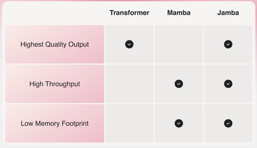
- The architecture of Jamba combines Transformer layers, Mamba layers, and mixture-of-experts (MoE) layers to optimize memory usage, computational throughput, and overall performance. One of the critical innovations is the use of MoE layers, allowing Jamba to selectively utilize just 12B out of its available 52B parameters during inference, making it significantly more efficient than a Transformer model of equivalent size.
- As depicted in the diagram below, AI21’s Jamba architecture features a blocks-and-layers approach that allows Jamba to successfully integrate the two architectures. Each Jamba block contains either an attention or a Mamba layer, followed by a multi-layer perceptron (MLP), producing an overall ratio of one Transformer layer out of every eight total layers.
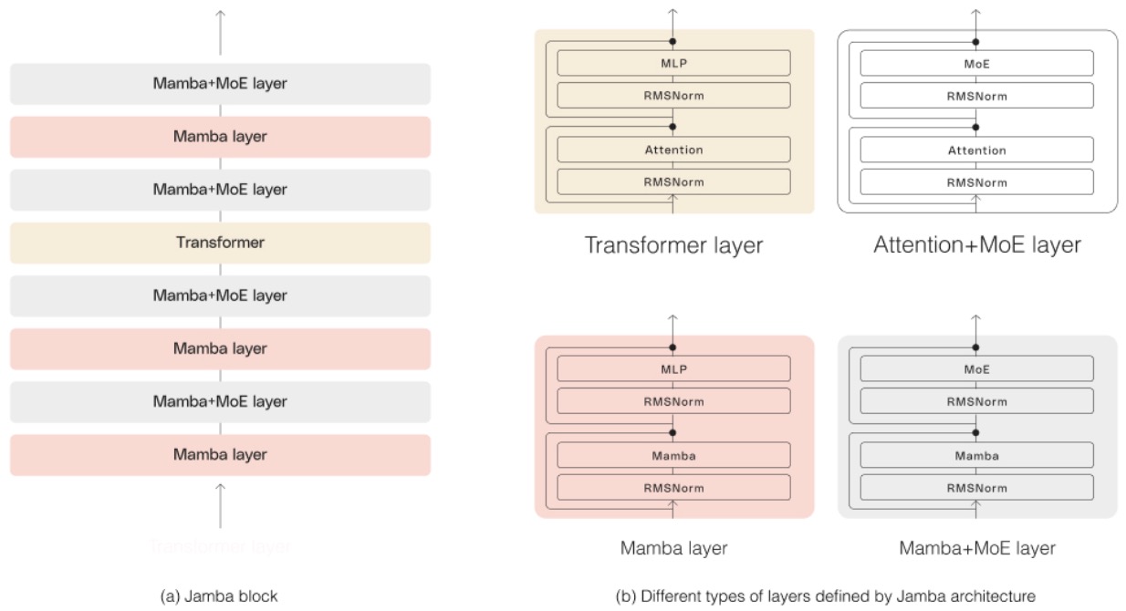
- Jamba has been scaled to a production-grade level, a feat previously unachieved by Mamba models beyond 3B parameters. Its architecture employs a blocks-and-layers design that alternates between attention or Mamba layers and multi-layer perceptrons (MLP), with a Transformer layer included for every eight total layers. This design is instrumental in optimizing the model for high-quality output and throughput on common hardware, such as a single 80GB GPU.
- Significant results have been observed in Jamba’s performance, with a 3x improvement in throughput on long contexts compared to similar models like Mixtral 8x7B, without compromising on efficiency. These achievements have been made possible by innovative engineering choices, including the strategic use of MoE layers to manage computational demands and the integration of Mamba with Transformer architectures for superior model capacity and efficiency.
- Jamba is released with open weights under Apache 2.0, encouraging further exploration and development within the AI community. Additionally, it’s made accessible via Hugging Face and is slated for inclusion in the NVIDIA API catalog, facilitating its adoption in enterprise applications through the NVIDIA AI Enterprise software platform.
Related Papers
Efficiently Modeling Long Sequences with Structured State Spaces
- The paper, authored by Gu et al. from Stanford University, introduces a new sequence model named Structured State Space Sequence model (S4), designed to efficiently handle long-range dependencies (LRDs) in data sequences extending over 10,000 steps or more.
- S4 leverages a novel parameterization of the state space model (SSM), enabling it to efficiently compute tasks while maintaining high performance traditionally achieved by models like RNNs, CNNs, and Transformers. Specifically, it uses a reparameterization of the structured state matrices in SSMs by combining a low-rank correction with a normal term, allowing for efficient computations via the Cauchy kernel, reducing the operational complexity to \(O(N+L)\) for state size \(N\) and sequence length \(L\).
- The model significantly outperforms existing models on the Long Range Arena benchmark, addressing tasks previously infeasible due to computational constraints. For example, it achieves 91% accuracy on sequential CIFAR-10 and solves the challenging Path-X task (16k length) with 88% accuracy, a task where other models performed no better than random.
- The figure below from the paper shows: (Left) State Space Models (SSM) parameterized by matrices \(A\), \(B\), \(C\), \(D\) map an input signal \(u(t)\) to output \(y(t)\) through a latent state \(x(t)\). (Center) Recent theory on continuous-time memorization derives special A matrices that allow SSMs to capture LRDs mathematically and empirically. (Right) SSMs can be computed either as a recurrence (left) or convolution (right). However, materializing these conceptual views requires utilizing different representations of its parameters (red, blue, green) which are very expensive to compute. S4 introduces a novel parameterization that efficiently swaps between these representations, allowing it to handle a wide range of tasks, be efficient at both training and inference, and excel at long sequences.
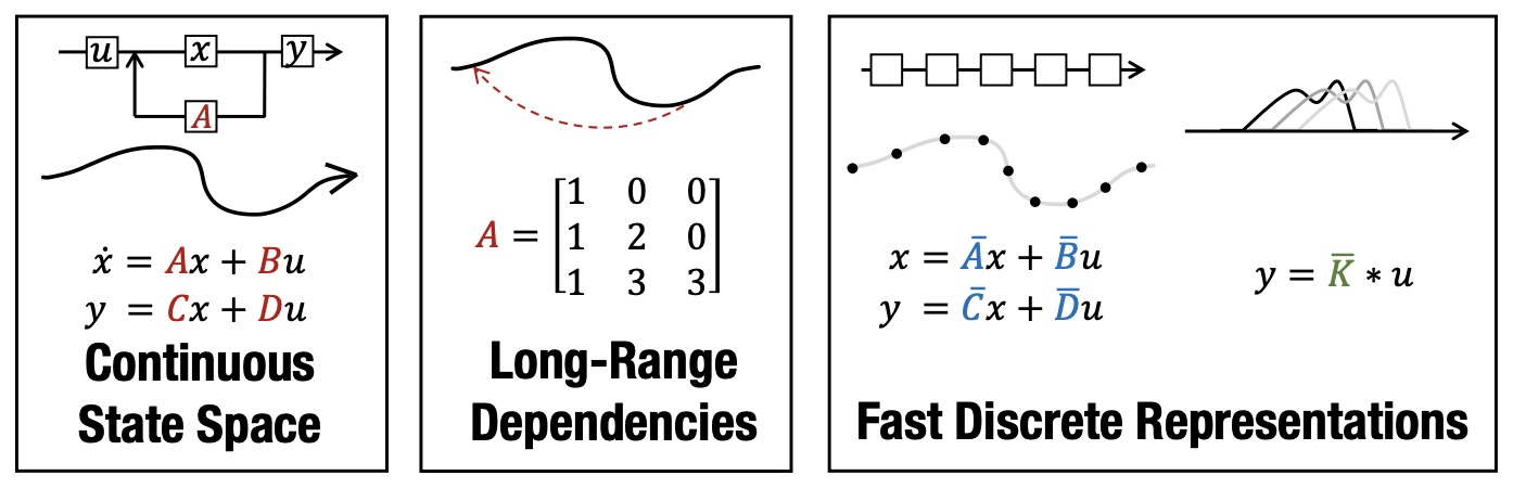
- Implementation details include the use of the HiPPO framework to derive specific matrices that help capture long-range dependencies more effectively. S4 transitions between continuous-time, recurrent, and convolutional representations of the SSM, which accommodates various data modalities and sequence lengths efficiently.
- Additionally, the paper discusses the architecture of the S4 layer in depth, detailing how it uses the state space to model sequences across different domains, such as images, audio, and text, with minimal domain-specific tailoring. It also explains how S4 handles changes in time-series sampling frequency without retraining, an important feature for real-world applications.
Mamba: Linear-Time Sequence Modeling with Selective State Spaces
- This paper by Gu and Dao from presents ‘Mamba’, a neural network architecture for sequence modeling. Mamba addresses the computational inefficiencies of Transformers in processing long sequences, a significant issue in modern deep learning, particularly with foundation models.
- They propose selective state space models (SSMs) that enable linear scaling with sequence length and demonstrate superior performance across different modalities including language, audio, and genomics.
- The authors highlight that traditional SSMs struggle with discrete and information-dense data like text due to their inability for content-based reasoning. By making SSM parameters input-dependent, Mamba can selectively process information, improving its adaptability and performance. This innovative approach allows selective information retention across sequences, crucial for coherent text generation and understanding.
- To maintain computational efficiency despite the loss of efficient convolution operations due to input-dependent parameters, the authors develop a hardware-aware parallel algorithm for SSM computation. This innovation avoids extensive memory access and leverages GPU memory hierarchy effectively, leading to significant speedups. The architecture integrates these selective SSMs into a single block, eliminating the need for attention or MLP blocks, resulting in a homogeneous and efficient design.
- Mamba’s architecture simplifies previous deep sequence models by integrating selective SSMs without the need for attention or MLP blocks, achieving a homogeneous and simplified design. This results in a model that not only performs well on tasks requiring long-range dependencies but also offers rapid inference. The following figure from the paper shows: (Overview.) Structured SSMs independently map each channel (e.g., \(D\) = 5) of an input \(x\) to output \(y\) through a higher dimensional latent state \(h\) (e.g., \(N\) = 4). Prior SSMs avoid materializing this large effective state (\(DN\), times batch size \(B\) and sequence length \(L\)) through clever alternate computation paths requiring time-invariance: the \((\Delta, A, B, C)\) parameters are constant across time. Mamba’s selection mechanism adds back input-dependent dynamics, which also requires a careful hardware-aware algorithm to only materialize the expanded states in more efficient levels of the GPU memory hierarchy.
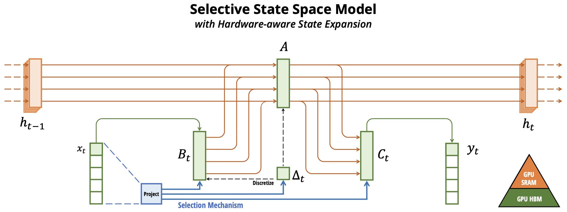
- In empirical evaluations, Mamba sets new performance benchmarks in tasks such as selective copying and induction heads, showcasing its ability to solve problems that challenge other models. In language modeling, Mamba outperforms Transformers of similar or even larger sizes, offering better scaling laws and downstream task performance. Additionally, in DNA modeling and audio generation, Mamba achieves state-of-the-art results, benefiting from its ability to process long sequences efficiently.
- Mamba demonstrates superior performance in various tasks like language, audio, and genomics. It outperforms Transformers of the same size in language modeling and achieves five times higher throughput, scaling linearly in sequence length. Its versatility is showcased through empirical validation on tasks such as synthetic copying, induction heads, language modeling, DNA modeling, and audio modeling and generation. The model’s significant speed improvements and scalability could redefine efficiency standards in foundation models across different modalities.
- The paper also discusses the significance of the selection mechanism in SSMs, connecting it to gating mechanisms in recurrent neural networks and highlighting its role in modeling variable spacing and context in sequences. This mechanism allows Mamba to focus on relevant information and ignore noise, which is crucial for handling long sequences in various domains.
- Model ablations and comparisons demonstrate the critical components contributing to Mamba’s performance, including the impact of selective parameters and the architecture’s simplified design. The authors release the model code and pre-trained checkpoints, facilitating further research and application in the field.
MambaByte: Token-free Selective State Space Model
- This paper by Wang et al. from Cornell introduced MambaByte, a novel adaptation of the Mamba state space model designed for efficient language modeling directly from raw byte sequences. Addressing the challenges posed by the significantly longer sequences of bytes compared to traditional subword units, MambaByte leverages the computational efficiency of state space models (SSMs) to outperform existing byte-level models and rival state-of-the-art subword Transformers.
- MambaByte’s architecture is distinguished by its selective mechanism tailored for discrete data like text, enabling linear scaling in length and promising faster inference speeds compared to conventional Transformers. This breakthrough is attributed to the model’s ability to efficiently process the extended sequences inherent to byte-level processing, eliminating the need for subword tokenization and its associated biases.
- The figure below from the paper shows a Mamba block. \(\sigma\) indicates Swish activation.
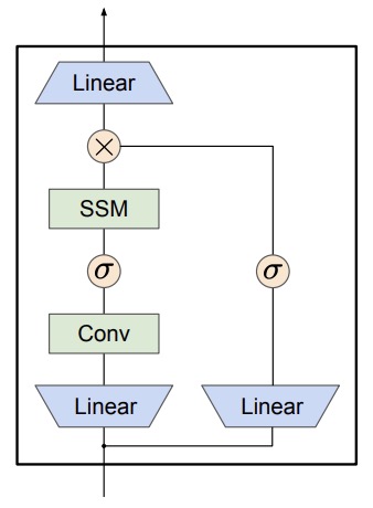
- Experimental results highlight MambaByte’s superior performance and computational efficiency. Benchmarks on the PG19 dataset and comparisons with other byte-level models, including the MegaByte Transformer and gated diagonalized S4, demonstrated MambaByte’s reduced computational demands and enhanced effectiveness in language modeling tasks. Its capability to maintain competitive performance with significantly longer sequences without relying on tokenization marks a substantial advancement in language model training.
- The figure below from the paper shows the benchmarking byte-level models with a fixed parameter budget. Language modeling results on PG19 (8, 192 consecutive bytes), comparing the standard Transformer, MegaByte Transformer, gated diagonalized S4, and MambaByte. (Left) Model loss over training step. (Right) FLOP-normalized training cost. MambaByte reaches Transformer loss in less than one-third of the compute budget.
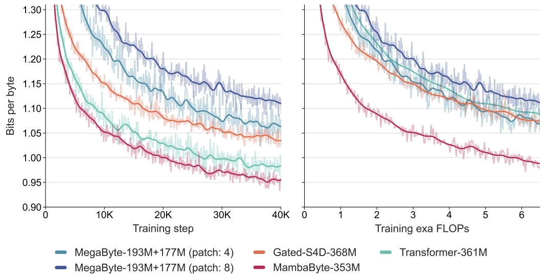
- The paper provides a comprehensive analysis of the MambaByte model, including its experimental setup, dataset specifics, and detailed implementation techniques. The study meticulously outlines the comparative evaluation of MambaByte against other models under fixed parameter and compute settings across several long-form text datasets. Furthermore, it delves into the selective state space sequence modeling background that underpins MambaByte’s design, offering insights into the model’s operational efficiency and practicality for large-scale language processing tasks.
- MambaByte’s introduction as a token-free model that effectively addresses the inefficiencies of byte-level processing while rivaling the performance of subword models is a significant contribution to the field of natural language processing. Its development paves the way for future explorations into token-free language modeling, potentially influencing large-scale model training methodologies and applications.
- Code
Scalable Diffusion Models with State Space Backbone
- This paper by Fei et al. from Kunlun Inc. introduces a novel approach to scaling diffusion models using a state space architecture.
- They focus on replacing the traditional U-Net backbone with a state space model (SSM) framework to enhance image generation performance and computational efficiency.
- The authors present Diffusion State Space Models (DiS) that treat all inputs—time, condition, and noisy image patches—as discrete tokens, enhancing the model’s ability to handle long-range dependencies effectively. The DiS architecture is characterized by its scalability, leveraging state space techniques that offer superior performance compared to conventional CNN-based or Transformer-based architectures, especially in handling larger image resolutions and reducing computational costs.
- Key Technical Details and Implementation:
- Architecture: DiS utilizes a state space model backbone which processes inputs as tokens, incorporating forward and backward processing with skip connections that enhance both shallow and deep layers’ integration.
- Noise Prediction Network: The noise prediction network in DiS, represented as \(\epsilon_\theta(x_t, t, c)\), predicts the injected noise at various timesteps and conditions, thereby optimizing the reverse diffusion process from noisy to clean images.
- Model Configurations: Different configurations of DiS are explored, with parameters adjusted for varying depths and widths, showing a clear correlation between increased model complexity and improved image quality metrics.
- Patchify and Linear Decoder: Initial layers transform input images into a sequence of tokens which are then processed by SSM blocks. The output is decoded back to image space using a linear decoder after the final SSM block, predicting noise and covariance matrices.
- The following figure from the paper shows the proposed state space-based diffusion models. It treats all inputs including the time, condition and noisy image patches as tokens and employs skip connections between shallow and deep layers. Different from original Mamba for text sequence modeling, our SSM block process the hidden states sequence with both forward and backward directions.
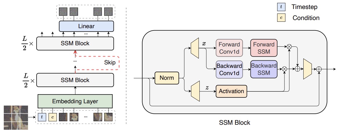
- DiS models were tested under unconditional and class-conditional image generation tasks. In scenarios like ImageNet at resolutions of 256 \(\times\) 256 and 512 \(\times\) 512 pixels, DiS models demonstrated competitive or superior performance to prior models, achieving impressive Frechet Inception Distance (FID) scores.
- Various configurations from small to huge models were benchmarked to demonstrate scalability, showing that larger models continue to provide substantial improvements in image quality.
- The paper concludes that DiS models not only perform comparably or better than existing architectures but do so with less computational overhead, showcasing their potential in scalable and efficient large-scale image generation. This approach paves the way for future explorations into more effective generative modeling techniques that can handle complex, high-resolution datasets across different modalities. The authors also make their code and models publicly available, encouraging further experimentation and development in the community.
Cobra: Extending Mamba to Multi-Modal Large Language Model for Efficient Inference
- This paper by Zhao et al. from Westlake University and Zhejiang University introduces Cobra, in response to the growing need for efficient multi-modal large language models (MLLMs). This model enhances the efficiency of MLLMs by incorporating a linear computational complexity approach through the use of the state space model (SSM) framework, distinct from the common quadratic complexity of traditional Transformer networks.
- Cobra extends the Mamba model by integrating visual information processing capabilities. This integration is achieved through a combination of an image encoder and a novel training methodology. The Mamba model, known for its efficient processing relative to Transformer-based models, is enhanced with visual modality by incorporating an image encoder that allows for the efficient handling of visual data.
- A significant feature of Cobra is its modal fusion approach, which optimizes the interaction between visual and linguistic data. Various fusion schemes were explored, with experiments showing that specific strategies significantly enhance the model’s multi-modal capabilities.
- The model demonstrates its effectiveness across multiple benchmarks, particularly in tasks like Visual Question Answering (VQA), where it competes robustly against other state-of-the-art models like LLaVA and TinyLLaVA, despite having fewer parameters. For instance, Cobra achieved performance comparable to LLaVA while utilizing only about 43% of LLaVA’s parameters.
- The architectural design of Cobra includes a combination of DINOv2 and SigLIP as vision encoders, projecting visual information into the language model’s embedding space. This setup not only preserves but enhances the model’s ability to process and understand complex visual inputs alongside textual data.
- Training adjustments and implementation details reveal a departure from traditional pre-alignment phases used in other models. Instead, Cobra’s approach involves direct fine-tuning of the entire LLM backbone along with the projector over two epochs, which optimizes both efficiency and model performance.
- The figure below from the paper shows a detailed architecture of Cobra (right) that takes Mamba as the backbone consisting of identical Mamba blocks (left). The parameters of vision encoders are frozen during training.
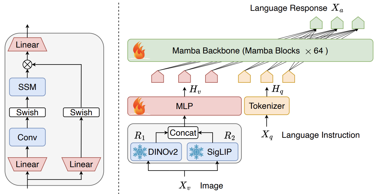
- Performance metrics from the paper indicate that Cobra is not only faster but also retains high accuracy in interpreting and responding to multi-modal inputs, showing particularly strong capabilities in handling visual illusions and spatial relationships, a testament to its robust visual processing capabilities.
- Overall, Cobra’s design significantly reduces the computational cost and model complexity while maintaining competitive accuracy and speed, making it a promising solution for applications requiring efficient and effective multi-modal processing.
- Code
SAMBA: Simple Hybrid State Space Models for Efficient Unlimited Context Language Modeling
- This paper introduces SAMBA, a novel hybrid architecture that combines Mamba, a selective State Space Model (SSM), with Sliding Window Attention (SWA) to efficiently model sequences with infinite context length. The authors address the challenge of balancing computation complexity and the ability to generalize to longer sequences than seen during training. SAMBA leverages the strengths of both SSMs and attention mechanisms to achieve linear-time complexity while maintaining precise memory recall.
- SAMBA architecture consists of three main components: Mamba layers, SWA layers, and Multi-Layer Perceptrons (MLPs). Mamba layers capture time-dependent semantics and compress sequences into recurrent hidden states. SWA layers, operating on a window size of 2048, provide precise retrieval of non-Markovian dependencies within the sequence. MLP layers handle nonlinear transformations and recall of factual knowledge, enhancing the model’s overall capability.
- The SAMBA model was scaled to 3.8B parameters and trained on 3.2T tokens. It demonstrated superior performance compared to state-of-the-art models based on pure attention or SSMs across various benchmarks, including commonsense reasoning, language understanding, truthfulness, and math and coding tasks. Notably, SAMBA showed improved token predictions up to 1M context length and achieved a 3.73× higher throughput than Transformers with grouped-query attention when processing 128K length user prompts.
- The figure below from the paper illustrates from left to right: Samba, Mamba-SWA-MLP, Mamba-MLP, and Mamba. The illustrations depict the layer-wise integration of Mamba with various configurations of Multi-Layer Perceptrons (MLPs) and Sliding Window Attention (SWA). They assume the total number of intermediate layers to be \(N\), and omit the embedding layers and output projections for simplicity. Pre-Norm and skip connections are applied for each of the intermediate layers.
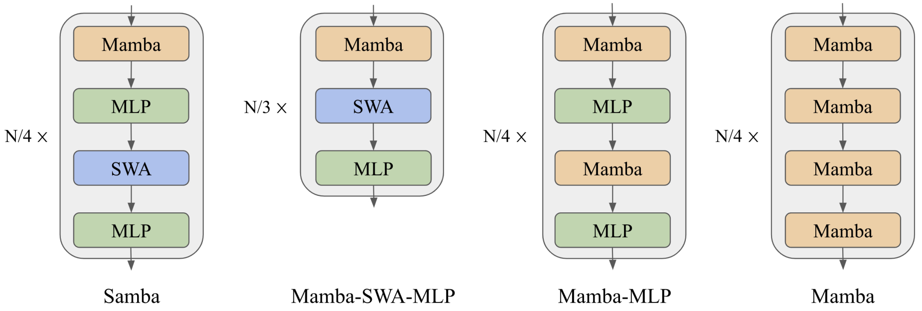
- The implementation of SAMBA involved meticulous exploration of hybridization strategies, including different layer-wise combinations of Mamba, SWA, and MLP. The final configuration was optimized for performance, with a total of 48 layers for Samba and Mamba-MLP models, and 54 layers for the Mamba-SWA-MLP model. The models were pre-trained on the Phi-2 dataset with 4K sequence lengths, and downstream evaluations were conducted on a range of benchmarks to validate the architectural design.
- SAMBA’s ability to extrapolate context length was tested extensively. It maintained linear decoding time complexity with unlimited token streaming, achieving perfect memory recall and improved perplexity on long sequences. The model’s performance on long-context summarization tasks further demonstrated its efficiency and effectiveness in handling extensive contexts.
- In conclusion, SAMBA presents a significant advancement in language modeling, offering a simple yet powerful solution for efficient modeling of sequences with unlimited context length. The hybrid architecture effectively combines the benefits of SSMs and attention mechanisms, making it a promising approach for real-world applications requiring extensive context understanding.
- Code
Further Reading
SSMs
RWKV
- Related resources to understand RWKV, another architecture that converts self-attention to a linear operation:
- Intro to RWKV presents an overview of the RWKV language model, an RNN that combines the benefits of transformers, offering efficient training, reduced memory use during inference, and excellent scaling up to 14 billion parameters, while being an open-source project open for community contribution.
- Annotated RWKV offers 100 lines of code to implement a basic version of RWKV.
References
State Space Model and HiPPO foundations
- HiPPO: Recurrent Memory with Optimal Polynomial Projections by Gu et al. (2020)
- Combining Recurrent, Convolutional, and Continuous-time Models with Linear State Space Layers by Gu et al. (2021)
- How to Train Your HiPPO: State Space Models with Generalized Orthogonal Basis Projections by Gu et al. (2022)
- Liquid Structural State-Space Models by Hasani et al. (2022)
S4 and structured State Space Models
- Efficiently Modeling Long Sequences with Structured State Spaces by Gu et al. (2022); The Annotated S4 by Rush and Karamcheti; The State Space Models Blog: S4 Part 1 by Hazy Research; S4 Part 2 by Hazy Research; S4 Part 3 by Hazy Research
- Diagonal State Spaces are as Effective as Structured State Spaces by Gupta et al. (2022)
- On the Parameterization and Initialization of Diagonal State Space Models by Gu et al. (2022)
- Simplified State Space Layers for Sequence Modeling by Smith et al. (2023); S5 implementation by Smith et al.
State Space Models for language modeling
- Hungry Hungry Hippos: Towards Language Modeling with State Space Models by Fu et al. (2023); Hungry Hungry Hippos: State Space Models for Language Modeling by Hazy Research; H3 implementation by Hazy Research
- Hyena Hierarchy: Towards Larger Convolutional Language Models by Poli et al. (2023)
- RWKV: Reinventing RNNs for the Transformer Era by Peng et al. (2023)
- Retentive Network: A Successor to Transformer for Large Language Models by Sun et al. (2023)
- GateLoop: Fully Data-Controlled Linear Recurrence for Sequence Modeling by Katsch (2023)
- Gated Linear Attention Transformers with Hardware-Efficient Training by Yang et al. (2024)
Mamba and selective State Space Models
- Mamba: Linear-Time Sequence Modeling with Selective State Spaces by Gu and Dao (2023); Official Mamba implementation by State Spaces
- MambaByte: Token-free Selective State Space Model by Wang et al. (2024); MambaByte implementation by Wang et al.
- MoE-Mamba: Efficient Selective State Space Models with Mixture of Experts by Pióro et al. (2024)
- A Visual Guide to Mamba and State Space Models by Grootendorst
Structured State Space Duality and Mamba-2
- Transformers are SSMs: Generalized Models and Efficient Algorithms Through Structured State Space Duality by Dao and Gu (2024); ICML publication by Dao and Gu; Official Mamba and Mamba-2 implementation by State Spaces
Mamba-3 and inference-oriented SSMs
- Mamba-3: Improved Sequence Modeling using State Space Principles by Lahoti et al. (2026); Official Mamba-3 implementation by State Spaces
Hybrid Mamba-attention architectures
- Jamba: A Hybrid Transformer-Mamba Language Model by Lieber et al. (2024)
- Zamba: A Compact 7B SSM Hybrid Model by Glorioso et al. (2024)
- Griffin: Mixing Gated Linear Recurrences with Local Attention for Efficient Language Models by De et al. (2024)
- Taipan: Efficient and Expressive State Space Language Models with Selective Attention by Yang et al. (2024)
- Nemotron-H: A Family of Accurate and Efficient Hybrid Mamba-Transformer Models by NVIDIA et al. (2025)
Recall, associative memory, and recurrent-state capacity
- Zoology: Measuring and Improving Recall in Efficient Language Models by Arora et al. (2024)
- Simple Linear Attention Language Models Balance the Recall-Throughput Tradeoff by Arora et al. (2024); ICML publication; Based: Simple Linear Attention Language Models Balance the Recall-Throughput Tradeoff by Hazy Research; Based implementation by Hazy Research
Linear attention and recurrent alternatives
- Retentive Network: A Successor to Transformer for Large Language Models by Sun et al. (2023)
- Gated Linear Attention Transformers with Hardware-Efficient Training by Yang et al. (2024); ICML publication
- GateLoop: Fully Data-Controlled Linear Recurrence for Sequence Modeling by Katsch (2023)
- RWKV: Reinventing RNNs for the Transformer Era by Peng et al. (2023)
- Hyena Hierarchy: Towards Larger Convolutional Language Models by Poli et al. (2023)
Attention systems and IO-aware sequence processing
- FlashAttention: Fast and Memory-Efficient Exact Attention with IO-Awareness by Dao et al. (2022); FlashAttention implementation by Dao et al.
- FlashAttention-2: Faster Attention with Better Parallelism and Work Partitioning by Dao (2023); FlashAttention-2 implementation by Dao
- Simple Linear Attention Language Models Balance the Recall-Throughput Tradeoff by Arora et al. (2024): develops IO-aware linear-attention kernels and frames recurrent-state size, recall, and generation throughput as a joint systems tradeoff.
- Gated Linear Attention Transformers with Hardware-Efficient Training by Yang et al. (2024): develops FlashLinearAttention and hardware-efficient chunkwise algorithms for gated linear attention.
Vision State Space Models
- Vision Mamba: Efficient Visual Representation Learning with Bidirectional State Space Model by Zhu et al. (2024); ICML publication
- VMamba: Visual State Space Model by Liu et al. (2024)
- State Space Models for Event Cameras by Zubić et al. (2024)
Video State Space Models
- VideoMamba: State Space Model for Efficient Video Understanding by Li et al. (2024); VideoMamba implementation by Li et al.
Genomics and biological sequence modeling
- HyenaDNA: Long-Range Genomic Sequence Modeling at Single Nucleotide Resolution by Nguyen et al. (2023)
- Caduceus: Bi-Directional Equivariant Long-Range DNA Sequence Modeling by Schiff et al. (2024)
Reinforcement learning, control, and sequential decision making
- Decision S4: Efficient Sequence-Based RL via State Spaces Layers by Bar-David et al. (2023)
Core implementation and explanatory resources
- Mamba official repository by State Spaces: reference implementations and kernels for Mamba, Mamba-2, and Mamba-3
- S5 official repository by Smith et al.: JAX implementation of S5 and its parallel-scan formulation
- H3 official repository by Hazy Research: implementation of H3 and its SSM-based language-modeling architecture
- Based official repository by Hazy Research: implementation of Based and its IO-aware linear-attention kernels
- FlashAttention official repository by Dao et al.: optimized CUDA implementations of FlashAttention and FlashAttention-2
- The Annotated S4 by Rush and Karamcheti: implementation-oriented walkthrough of S4, discretization, convolutional execution, and structured kernels
- A Visual Guide to Mamba and State Space Models by Grootendorst: visual treatment of classical SSMs, HiPPO, S4, selective state spaces, and Mamba
Citation
If you found our work useful, please cite it as:
@article{Chadha2020DistilledStateSpaceModels,
  title   = {State Space Models},
  author  = {Chadha, Aman and Jain, Vinija},
  journal = {Distilled AI},
  year    = {2020},
  note    = {\url{https://vinija.ai}}
}