Primers • Separable Convolutions
- Separable Convolutions
- Spatially Separable Convolutions
- Depthwise Separable Convolutions
- References
- Citation
Separable Convolutions
- Anyone who takes a look at the architecture of MobileNet will undoubtedly come across the concept of separable convolutions. But what is that, and how is it different from a normal convolution?
- There are two main types of separable convolutions: spatially separable convolutions, and depthwise separable convolutions.
Spatially Separable Convolutions
- Conceptually, this is the easier one out of the two, and illustrates the idea of separating one convolution into two so let’s start with this. Unfortunately, spatially separable convolutions have some significant limitations, which hinders their widespread adoption in deep learning.
- Spatially separable convolutions are so named because it primarily deals with the spatial dimensions of an image and kernel: the width and the height. (The other dimension, the “depth” dimension, is the number of channels of each image).
- A spatially separable convolution simply factors a kernel into two smaller kernels. The most common case would be to divide a \(3 \times 3\) kernel into a \(3 \times 1\) and \(1 \times 3\) kernel, like so:
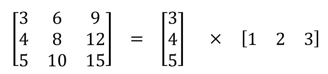
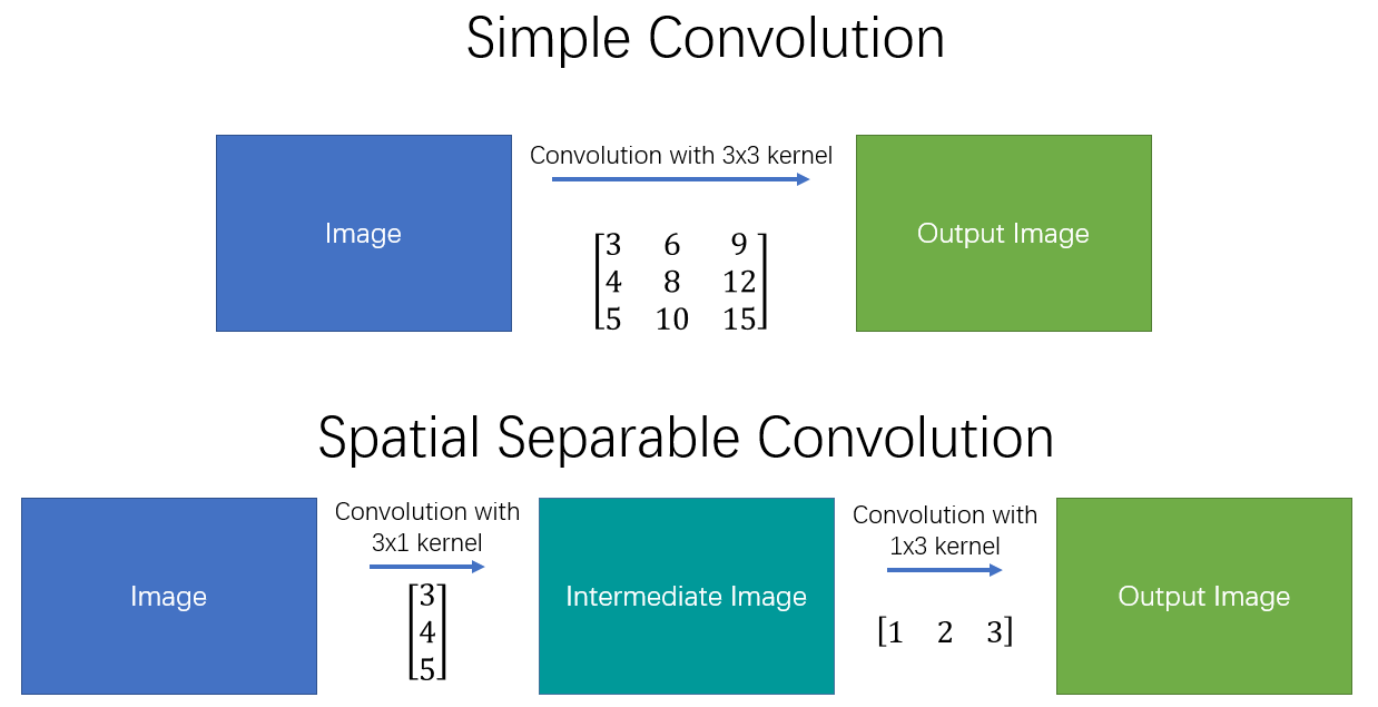
- Now, instead of doing one convolution with 9 multiplications, we do two convolutions with 3 multiplications each (6 in total) to achieve the same effect. With less multiplications, computational complexity goes down, and the network is able to run faster. The following diagram shows a simple and spatially separable convolution.
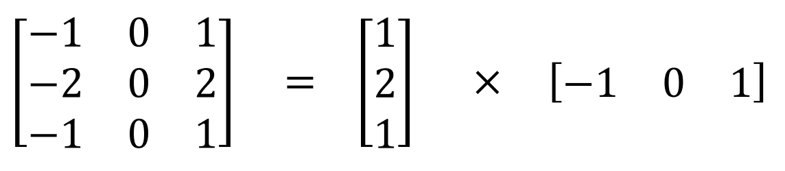
- One of the most famous convolutions that can be separated spatially is the Sobel kernel, used to detect edges:
- The main issue with the spatially separable convolution is that not all kernels can be “separated” into two, smaller kernels. This becomes particularly bothersome during training, since of all the possible kernels the network could have adopted, it can only end up using one of the tiny portion that can be separated into two smaller kernels.
Depthwise Separable Convolutions
- Unlike spatially separable convolutions, depthwise separable convolutions work with kernels that cannot be “factored” into two smaller kernels. Hence, it is more commonly used, especially in deep learning. This is the type of separable convolution seen in
keras.layers.SeparableConv2Dortf.layers.separable_conv2d. - The depthwise separable convolution is so named because it deals not just with the spatial dimensions, but with the depth dimension — the number of channels — as well. An input image may have 3 channels: RGB. After a few convolutions, an image may have multiple channels. You can image each channel as a particular interpretation of that image; in for example, the “red” channel interprets the “redness” of each pixel, the “blue” channel interprets the “blueness” of each pixel, and the “green” channel interprets the “greenness” of each pixel. An image with 64 channels has 64 different interpretations of that image. Similar to the spatially separable convolution, a depthwise separable convolution splits a kernel into two separate kernels that do two convolutions: the depthwise convolution and the pointwise convolution. But first of all, let’s see how a normal convolution works.
Normal Convolution
- If you don’t know how a convolution works from a 2-D perspective, read this article or check out this site.
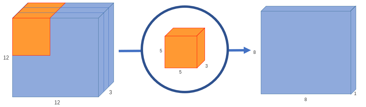
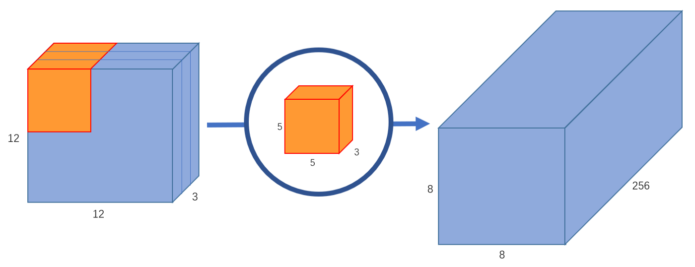
- A typical image, however, is not 2-D; it also has depth as well as width and height. Let us assume that we have an input image of \(12 \times 12 \times 3\) pixels, an RGB image of size \(12 \times 12\). Let’s do a \(5 \times 5\) convolution on the image with no padding and a stride of 1. If we only consider the width and height of the image, the convolution process is kind of like this: \((12 \times 12)\) \(\rightarrow\) (\(5 \times 5\)) \(\rightarrow\) \((8 \times 8)\). The \(5 \times 5\) kernel undergoes scalar multiplication with every 25 pixels, giving out1 number every time. We end up with a \(8 \times 8\) pixel image, since there is no padding (\(12–5+1 = 8\)).
- However, because the image has 3 channels, our convolutional kernel needs to have 3 channels as well. This means, instead of doing \(5 \times 5 = 25\) multiplications, we actually do \(5 \times 5 \times 3 = 75\) multiplications every time the kernel moves.
- Just like the 2-D interpretation, we do scalar matrix multiplication on every 25 pixels, outputting 1 number. After going through a \(5 \times 5 \times 3\) kernel, the \(12 \times 12 \times 3\) image will become a \(8 \times 8 \times 1\) image.
- What if we want to increase the number of channels in our output image? What if we want an output of size \(8 \times 8 \times 256\)?
- Well, we can create 256 kernels to create 256 \(8 \times 8 \times 1\) images, then stack them up together to create a \(8 \times 8 \times 256\) image output.
-
This is how a normal convolution works. Think of it like a function:
\[(12 \times 12 \times 3) \rightarrow (5 \times 5 \times 3 \times 256) \rightarrow (12 \times 12 \times 256)\]- where \(5 \times 5 \times 3 \times 256\) represents the height, width, number of input channels, and number of output channels of the kernel.
- Note that this is not matrix multiplication; we’re not multiplying the whole image by the kernel, but moving the kernel through every part of the image and multiplying small parts of it separately.
-
A depthwise separable convolution separates this process into two parts: a depthwise convolution and a pointwise convolution.
Part 1 — Depthwise Convolution
- In the first part, depthwise convolution, we give the input image a convolution without changing the depth. We do so by using 3 kernels of shape 5x5x1.
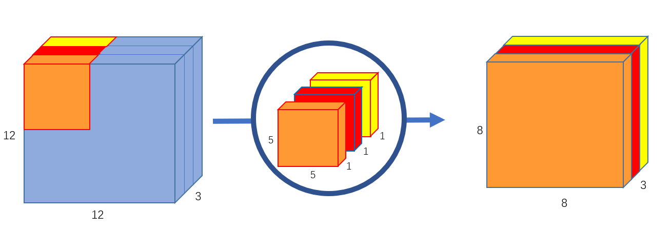
- Each 5x5x1 kernel iterates 1 channel of the image (note: 1 channel, not all channels), getting the scalar products of every 25 pixel group, giving out a 8x8x1 image. Stacking these images together creates a 8x8x3 image.
Part 2 — Pointwise Convolution
- Remember, the original convolution transformed a \(12 \times 12 \times 3\) image to a \(8 \times 8 \times 256\) image. Currently, the depthwise convolution has transformed the \(12 \times 12 \times 3\) image to a \(8 \times 8 \times 3\) image. Now, we need to increase the number of channels of each image.
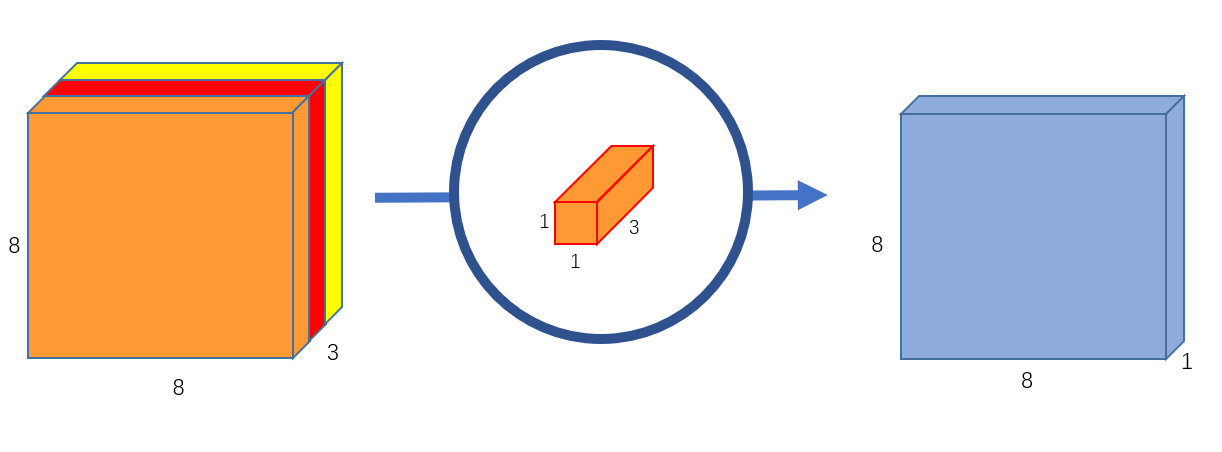
- The pointwise convolution is so named because it uses a \(1 \times 1\) kernel, or a kernel that iterates through every single point. This kernel has a depth of however many channels the input image has; in our case, 3. Therefore, we iterate a \(1 \times 1 \times 3\) kernel through our \(8 \times 8 \times 3\) image, to get a \(8 \times 8 \times 1\) image.
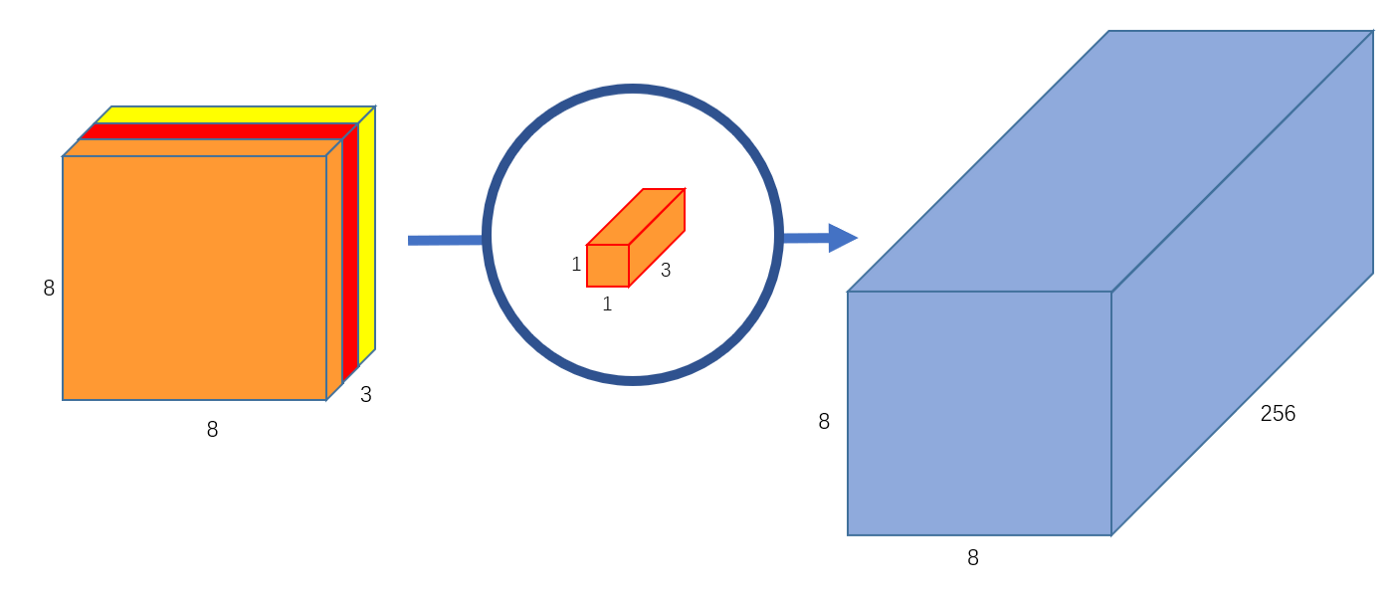
- We can create 256 \(1 \times 1 \times 3\) kernels that output a \(8 \times 8 \times 1\) image each to get a final image of shape \(8 \times 8 \times 256\).
-
And that’s it! We’ve separated the convolution into two: a depthwise convolution and a pointwise convolution. In a more abstract way, if the original convolution function is …
\[(12 \times 12 \times 3) \rightarrow (5 \times 5 \times 3 \times 256) \rightarrow (12 \times 12 \times 256)\]- … we can illustrate this new convolution as:
References
Citation
If you found our work useful, please cite it as:
@article{Chadha2020DistilledSeparableConvolutions,
  title   = {Separable Convolutions},
  author  = {Chadha, Aman},
  journal = {Distilled AI},
  year    = {2020},
  note    = {\url{https://aman.ai}}
}