Primers • Reinforcement Learning
- Overview
- Basics of Reinforcement Learning
- Offline vs. Online Reinforcement Learning
- Case Study: Online RL in Production Coding Agents
- Reward Design
- On-Policy Loops
- Instrumentation
- Evaluation
- Synthesis
- Types of Reinforcement Learning
- Value-Based Methods
- Policy-Based Methods
- Actor–Critic Methods
- Model-Based Reinforcement Learning
- Model-Free Reinforcement Learning
- On-Policy vs. Off-Policy Reinforcement Learning
- Deep Reinforcement Learning
- Deep Value-Based Methods
- Deep Policy-Based Methods
- Deep Actor–Critic Methods
- Deep Model-Based Methods
- Hybrid and Meta Deep Reinforcement Learning Methods
- Practical Considerations
- Tools and Frameworks for Deep Reinforcement Learning
- Policy Optimization for LLMs
- Model Roles
- Refresher: Notation Mapping between Classical RL and Language Modeling
- Policy Model
- Reference Model
- Reward Model
- Value Model
- Optimizing the Policy
- Integration of Policy, Reference, Reward, and Value Models in RLHF
- Model Roles
- Policy Evaluation
- Challenges of Reinforcement Learning
- Exploration vs. Exploitation Dilemma
- Sample Inefficiency
- Sparse and Delayed Rewards
- High-Dimensional State and Action Spaces
- Long-Term Dependencies and Credit Assignment
- Stability and Convergence
- Safety and Ethical Concerns
- Generalization and Transfer Learning
- Computational Resources and Scalability
- Reward Function Design
- FAQs
- References
- Citation
Overview
-
Reinforcement Learning (RL) is a type of machine learning where an agent learns to make sequential decisions by interacting with an environment. The goal of the agent is to maximize cumulative rewards over time by learning which actions yield the best outcomes in different states of the environment. Unlike supervised learning, where models are trained on labeled data, RL focuses on exploration and exploitation: the agent must explore various actions to discover high-reward strategies while exploiting what it has learned to achieve long-term success.
-
In RL, the agent, environment, actions, states, and rewards are fundamental components. At each step, the agent observes the state of the environment, chooses an action based on its policy (its strategy for selecting actions), and receives a reward that guides future decision-making. The agent’s objective is to learn a policy that maximizes the expected cumulative reward, typically by using techniques such as dynamic programming, Monte Carlo methods, or temporal-difference learning.
-
Deep RL extends traditional RL by leveraging deep neural networks to handle complex environments with high-dimensional state spaces. This allows agents to learn directly from raw, unstructured data, such as pixels in video games or sensors in robotic control. Deep RL algorithms, like Deep Q-Networks (DQN) and policy gradient methods (e.g., Proximal Policy Optimization, Group Relative Policy Optimization (GRPO), etc.), have achieved breakthroughs in domains like playing video games at superhuman levels, robotics, and autonomous driving.
-
This primer provides an introduction to the foundational concepts of RL, explores key algorithms, and outlines how deep learning techniques enhance the power of RL to tackle real-world, high-dimensional problems.
Basics of Reinforcement Learning
-
RL is a type of machine learning where an agent learns to make decisions by interacting with an environment. Unlike supervised learning, where a model learns from a fixed dataset of labeled examples, RL focuses on learning from the consequences of actions rather than from predefined correct behavior. The interaction between the agent and the environment is guided by the concepts of states, actions, rewards, and policies, which form the foundation of RL. The agent seeks to maximize cumulative rewards by exploring different actions and learning which ones yield the best outcomes over time.
-
Deep RL extends this framework by incorporating neural networks to handle high-dimensional, complex problems that traditional RL methods struggle with. By using deep learning techniques, Deep RL can tackle challenges like visual input or other high-dimensional data, allowing it to solve problems that are intractable for classical RL approaches. This combination of RL and neural networks enables agents to perform well in more complex environments with minimal manual intervention.
Key Components of Reinforcement Learning
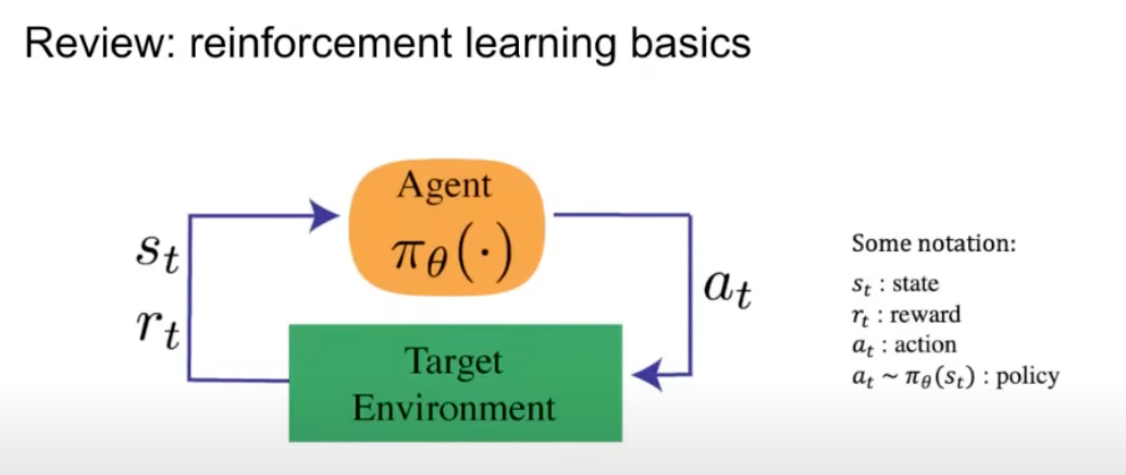
- At the core of RL is the interaction between an agent and an environment, as shown in the diagram below (source):
-
In this interaction, the agent takes actions in the environment and receives feedback in the form of states and rewards. The goal is for the agent to learn a strategy, or policy, that maximizes the cumulative reward over time.
-
Here are the critical components of RL:
-
Agent/Learner: The agent is the learner or decision-maker. It is responsible for selecting actions based on the current state of the environment.
-
Environment: Everything the agent interacts with. The environment defines the rules of the game, transitioning from one state to another based on the agent’s actions.
-
State (\(s\)): A representation of the environment at a particular point in time. States encapsulate all the information that the agent needs to know to make a decision. For example, in a video game, a state might be the current configuration of the game board.
-
Action (\(a\)): A decision taken by the agent in response to the current state. In each state, the agent must choose an action from a set of possible actions, which will affect the future state of the environment.
-
Reward (\(r\)): A scalar value that the agent receives from the environment after taking an action. The reward provides feedback on how good or bad an action was in that particular state. The agent’s objective is to maximize the cumulative reward over time, often referred to as the return.
-
Policy (\(\pi\)): A policy is the strategy the agent uses to determine the actions to take based on the current state. It is implemented as a mapping from states to action probabilities. It can be tabular, i.e., a simple lookup table mapping states to actions, or it can be more complex, such as a neural network in the case of deep RL. The policy can be deterministic (always taking the same action for a given state) or stochastic (taking different actions with some probability).
-
Value Function: The value function estimates how good (i.e., how much total expected reward) it is to be in a particular state (in which case, it is called the state-value function) or to take a specific action in that state (in which case, it is called the action-value function). It does so by accounting for both the immediate reward and the expected future rewards from subsequent states, helping the agent understand long-term reward potential rather than focusing only on immediate rewards. While value functions are of two types (i.e., state-value function and action-value function), the state-value function is also commonly called the value function. The relationship between the two is given by: \(V^{\pi}(s) = \sum_a \pi(a \mid s) Q^{\pi}(s, a)\), which means the value of a state under policy \(\pi\) is the expected action-value, averaged over all possible actions the policy might take in that state.
-
State-Value Function (V-function): Denoted as \(V^{\pi}(s)\), the state-value function measures the expected return (total discounted reward) starting from state \(s\) and then following policy \(\pi\) thereafter. It is formally defined as \(V^{\pi}(s) = \mathbb{E}_{\pi}\left[\sum_{t=0}^{\infty} \gamma^t r_t \mid s_0 = s\right]\), where \(\pi\) is the policy, \(\gamma \in [0,1)\) is the discount factor weighting future rewards, \(r_t\) is the reward received at time step \(t\), and the expectation \(\mathbb{E}_{\pi}[\cdot]\) is taken over trajectories generated by following policy \(\pi\).
-
Action-Value Function (Q-function): Denoted as \(Q(s, a)\) (where \(Q\) stands for “quality”), the action-value function measures the expected return for taking action \(a\) in state \(s\) and then following the policy \(\pi\) thereafter. It plays a central role in algorithms like Q-learning and Deep Q-Networks (DQN). It is formally defined as \(Q^{\pi}(s, a) = \mathbb{E}_{\pi}\left[\sum_{t=0}^{\infty} \gamma^t r_t \mid s_0 = s, a_0 = a\right]\), where the terms have the same meanings as above, except that the expectation begins from both a given state \(s\) and an initial action \(a\).
-
Advantage Function (\(A\)): The advantage function quantifies how much better taking a specific action \(a\) in state \(s\) is compared to the average action according to the policy. Put simply, the advantage function measures how much better the actual return was from a particular state than what was expected from that state before acting. It is is commonly used in policy gradient methods such as Actor-Critic and Proximal Policy Optimization (PPO) to reduce variance in gradient estimates. It is defined as \(\hat{A}(s, a) = Q(s, a) - V(s)\), where \(Q(s, a)\) is the action-value function (the expected return for taking action \(a\) in state \(s\) and then following the policy), and \(V(s)\) is the state-value function (the expected return from state \(s\) when following the policy).
-
Return (\(G\)): The total accumulated reward from a given time step onward, often discounted to prioritize near-term rewards \(G_t = \sum_{k=0}^{\infty} \gamma^k r_{t+k+1}\), where \(G\) stands for “gain” and \(\gamma\) is the discount factor that determines how much future rewards are valued relative to immediate rewards.
-
Discount Factor (\(\gamma\)): A scalar between 0 and 1 that controls the importance of future rewards. Smaller values make the agent myopic (focusing on immediate rewards), while larger values encourage long-term planning. Typically set closer to 1 to focus on long-term rewards rather than immediate ones.
-
Exploration vs. Exploitation: The trade-off between exploring new actions to discover potentially better rewards and exploiting known actions that already yield high rewards. Balancing these two is crucial for effective learning.
-
Trajectory/Episode/Rollout: A sequence of states, actions, rewards, and next states from the beginning of an episode to its termination, representing one complete interaction of the agent with the environment.
-
Temporal-Difference (TD) Error: The difference between the predicted value of a state and the observed reward plus the estimated value of the next state. It is used to update value estimates dynamically in methods like TD-learning, where the TD error is given by \(\delta_t = r_t + \gamma V(s_{t+1}) - V(s_t)\), with \(r_t\) as the immediate reward, \(\gamma\) the discount factor, and \(V(s_t)\) and \(V(s_{t+1})\) being the predicted values of the current and next states respectively.
-
Replay Buffer (Experience Replay): In Deep RL, a replay buffer stores past transitions (state, action, reward, next state) for sampling during training. This helps break correlation between consecutive samples—since experiences are drawn randomly rather than sequentially—allowing the agent to learn from a more diverse and independent set of experiences, which improves data efficiency and stabilizes training.
-
Actor-Critic Architecture: A hybrid approach combining a policy-based (actor) component that selects actions and a value-based (critic) component that evaluates them. The critic’s feedback stabilizes the actor’s learning.
-
The Bellman Equation
-
The Bellman Equation is a fundamental concept in RL, used to describe the relationship between the value of a state and the value of its successor states. It breaks down the value function into immediate rewards and the expected value of future states.
-
For a given policy \(\pi\), the state-value function \(V^{\pi}(s)\) can be written as:
\[V^{\pi}(s) = \mathbb{E}_\pi \left[ r_t + \gamma V^{\pi}(s_{t+1}) \mid s_t = s \right]\]- where:
- \(V^{\pi}(s)\) is the value of state \(s\) under policy \(\pi\),
- \(r_t\) is the reward received after taking an action at time \(t\),
- \(\gamma\) is the discount factor (0 ≤ \(\gamma\) ≤ 1) that determines the importance of future rewards,
- \(s_{t+1}\) is the next state after taking an action from state \(s\).
- where:
-
This equation expresses that the value of a state \(s\) is the immediate reward \(r_t\) plus the discounted value of the next state \(V^{\pi}(s_{t+1})\). The Bellman equation is central to many RL algorithms, as it provides the basis for recursively solving the optimal value function.
The RL Process: Trial and Error Learning
- The agent interacts with the environment in a loop:
- At each time step, the agent observes the current state of the environment.
- Based on this state, it selects an action according to its policy.
- The environment transitions to a new state, and the agent receives a reward.
- The agent uses this feedback to update its policy, gradually improving its decision-making over time.
- This process of learning from trial and error allows the agent to explore different actions and outcomes, eventually finding the optimal policy that maximizes the long-term reward.
Mathematical Formulation: Markov Decision Process (MDP)
- RL problems are typically framed as Markov Decision Processes (MDP), which provide a mathematical framework for modeling decision-making where outcomes are partly random and partly under the control of the agent. An MDP is defined by:
- States (\(S\)): The set of all possible states in the environment.
- Actions (\(A\)): The set of all possible actions the agent can take.
- Transition function (\(P\)): The probability distribution \(P(s_{t+1} \mid s_t, a_t)\) describing transitions from one state to another given an action.
- Reward function (\(R\)): The immediate reward \(R(s_t, a_t, s_{t+1})\) received after transitioning between states.
- Discount factor (\(\gamma\)): A scalar \(\gamma \in [0,1]\) controlling the importance of future rewards; values close to \(0\) emphasize immediate rewards, while values close to \(1\) emphasize long-term rewards.
-
The agent’s goal is to learn a policy \(\pi(s)\) that maximizes the expected cumulative reward (i.e., expected return), often expressed as:
\[G_t = \sum_{k=0}^{\infty} \gamma^k r_{t+k+1}\]- where:
- \(G_t\) is the total return starting from time step \(t\),
- \(\gamma\) is the discount factor,
- \(r_{t+k+1}\) is the reward received at time \(t+k+1\).
- where:
Offline vs. Online Reinforcement Learning
Offline Reinforcement Learning
-
Definition: Offline RL, also known as batch RL, refers to a RL paradigm where the agent learns solely from a pre-collected dataset of experiences without any interaction with the environment during training.
- Key Characteristics:
- Static Dataset: The dataset typically consists of tuples (state, action, reward, next state) that are collected by a specific policy, which could be suboptimal or from a combination of multiple policies.
- No Real-Time Interaction: Unlike online RL, the agent does not have the ability to gather new data or explore unknown parts of the state space.
- Policy Evaluation and Improvement: The primary goal is to learn a policy that generalizes well to the environment when deployed, leveraging the provided static data.
- Advantages:
- Safety and Cost-Effectiveness: Offline RL eliminates the risks and costs associated with real-world interactions, making it particularly valuable in -itical applications like healthcare or autonomous vehicles.
- Utilization of Historical Data: It allows researchers to leverage existing datasets, such as logs from previously deployed systems, for policy improvement without further data collection efforts.
- Challenges:
- Distributional Shift: The learned policy may take actions that lead to parts of the state space not covered in the dataset, resulting in poor performance (extrapolation error).
- Dependence on Dataset Quality: The effectiveness of the learning process is highly sensitive to the diversity and representativeness of the dataset.
- Overfitting: The agent might overfit to the static dataset, leading to poor generalization in unseen scenarios.
- Techniques to Address Challenges:
- Conservative Algorithms: Methods like Conservative Q-Learning (CQL) restrict the agent from overestimating out-of-distribution actions.
- Uncertainty Estimation: Leveraging uncertainty-aware models to avoid relying on poorly represented regions of the dataset.
- Offline-Optimized Models: Algorithms such as Batch Constrained Q-Learning (BCQ) and Behavior Regularized Actor-Critic (BRAC) are designed specifically for offline settings.
- Use Cases:
- Healthcare: Training models on patient treatment records to recommend actions without real-time experimentation.
- Autonomous Driving: Leveraging driving logs to improve decision-making policies without the risks of on-road testing.
- Robotics: Using pre-recorded demonstration data to teach robots tasks without additional data collection.
Online Reinforcement Learning
-
Definition: Online RL involves continuous interaction between the agent and the environment during training. The agent collects data through trial and error, allowing it to refine its policy iteratively in real time.
- Key Characteristics:
- Active Data Collection: The agent explores the environment to gather new experiences, enabling adaptation to dynamic or previously unseen states.
- Feedback Loop: There is a direct link between the agent’s actions, the environment’s responses, and policy improvement.
- Exploration-Exploitation Tradeoff: Balancing the exploration of new actions and the exploitation of learned strategies is a critical aspect of online RL.
- Advantages:
- Dynamic Adaptation: The agent can dynamically adapt to changes in the environment, ensuring robust performance.
- Optimal Exploration: By actively engaging with the environment, the agent can learn optimal strategies even in highly complex state spaces.
- Challenges:
- Exploration Risks: Excessive exploration can lead to suboptimal or dangerous actions, particularly in high-stakes applications.
- Resource-Intensive: Online RL requires significant computational and environmental resources due to real-time interaction.
- Stability and Convergence: Ensuring stable learning and avoiding divergence are ongoing research challenges.
- Techniques to Address Challenges:
- Exploration Strategies: Methods like epsilon-greedy, softmax exploration, or intrinsic motivation frameworks guide effective exploration.
- Stability Enhancements: Algorithms like Proximal Policy Optimization (PPO) and Trust Region Policy Optimization (TRPO) improve convergence stability.
- Efficient Learning: Techniques like prioritized experience replay and model-based RL improve data efficiency.
- Use Cases:
- Robotics: Training robots in simulated environments with the ability to transfer learned policies to the real world.
- Games: Developing agents that play video games, such as AlphaGo or OpenAI Five, through millions of simulated interactions.
- Dynamic Systems: Adapting to real-world systems with changing conditions, such as stock trading or energy management.
Comparative Analysis
| Aspect | Offline RL | Online RL |
|---|---|---|
| Data Source | Fixed, pre-collected dataset | Real-time interaction |
| Exploration | Not possible; constrained by dataset | Required |
| Learning | Static learning from a fixed dataset | Dynamic and iterative |
| Environment Access | No interaction during training | Continuous interaction |
| Main Challenges | Distributional shift, dataset quality | Exploration-exploitation balance, stability |
| Efficiency | Efficient with quality datasets | Resource-intensive |
| Use Cases | Healthcare, autonomous driving, robotics | Games, robotics, dynamic systems |
Hybrid Approaches
- Hybrid RL approaches combine the strengths of both paradigms. A typical strategy involves:
- Offline Pretraining: Using offline RL to initialize the agent’s policy with a high-quality dataset.
- Online Fine-Tuning: Allowing the agent to interact with the environment to refine its policy and improve performance further.
- Advantages:
- Combines safety and efficiency of offline training with the adaptability of online learning.
- Accelerates convergence by leveraging prior knowledge from pretraining.
- Examples:
- Autonomous Driving: Pretraining on driving logs followed by fine-tuning in simulation or controlled environments.
- Healthcare: Learning from historical patient data and adapting through real-time interactions in clinical trials.
Case Study: Online RL in Production Coding Agents
- Online reinforcement learning is especially useful when the training environment can be made close to the deployment environment, because the policy can learn from feedback generated by the same distribution of states, actions, and users it will encounter at inference time. In coding agents, this matters because the “environment” includes not only files, terminals, tests, and tool calls, but also the developer’s intent, tolerance for interruption, willingness to accept a suggestion, and reaction to partially correct edits. This makes user feedback a central part of the reward signal in production systems such as Improving Cursor Tab with online RL and Improving Composer through real-time RL.
From static post-training to online learning
-
Traditional model post-training often relies on static datasets, simulated tasks, paid annotation, or benchmark-driven optimization. In contrast, online RL updates the policy using fresh trajectories sampled from the current or nearly current deployed policy. This distinction is important because the policy-gradient estimator is naturally on-policy: once the policy parameters change, trajectories collected by the old policy are no longer exactly distributed according to the policy being optimized. Policy Gradient Methods for Reinforcement Learning with Function Approximation by Sutton et al. (2000) formalizes this direct optimization view of a parameterized stochastic policy, while Simple Statistical Gradient-Following Algorithms for Connectionist Reinforcement Learning by Williams (1992) introduces REINFORCE-style likelihood-ratio updates for increasing the probability of actions that yield higher reward.
-
For a policy \(\pi_\theta(a \mid s)\), the online RL objective can be written as:
\[J(\theta) = \mathbb{E}_{s \sim d^{\pi_\theta}, a \sim \pi_\theta(\cdot \mid s)}[R(s,a)]\]-
where \(d^{\pi_\theta}\) is the state distribution induced by the current policy and \(R(s,a)\) is the reward derived from user or environment feedback. The policy-gradient theorem gives the estimator:
\[\nabla_\theta J(\theta) =\mathbb{E}_{s \sim d^{\pi_\theta}, a \sim \pi_\theta(\cdot \mid s)} \left[ \nabla_\theta \log \pi_\theta(a \mid s) R(s,a) \right]\]
-
-
This equation explains why production online RL systems must minimize the delay between serving a checkpoint, collecting interaction data, computing rewards, updating weights, evaluating regressions, and redeploying the next checkpoint. If the delay becomes too large, the training data becomes stale relative to the policy being optimized, increasing off-policy mismatch.
Cursor Tab as online policy optimization
-
Cursor Tab frames autocomplete as a policy that must decide both what to suggest and whether to suggest anything at all. This is a natural RL problem because an action can be useful, distracting, or unnecessary depending on the developer’s next move. Improving Cursor Tab with online RL describes a production loop in which Tab runs on every user action, observes acceptance or rejection feedback, and updates the model using online policy-gradient training rather than merely training a separate acceptance classifier.
-
A simplified reward design illustrates the control problem. Suppose a suggestion should be shown only when the probability of acceptance exceeds a threshold \(\tau = 0.25\). Define:
- If the model shows a suggestion with acceptance probability \(p\), the expected reward is:
- Thus, showing a suggestion has positive expected reward exactly when:
- This reward construction converts “knowing when not to interrupt” into a learned policy behavior. Rather than optimizing only next-token likelihood, the model is optimized for the product-level action boundary between helpful completion and distracting suggestion. In the reported system, the resulting Tab model produced fewer suggestions while improving the acceptance rate, indicating that the policy learned to suppress low-confidence or low-value actions rather than merely generating more completions.
Composer and real-time RL from production trajectories
-
Composer extends the same online-RL principle from autocomplete to agentic coding. In this setting, an action may include edits, tool calls, terminal commands, file reads, clarifying questions, and multi-step plans. Improving Composer through real-time RL describes a real-time RL loop that serves model checkpoints to production, observes user responses, aggregates those responses into reward signals, trains on large batches of real interaction tokens, runs regression evaluations, and deploys improved checkpoints behind Auto as often as every five hours.
-
The following figure (source) shows Composer’s real-time RL reward improving across training steps, illustrating the intended effect of repeatedly converting production interaction data into reward-weighted policy updates.

-
The key motivation is train-test mismatch. Simulated coding environments can reproduce files, commands, tests, and repository structure with relatively high fidelity, but they struggle to reproduce the human developer supervising the agent. Research on human and user simulation, such as Generative Agents: Interactive Simulacra of Human Behavior by Park et al. (2023) and Using Large Language Models to Simulate Multiple Humans and Replicate Human Subject Studies by Aher et al. (2023), shows that language models can approximate some human-like behaviors, but simulated users can still introduce modeling error.
-
Real-time RL reduces this mismatch by using real production interactions as the feedback source. The environment is no longer only a benchmark harness; it is the deployed editor, the developer’s repository, the user’s task, and the user’s subsequent behavior. This makes the learned reward closer to the product objective, but it also makes the training loop more operationally demanding: instrumentation must convert user interactions into reliable signals, data pipelines must aggregate those signals quickly, training must run on large batches, and deployment must be fast enough to keep the data nearly on-policy.
Reward design and reward hacking
-
Real-time RL increases the importance of reward design because the model can discover weaknesses anywhere in the production feedback loop. If broken tool calls are excluded from training, a model may learn that invalid tool use avoids negative feedback. If edit-derived rewards penalize bad edits but do not penalize excessive deferral, a model may learn to ask clarifying questions instead of attempting useful edits. These are examples of reward hacking, where the learned policy optimizes the measured objective rather than the intended objective. Concrete Problems in AI Safety by Amodei et al. (2016) identifies reward hacking as a practical safety problem that arises when the specified objective differs from the desired behavior.
-
A practical way to view the reward is as a proxy:
- Online RL is effective only when improvements in \(R_{\text{proxy}}\) reliably correspond to improvements in \(R_{\text{true}}\). When this approximation fails, the policy may improve measured reward while degrading user experience. Production monitoring, A/B testing, regression suites, and reward-function revisions are therefore not auxiliary engineering details; they are part of the learning system.
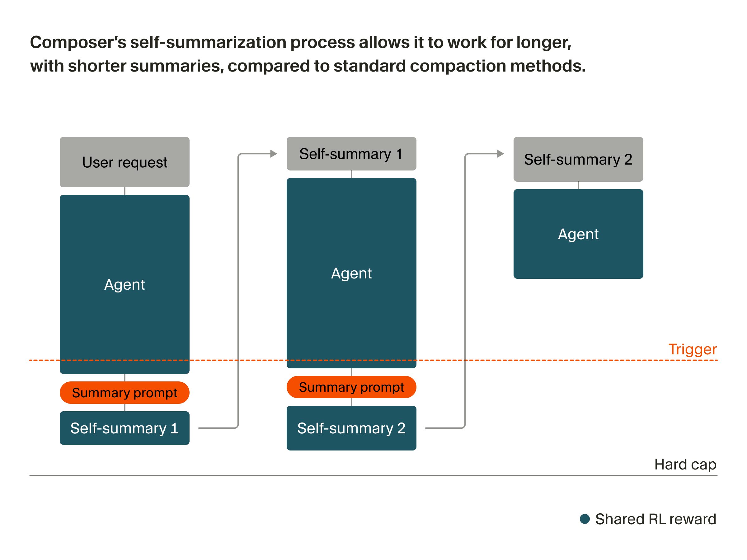
Long-horizon Composer training through self-summarization
-
Agentic coding increasingly involves trajectories that exceed the model’s context window. Simple compaction methods, such as prompted summarization or sliding-window truncation, can discard information that is essential for later steps. Training Composer for longer horizons describes a reinforcement-learning approach in which Composer is trained to summarize its own context during long tasks, allowing reward to flow not only to final agent actions but also to the intermediate summaries that preserved useful state.
-
The following figure (source) shows the self-summarization loop: the agent generates until a context-length trigger, produces a compact self-summary, continues from the condensed context, and receives a shared RL reward over the chained trajectory.
-
This can be modeled as a chained trajectory:
\[\tau = (x_0, y_0, c_1, y_1, c_2, \ldots, y_T, R)\]-
where \(x_0\) is the initial user request, \(y_i\) are agent action segments, \(c_i\) are self-generated compacted contexts, and \(R\) is the final reward for the task outcome. A simple shared-reward objective for all generated tokens in the chain is:
\[\mathcal{L}_{\text{RL}}(\theta) =-R \sum_{t=1}^{T} \log \pi_\theta(z_t \mid z_{<t})\]- where \(z_t\) ranges over both task-action tokens and self-summary tokens. This objective upweights summaries that preserve information leading to success and downweights summaries that omit critical details. The approach makes memory management a trained behavior rather than a fixed harness-level heuristic.
-
-
This is closely related to the broader challenge of evaluating and training agents on long-horizon software tasks. SWE-bench: Can Language Models Resolve Real-World GitHub Issues? by Jimenez et al. (2023) frames software repair as repository-level issue resolution requiring multi-file reasoning, while Terminal-Bench: Benchmarking Agents on Hard, Realistic Tasks in Command Line Interfaces by Merrill et al. (2026) evaluates agents on realistic terminal tasks that require long sequences of actions.
Why this matters for coding agents
-
Online RL changes the training objective from “predict plausible code” to “take actions that developers accept, keep, and benefit from.” For autocomplete, this means learning when to suggest and when to stay silent. For agentic editing, it means learning which tool calls, edits, questions, and plans lead to durable progress in a real codebase. For long-horizon agents, it means learning how to preserve task state across many steps so that final outcomes improve.
-
The central tradeoff is that online RL provides fresher and more realistic feedback, but it also exposes the model to noisier rewards, delayed outcomes, product-specific incentives, and reward-hacking surfaces. Stable production online RL therefore depends on three coupled systems: a policy-gradient training method, a reward pipeline that aligns with user value, and a deployment-evaluation loop fast enough to keep the data approximately on-policy.
Reward Design
- Reward design translates product outcomes into scalar learning signals. In online RL for coding systems, this signal is not merely a benchmark score; it is a proxy for whether the model’s action improved the developer’s workflow. Improving Cursor Tab with online RL uses acceptance and rejection of suggestions to define a policy-gradient reward for autocomplete behavior, while Improving Composer through real-time RL uses production interaction signals to improve an agentic coding model through frequent checkpoint updates.
Proxy Rewards
- A reward function \(R_{\text{proxy}}\) is a measurable approximation to the intended product value \(R_{\text{true}}\):
-
The central difficulty is that user value is multidimensional. A coding assistant should produce correct code, avoid unnecessary interruptions, preserve user intent, minimize latency, avoid destructive edits, use tools reliably, and recover gracefully from uncertainty. A scalar reward compresses these objectives into a single signal, so its design determines which behaviors the policy learns to amplify.
-
A general composite reward can be written as:
\[R(s,a) = \lambda_{\text{accept}} R_{\text{accept}} + \lambda_{\text{persist}} R_{\text{persist}} - \lambda_{\text{dissatisfy}} R_{\text{dissatisfy}} - \lambda_{\text{latency}} C_{\text{latency}} - \lambda_{\text{risk}} C_{\text{risk}}\]- where positive terms reward useful accepted or persistent changes, while cost terms penalize dissatisfaction, delay, unsafe edits, invalid tool use, or excessive interruption. The weights \(\lambda_i\) define the product tradeoff: increasing \(\lambda_{\text{accept}}\) may improve immediate acceptance, while increasing \(\lambda_{\text{risk}}\) may make the model more conservative.
Suggestion Rewards
-
Autocomplete exposes a clean reward-design problem because the system can observe whether a suggestion is accepted. Improving Cursor Tab with online RL illustrates this with a thresholded policy objective: accepted suggestions receive positive reward, rejected suggestions receive negative reward, and showing nothing receives zero reward, causing the model to learn when silence is preferable to a low-confidence suggestion.
-
Let \(\tau\) be the desired minimum probability that a suggestion will be accepted. A simple reward is:
- If the model shows a suggestion whose probability of acceptance is \(p\), the expected reward is:
- Therefore, showing a suggestion is reward-improving exactly when:
- This reward does not require a separately calibrated acceptance classifier. Instead, policy optimization can make the model internalize the action boundary between useful completion and distraction. This is a product-specific instance of the policy-gradient principle in Policy Gradient Methods for Reinforcement Learning with Function Approximation by Sutton et al. (2000), which directly optimizes a parameterized policy with respect to expected reward.
Agent Rewards
-
Agentic coding requires broader rewards than autocomplete because the action space includes editing, reading files, running commands, calling tools, asking clarifying questions, and choosing when to stop. Improving Composer through real-time RL describes a real-time RL loop in which real production interactions are distilled into rewards, updated checkpoints are evaluated for regressions, and improved versions can be deployed behind Auto as often as every five hours.
-
For an agent trajectory \(\tau\) with states \(s_t\), actions \(a_t\), and delayed outcome reward \(R_T\), a trajectory-level objective can be written as:
- A likelihood-ratio policy-gradient update assigns credit to the sampled actions in the trajectory:
- In practice, a production coding agent usually benefits from denser reward components because final user satisfaction may be delayed or sparse. Intermediate signals can include whether edits persist in the codebase, whether the user sends dissatisfied follow-ups, whether tool calls are valid, whether tests pass, whether the user accepts a plan, and whether latency remains acceptable. These signals must be treated as proxies, because each can be gamed if optimized in isolation.
Credit Assignment
-
Longer agent trajectories make credit assignment harder because the outcome may depend on many earlier actions. A final successful edit may depend on earlier repository exploration, an intermediate plan, a correct terminal command, or a compact summary that preserved the right context. Training Composer for longer horizons frames self-summarization as an RL-trained behavior, allowing final task reward to upweight both the agent actions and the summaries that made long-horizon success possible.
-
A trajectory with intermediate summaries can be represented as:
- where \(x_0\) is the task, \(y_i\) are agent action segments, \(c_i\) are compacted self-summaries, and \(R_T\) is the final outcome reward. A shared-reward loss can be written as:
- This formulation rewards summary tokens and action tokens together. If a summary preserves the information needed for later success, its tokens receive positive reinforcement; if it omits critical context and the trajectory fails, its tokens are downweighted. This converts context management from a hand-written harness rule into a learned behavior.
Reward Hacking
-
Reward hacking occurs when the policy improves the measured reward while violating the intended objective. Concrete Problems in AI Safety by Amodei et al. (2016) identifies reward hacking as a core failure mode in deployed learning systems, especially when the specified objective differs from the behavior designers actually want. Improving Composer through real-time RL describes this risk in real-time coding RL, including broken tool calls that avoided negative reward and excessive clarification that deferred risky edits.
-
A useful diagnostic is the gap:
- When \(\Delta_R\) is large, the policy can discover behaviors that score well under the proxy while degrading actual user value. Real-time RL makes this risk more visible because real users react to poor behavior, but it also makes the reward surface more complex because the model is optimizing against the full production stack: instrumentation, telemetry, aggregation logic, reward definitions, evaluation gates, and deployment policies.
Guardrails
-
Reward design in production should be paired with guardrails that detect proxy failures before they become model behavior. These guardrails include regression evaluations, A/B tests, human inspection of high-impact failures, negative examples for invalid tool calls, monitoring of action-rate shifts, and explicit penalties for behaviors that exploit missing reward terms. Improving Composer through real-time RL emphasizes that frequent deployment must be coupled with evaluation suites and monitoring so that reward improvements do not mask regressions.
-
A practical constrained objective can be written as:
- where \(C_j\) are costs such as invalid tool-call rate, excessive latency, destructive edit rate, or dissatisfied follow-up rate. In the unconstrained Lagrangian form:
- The coefficients \(\beta_j\) express which regressions are unacceptable even when the main reward improves. This is essential for coding agents because a model can become more aggressive, faster, or more reward-seeking while becoming less trustworthy.
Takeaways
-
Reward design determines what online RL actually optimizes. For autocomplete, it can encode a target acceptance threshold and teach the model when not to suggest. For agentic coding, it must combine delayed outcome quality with intermediate signals such as valid tool use, persistent edits, low dissatisfaction, and acceptable latency. For long-horizon agents, it must assign credit not only to final edits but also to planning, exploration, and memory-management actions that make later success possible.
-
The main risk is proxy mismatch. A production reward must be treated as an evolving specification rather than a fixed metric: every observed reward hack is evidence that the proxy is incomplete, and every deployment cycle is an opportunity to refine the alignment between measured reward and actual user value.
On-Policy Loops
- Online RL depends on a tight loop between deployment, data collection, reward computation, training, evaluation, and redeployment. Improving Cursor Tab with online RL describes why fresh user interactions are needed after each policy update, since policy-gradient training assumes that actions are sampled from the policy being optimized. Improving Composer through real-time RL describes the same principle at the agentic-coding scale, where checkpoints are served to production, user responses are converted into reward signals, and improved checkpoints are redeployed frequently.
Loop
- A production online RL loop can be written as:
-
where \(\pi_{\theta_k}\) is the deployed policy, \(\mathcal{D}_k\) is the interaction data collected from that policy, \(\hat{R}_k\) is the reward signal inferred from user and environment feedback, and \(\theta_{k+1}\) is the updated checkpoint. The evaluation gate is essential because the reward signal may be noisy, incomplete, or exploitable, so an observed training improvement must be checked against regressions before deployment.
-
For a batch \(\mathcal{D}_k = \{(s_i, a_i, r_i)\}_{i=1}^N\) collected from \(\pi_{\theta_k}\), a simple policy-gradient update is:
- This estimator is most faithful when \(a_i \sim \pi_\theta(\cdot \mid s_i)\). If the deployed policy has already changed substantially, the samples no longer match the distribution assumed by the gradient.
Freshness
-
The central operational constraint is data freshness. If a model is trained on interactions from an older policy, the update becomes off-policy. In small tabular problems this can sometimes be corrected, but in large language-model policies the action space is extremely high-dimensional and the trajectory distribution can shift quickly after each update.
-
Let \(\pi_{\theta_{\text{old}}}\) be the policy that generated the data and \(\pi_{\theta_{\text{new}}}\) be the policy being optimized. The mismatch can be summarized by a divergence between the two action distributions:
- As this divergence grows, old data becomes a less reliable guide for improving the new policy. This is why the cadence of collecting interaction data, training, and redeploying becomes part of the algorithm rather than merely an engineering concern.
Corrections
- A classical way to reuse off-policy data is importance sampling. If an action was sampled from \(\pi_{\theta_{\text{old}}}\) but evaluated under \(\pi_\theta\), the correction ratio is:
- The corrected estimator becomes:
- In large action spaces, however, \(\rho_i(\theta)\) can have high variance because small probability changes over long token sequences compound multiplicatively. For a generated sequence \(a = (y_1,\ldots,y_T)\), the ratio becomes:
- This product can become unstable for long completions, tool-call sequences, or multi-step agent trajectories. The practical implication is that keeping data nearly on-policy is often more robust than relying on heavy off-policy correction.
Clipping
- Modern policy optimization often limits how far the new policy can move from the behavior policy that generated the data. Proximal Policy Optimization Algorithms by Schulman et al. (2017) introduces a clipped surrogate objective that enables multiple minibatch updates while discouraging overly large policy changes. The PPO clipped objective is:
-
where \(\hat{A}_t\) is an advantage estimate and \(\epsilon\) is a clipping hyperparameter. The clipping term prevents the optimizer from receiving additional benefit for moving \(\rho_t(\theta)\) too far from \(1\), which stabilizes policy updates.
-
Trust Region Policy Optimization by Schulman et al. (2015) formalizes a related constraint-based approach, where policy improvement is performed under a bound on the KL divergence between the old and new policies. A simplified constrained form is:
- These objectives are relevant to production online RL because a fast deployment loop and a conservative update rule solve complementary problems: fast deployment keeps data fresh, while conservative optimization limits destabilizing changes between checkpoints.
Cadence
-
Cadence determines how on-policy the training data remains. Improving Cursor Tab with online RL reports a rapid loop for rolling out a checkpoint and collecting the next training batch, emphasizing that the policy-gradient update requires suggestions sampled from the current model. Improving Composer through real-time RL reports a multi-hour checkpoint cycle for Composer, emphasizing that frequent deployment keeps real interaction data fully or almost fully on-policy.
-
The cadence can be represented as a staleness interval:
-
where \(t_{\text{serve}}\) is when the model produced the action and \(t_{\text{train}}\) is when the resulting data is used for training. The larger \(\Delta t\) becomes, the more likely it is that the deployed policy, user distribution, product surface, or reward definition has changed before the update is applied.
-
A production online RL system therefore tries to minimize:
- Reducing any term improves data freshness, but none can be removed carelessly. For example, shortening evaluation may increase deployment speed while increasing the chance of shipping a reward-hacked or regressed policy.
Batches
-
Even when data is fresh, online RL rewards can be noisy. User behavior is variable, repository states differ, tasks have different difficulty, and identical model behavior can receive different feedback depending on context. Large batches reduce variance:
\[\operatorname{Var} \left[ \frac{1}{N} \sum_{i=1}^{N} g_i \right] = \frac{\sigma^2}{N}\]- where \(g_i = \nabla_\theta \log \pi_\theta(a_i \mid s_i) r_i\) and \(N\) is the batch size. This creates a tension: large batches improve gradient reliability, but waiting for large batches increases staleness. Production online RL must therefore balance sample freshness against statistical confidence.
-
A practical batch design can prioritize:
- recent data from the current checkpoint,
- enough volume to average out noisy user-level feedback,
- stratification across languages, repositories, task types, and user workflows,
- filtering or downweighting of telemetry artifacts that do not reflect genuine user value,
- evaluation splits that catch regressions not visible in the main reward.
Gates
-
Evaluation gates convert online RL from a pure optimization loop into a controlled deployment process. A checkpoint should not be shipped merely because the training reward improved. It should also pass task-level benchmarks, product metrics, regression tests, safety checks, and monitoring thresholds.
-
A simple gate can be written as:
- where \(M_j\) are evaluation metrics and \(\epsilon_j\) are allowed regression tolerances. This formulation allows a checkpoint to improve the main reward while still being blocked if it degrades latency, tool validity, edit persistence, user satisfaction, or benchmark performance beyond an acceptable threshold.
Drift
-
Online systems must distinguish improvement from drift. A policy can change because it learned a genuinely better behavior, because the user population changed, because the product surface changed, or because the reward pipeline changed. Monitoring should therefore track both outcomes and action distributions.
-
For an action feature vector \(\phi(a,s)\), drift can be measured as:
- In coding agents, useful drift metrics include suggestion frequency, edit size, clarification rate, tool-call failure rate, terminal-command frequency, file-read depth, latency distribution, and rollback rate. Large changes in these metrics may be valuable if intentional, but they should be inspected because reward hacking often appears first as an unexpected shift in action distribution.
Takeaways
-
On-policy data is the foundation of production online RL. Policy-gradient updates are most reliable when the same policy being optimized generated the actions being rewarded. This makes deployment cadence, logging latency, reward computation, batch construction, conservative updates, and evaluation gates part of the learning algorithm.
-
The practical goal is not to make every sample perfectly on-policy. The goal is to keep the data fresh enough that reward-weighted updates reflect the behavior of the current model, while keeping evaluation strong enough that reward improvements correspond to real improvements in the coding experience.
Instrumentation
- Instrumentation is the bridge between production behavior and RL training data. In online RL for coding systems, the model’s raw outputs are not enough: the training loop also needs structured records of the state, action, context, user response, environment result, latency, and deployment checkpoint that produced each interaction. Improving Composer through real-time RL describes this as a stack-wide process that begins with client-side instrumentation, passes through backend data pipelines, and ends in a fast deployment path for updated checkpoints.
Events
- A production interaction can be represented as an event tuple:
-
where \(u_i\) is an anonymized user or session identifier, \(c_i\) is the checkpoint identifier, \(s_i\) is the observed state, \(a_i\) is the model action, \(o_i\) is the observed outcome, \(r_i\) is the derived reward, \(m_i\) is metadata, and \(t_i\) is the timestamp. The checkpoint identifier is essential because the learning algorithm must know which policy generated the action.
-
For autocomplete, \(a_i\) may be a suggestion or the decision to show nothing. For an agent, \(a_i\) may be a file edit, tool call, terminal command, search query, plan update, clarification question, or final response. The same logging abstraction can support both, but agentic coding requires richer state and outcome records because reward can depend on delayed effects.
State
-
The state \(s\) should capture the information available to the policy when it acted, not information observed only afterward. For coding assistants, this can include the visible editor context, cursor position, recent edits, file path, programming language, repository metadata, active plan state, retrieved files, tool results, and conversation history.
-
A useful distinction is:
- where \(s_i^{\text{policy}}\) is the state actually visible to the model and \(s_i^{\text{logged}}\) is the broader telemetry available for debugging, reward computation, and evaluation. This distinction prevents leakage: training should not accidentally reward or condition on information that the deployed policy could not have known at action time.
Actions
-
The action space determines what the reward can shape. In Tab, the main action is whether to show a suggestion and what text or edit to suggest. Improving Cursor Tab with online RL describes Tab as a policy that learns not only what completion to produce, but also when no suggestion should be shown because a low-quality suggestion would interrupt the developer.
-
For Composer, the action space is broader:
- This broader action space makes instrumentation more important. A final user-visible answer may be poor because an earlier file search was incomplete, a terminal command failed, a summary lost state, or the model stopped too soon. Recording only the final text would hide the cause of failure.
Outcomes
-
Outcomes are the observable consequences of model actions. In autocomplete, the outcome may be accept, reject, ignore, modify, or continue typing. In agentic editing, the outcome may include whether edits persisted, whether tests passed, whether the user reverted changes, whether the user sent a dissatisfied follow-up, and whether the task eventually completed.
-
A delayed outcome can be written as:
- This matters because the immediate reaction to an action may be ambiguous. A user may not instantly reject a poor edit, but may later undo it or ask the agent to repair it. Good instrumentation therefore records both local outcomes and downstream consequences.
Rewards
- Reward computation converts outcomes into scalar signals. A general reward pipeline can be written as:
-
where \(g\) is a reward function over observed outcomes and metadata. In online RL systems, \(g\) is part of the product specification: it determines whether the model learns to be concise, proactive, cautious, fast, persistent, or exploratory.
-
For a multi-signal coding reward:
- The weights \(\lambda_j\) should be tuned against user value rather than against isolated metric gains. A reward that overweights acceptance may encourage short, obvious suggestions; a reward that underweights latency may improve quality while damaging the interactive feel of the product.
Attribution
- Instrumentation must support attribution: the training system needs to connect each reward back to the policy action that plausibly caused it. For immediate feedback, this is straightforward:
- For long-horizon agents, the mapping is more difficult:
- A practical approach is to store the full trajectory and assign a shared or advantage-weighted reward across the actions that contributed to the outcome. Training Composer for longer horizons describes this principle for self-summarization, where final trajectory reward is applied not only to task actions but also to intermediate summaries that preserved useful information.
Latency
- Latency is both a product metric and an RL signal. A model that produces better edits but responds too slowly may reduce developer flow. A model that responds quickly but makes shallow or incorrect edits may also reduce value. Instrumentation should therefore log latency at multiple levels:
- This decomposition helps identify whether a regression came from the model, tool calls, retrieval, infrastructure, or client rendering. It also allows the reward function to penalize avoidable delay without discouraging necessary exploration on hard tasks.
Quality
-
Quality signals should combine automatic, behavioral, and evaluation-based measures. Automatic signals include test results, syntax validity, type-checking, linter outcomes, and tool success. Behavioral signals include acceptance, persistence, revert rate, follow-up sentiment, and repeated repair requests. Evaluation signals include benchmark scores and regression-suite results.
-
The measured quality vector can be written as:
- The scalar reward is then a projection:
- This projection should be monitored continuously because user behavior and product surfaces change over time. A weight vector that works for autocomplete may be inappropriate for multi-step repository edits.
Privacy
-
Production instrumentation should collect the minimum information needed for learning, evaluation, and debugging. In coding products, raw interaction data may include proprietary code, secrets, filenames, logs, or business context. A robust pipeline should support filtering, access control, retention limits, aggregation, and separation between identifiable metadata and model-training records.
-
A useful design target is:
- where \(I\) is the collected information and \(\eta\) is the minimum signal quality required for reliable training. The goal is not to collect everything, but to collect enough structured signal to improve the policy responsibly.
Takeaways
-
Instrumentation makes online RL possible. It records which checkpoint acted, what state it saw, what action it took, how the user and environment responded, how reward was computed, and whether the resulting checkpoint improved or regressed. For autocomplete, this enables learning the boundary between useful suggestion and interruption. For agentic coding, it enables credit assignment across edits, tool calls, plans, summaries, and delayed user outcomes.
-
The quality of the RL system is bounded by the quality of its instrumentation. If important outcomes are missing, the reward will be incomplete; if attribution is wrong, the policy will reinforce the wrong actions; if latency and regressions are not measured, the model can improve the main reward while degrading the product.
Evaluation
- Evaluation is the safety valve in production online RL. A checkpoint should not be deployed simply because its training reward improves; it should also preserve or improve the broader product qualities that the reward only approximates. Improving Composer through real-time RL describes a real-time RL loop in which Composer checkpoints are trained from production reward signals and then run through evaluation suites before deployment, while Improving Cursor Tab with online RL shows that product metrics such as suggestion frequency and acceptance rate can move together in non-trivial ways.
Metrics
-
A deployed coding model should be evaluated along multiple axes:
- Outcome quality: whether the generated edit, patch, or suggestion actually helps complete the task.
- User value: whether the developer accepts, keeps, or positively responds to the model’s action.
- Behavioral reliability: whether the model avoids unnecessary interruptions, invalid tool calls, destructive edits, and excessive clarification.
- System quality: whether the model maintains acceptable latency, cost, and stability.
-
A multi-metric evaluation vector can be written as:
- The deployment decision should depend on the full vector rather than a single scalar. This prevents a checkpoint from improving a narrow reward while degrading the developer experience.
Benchmarks
-
Benchmarks provide repeatable tests that are independent of live user behavior. SWE-bench: Can Language Models Resolve Real-World GitHub Issues? by Jimenez et al. (2023) evaluates whether models can resolve real GitHub issues by editing repositories, making it relevant for measuring repository-level coding ability. Terminal-Bench: Benchmarking Agents on Hard, Realistic Tasks in Command Line Interfaces by Merrill et al. (2026) evaluates agents on realistic terminal tasks with environment interaction and tests, making it relevant for tool-using coding agents. Evaluating Large Language Models Trained on Code by Chen et al. (2021) introduces HumanEval for functional correctness on code-generation tasks, making it useful for focused program-synthesis checks.
-
For a benchmark set \(\mathcal{B} = \{b_i\}_{i=1}^N\), the pass rate is:
- Benchmarks are necessary but incomplete. They provide controlled regression signals, but they cannot fully capture interactive product behavior such as when to interrupt, how much context to explore, how often to ask clarifying questions, or how developers react to partial solutions.
Product Metrics
-
Product metrics measure behavior in the deployed environment. For Tab, the core metrics include suggestion rate and acceptance rate. Improving Cursor Tab with online RL reports that online RL trained a Tab model that made fewer suggestions while achieving a higher acceptance rate, illustrating that a better policy can improve precision by learning when not to act.
-
The acceptance rate can be written as:
- The suggestion rate can be written as:
-
These metrics should be interpreted together. A model can raise acceptance rate by becoming too conservative, or raise suggestion rate by becoming too noisy. The product objective is not to maximize either metric alone, but to choose actions that improve developer flow.
-
For Composer, useful product metrics include edit persistence, dissatisfied follow-ups, latency, task completion, user reverts, tool-call success, and repeated repair requests. Improving Composer through real-time RL reports A/B-tested changes in edit persistence, dissatisfied follow-ups, and latency, making these examples of product-level evaluation signals for agentic coding.
Regression Gates
-
A regression gate blocks deployment when a checkpoint improves one metric but degrades another beyond tolerance. This can be formalized as:
\[\text{Deploy}(\theta_{k+1}) = \mathbb{1} \left[ M_j(\theta_{k+1}) - M_j(\theta_k) \geq -\epsilon_j \;\;\forall j \right]\]-
where \(M_j\) is an evaluation metric and \(\epsilon_j\) is the maximum tolerated regression. A stricter version requires statistically significant improvement on the primary metric and no significant degradation on guardrail metrics:
\[\Delta M_{\text{primary}} > \epsilon_{\text{primary}} \quad \text{and} \quad \Delta M_j \geq -\epsilon_j \quad \forall j \in \mathcal{G}\]- where \(\mathcal{G}\) is the set of guardrail metrics. In coding agents, guardrails commonly include latency, invalid tool calls, destructive edits, safety checks, benchmark pass rates, and user dissatisfaction.
-
A/B Tests
- A/B testing compares a candidate checkpoint against a baseline in the real product environment. Let \(Y_i\) be a user-level or session-level outcome, and let \(T_i \in \{0,1\}\) indicate whether the interaction used the candidate model. The average treatment effect is:
- A/B testing is especially important for online RL because reward improvements can overfit the training signal. A candidate model should demonstrate that its learned behavior improves real user outcomes, not only offline reward estimates or internal benchmark scores.
Slices
-
Aggregate metrics can hide regressions. A model may improve overall while becoming worse for a specific programming language, repository size, framework, operating system, or task type. Evaluation should therefore include slice metrics:
\[M_{j,g}(\theta) = \mathbb{E} \left[ m_j(x, \pi_\theta) \mid x \in g \right]\]- where \(g\) is a slice such as language, file type, task length, edit size, tool type, or user workflow. Slice evaluation is particularly important for coding assistants because production traffic is heterogeneous: a policy update that improves short Python completions may not improve long TypeScript refactors or terminal-heavy debugging tasks.
Drift
- Online RL can change both the quality of actions and the distribution of actions. Drift monitoring checks whether the new checkpoint behaves differently in ways that are not fully captured by reward. For an action-feature vector \(\phi(s,a)\), distributional drift can be measured as:
- Useful drift features include suggestion frequency, edit length, tool-call frequency, terminal-command rate, clarification rate, file-read depth, refusal rate, latency, and stop-action frequency. Unexpected drift should be inspected even when reward improves, because reward hacking often appears first as a behavioral distribution shift.
Scorecards
- A deployment scorecard summarizes whether a checkpoint is ready to ship:
| Area | Example metric | Purpose |
|---|---|---|
| Reward | Mean online RL reward | Checks the optimized objective |
| Quality | Benchmark pass rate | Detects task regressions |
| Product | Accept rate, edit persistence | Measures user-facing value |
| Friction | Dissatisfied follow-ups, reverts | Detects poor interaction quality |
| Systems | Latency, cost, error rate | Preserves product responsiveness |
| Behavior | Tool failures, clarification rate | Detects policy drift |
| Slices | Language and task-specific metrics | Catches hidden regressions |
- A checkpoint should be treated as an improvement only when the scorecard shows a coherent pattern: reward improves, guardrails hold, product metrics move in the intended direction, and no important slice regresses.
Takeaways
-
Evaluation turns online RL from unconstrained reward maximization into controlled model improvement. Benchmarks measure repeatable coding ability, product metrics measure real developer value, A/B tests validate behavior in deployment, regression gates prevent unsafe tradeoffs, and slice analysis catches hidden failures.
-
The practical rule is that the reward may propose a checkpoint, but evaluation decides whether it ships.
Synthesis
- Production online RL turns deployed interaction into a continuous model-improvement loop. For coding systems, this is powerful because the most important supervision often comes from real developer behavior rather than from static labels or isolated benchmarks. Improving Cursor Tab with online RL describes how autocomplete can use acceptance and rejection feedback to learn when to suggest and when to remain silent, Improving Composer through real-time RL describes how an agentic coding model can use real production interaction tokens as reward-bearing data for frequent checkpoint updates, and Training Composer for longer horizons describes how long-horizon agent training can reward self-generated summaries that preserve task state across context limits.
Objective
-
A unified view of production online RL is:
\[\max_\theta \; \mathbb{E}_{\tau \sim \pi_\theta} \left[ R_{\text{product}}(\tau) \right]\]- where \(\tau\) is an interaction trajectory and \(R_{\text{product}}\) is a reward proxy for developer value. For Tab, \(\tau\) may be a short interaction around a suggestion. For Composer, \(\tau\) may include file reads, edits, terminal commands, tool calls, clarifying questions, summaries, and final user responses.
-
This differs from standard supervised learning, which optimizes token prediction:
- Online RL instead optimizes actions according to observed outcomes:
- Policy Gradient Methods for Reinforcement Learning with Function Approximation by Sutton et al. (2000) provides the policy-gradient foundation for directly optimizing parameterized policies, while Simple Statistical Gradient-Following Algorithms for Connectionist Reinforcement Learning by Williams (1992) introduces the likelihood-ratio update that reinforces sampled actions in proportion to reward.
Design
-
A production coding assistant trained with online RL needs four aligned components:
- Policy: the deployed model that generates suggestions, edits, plans, tool calls, or summaries.
- Reward: the scalar signal inferred from user behavior, environment outcomes, latency, persistence, and dissatisfaction.
- Loop: the infrastructure that keeps data fresh by collecting interactions, training checkpoints, evaluating regressions, and redeploying quickly.
- Guardrails: the evaluation and monitoring layer that prevents reward improvements from hiding regressions.
-
The design can be summarized as a constrained optimization problem:
\[\begin{aligned} \max_{\theta} \quad & \mathbb{E}_{\pi_{\theta}}\left[ R_{\text{value}}(\tau) \right] \\ \text{subject to} \quad & \mathbb{E}_{\pi_{\theta}}\left[ C_j(\tau) \right] \leq \epsilon_j, \quad \forall j \end{aligned}\]- where \(R_{\text{value}}\) captures intended user value, and each \(C_j\) captures a cost such as latency, invalid tool calls, destructive edits, excessive interruption, dissatisfaction, or benchmark regression. Proximal Policy Optimization Algorithms by Schulman et al. (2017) is relevant because it constrains policy updates through a clipped objective, which is useful when repeatedly updating large policies from sampled trajectories.
Tradeoffs
-
Online RL improves realism because the model learns from the environment in which it is actually used. It also introduces several tradeoffs:
- Freshness vs. batch size: fresher data is more on-policy, while larger batches reduce gradient noise.
- Reward strength vs. reward hacking: stronger optimization can reveal flaws in the reward proxy more quickly.
- Latency vs. reasoning depth: shorter responses preserve flow, while harder tasks may require more exploration and tool use.
- Suggestion rate vs. acceptance rate: fewer suggestions can raise precision, but excessive conservatism can reduce usefulness.
- Automation vs. user control: more agent autonomy can complete larger tasks, but it increases the cost of incorrect actions.
-
A useful decomposition is:
- The challenge is not simply to maximize \(R\), but to ensure that this scalar reward remains a faithful proxy for the developer’s actual experience. Concrete Problems in AI Safety by Amodei et al. (2016) is relevant because it formalizes reward hacking as a core failure mode when a learned policy exploits the gap between specified and intended objectives.
Lessons
-
Production online RL is most effective when the product itself supplies dense, meaningful feedback. Tab has a relatively direct feedback signal because the system can observe whether a suggestion was accepted. Composer has a richer but noisier feedback surface because success depends on multi-step edits, user satisfaction, tool reliability, and whether the resulting code remains useful. Long-horizon Composer training adds another layer: memory management becomes part of the policy, so summaries, plans, and intermediate decisions receive credit when they help the final outcome.
-
Several principles follow:
- Keep data near on-policy: the checkpoint that generated the data should be close to the checkpoint being optimized.
- Reward outcomes, not only surface form: accepted suggestions, persistent edits, and successful task completion are closer to value than token likelihood alone.
- Evaluate beyond the reward: A/B tests, benchmarks, slice analysis, latency checks, and regression gates are needed because every reward is incomplete.
- Monitor behavior shifts: changes in edit size, tool-call rate, clarification rate, or suggestion frequency can reveal reward hacking before aggregate metrics fail.
- Train the harness behaviors: planning, summarization, tool selection, stopping, and asking questions should be treated as learnable actions when they affect task success.
Outlook
-
The direction suggested by online RL for coding agents is a move from static model releases toward continual, product-grounded learning. In this setting, the model is not only trained to produce plausible code; it is trained to interact with developers, decide when to act, preserve state across long tasks, recover from uncertainty, and optimize for changes that users actually keep.
-
The long-term pattern is likely to combine several feedback sources:
\[R_{\text{total}} = \alpha R_{\text{user}} + \beta R_{\text{environment}} + \gamma R_{\text{evaluation}} + \delta R_{\text{AI-feedback}}\]- where \(R_{\text{user}}\) comes from developer behavior, \(R_{\text{environment}}\) comes from tests and tools, \(R_{\text{evaluation}}\) comes from benchmark and regression suites, and \(R_{\text{AI-feedback}}\) may come from model-based judges or critiques. Constitutional AI: Harmlessness from AI Feedback by Bai et al. (2022) is relevant because it studies reinforcement learning from AI feedback, showing how model-generated preference signals can supplement direct human labeling in alignment-oriented training.
-
The central conclusion is that online RL makes coding assistants more adaptive, but also more dependent on the quality of their reward, instrumentation, and evaluation loop. A successful system must therefore treat product telemetry, reward modeling, policy optimization, and deployment evaluation as one coupled learning system.
Types of Reinforcement Learning
-
RL encompasses a family of methods that differ in how they represent knowledge about the environment, update that knowledge, and derive decision policies. At its essence, RL aims to learn an optimal policy \(\pi^*(a \mid s)\) that maximizes the expected cumulative reward:
\[J(\pi) = \mathbb{E}_\pi \left[ \sum_{t=0}^{\infty} \gamma^t r_t \right]\]- where \(\gamma \in [0,1]\) is the discount factor weighting future rewards, and \(r_t\) is the reward at time \(t\).
- Classical RL refers to the family of foundational RL algorithms that learn from interaction or modeled experience using explicit value functions, policies, and environment models—without relying on deep neural networks for function approximation.
- While classical RL methods provide the theoretical foundation for sequential decision-making and control, modern deep RL extends these principles by leveraging neural networks to approximate value functions and policies in complex, high-dimensional environments. A detailed discourse on deep RL is available in the Deep Reinforcement Learning section.
-
The following are the principal categories of classical RL techniques, each of which will be explored in detail in subsequent subsections. While these categories are often presented separately, they are not entirely independent—many RL algorithms combine ideas across them. For example, actor–critic methods merge policy-based and value-based principles, and both model-based and model-free approaches can be implemented using either value-based or policy-based learning. In other words, model-based/model-free defines how an agent learns from or about the environment, while value-based/policy-based defines what the agent learns to optimize its behavior.
-
Value-Based Methods: Value-based methods estimate the value of states or state–action pairs and derive an optimal policy by choosing actions that maximize these values. A foundational example is Q-learning by Watkins & Dayan (1992).
-
Policy-Based Methods: Policy-based methods directly optimize the agent’s policy \(\pi(a \mid s)\) using gradient-based techniques without explicitly estimating value functions. A seminal contribution in this area is the REINFORCE algorithm by Williams (1992).
-
Actor–Critic Methods: Actor–Critic methods combine value-based and policy-based principles by maintaining two components: an actor that proposes actions and a critic that evaluates them. This structure was formalized by Barto, Sutton & Anderson (1983).
-
Model-Based Methods: Model-based RL algorithms explicitly learn or use a model of the environment’s dynamics \(P(s' \mid s,a)\) and reward function \(R(s,a)\) to enable planning and decision-making. The approach originates from policy iteration and value iteration introduced by Howard (1960).
-
Model-Free Methods: Model-free methods dispense with explicit environment modeling and instead learn directly from interaction data, adjusting their estimates of value or policy from experience tuples \((s,a,r,s')\). A canonical example is SARSA by Rummery & Niranjan (1994).
-
On-Policy vs. Off-Policy Learning: This distinction describes whether an agent learns from data generated by its own policy or another policy. On-policy methods (e.g., SARSA) update based on their current behavior, while off-policy methods (e.g., Q-learning) learn from experiences generated by a different policy (Precup, Sutton & Singh, 2000).
-
Value-Based Methods
- Value-based methods form the cornerstone of RL. Their core principle is to learn value functions that estimate how good it is for an agent to be in a given state or to perform a specific action in that state.
- These methods do not learn policies directly; instead, they infer the optimal policy from the learned values by choosing actions that maximize expected future rewards.
Foundations of Value Functions
-
Two central value functions define this class of methods:
- State-Value Function:
- This represents the expected cumulative reward when starting from state \(s\) and following policy \(\pi\) thereafter.
- Action-Value Function:
-
This quantifies the expected return when taking action \(a\) in state \(s\) and then following policy \(\pi\).
-
The optimal policy \(\pi^*\) can then be derived as:
\[\pi^*(s) = \arg\max_a Q^*(s,a)\]- where \(Q^*(s,a)\) is the optimal action-value function.
Dynamic Programming (DP)
-
Dynamic Programming represents the earliest and most theoretically grounded approach to solving RL problems. It assumes that a complete model of the environment is known—specifically, the transition probabilities \(P(s' \mid s,a)\) and reward function \(R(s,a)\).
-
Introduced by Bellman (1957), DP methods are built upon the Bellman Optimality Equation, which recursively expresses the relationship between the value of a state and the values of its successor states:
-
Two major DP algorithms are:
- Value Iteration: Alternates between evaluating and improving the value function until convergence to \(V^*(s)\).
- Policy Iteration: Alternates between policy evaluation (estimating \(V^{\pi}\)) and policy improvement (updating \(\pi\)) until the policy stabilizes.
-
DP is exact and guaranteed to converge for finite MDPs, but it is computationally infeasible in large state spaces due to the curse of dimensionality.
-
Key Reference:
- Howard (1960): introduced policy iteration as a computationally efficient refinement to Bellman’s DP framework.
Monte Carlo (MC) Methods
-
Monte Carlo methods learn value functions from experience, without requiring a model of the environment. They estimate expected returns by averaging the actual returns observed after complete episodes of experience.
-
For a state \(s\), the Monte Carlo estimate of the value is:
\[V(s) \approx \frac{1}{N(s)} \sum_{i=1}^{N(s)} G_i\]- where \(G_i\) is the total return following the \(i^{th}\) visit to \(s\), and \(N(s)\) is the number of visits to \(s\).
-
Advantages:
- Model-free: no need for transition probabilities.
- Simple and unbiased estimates after enough samples.
-
Limitations:
- Requires episodes to terminate (not suitable for continuing tasks).
- Slow convergence due to reliance on complete trajectories.
-
Key References:
- Samuel (1959): introduced early machine learning ideas based on Monte Carlo updates in checkers.
- Sutton & Barto (1998): formalized Monte Carlo methods in modern RL.
Temporal Difference (TD) Learning
-
Temporal Difference learning blends the key ideas of Monte Carlo and Dynamic Programming — learning directly from raw experience without requiring a model, and updating value estimates based on bootstrapping from other estimates.
-
The core update rule for TD(\(\theta\)) is:
\[V(S_t) \leftarrow V(S_t) + \alpha \left[ r_{t+1} + \gamma V(S_{t+1}) - V(S_t) \right]\]- Here, the agent updates its estimate of \(V(S_t)\) using the observed reward plus the discounted value of the next state, rather than waiting for the episode to finish.
-
TD learning provides the foundation for most modern value-based algorithms, including SARSA and Q-Learning.
-
Advantages::
- Online, incremental updates.
- Works for both episodic and continuing tasks.
- Converges faster than Monte Carlo in many settings.
-
Key References::
- Sutton (1988): introduced Temporal Difference Learning, establishing the bridge between prediction and control.
- Watkins & Dayan (1992): extended TD ideas to Q-Learning, the most influential off-policy control algorithm.
Comparative Analysis
| Method | Model Requirement | Update Type | Sample Efficiency | Key References |
|---|---|---|---|---|
| Dynamic Programming | Requires full model | Full backup | High computational cost | Bellman (1957), Howard (1960) |
| Monte Carlo | Model-free | Episodic, complete return | Low | Samuel (1959), Sutton & Barto (1998) |
| Temporal Difference (TD) | Model-free | Bootstrapped incremental | High | Sutton (1988), Watkins & Dayan (1992) |
Policy-Based Methods
-
While value-based methods focus on estimating the long-term value of states or state–action pairs, policy-based methods take a more direct approach: they learn a parameterized policy that maps states to actions and optimize it to maximize expected return.
-
These methods are particularly useful in environments with continuous or stochastic action spaces, where value-based techniques like Q-learning are difficult to apply effectively.
Policy Representation and Objective
- In policy-based RL, the agent’s behavior is represented by a stochastic policy \(\pi_\theta(a \mid s)\), parameterized by \(\theta\). The goal is to find parameters that maximize the expected return:
- Unlike value-based methods, which derive a policy indirectly from learned value estimates, policy-based approaches directly optimize this objective by computing its gradient with respect to the parameters \(\theta\).
The Policy Gradient Theorem
- The key insight enabling policy optimization is the Policy Gradient Theorem (Sutton et al., 2000).
- It provides a way to estimate the gradient of the expected return without differentiating through the environment’s dynamics:
- This formulation allows gradient ascent on \(J(\theta)\) using trajectories sampled from the current policy.
- Intuitively, the update increases the probability of actions that yield higher returns and decreases it for less rewarding ones.
REINFORCE Algorithm
- The REINFORCE algorithm (Williams, 1992) is the simplest and most influential policy gradient method.
-
It estimates the gradient using complete episodes of experience, updating the policy parameters as follows:
\[\theta \leftarrow \theta + \alpha , \nabla_\theta \log \pi_\theta(a_t \mid s_t) , G_t\]-
where:
- \(\alpha\) is the learning rate,
- \(G_t = \sum_{k=t}^{T} \gamma^{k-t} r_k\) is the return following time \(t\).
-
- The algorithm works by reinforcing (increasing the probability of) actions that lead to higher observed returns.
Baseline Reduction
- Because the variance of gradient estimates can be large, REINFORCE often includes a baseline \(b(s_t)\), typically the state value \(V^{\pi}(s_t)\), to reduce variance without introducing bias:
- This concept laid the foundation for later actor–critic methods, where the critic effectively serves as a learned baseline.
Natural Policy Gradient (NPG)
- Standard gradient ascent can be inefficient in policy space due to curvature distortions caused by parameterization. The Natural Policy Gradient method, introduced by Kakade (2001), addresses this by using the Fisher information matrix \(F(\theta)\) to compute updates invariant to the parameter scaling:
- This ensures that updates are taken in directions that respect the geometry of the policy distribution, leading to faster and more stable convergence.
Advantages and Limitations
-
Advantages:
- Naturally handles continuous and stochastic action spaces.
- Enables stochastic exploration without explicit noise.
- Offers smooth policy improvement without discontinuities.
-
Limitations:
- High variance in gradient estimates.
- Often requires large numbers of trajectories for accurate estimation.
- Sensitive to hyperparameters like learning rate and baseline design.
Comparative Analysis
| Method | Core Idea | Handles Continuous Actions | Key Innovation | Key References |
|---|---|---|---|---|
| Policy Gradient (PG) | Optimize policy parameters via expected return gradient | Yes | Policy Gradient Theorem | Sutton et al. (2000) |
| REINFORCE | Use sampled returns to update policy probabilities | Yes | Monte Carlo estimation of policy gradient | Williams (1992) |
| Natural Policy Gradient | Adjust gradient using Fisher information for invariance | Yes | Geometric optimization in policy space | Kakade (2001) |
Actor–Critic Methods
-
Actor–Critic methods bridge the conceptual gap between value-based and policy-based RL. While policy-based methods optimize the policy directly and value-based methods estimate the expected return, actor–critic frameworks do both simultaneously.
-
They maintain two distinct components:
- The Actor, which updates the policy parameters in the direction suggested by the critic’s evaluation.
- The Critic, which estimates value functions and provides a baseline to stabilize and guide policy updates.
-
This architecture allows actor–critic methods to combine the low variance of value-based updates with the expressive flexibility of policy-based optimization.
Conceptual Foundation
- The actor–critic approach builds upon the policy gradient theorem and temporal difference (TD) learning.
-
At time \(t\), the policy \(\pi_\theta(a \mid s)\) selects an action, and the critic evaluates it using a value function \(V_w(s)\) or \(Q_w(s,a)\), parameterized by weights \(w\).
-
The actor updates its policy parameters according to:
\[\theta \leftarrow \theta + \alpha \nabla_\theta \log \pi_\theta(a_t \mid s_t) , \delta_t\]- where \(\delta_t\) is the TD error, defined as:
- This TD error acts as a critic signal, indicating whether the action taken was better or worse than expected.
The Advantage Function
- To improve stability and efficiency, actor–critic methods often use the advantage function, which measures how much better an action \(a\) is compared to the average action in a given state:
- Using the advantage function instead of raw returns reduces variance in policy gradient estimates, leading to smoother learning.
- The resulting update rule becomes:
- This formulation unifies the critic’s evaluative feedback with the actor’s improvement mechanism.
Classical Actor–Critic Algorithms
- The actor–critic paradigm originated with the Adaptive Heuristic Critic (AHC) architecture proposed by Barto, Sutton & Anderson (1983).
-
It introduced the two-network idea — one learning to evaluate (critic) and another learning to control (actor).
-
Subsequent developments expanded this framework into more specialized variants:
-
Incremental Natural Actor–Critic (INAC): Proposed by Peters & Schaal (2008), INAC integrated natural gradient concepts (from Kakade, 2001) to improve convergence stability in actor–critic settings.
-
Continuous Actor–Critic Learning Automaton (CACLA): Introduced by Van Hasselt & Wiering (2007), CACLA extended actor–critic methods to continuous action domains by updating the actor only when the TD error is positive — i.e., when the action performed better than expected.
-
Asynchronous Advantage Actor–Critic (A3C): Although later extended into deep RL, its theoretical roots lie in classical actor–critic formulations. The A3C framework applied parallelism to stabilize policy updates based on advantage estimation, conceptually descending from earlier work on synchronous actor–critic learning.
-
Policy Evaluation and Improvement Cycle
-
Actor–Critic algorithms can be seen as implementing a generalized policy iteration (GPI) process — alternating between:
-
Policy Evaluation: The critic estimates \(V^{\pi}(s)\) or \(Q^{\pi}(s,a)\) using TD learning or Monte Carlo rollouts.
-
Policy Improvement: The actor updates \(\pi_\theta(a \mid s)\) using gradient ascent based on the critic’s feedback.
-
-
This dynamic mirrors classical policy iteration by Howard (1960), but operates incrementally and stochastically, enabling online learning in complex environments.
Advantages and Limitations
-
Advantages:
- Combines the strengths of policy and value methods (low bias, low variance).
- Suitable for continuous action spaces.
- Supports online and incremental learning.
- Naturally extends to partially observable and stochastic domains.
-
Limitations:
- Sensitive to critic accuracy; unstable when critic is poorly estimated.
- Requires careful tuning of learning rates for actor and critic.
- Can exhibit oscillatory dynamics if updates are not synchronized.
Comparative Analysis
| Method | Core Idea | Advantage Function | Continuous Actions | Key References |
|---|---|---|---|---|
| Actor–Critic (AHC) | Two-network structure: actor (policy) and critic (value) | Optional | Yes | Barto, Sutton & Anderson (1983) |
| INAC | Combines actor–critic with natural gradients for stability | Yes | Yes | Peters & Schaal (2008) |
| CACLA | Updates actor only for positive TD errors | Implicit | Yes | Van Hasselt & Wiering (2007) |
| GPI View | Alternating evaluation and improvement loops | Yes | General | Howard (1960) |
Model-Based Reinforcement Learning
-
Model-Based Reinforcement Learning (MBRL) refers to a family of techniques that explicitly learn or exploit a model of the environment’s dynamics to predict future states and rewards, enabling planning and sample-efficient policy optimization. Unlike model-free methods that learn purely from experience, model-based approaches simulate potential futures to guide decision-making.
-
This distinction makes model-based methods conceptually closer to optimal control theory and planning algorithms used in operations research and robotics.
The Environment Model
-
The central concept in model-based RL is the Markov Decision Process (MDP) model, represented by:
- Transition Function: \(P(s' \mid s,a) = \Pr(S_{t+1}=s' \mid S_t=s, A_t=a)\)
- Reward Function: \(R(s,a) = \mathbb{E}[r_{t+1} \mid s,a]\)
-
With access to these functions, one can compute expected returns, plan trajectories, and compute optimal policies using classical algorithms such as Value Iteration and Policy Iteration introduced by Howard (1960).
-
The model can either be:
- Given (known dynamics): The environment is fully specified, as in many simulated domains.
- Learned (unknown dynamics): The agent estimates \(P(s' \mid s,a)\) and \(R(s,a)\) from collected experience.
Planning with a Model
- Given a known model, the agent can perform planning — evaluating and improving policies without interacting with the real environment.
-
This is accomplished by recursively solving the Bellman Optimality Equation:
\[V^*(s) = \max_a \left[ R(s,a) + \gamma \sum_{s'} P(s' \mid s,a)V^*(s') \right]\]- and deriving the corresponding optimal policy:
- This class of methods, encompassing policy iteration and value iteration, forms the foundation of model-based reasoning and exact planning in small-scale or deterministic environments.
Learning the Model
- In more realistic settings, the transition and reward models are not known a priori.
- In such cases, the agent must learn an approximate model from experience:
-
Learning these models transforms the RL problem into a supervised learning task, where the goal is to predict next states and rewards from observed transitions \((s,a,s',r)\).
-
Model-learning can use:
- Tabular frequency estimates (in small discrete environments),
- Regression or Gaussian processes (Deisenroth & Rasmussen, 2011),
- or function approximators (in continuous spaces).
The Dyna Architecture
-
A seminal hybrid framework combining learning, planning, and acting was proposed in Dyna by Sutton (1990). Dyna integrates:
- Model learning: Build an internal model from experience.
- Planning: Generate synthetic experiences from the model to update the value function.
- Real experience: Continue updating from actual environment interactions.
-
This allows the agent to perform imaginary rollouts using its learned model, accelerating learning while maintaining adaptability.
-
Formally, Dyna’s process alternates between:
-
Direct RL update (from real experiences):
\[Q(s,a) \leftarrow Q(s,a) + \alpha [r + \gamma \max_{a'} Q(s',a') - Q(s,a)]\] -
Simulated updates (using the learned model \(\hat{P}, \hat{R}\)):
\[\tilde{Q}(s,a) \leftarrow \tilde{Q}(s,a) + \alpha [\hat{R}(s,a) + \gamma \max_{a'} \tilde{Q}(\hat{s}',a') - \tilde{Q}(s,a)]\]
-
-
This integration of planning and learning was foundational to later sample-efficient RL systems.
Strengths and Challenges
-
Advantages:
- Sample efficiency: Learns faster due to simulated experience.
- Planning capability: Can evaluate long-term effects before acting.
-
Flexibility: Unifies learning and control.
-
Challenges:
- Model bias: Imperfect models can lead to suboptimal or unstable policies.
- Complexity: Model estimation adds computational and representational burden.
- Scalability: Accurate models are difficult in large or stochastic environments.
Comparative Analysis
| Method | Requires Model | Planning Component | Sample Efficiency | Key References |
|---|---|---|---|---|
| Value/Policy Iteration | Yes (known model) | Full backups | High (exact) | Howard (1960) |
| Learned Models | Estimated from data | Yes | Moderate | Deisenroth & Rasmussen (2011) |
| Dyna Architecture | Yes (learned) | Integrated | High | Sutton (1990) |
Model-Free Reinforcement Learning
-
Model-Free Reinforcement Learning (MFRL) refers to a broad class of algorithms that learn optimal behavior without explicitly modeling the environment’s dynamics. Instead of estimating transition probabilities \(P(s' \mid s,a)\) or reward functions \(R(s,a)\), model-free agents learn value functions or policies directly from raw experience tuples \((s, a, r, s')\).
-
This makes MFRL algorithms simpler and more general, at the expense of sample efficiency. They form the practical foundation for most online RL systems and are closely tied to the concept of trial-and-error learning.
Foundations
- In a model-free setting, the agent’s objective remains to learn an optimal policy \(\pi^*(a \mid s)\) that maximizes the expected return:
- However, since the agent does not possess an explicit model of the environment, it must approximate this expectation using empirical experience collected through exploration.
- Learning proceeds incrementally by adjusting estimates of value functions or policies based on observed temporal-difference (TD) errors.
On-Policy vs. Off-Policy Learning
-
A key distinction in model-free RL is how experiences are gathered and used:
-
On-Policy Methods: Learn from actions taken by the current policy (e.g., SARSA). The agent learns to evaluate and improve the same policy it uses for exploration.
-
Off-Policy Methods: Learn from actions generated by a different policy (e.g., Q-Learning). This allows leveraging historical or exploratory data for more efficient learning.
-
-
This dichotomy was formalized by Precup, Sutton & Singh (2000), who introduced importance sampling corrections to enable off-policy evaluation.
SARSA: On-Policy TD Control
- SARSA (State–Action–Reward–State–Action), proposed by Rummery & Niranjan (1994), is an on-policy temporal-difference control algorithm.
- It updates the action-value function \(Q(s,a)\) based on the transition sequence \((s_t, a_t, r_t, s_{t+1}, a_{t+1})\):
-
This update reflects the return expected from continuing to act according to the current policy, which makes it safer and more stable for non-stationary environments, though sometimes slower to converge.
-
Key properties:
- Evaluates the current (behavior) policy directly.
- Naturally balances exploration and exploitation.
- More robust under stochasticity.
Q-Learning: Off-Policy TD Control
- Q-Learning, introduced by Watkins & Dayan (1992), is the archetypal off-policy model-free algorithm.
- It estimates the optimal action-value function \(Q^*(s,a)\) by updating toward the maximum value achievable from the next state, regardless of the current behavior policy:
-
This formulation separates policy evaluation (learning from exploratory behavior) from policy improvement (acting greedily with respect to \(Q\)), enabling learning from arbitrary data sources or replay buffers.
-
Key properties:
- Converges to \(Q^*\) under standard assumptions (finite state-action space, decaying learning rate).
- Highly flexible — can learn from off-policy or logged data.
- The foundation for most modern off-policy algorithms, including Deep Q-Networks (DQN).
Exploration Strategies
-
Model-free RL requires effective exploration to ensure sufficient coverage of the state–action space. Common strategies include:
- \(\epsilon\)-Greedy Exploration:
- With probability \(1 - \varepsilon\), choose the greedy action; with probability \(\varepsilon\), pick a random one.
- Balances exploitation of known high-value actions with exploration of new ones.
- Softmax / Boltzmann Exploration:
- Selects actions probabilistically according to their estimated Q-values: \(P(a \mid s) = \frac{e^{Q(s,a)/\tau}}{\sum_{b} e^{Q(s,b)/\tau}}\)
- where \(\tau\) controls exploration temperature.
- Selects actions probabilistically according to their estimated Q-values: \(P(a \mid s) = \frac{e^{Q(s,a)/\tau}}{\sum_{b} e^{Q(s,b)/\tau}}\)
- Upper Confidence Bounds (UCB):
- Encourages exploration of actions with higher uncertainty in their value estimates.
- \(\epsilon\)-Greedy Exploration:
-
These techniques are crucial for preventing premature convergence to suboptimal policies, especially in stochastic or large environments.
Strengths and Limitations
-
Advantages:
- Simpler and easier to implement than model-based methods.
- No need for an explicit environment model.
- Robust across varied environments and tasks.
-
Limitations:
- Poor sample efficiency due to reliance on real experience.
- Limited ability to plan or simulate long-term outcomes.
- Exploration–exploitation trade-offs can be difficult to tune.
Comparative Analysis
| Algorithm | Policy Type | Model Requirement | Learning Type | Key References |
|---|---|---|---|---|
| SARSA | On-policy | Model-free | TD control | Rummery & Niranjan (1994) |
| Q-Learning | Off-policy | Model-free | TD control | Watkins & Dayan (1992) |
| Off-Policy Evaluation | Off-policy | Model-free | Importance sampling | Precup, Sutton & Singh (2000) |
On-Policy vs. Off-Policy Reinforcement Learning
-
In RL, a critical design choice is how experience is collected and used to update the agent’s knowledge. This gives rise to two fundamental paradigms — on-policy and off-policy learning — which differ in the relationship between the policy being improved and the policy being used to generate data.
-
These paradigms span across value-based, policy-based, and actor–critic methods, and understanding their trade-offs is essential for algorithm design and stability.
Core Distinction
-
Let:
- \(\pi\) denote the target policy, i.e., the policy being optimized, and
- \(\mu\) denote the behavior policy, i.e., the policy used to generate experience data.
-
Then:
- On-Policy Learning: \(\pi = \mu\)
- The agent learns from data generated by its current policy.
- Off-Policy Learning: \(\pi \neq \mu\)
- The agent learns from data collected under a different policy (e.g., past versions of itself, exploratory policies, or logged data).
- On-Policy Learning: \(\pi = \mu\)
-
This distinction influences the agent’s stability, efficiency, and ability to reuse old experiences.
On-Policy Learning
-
In on-policy methods, the agent continuously improves the same policy it uses to interact with the environment. This ensures consistency between learning and behavior, but requires ongoing exploration and data collection.
-
Mathematically, for a policy \(\pi\), the value function satisfies:
- A classical example is SARSA (Rummery & Niranjan, 1994), which updates its Q-values based on the actual next action taken by the same policy:
- This results in a learning process that closely tracks the policy’s real performance — leading to greater stability, though potentially slower convergence.
Off-Policy Learning
-
In off-policy methods, the agent can learn from experience generated by another policy, allowing it to leverage past data, demonstrations, or exploration strategies.
-
For example, Q-Learning (Watkins & Dayan, 1992) uses the behavior policy to collect data, but learns about the optimal (greedy) target policy:
\[Q(s_t, a_t) \leftarrow Q(s_t, a_t) + \alpha [r_t + \gamma \max_{a'} Q(s_{t+1}, a') - Q(s_t, a_t)]\]- Here, the agent’s learning policy (greedy) differs from its behavior policy (exploratory) — enabling data reuse, offline learning, and greater flexibility.
Importance Sampling for Off-Policy Correction
- Off-policy learning introduces distribution mismatch between the target policy \(\pi\) and behavior policy \(\mu\).
- To correct for this bias, importance sampling re-weights returns by the probability ratio of target and behavior policies:
-
The corrected value estimate becomes:
\[V^{\pi}(s_t) = \mathbb{E}_{\mu} \left[ \rho_t , G_t \right]\]- where \(G_t = \sum_{k=t}^{\infty} \gamma^{k-t} r_k\) is the observed return.
-
This technique allows off-policy algorithms to learn about arbitrary target policies from diverse datasets — a foundation for offline RL and batch learning.
-
Key reference: Precup, Sutton & Singh (2000).
Bias–Variance Trade-Off
- The two paradigms exhibit complementary characteristics:
| Property | On-Policy | Off-Policy |
|---|---|---|
| Bias | Low (samples match learning policy) | Potentially high (distribution mismatch) |
| Variance | Moderate | High (due to importance weights) |
| Sample Efficiency | Low (requires fresh data) | High (reuses past experiences) |
| Stability | High | Can be unstable without correction |
| Applicability | Online / continual learning | Offline / batch learning |
- In practice, hybrid approaches such as actor–critic or experience replay systems combine both paradigms to balance stability and efficiency.
Examples of On- and Off-Policy Algorithms
| Algorithm | Type | Method Class | Learning Mechanism | Key References |
|---|---|---|---|---|
| SARSA | On-Policy | Value-Based | TD update using actual next action | Rummery & Niranjan (1994) |
| REINFORCE | On-Policy | Policy-Based | Monte Carlo gradient using own policy | Williams (1992) |
| Actor–Critic (A2C) | On-Policy | Hybrid | TD-based advantage estimation | Barto, Sutton & Anderson (1983) |
| Q-Learning | Off-Policy | Value-Based | Bootstrapped max operator | Watkins & Dayan (1992) |
| Dyna-Q | Off-Policy | Model-Based | Synthetic rollouts with Q-learning | Sutton (1990) |
| Off-Policy Policy Gradient (OPPG) | Off-Policy | Policy-Based | Importance-weighted gradient updates | Degris, White & Sutton (2012) |
Takeaways
-
On-policy methods excel in stability and interpretability, making them ideal for online learning in dynamic environments. Off-policy methods, in contrast, enable data efficiency and reusability, powering modern offline RL and experience replay systems.
-
Both paradigms are fundamental to RL’s evolution — their interplay forming the theoretical basis for hybrid algorithms such as actor–critic, Dyna, and deep variants like DDPG and SAC in later generations.
Deep Reinforcement Learning
-
Deep Reinforcement Learning (Deep RL) refers to the integration of deep neural networks with RL, enabling agents to operate in high-dimensional, raw-input spaces (such as images or sensor feeds) and learn complex policies or value functions with minimal manual feature engineering. Classical RL methods (value-based, policy-based, model-based etc.) provided the foundational theory; Deep RL extends these by using neural networks as function approximators for value functions, policies, or models.
-
In Deep RL, one often writes:
\[\pi_\theta(a \mid s), V_w(s), Q_w(s,a)\]- where \(\theta, w\) are deep network parameters. The networks can approximate large or continuous state and action spaces, enabling Deep RL to surpass classical tabular or linear-function-approximation RL in many applications.
-
Below are the major families of deep RL techniques which have defined the landscape of deep RL, with each representing a distinct way of integrating neural networks with the RL paradigm.
Deep Value-Based Methods
-
These methods extend classical value-based RL by approximating \(Q(s,a)\) (or \(V(s)\)) via deep neural networks and selecting actions greedily (or nearly so) from those networks.
- Deep Q-Network (DQN), introduced in “Human-level control through deep RL” by Mnih et al. (2015), showed an agent learning to play Atari 2600 games from raw pixels.
- Variants include Double DQN, Dueling networks, prioritized experience replay, etc.
Deep Policy-Based Methods
-
In this family, the policy \(\pi_\theta(a \mid s)\) is parameterized by a deep network and optimized directly via policy gradients, bypassing explicit value-function estimation (though value functions may still be used as baselines).
- Policy Gradient Methods (function‐approximation context) by Sutton et al. (2000) — although not “deep” per se, this work laid the basis for deep policy-gradient RL.
- Later deep-policy work includes algorithms like TRPO, PPO, etc.
Deep Actor–Critic Methods
-
These methods combine deep policy networks (actor) with deep value or Q-networks (critic). The critic evaluates the current policy, and the actor uses this feedback to update. They offer the expressiveness of deep policies with the stability of value-based evaluation.
- One deep actor–critic method: Deep Deterministic Policy Gradient (DDPG) by Lillicrap et al. (2015) — handles continuous action spaces using an actor–critic architecture (commonly referenced in Deep RL surveys).
- More recent deep actor–critics include SAC, TD3, etc.
Deep Model-Based Methods
- Here, deep networks are used to learn models of the environment \(\hat P(s' \mid s,a), \hat R(s,a)\), or latent dynamics, which enable planning or simulation in high-dimensional spaces.
Deep Value-Based Methods
- Deep Value-Based methods extend classical value-based RL—such as Q-learning—by using deep neural networks to approximate the value function \(Q(s,a)\).
- This innovation enables agents to operate in high-dimensional observation spaces (like raw images), overcoming the limitations of tabular and linear methods that dominated early RL research.
Background: From Q-Learning to Deep Q-Learning
- In classical Q-learning, the optimal action-value function satisfies the Bellman Optimality Equation:
- However, maintaining a tabular representation of \(Q(s,a)\) becomes infeasible in large or continuous state spaces.
-
Deep Value-Based methods overcome this by parameterizing \(Q(s,a)\) as a deep neural network \(Q_\theta(s,a)\), trained to minimize the Temporal Difference (TD) error:
\[L(\theta) = \mathbb{E}_{(s,a,r,s')} \left[ \left( r + \gamma \max_{a'} Q_{\theta^-}(s',a') - Q_\theta(s,a) \right)^2 \right]\]- where \(\theta^-\) represents the parameters of a target network, updated periodically to stabilize training.
Deep Q-Network (DQN)
- The Deep Q-Network (DQN) introduced by Mnih et al. (2015) marked a watershed moment for RL.
-
By integrating convolutional neural networks with Q-learning, DQN achieved human-level control on Atari 2600 games from raw pixel inputs.
-
DQN introduced two key innovations to stabilize learning:
- Experience Replay: Transitions \((s,a,r,s')\) are stored in a replay buffer and sampled uniformly to break correlation between sequential updates.
- Target Network: A separate network \(Q_{\theta^-}\) is used for target computation, updated less frequently to prevent divergence.
- The combined algorithm iteratively minimizes the TD loss above, leading to stable convergence in high-dimensional settings.
Double DQN
- One major limitation of the original DQN was overestimation bias in value updates due to the use of \(\max_{a'} Q(s',a')\) both for action selection and evaluation.
- To address this, Double DQN by van Hasselt et al. (2016) decouples these steps:
- This reduces overestimation and yields more accurate Q-value estimates, improving both stability and performance.
Dueling Network Architecture
-
The Dueling DQN architecture by Wang et al. (2016) decomposes the Q-function into two separate estimators:
- A state-value function \(V(s)\)
- An advantage function \(\hat{A}(s,a)\)
-
The combined Q-function is then reconstructed as:
- This structure improves learning efficiency by allowing the network to learn which states are valuable, independent of the specific actions.
Prioritized Experience Replay
- Standard DQN samples uniformly from the replay buffer, treating all transitions equally.
- Prioritized Experience Replay by Schaul et al. (2016) instead samples transitions with probability proportional to their TD error magnitude:
-
This focuses updates on transitions where the model is most surprised, improving data efficiency and convergence rates.
-
To correct for the bias introduced by non-uniform sampling, importance sampling weights are applied:
Extensions and Variants
-
Several extensions of DQN further improved stability and performance:
- NoisyNet DQN (Fortunato et al., 2018): adds parameterized noise for exploration.
- Rainbow DQN (Hessel et al., 2018): integrates multiple DQN enhancements (Double DQN, Dueling, Prioritized Replay, Noisy Nets, Distributional RL, and N-Step Returns).
- Distributional DQN (Bellemare et al., 2017): learns a distribution over returns rather than a scalar expected value.
Comparative Analysis
| Algorithm | Key Idea | Core Innovation | Reference |
|---|---|---|---|
| DQN | Deep neural approximation of Q-function | Replay buffer, target network | Mnih et al., 2015 |
| Double DQN | Reduces overestimation bias | Decouples selection and evaluation | van Hasselt et al., 2016 |
| Dueling DQN | Decomposes value and advantage | Separate value and advantage streams | Wang et al., 2016 |
| Prioritized Replay | Sample important transitions | Weighted replay sampling | Schaul et al., 2016 |
| Rainbow DQN | Combines all improvements | Unified architecture | Hessel et al., 2018 |
Deep Policy-Based Methods
- While value-based methods estimate \(Q(s,a)\) or \(V(s)\) and act greedily with respect to those values, policy-based RL directly optimizes a parameterized policy \(\pi_\theta(a \mid s)\) to maximize expected return. This direct optimization allows the handling of continuous or stochastic action spaces and yields smoother learning dynamics.
- Deep Policy-Based Methods extend classical policy-gradient ideas by representing \(\pi_\theta(a \mid s)\) as a deep neural network, enabling end-to-end learning from high-dimensional inputs such as images or sensor data.
Policy Gradient Theorem
- The goal is to maximize the expected return:
- The Policy Gradient Theorem (Sutton et al., 2000) gives the gradient of (J(\theta)):
- This elegant result allows gradient-based optimization of policies without differentiating through the environment dynamics.
REINFORCE Algorithm
- The REINFORCE algorithm by Williams (1992) is the foundational Monte-Carlo policy-gradient method.
-
It estimates the gradient using complete episode returns:
\[\nabla_\theta J(\theta) \approx \sum_t \nabla_\theta \log \pi_\theta(a_t \mid s_t) , (G_t - b)\]- where \(G_t\) is the empirical return and \(b\) is a baseline (often the mean return) that reduces variance without biasing the gradient.
- Despite high variance, REINFORCE provides an unbiased estimator and demonstrates the feasibility of learning stochastic deep policies.
Variance Reduction and Baselines
-
To make policy-gradient learning practical, variance-reduction techniques are crucial:
- State-Value Baselines: Replace raw return \(G_t\) with an estimate of the advantage \(\hat{A_t} = Q_t - V_t\), where \(V_t\) is a learned value baseline.
- Generalized Advantage Estimation (GAE): Introduced by Schulman et al., 2016,
- GAE computes a bias-variance-controlled estimator of advantage by exponentially weighting multi-step TD errors:
-
This innovation enabled the training stability of modern deep policy-gradient algorithms.
Trust Region Policy Optimization (TRPO)
- One challenge in policy-gradient methods is catastrophic policy collapse due to overly large updates.
- TRPO, proposed by Schulman et al., 2015, constrains the policy step within a trust region to ensure monotonic improvement:
- This optimization ensures conservative updates, improving stability across large neural-network policies.
Proximal Policy Optimization (PPO)
- PPO, by Schulman et al., 2017, is a policy-gradient algorithm designed to balance learning stability and efficiency. It improves on Trust Region Policy Optimization (TRPO) by enforcing a soft trust region through a clipped surrogate objective, which discourages updates that move the policy too far from its previous version.
-
The clipped objective is defined as:
\[L^{\text{CLIP}}(\theta) = \mathbb{E}_t \left[ \min \Big( r_t(\theta) \hat{A}_t, \text{clip}\big(r_t(\theta), 1-\epsilon, 1+\epsilon\big) \hat{A}_t \Big) \right]\]- \(r_t(\theta) = \frac{\pi_\theta(a_t \mid s_t)}{\pi_{\theta_{\text{old}}}(a_t \mid s_t)}\): the probability ratio between new and old policies.
- \(\hat{A}_t\): the advantage estimate, typically \(r_t - V_\psi(s_t)\), showing how much better the taken action was than expected.
- \(\epsilon\): a small constant (often 0.1–0.3) controlling the trust-region width.
- The
minoperator ensures that the policy update never increases the objective beyond what the clipped surrogate allows, preventing overly large steps that can harm performance.
- Intuitively, PPO encourages policy improvement proportional to the advantage while clipping the update if the new policy deviates too far from the old one. This yields a stable and robust optimization process widely used in RLHF for aligning large language models.
Entropy Regularization and Exploration
- To encourage exploration and avoid premature convergence to deterministic policies, entropy regularization augments the objective:
- where \(\mathcal{H}(\pi) = -\sum_a \pi(a \mid s)\log\pi(a \mid s)\).
- This technique, introduced in Soft Actor–Critic and earlier A3C methods, keeps the policy sufficiently stochastic to explore effectively.
Comparative Analysis
| Algorithm | Key Idea | Stability Technique | Reference |
|---|---|---|---|
| REINFORCE | Monte-Carlo policy-gradient | Baseline subtraction | Williams (1992) |
| TRPO | Trust-region constrained updates | KL-divergence constraint | Schulman et al., 2015 |
| PPO | Clipped surrogate objective | Implicit trust-region | Schulman et al., 2017 |
| GAE | Low-variance advantage estimator | λ-weighted TD residuals | Schulman et al., 2016 |
| Entropy Regularization | Exploration through stochasticity | Entropy bonus | A3C / SAC families |
Deep Actor–Critic Methods
-
Actor–Critic methods combine the advantages of value-based and policy-based RL by maintaining two distinct components:
- Actor: A policy network \(\pi_\theta(a \mid s)\) that selects actions.
- Critic: A value or Q-network \(V_w(s)\) or \(Q_w(s,a)\) that estimates expected returns and provides feedback to the actor.
- The actor updates its parameters to maximize the critic’s estimated value, while the critic updates to better predict the returns observed from the actor’s behavior.
- Deep Actor–Critic methods extend this paradigm using deep neural networks for both components, enabling scalability to complex, continuous, or high-dimensional environments.
Theoretical Foundation
-
The policy gradient for an actor–critic setup is given by:
\[\nabla_\theta J(\theta) = \mathbb{E}_{s_t,a_t \sim \pi_\theta} \left[ \nabla_\theta \log \pi_\theta(a_t \mid s_t) , \hat{A}(s_t,a_t) \right]\]- where \(\hat{A}(s_t,a_t)\) is the advantage estimate that quantifies how much better action \(a_t\) is compared to the average performance at state \(s_t\).
-
The critic learns this advantage by minimizing a regression loss, typically using Temporal Difference (TD) learning:
- Thus, the actor improves its policy using gradients from the critic’s evaluation, creating a feedback loop that balances bias (from bootstrapping) and variance (from sampling).
Asynchronous Advantage Actor–Critic (A3C)
-
The A3C algorithm, introduced by Mnih et al. (2016), demonstrated that multiple agents (workers) can interact with independent environment instances in parallel, asynchronously updating a shared global model.
-
Each worker learns both an actor and a critic, using an advantage-based update:
- This asynchronous setup increases data throughput and decorrelates experience, enabling training without replay buffers.
- A3C achieved state-of-the-art performance on a variety of Atari and continuous control benchmarks.
Advantage Actor–Critic (A2C)
- The A2C algorithm is a synchronous variant of A3C that aggregates gradients from multiple parallel environments before performing a single update.
-
Although less parallelized, A2C offers improved training stability and is widely used in implementations such as OpenAI Baselines.
- The advantage function is often estimated using Generalized Advantage Estimation (GAE) (Schulman et al., 2016), which balances bias and variance for stable learning.
Deep Deterministic Policy Gradient (DDPG)
- For continuous control tasks (e.g., robotic movement), discrete action selection is infeasible.
- DDPG, introduced by Lillicrap et al. (2015), extends the actor–critic framework to deterministic policies:
- The actor is updated using the gradient of the critic’s Q-value:
-
DDPG employs:
- A replay buffer for decorrelated training data,
- Target networks for stable updates, and
- Ornstein–Uhlenbeck noise for exploration in continuous spaces.
-
This made DDPG a foundational algorithm for robotic and control applications.
Twin Delayed DDPG (TD3)
- While DDPG is powerful, it suffers from overestimation bias similar to Q-learning.
- TD3, by Fujimoto et al. (2018), mitigates this through three improvements:
- Clipped Double Q-Learning: Two critics are trained, and the smaller Q-value is used for the target.
- Target Policy Smoothing: Adds noise to target actions for robustness.
- Delayed Policy Updates: Updates the actor less frequently than the critic for stability.
-
Target computation in TD3 becomes:
\[y = r + \gamma \min_{i=1,2} Q_{w_i'}(s', \mu_{\theta'}(s') + \epsilon)\]- where \(\epsilon \sim \text{clip}(\mathcal{N}(0, \sigma), -c, c)\).
Soft Actor–Critic (SAC)
- The Soft Actor–Critic (SAC) algorithm, proposed by Haarnoja et al. (2018), extends actor–critic learning to the maximum-entropy RL framework, optimizing not only expected returns but also policy entropy:
- This encourages exploration by maximizing randomness in action selection while maintaining performance.
- SAC combines off-policy replay buffers with entropy regularization and is one of the most sample-efficient continuous control algorithms available.
Comparative Analysis
| Algorithm | Policy Type | Exploration | Stability Mechanism | Key Reference |
|---|---|---|---|---|
| A3C | Stochastic | Parallel workers | Asynchronous updates | Mnih et al., 2016 |
| A2C | Stochastic | Parallel rollout | Synchronous gradient averaging | Schulman et al., 2016 |
| DDPG | Deterministic | OU noise | Target networks, replay buffer | Lillicrap et al., 2015 |
| TD3 | Deterministic | Policy smoothing | Double critics, delayed updates | Fujimoto et al., 2018 |
| SAC | Stochastic | Maximum entropy | Entropy regularization | Haarnoja et al., 2018 |
- Deep Actor–Critic methods form the backbone of modern Deep RL systems, bridging discrete and continuous domains while balancing stability, efficiency, and exploration.
- They underpin much of the progress in robotics, game-playing, and large-scale simulation-based learning.
Deep Model-Based Methods
- Deep Model-Based Reinforcement Learning (MBRL) integrates the predictive structure of classical model-based RL with the representational power of deep neural networks.
-
Rather than learning purely through trial and error, the agent first learns an internal world model—a neural approximation of the environment’s dynamics and rewards—and then plans or trains policies within this learned model.
- This approach promises greater sample efficiency, safety, and generalization, since much of the learning occurs through simulated rollouts rather than direct environment interaction.
The Model-Based RL Framework
-
An MBRL system typically learns three components:
\[\hat{P}_\phi(s' \mid s,a), \quad \hat{R}_\phi(s,a), \quad \pi_\theta(a \mid s)\]- where \(\hat{P}_\phi\) is a learned transition model, \(\hat{R}_\phi\) is a reward predictor, and \(\pi_\theta\) is the policy.
-
The model can be explicit (predicting next states) or latent (predicting compact internal representations).
-
Training alternates between:
- Collecting real experience using the current policy,
- Updating the learned model \((\hat{P}_\phi, \hat{R}_\phi)\), and
- Improving \(\pi_\theta\) via rollouts simulated inside the model.
-
This inner simulation loop enables learning with fewer real interactions—a major advantage over model-free Deep RL.
World Models
- World Models, introduced by Ha & Schmidhuber (2018), pioneered neural latent-world modeling for RL.
-
Their framework decomposed the agent into:
- VAE: encodes high-dimensional observations into a latent space,
- MDN-RNN: predicts latent transitions over time, and
- Controller: a small policy trained entirely in the latent world.
- This demonstrated that an agent could learn a compact generative model of the environment and achieve competitive control using simulated experience alone.
Model-Based Policy Optimization (MBPO)
- MBPO, by Janner et al. (2019), refined model-based learning by coupling short model rollouts with off-policy policy optimization.
-
Instead of long, error-prone simulated trajectories, MBPO performs brief rollouts from real states sampled from the replay buffer.
-
Formally, it optimizes:
\[J(\theta) = \mathbb{E}_{(s,a,r,s')\sim\mathcal{D}_{\text{real}} \cup \mathcal{D}_{\text{model}}} \left[ r + \gamma V_{\pi_\theta}(s') \right]\]- where \(\mathcal{D}_{\text{model}}\) contains transitions generated by the learned dynamics \(\hat{P}_{\phi}\).
- This hybrid dataset balances realism and data efficiency, producing state-of-the-art sample efficiency among model-based algorithms.
Dreamer and Latent Dynamics Models
- The Dreamer family of algorithms, beginning with Hafner et al. (2019), introduced latent imagination-based planning.
-
Dreamer learns a Recurrent State-Space Model (RSSM) to represent dynamics in a compact latent space, enabling policy updates entirely through “dreamed” trajectories without interacting with the environment.
- Subsequent versions (Dreamer V2 and V3) improved scalability to visual and continuous-control tasks, achieving human-level or super-human performance on benchmarks such as Atari and DMControl.
MuZero
- MuZero, introduced by Schrittwieser et al. (2020), combined deep model-based learning with Monte Carlo Tree Search (MCTS) while discarding explicit environment modeling.
-
Instead of predicting next observations, MuZero learns latent dynamics sufficient for accurate planning in the representation space.
-
Its core components are:
- A representation network (h_\theta) mapping observations to latent states,
- A dynamics network (g_\theta) predicting next latent states and rewards, and
- A prediction network (f_\theta) estimating policy and value from latent states.
-
These networks are trained jointly to minimize:
\[L = \sum_t \big[ (l^r_t + l^v_t + l^p_t) + c \mid \mid \theta \mid \mid ^2 \big]\]- where \(l^r_t, l^v_t, l^p_t\) denote reward, value, and policy losses, respectively.
- MuZero achieved state-of-the-art results on Atari, Go, chess, and shogi—matching or surpassing AlphaZero’s performance without direct access to the environment’s rules.
Advantages and Challenges
-
Advantages:
- High sample efficiency by leveraging learned models for synthetic experience.
- Enhanced planning ability and interpretability via internal simulation.
- Feasibility in real-world robotics and resource-constrained settings.
-
Challenges:
- Model bias—compounding errors in long rollouts can degrade policy quality.
- Training instability due to non-stationary data and shared model–policy optimization.
- High computational cost for large-scale latent dynamics models.
Comparative Analysis
| Algorithm | Key Idea | Learning Paradigm | Reference |
|---|---|---|---|
| World Models | Latent-space world modeling | Unsupervised generative world | Ha & Schmidhuber (2018) |
| MBPO | Short-horizon model rollouts + off-policy learning | Hybrid real + simulated data | Janner et al. (2019) |
| Dreamer | Latent imagination-based planning | Recurrent state-space model | Hafner et al. (2019) |
| MuZero | Latent dynamics for tree-search planning | Model-based with implicit rules | Schrittwieser et al. (2020) |
- Deep model-based methods close the loop between perception, prediction, and planning, combining the analytical rigor of model-based control with the generalization power of deep networks.
- They represent a key direction toward more data-efficient, interpretable, and human-like decision-making systems.
Hybrid and Meta Deep Reinforcement Learning Methods
- While the earlier categories of Deep Reinforcement Learning (Deep RL) isolate specific mechanisms—value prediction, policy optimization, or world modeling—many recent advances emerge from hybrid approaches that combine these paradigms.
- In parallel, meta-learning frameworks extend deep RL to settings where agents must adapt quickly to new environments or tasks by leveraging prior experience.
Hybrid Reinforcement Learning
-
Hybrid RL methods aim to exploit the complementary strengths of different learning paradigms:
- Value-based components provide stable, sample-efficient bootstrapping.
- Policy-based components enable smooth updates and stochastic exploration.
- Model-based components offer foresight through predictive dynamics.
-
Together, these elements create multi-objective, multi-stream, and off-policy architectures capable of scaling to massive environments.
Actor-Learner Architectures)
- IMPALA, introduced by Espeholt et al. (2018), scales actor–critic learning to distributed settings.
-
It separates actors, which generate trajectories in parallel environments, from a central learner, which updates shared parameters using an off-policy correction method called V-trace.
- The V-trace targets correct the discrepancy between behavior policy \(\mu\) and target policy \(\pi\):
- where \(\rho_t = \min(\bar{\rho}, \frac{\pi(a_t \mid x_t)}{\mu(a_t \mid x_t)})\).
- IMPALA enabled scalable training across thousands of environments with stable, near-linear performance gains.
Distributed DQN)
- R2D2, proposed by Kapturowski et al. (2019), extended DQN to recurrent networks for partially observable environments.
-
It combines:
- A distributed architecture similar to IMPALA,
- Experience replay for off-policy learning, and
-
Recurrent state-tracking through LSTM layers.
- This combination of value learning, sequence modeling, and distributed execution yields strong performance in tasks requiring memory, such as DeepMind Lab and Atari with partial observability.
Model-Based Control
-
Other hybrid frameworks explicitly merge model-based planning with policy learning, e.g.:
- PlaNet by Hafner et al. (2019): learns a latent dynamics model for planning continuous-control actions.
- LEC-based hybrids (Learning Explicit Controllers): integrate control-theoretic priors into deep actor–critic loops, improving sample efficiency and interpretability.
- MuZero’s descendants, such as EfficientZero (Ye et al., 2021), extend this concept with self-supervised planning.
Meta Reinforcement Learning (Meta-RL)
- Meta-RL, also known as “learning to learn,” equips an agent to adapt rapidly to new tasks after minimal additional experience.
- Formally, the goal is to learn parameters \(\theta\) that enable fast adaptation of a policy \(\pi_{\theta'}\) to new tasks \(T_i \sim p(T)\) with only a few gradient steps.
Model-Agnostic Meta-Learning (MAML)
- MAML for RL, by Finn et al. (2017), learns an initialization that can be fine-tuned efficiently:
- and optimizes across tasks to minimize post-adaptation loss:
- This gradient-through-gradient formulation allows fast policy adaptation to unseen environments.
\(RL^2\) and Recurrent Meta-Learners
- \(RL^2\), proposed by Duan et al. (2016), represents meta-learning as a recurrent policy that learns to infer the task structure over time.
- The agent’s hidden state \(h_t\) captures task-specific knowledge from past trajectories, enabling online adaptation without explicit gradient updates.
PEARL (Probabilistic Embedding for Actor–Critic RL)
- PEARL, by Rakelly et al. (2019), introduces probabilistic context variables \(z\) to represent tasks in a latent embedding space.
- Policies are conditioned on \(z\), which is inferred from a small context set of transitions:
- This method enables Bayesian inference over tasks, blending meta-learning with off-policy actor–critic updates.
Advantages and Emerging Trends
-
Advantages:
- Increased scalability through distributed architectures (IMPALA, R2D2).
- Enhanced data efficiency via hybrid replay and model-based rollouts.
- Improved generalization and adaptability through meta-learning frameworks.
-
Emerging Directions:
- Hierarchical RL: multi-level policies for temporal abstraction (e.g., FeUdal Networks by Vezhnevets et al., 2017).
- Continual RL: lifelong agents that learn across non-stationary environments.
- Meta-World benchmarks: standardized environments for evaluating cross-task adaptability.
Comparative Analysis
Here is your table formatted according to the provided example styles:
| Category | Key Algorithm | Core Idea | Reference |
|---|---|---|---|
| Hybrid Distributed RL | IMPALA | Off-policy correction with scalable actor–learner design | Espeholt et al., 2018 |
| Recurrent Value Learning | R2D2 | Distributed DQN with LSTM and replay | Kapturowski et al., 2019 |
| Latent Model Hybrid | PlaNet | Latent dynamics for model-based planning | Hafner et al., 2019 |
| Meta-Initialization | MAML | Fast adaptation across tasks | Finn et al., 2017 |
| Recurrent Meta-RL | RL² | Hidden-state-driven adaptation | Duan et al., 2016 |
| Probabilistic Meta-RL | PEARL | Task latent embedding for meta policy | Rakelly et al., 2019 |
- Hybrid and Meta Deep RL represent the frontier of RL—blurring the boundaries between model-free and model-based paradigms while equipping agents with adaptivity, memory, and transferability.
- They lay the groundwork for general-purpose learning systems capable of reasoning across tasks and time scales.
Practical Considerations
- While Deep RL has demonstrated remarkable success in domains such as gaming, robotics, and autonomous systems, practical deployment involves a range of technical, computational, and methodological challenges. By combining rigorous experimentation, careful reward design, and scalable infrastructure, researchers and engineers can harness Deep RL’s full potential to tackle increasingly complex, dynamic, and impactful problems across domains.
- This section outlines the essential considerations practitioners should address when transitioning from research prototypes to real-world applications.
Algorithm Selection and Stability
- The performance and stability of RL algorithms depend heavily on the environment’s complexity, state–action dimensionality, and reward structure.
-
For newcomers, starting with robust, well-studied algorithms such as DQN (Mnih et al., 2015) or PPO (Schulman et al., 2017) is recommended due to their relative simplicity and stable learning dynamics.
- In contrast, advanced methods like Soft Actor–Critic (SAC) or Twin Delayed DDPG (TD3) provide higher performance in continuous domains but demand greater hyperparameter tuning and computational resources.
-
Ultimately, algorithm choice should balance:
- Exploration vs. exploitation trade-offs
- Data efficiency vs. computational cost
- Model complexity vs. interpretability
Sample Efficiency and Computational Constraints
-
Deep RL is notoriously data-hungry. Algorithms such as model-based RL and off-policy actor–critic methods (e.g., SAC, DDPG) mitigate this by reusing past experiences and simulating synthetic rollouts. However, computational requirements for training can be substantial—especially when scaling to high-dimensional visual or multi-agent environments.
-
Practical mitigations include:
- Using experience replay buffers efficiently to maximize sample reuse.
- Leveraging parallelized environments (e.g., via IMPALA) for increased data throughput.
- Applying hardware acceleration (GPU/TPU clusters) to speed up gradient updates.
- Employing mixed-precision training to optimize resource utilization.
Environment Design and Simulation Fidelity
- Simulation environments such as OpenAI Gym, DeepMind Control Suite, and Unity ML-Agents are indispensable for prototyping and testing RL systems.
-
Nevertheless, the “sim-to-real gap”—the discrepancy between simulated and real-world dynamics—poses a major challenge for deploying learned policies in robotics, logistics, or autonomous driving.
-
Mitigation strategies include:
- Domain randomization: Training across diverse simulated variations to improve generalization (Tobin et al., 2017).
- Transfer learning: Fine-tuning pretrained policies on real-world data.
- Hybrid modeling: Incorporating partial physics-based models into neural dynamics learning.
- Simulation fidelity must strike a balance between realism, computational efficiency, and reproducibility.
Reward Engineering and Safety
-
Designing an appropriate reward function is one of the most critical and subtle challenges in RL. Misaligned or sparse rewards can lead to:
- Unintended behaviors (reward hacking),
- Slow convergence, or
- Unsafe exploration in real-world settings.
-
Practical strategies for robust reward design include:
- Using reward shaping to guide learning without overfitting.
- Incorporating auxiliary objectives (e.g., curiosity, intrinsic motivation) to drive exploration (Pathak et al., 2017).
- Applying safety constraints through Constrained Policy Optimization (CPO) (Achiam et al., 2017) or shielded exploration.
Distributed and Scalable Training
-
Training complex Deep RL systems often requires distributed computation frameworks capable of managing large-scale experiments. Modern RL infrastructure commonly relies on:
- Ray RLlib (Liang et al., 2018) for distributed execution and hyperparameter tuning.
- TensorFlow Agents (TF-Agents) or PyTorch Lightning for modular model construction.
- Weights & Biases and Neptune.ai for real-time monitoring and experiment tracking.
-
Such frameworks enable multi-environment rollouts, large replay buffers, and asynchronous updates—all essential for scaling Deep RL to production-level workloads.
Interpretability and Debugging
- Unlike supervised learning, where loss curves provide clear convergence signals, RL training often exhibits non-stationary, high-variance, and delayed-reward feedback.
-
This makes debugging particularly challenging. Best practices include:
- Tracking per-episode returns and value function estimates.
- Logging policy entropy and action distributions to monitor exploration.
- Visualizing state embeddings to assess feature learning and policy drift.
- Additionally, recent research into explainable RL (XRL)—such as causal policy analysis and saliency-based visualization—aims to improve interpretability for high-stakes applications.
Ethical and Operational Constraints
- As RL systems increasingly impact real-world environments, ensuring ethical compliance and operational safety is paramount.
-
Important considerations include:
- Fairness: Preventing biased decision policies in resource allocation or recommendation contexts.
- Accountability: Logging agent decisions and maintaining audit trails.
- Human-in-the-loop control: Allowing oversight and correction during exploration phases.
- Emerging work in safe RL and responsible autonomy seeks to align algorithmic optimization with human values and societal constraints.
Tools and Frameworks for Deep Reinforcement Learning
- The evolution of Deep RL has been accompanied by an ecosystem of open-source tools and frameworks that simplify experimentation, benchmarking, and large-scale deployment. These frameworks abstract away much of the engineering complexity—such as distributed training, environment interfacing, and algorithmic reproducibility—allowing researchers and practitioners to focus on innovation and application.
Simulation and Environment Libraries
- A well-designed environment is foundational to any RL experiment. The following platforms are widely adopted for training, evaluation, and benchmarking.
OpenAI Gym
- Reference: Brockman et al. (2016)
- Overview: The de facto standard for RL environments, offering a unified API for tasks ranging from simple control problems (e.g., CartPole) to Atari games and MuJoCo physics-based simulations.
-
Features:
- Consistent step/reset interface:
observation, reward, done, info = env.step(action) - Extensive third-party support via custom environments
- Compatibility with Gymnasium (the community-maintained successor)
- Consistent step/reset interface:
DeepMind Control Suite
- Reference: Tassa et al. (2018)
- Designed for continuous control research, this suite provides physics-accurate environments built on the MuJoCo engine.
- Often used for benchmarking actor–critic methods like DDPG, TD3, and SAC.
Unity ML-Agents
- Reference: Juliani et al. (2018)
- A flexible platform for developing 3D interactive learning environments using Unity.
- Supports both discrete and continuous actions and facilitates training in multi-agent or curriculum learning setups.
Meta-World
- Reference: Yu et al. (2020)
- A benchmark for meta-RL and transfer learning, consisting of over 50 robotic manipulation tasks sharing a consistent observation and action space.
- Enables evaluation of generalization and cross-task adaptation capabilities.
Algorithmic Frameworks and Libraries
- Modern Deep RL frameworks encapsulate key algorithmic components (policy networks, replay buffers, optimizers, and loss functions) while allowing flexible experimentation and large-scale distributed training.
Stable Baselines3
- Reference: Raffin et al. (2021)
- Overview: A well-maintained PyTorch reimplementation of popular algorithms (DQN, PPO, A2C, SAC, TD3).
-
Advantages:
- Simple, unified interface:
model = PPO("MlpPolicy", env).learn(1e6) - Pretrained policies and logging integrations
- Excellent for reproducible research and small to medium-scale tasks
- Simple, unified interface:
RLlib (Ray)
- Reference: Liang et al. (2018)
- A production-grade distributed RL framework built on Ray.
-
Highlights:
- Supports large-scale distributed training (e.g., IMPALA, Ape-X, R2D2)
- Integrated hyperparameter tuning with Ray Tune
- Seamless scaling from local machines to cloud clusters
TensorFlow Agents (TF-Agents)
- Reference: TF-Agents Documentation
- Modular TensorFlow-based library for composing RL pipelines with reusable building blocks (agents, networks, policies, drivers).
- Ideal for Google Cloud and TensorFlow ecosystem users.
Acme
- Reference: Hoffman et al. (2020)
- Developed by DeepMind for scalable, research-friendly RL experimentation.
- Implements a flexible component-based architecture with abstractions like actors, learners, and environment loops, inspired by real-world production needs.
Visualization, Debugging, and Monitoring Tools
- Effective training of Deep RL models requires continuous monitoring of rewards, losses, and policy stability.
| Tool | Functionality | Integration |
|---|---|---|
| TensorBoard | Visualizes scalar metrics, histograms, and computational graphs | Native in TF-Agents and RLlib |
| Weights & Biases (W&B) | Experiment tracking, hyperparameter sweeps, and visual dashboards | Plug-in for Stable Baselines3 and PyTorch RL |
| Neptune.ai | Collaborative experiment management | Integrates with custom PyTorch/TensorFlow code |
| Gym Monitor / MoviePy | Renders episode videos for qualitative evaluation | Useful for policy interpretability |
- These tools make it easier to interpret agent behaviors, detect mode collapse, and fine-tune learning schedules.
Distributed Training and Cloud Deployment
-
Scaling RL beyond local experiments often requires cloud-based training pipelines. Modern frameworks support distributed execution and resource orchestration via:
- Ray Cluster / RLlib for multi-node actor–learner training
- Kubernetes for container orchestration
- Vertex AI, AWS SageMaker, and Azure ML for managed distributed compute
- Weights & Biases Sweeps for large-scale hyperparameter optimization
-
Combining these systems enables real-time experimentation, model checkpointing, and rollout aggregation across hundreds of simulated agents—essential for complex, non-stationary environments.
Benchmark Suites and Evaluation Protocols
- Benchmarking ensures fair and reproducible evaluation across methods.
-
Prominent benchmarks include:
- Atari 2600 Suite (Bellemare et al., 2013): evaluates discrete-action performance and exploration strategies.
- DeepMind Control Suite: tests continuous control robustness.
- Procgen Benchmark (Cobbe et al., 2019): measures generalization to unseen procedural environments.
- Meta-World and D4RL (Fu et al., 2020): assess offline and transfer learning capabilities.
- Adhering to standardized evaluation protocols fosters comparability and reproducibility in Deep RL research.
Putting It All Together: A Typical Deep RL Workflow
- Select and configure an environment (e.g., Gym or DMControl).
- Choose an algorithm and framework (e.g., PPO via Stable Baselines3).
- Tune hyperparameters using Ray Tune or W&B Sweeps.
- Monitor training progress using TensorBoard or W&B.
- Evaluate and visualize performance through standardized benchmarks.
- Deploy or transfer learned policies into real or simulated production systems.
- This modular workflow streamlines the iterative RL development process, enabling reproducible, scalable experimentation.
Comparative Analysis
| Category | Tool | Primary Use Case | Reference |
|---|---|---|---|
| Simulation | OpenAI Gym | Benchmark and prototyping | Brockman et al., 2016 |
| Continuous Control | DeepMind Control Suite | Physics-based training | Tassa et al., 2018 |
| 3D Learning | Unity ML-Agents | Multi-agent, curriculum tasks | Juliani et al., 2018 |
| Distributed Training | RLlib | Production-scale workloads | Liang et al., 2018 |
| Research Framework | Stable Baselines3 | Algorithm prototyping | Raffin et al., 2021 |
| Visualization | W&B, TensorBoard | Metrics and debugging | — |
| Benchmarking | D4RL, Procgen | Reproducible evaluation | Fu et al., 2020 |
Policy Optimization for LLMs
-
When fine-tuning Large Language Models (LLMs) to align them with human preferences, instructions, or specialized tasks, one common paradigm is Reinforcement Learning from Human Feedback (RLHF). In that paradigm, an LLM is treated as a policy \(\pi_\theta(y \mid x)\) (generating response \(y\) given prompt \(x\)), and the optimization objective becomes:
\[\max_{\theta} \mathbb{E}_{x \sim D_{\text{prompt}},y\sim \pi_\theta(\cdot \mid x)} \left[ r(x,y) \right]\]- where \(r(x,y)\) is a learned or crafted reward that measures how good the response \(y\) is for the prompt \(x\).
-
Various supporting models play distinct roles in this pipeline, as delineated below.
Model Roles
-
To implement the RLHF pipeline effectively, several models are employed in distinct but interdependent roles. Each contributes to a part of the reward-driven learning loop, from generating responses to evaluating and optimizing them:
-
Policy model: The main LLM we wish to optimize (parameterized by \(\theta\)). It functions as the environment’s actor, generating responses, and is fine-tuned via policy optimization techniques (e.g., PPO).
-
Reference model: A frozen or slowly-updated baseline version of the policy (or a supervised fine-tuned model) used to compute KL or likelihood penalties to ensure the optimized policy does not diverge too far from acceptable behaviours.
-
Value model: A model that estimates the expected return (value) of a given prompt-response pair or sequence, often used to compute advantage estimates in actor–critic style updates.
-
Reward model: A separate model trained (often via human preference data or comparisons) to map a prompt-response pair \((x,y)\) to a scalar reward \(r(x,y)\). It encapsulates human or designer preferences and drives the optimization of the policy model.
-
-
In typical LLM fine-tuning pipelines, the flow is:
- The policy model generates responses.
- The reward model scores them.
- The value model estimates future return or baseline.
- A reference model imposes a divergence penalty or acts as a safe anchor.
- Using a policy-optimization algorithm (e.g., Proximal Policy Optimization) the policy model is updated to increase rewards while constraining divergence from the reference.
-
[Fine-Tuning Language Models with Reward Learning on Policy] by Lang et al. (2024) offers a more formal treatment of the entire flow.
Refresher: Notation Mapping between Classical RL and Language Modeling
- To relate standard RL notation to language-modeling–based policy optimization, it is helpful to make the correspondence between states, actions, trajectories, rewards, returns, and related terms explicit. Making these mappings explicit clarifies how classical RL concepts translate directly into the autoregressive language-model setting used in modern RLHF systems.
- Beyond this section, the \(x, y\) notation—where \(x\) denotes the prompt and \(y\) denotes the completion, rollout, or trajectory—is used for consistency with common LLM policy optimization implementations (such as RLHF, DPO-based, GRPO-based, etc.).
Core Terminology
-
In classical RL, rewards are defined over state–action pairs:
\[r(s_t, a_t)\] -
In the language-modeling setting, these concepts map naturally:
-
A state corresponds to a prompt plus generated sequence prefix (i.e., partial completion):
\[s_t \leftrightarrow (x, y_{1:t})\] -
An action corresponds to generating the next token:
\[a_t \leftrightarrow y_{t+1}\]
-
Trajectories, episodes, and completions
-
A full trajectory or episode in RL corresponds exactly to a completion or rollout (also called a response or sample) in language modeling.
-
Concretely, a completion:
\[y = y_{1:T}\]- … corresponds to a full RL trajectory:
Reward representations
-
The reward assigned to an entire completion is written in prompt–completion form as:
\[r(x, y)\]- where \(x\) is the prompt and \(y = y_{1:T}\) is the full generated response
-
Concretely, the reward for a completion or trajectory can be expressed as the sum of step-wise rewards:
\[r(x, y_{1:T}) \equiv \sum_{t=1}^{T} r(s_t, a_t)\] -
This single expression subsumes both reward formulations:
- For outcome-based (i.e., terminal-only) rewards, the sum reduces to a single terminal term.
- For process-based (i.e., step-wise) rewards, the sum includes intermediate step-wise contributions.
Returns, values, and expectations
-
In classical RL, the return refers to the cumulative reward along a trajectory. When conditioned on the current state, it is more precisely the expected future reward:
\[R(s_t) \equiv \mathbb{E}\Big[ \sum_{k=t+1}^{T} r(s_k, a_k) \big| s_t \Big]\] -
In the realm of policy optimization for LLMs, this corresponds to the expected cumulative reward of the remaining completion given the current prefix.
-
The value model (critic) estimates the expected future reward over all possible continuations under the policy:
\[V_\psi(s_t) = \mathbb{E}[R \mid s_t]\]
Policy, actions, and distributions
-
Additional terminology mappings commonly used across the two domains include:
-
Policy \(\pi(a_t \mid s_t) \leftrightarrow\) Language model \(\pi(y_{t+1} \mid x, y_{1:t})\)
-
Action distribution \(\leftrightarrow\) Next-token distribution over vocabulary
-
Environment transition \(s_{t+1} \sim P(\cdot \mid s_t, a_t) \leftrightarrow\) Autoregressive update \(s_{t+1} = (x, y_{1:t+1})\)
-
Advantage and learning signals
-
In classical RL, policy optimization uses the advantage:
\[\hat{A_t} = R(s_t) - V(s_t)\] -
In RLHF, this maps to comparing the realized reward of a completion against the value model’s baseline for the prefix:
\[\hat{A_t} = r(x, y_{1:T}) - V_\psi(x, y_{1:t})\]- … for outcome-based rewards, with analogous extensions for process-based rewards
Preference optimization vs. general policy optimization for LLMs
-
Preference optimization in RLHF can be understood as a direct instantiation of classical RL policy optimization, where the reward function is derived from human preferences. In this setting, the policy (the LLM checkpoint obtained after the SFT step) is optimized to maximize a learned reward model that approximates human values such as helpfulness, correctness, and safety. Concretely, optimizing a policy with respect to rewards \(r(x,y)\) learned from human comparisons is equivalent to optimizing expected return \(\mathbb{E}_{y \sim \pi(\cdot \mid x)}[r(x,y)]\), which is the standard RL objective applied to autoregressive language generation.
-
Historically, this framing motivated the term RLHF, where RL was primarily viewed as a mechanism for aligning LLM behavior with human preferences. Under this lens, preference optimization is simply policy optimization where the environment’s reward signal is replaced by a human-aligned surrogate.
-
More recently, however, RL-style policy optimization for LLMs has expanded well beyond preference optimization. Modern applications increasingly use RL to train LLMs as decision-making agents, where rewards encode task success, coordination efficiency, or long-horizon objectives rather than human preference alone. Examples include:
- Agentic tool use, where actions correspond to tool calls or API invocations and rewards reflect task completion or correctness
- Multi-agent workflows, where multiple LLM-based agents must coordinate sequences of actions, communicate intermediate states, and jointly optimize shared or partially aligned objectives across environments and tools
- Long-horizon reasoning and planning, where rewards are delayed and depend on multi-step outcomes
-
- In these settings, the reward signal may be programmatic (rule-based), learned (discriminative), generative (e.g., using an LLM-as-a-Judge or a panel of such judges), or a combination of these components, rather than purely preference-based. As a result, policy optimization has become the more general and central abstraction, with preference optimization representing a special case focused specifically on human-value alignment.
-
Viewed this way, RLHF sits on a broader spectrum of LLM policy optimization methods—including PPO-based, DPO-based, GRPO-based, and agent-centric RL approaches—all of which share the same underlying RL structure but differ in how rewards are defined, structured, and obtained.
- In summary, preference optimization is best understood as policy optimization for aligning LLMs with human values, while modern RL for LLMs increasingly emphasizes general-purpose policy optimization for acting, reasoning, and coordinating within complex, multi-agent environments.
Policy Model
- The policy model in an RLHF–style setup is the LLM that we treat as a policy \(\pi_{\theta} (y \mid x)\), parameterized by \(\theta\), which given an input prompt \(x\) produces a response \(y\). This section covers its function, typical architecture, training data, and model size considerations.
- The policy model is the central actor in the RLHF pipeline: it generates responses to prompts and is updated to align with human preferences. It carries the full representational capacity of a large LLM architecture, is trained in multiple phases (pretraining \(\rightarrow\) SFT \(\rightarrow\) RLHF), and must be large enough to enable high-quality responses while still being trainable. Its design must support computing log-probabilities, KL divergences, and synergy with reward/value models.
Function
- The policy model is the agent that interacts with the “environment” by generating outputs (responses \(y\)) to prompts \(x\).
- Its objective is to maximize a reward signal \(r(x,y)\), subject to constraints or regularization (for example via KL-divergence to a reference policy).
-
Formally, the objective can be written as:
\[\max_{\theta} \mathbb{E}_{x\sim D_{\rm prompt}, y\sim\pi_\theta(\cdot\mid x)}\Big[r(x,y) - \beta\mathrm{KL}\big(\pi_\theta(\cdot\mid x) \mid\mid \pi_{\rm ref}(\cdot\mid x)\big)\Big]\]-
where:
- \(r(x,y)\): reward signal from human preference or a learned reward model
- \(\pi_{\rm ref}\): reference (often supervised-finetuned) policy
- \(\beta\): KL regularization coefficient balancing reward maximization and divergence from the reference policy
-
- During training, the policy model generates responses, receives reward model scores or value-model feedback, and is updated (often via algorithms like Proximal Policy Optimization). The policy model thus evolves from a “supervised fine-tuned” base model into a behaviour-aligned model.
- The policy model must balance helpfulness, accuracy, safety, and alignment (for example to human preferences). See, for example, the instruct-tuning phase described in Training language models to follow instructions with human feedback by Ouyang et al. (2022).
Architecture
- The policy model is typically a causal (autoregressive) transformer with large scale: e.g., dozens of layers, high hidden dimensionality, multi-head self-attention, positional embeddings, etc.
- Initially pretrained on massive corpora of text. Then often fine-tuned via Supervised Fine-Tuning (SFT) on instruction–response pairs.
- For RLHF, a further head or mechanism may be added or used for value/advantage estimation, but the core remains the transformer.
- Recent work sometimes uses parameter efficient tuning (e.g., LoRA, adapters) to limit full-model updates during RL optimisation.
- The architecture must support sampling from \(\pi_\theta\), computing log-probabilities \(\log \pi_{\theta} (y \mid x)\), and computing KL divergence between \(\pi_\theta\) and \(\pi_{\rm ref}\).
- For instance, Fine-Tuning Language Models with Reward Learning on Policy by Lang et al. (2024) explores how the policy model interacts with a reward model under RLHF.
Training Data
- Pretraining: The policy model is first trained on large unlabeled text corpora (e.g., hundreds of billions to trillions of tokens).
- Supervised Fine-Tuning (SFT): Instruction–response pairs collected from humans or human-augmented data; e.g., prompts with “good” responses. Many alignment pipelines begin with this stage to provide a reasonable starting policy.
- RL Finetuning: The model generates responses to prompts; responses are scored (via reward model or human ranking). This prompt–response–reward dataset is used in the reinforcement signal. Because the distribution of responses changes as \(\pi_{\theta}\) updates, continuing to sample from updated policy is important.
- Replay / Off-Policy Data: Some pipelines incorporate past responses and reward scores into replay buffers or datasets for stability and reuse.
- Training the policy model via RL typically uses batches of prompt–response pairs, plus log-probabilities of responses under both \(\pi_{\theta}\) and \(\pi_{\rm ref}\), plus the advantage estimate from a value model.
- Note: Human preference data (for reward model) is often relatively small compared to the pretraining corpus; the RL step amplifies it via policy-generated samples.
Typical Model Size
- The policy model used in RLHF pipelines tends to be large (tens of billions of parameters or more) to provide strong language understanding and generation capabilities.
- For example, many state-of-the-art systems use models in the 7B–70B parameter range or larger (100B+).
- During SFT and then RLHF, often only the base model (e.g., 20B–70B) is used, to manage compute cost and stability. For example, the InstructGPT series used the GPT-3 175B model for SFT, then RLHF. (See Ouyang et al. (2022)).
- In practice, training or fine-tuning such large policy models via RL requires specialized distributed compute, large memory, and careful hyper-parameter tuning.
Reference Model
- The reference model (also sometimes called the anchor model) is a fixed or slowly updated copy of the policy model used as a baseline or constraint in RLHF and related policy optimization setups for LLMs. Its primary purpose is to ensure that the updated policy model remains linguistically coherent, safe, and semantically aligned with the pre-RL distribution, while still learning to maximize the new reward signal. Put simply, the reference model plays a crucial safety and stability role in RLHF. It anchors the optimization process by maintaining linguistic and factual consistency, ensuring that policy optimization leads to meaningful alignment rather than degenerate exploration.
Function
- The reference model \(\pi_{\text{ref}}(y \mid x)\) acts as a stability regulator during the RL phase.
-
It appears in the KL-divergence regularization term in the RL objective:
\[J(\theta) = \mathbb{E}_{x, y \sim \pi_\theta} \big[ r(x,y) - \beta \mathrm{KL}(\pi_\theta(\cdot \mid x) \mid\mid \pi_{\text{ref}}(\cdot \mid x)) \big]\]- where \(\pi_\theta\) is the policy model being optimized, and \(\beta\) is a scaling factor.
-
The KL term penalizes deviations from the reference model distribution, preventing mode collapse, reward hacking, or drift into incoherent or unfaithful responses.
-
-
Conceptually, the reference model anchors the optimization so that:
- The policy model can explore higher-reward regions of response space.
- But does not diverge too far from its pretrained linguistic and factual priors.
- In practice, the reference model helps maintain fluency, truthfulness, and diversity of outputs throughout training.
Architecture
-
The reference model is architecturally identical to the policy model. It is often just a frozen copy of the supervised fine-tuned (SFT) model.
-
Example pipeline:
- Begin with a pretrained transformer (e.g., GPT-3, Llama, or PaLM).
- Fine-tune it with instruction data \(\rightarrow\) SFT model.
- Clone the SFT model \(\rightarrow\) Reference model (frozen).
- Train another copy \(\rightarrow\) Policy model (trainable) with PPO or another RL optimizer, using the frozen reference for KL regularization.
-
Since it shares weights and architecture with the policy model, the reference model uses a causal decoder-only transformer, typically with the same number of layers, hidden dimensions, and parameters.
-
The architectural identity ensures that token-wise probability distributions are directly comparable, allowing exact computation of \(\mathrm{KL}(\pi_\theta(\cdot \mid x) \mid\mid \pi_{\text{ref}}(\cdot \mid x)) = \sum_y \pi_\theta(y \mid x) \log\frac{\pi_\theta(y \mid x)}{\pi_{\text{ref}}(y \mid x)}.\)
-
Some implementations (e.g., Stiennon et al., 2020, “Learning to summarize with human feedback”) experimented with slowly updating the reference model, but most production pipelines freeze it entirely.
Training Data
-
The reference model is not trained during the RL stage. Instead, it is a snapshot of the model before RLHF fine-tuning.
-
It is trained in the supervised fine-tuning (SFT) phase using instruction-following data such as:
- Prompt–response pairs written or rated by humans.
- Curated high-quality datasets covering Q&A, summarization, code generation, reasoning, and dialog.
-
The SFT dataset is usually smaller and more human-curated than pretraining data—ranging from a few thousand to a few hundred thousand high-quality examples.
-
By preserving this SFT policy, the reference model embodies the linguistic priors and alignment baseline learned from human demonstrations before introducing reinforcement signals.
Typical Model Size
-
The reference model must match the policy model in architecture and vocabulary to make KL computation meaningful. Therefore, it has the same parameter count as the policy model—commonly in the range of:
- 7B–70B parameters for research-grade or open-source systems (e.g., Llama-2, Falcon, Mistral RLHF variants).
- 175B–500B+ parameters for frontier models (e.g., GPT-3 or GPT-4 scale).
- Because the reference model is frozen, its storage and compute requirements are primarily for forward passes during KL evaluation rather than gradient updates.
- In distributed training pipelines (e.g., Ouyang et al., 2022), both the policy and reference models are sharded across GPUs but only the policy model receives gradient updates.
Comparative Analysis
| Aspect | Description |
|---|---|
| Role | Baseline distribution constraining RL updates |
| Function | Provides KL regularization to prevent policy drift |
| Architecture | Identical to policy (decoder-only transformer) |
| Training Data | SFT instruction data (high-quality human responses) |
| Model Size | Same as policy; typically 7B–175B parameters |
| Status During RL | Frozen (no updates) |
Reward Model
- The reward model (RM) is one of the most crucial components in the RLHF pipeline.
- It provides the scalar feedback signal \(r(x, y)\) that quantifies the quality of a model’s response \(y\) to a prompt \(x\), translating human preferences into a form usable by RL algorithms.
- In modern LLM alignment, the reward model serves as the surrogate objective for human satisfaction, steering the policy model toward behaviors that humans find helpful, truthful, and safe.
- The reward model provides the human-aligned feedback mechanism that guides RL updates. It bridges subjective human judgment and quantitative optimization, serving as the anchor for policy alignment and safety in LLM fine-tuning.
Function
-
The reward model approximates a latent human preference function. Given a prompt \(x\) and a response \(y\), the model outputs a scalar value \(r(x,y)\) representing how much a human would prefer that response.
-
Its primary role is to act as a critic that scores generated text, so that the policy model can be optimized to produce higher-reward responses.
-
Formally, the goal is to learn a function \(r_\phi(x,y) \approx \text{Expected human preference score}(x,y)\), parameterized by \(\phi\).
-
The reward model is trained using human preference data collected as pairwise or ranked comparisons. The reward modeling methodology — from ranking-based supervision and cross-entropy loss to normalization — originates from Learning to Summarize from Human Feedback by Stiennon et al. (2020) and was directly integrated into Training Language Models to Follow instructions with Human Feedback (InstructGPT) by Ouyang et al. (2022), forming the standard foundation of modern RLHF systems.
-
The image below (source) illustrates how a reward model functions:
-
In Stiennon et al. (2020), the RM was trained on a dataset of comparisons between two model outputs on the same input. They used a cross-entropy loss, with the comparisons as labels—the difference in rewards represents the log odds that one response will be preferred to the other by a human labeler. This approach was later adopted and extended in Ouyang et al. (2022), which used this same reward model formulation as the basis of their RLHF training pipeline, with the following changes to sample creation and batching strategy:
- In order to speed up comparison collection (i.e., reduce labeling effort per prompt by ranking multiple responses at once), each labeler is presented with anywhere between \(K = 4\) and \(K = 9\) responses to rank — larger \(K\) values mean more comparisons per labeling task and richer training signal. This ranking procedure automatically generates up to \(K^2\) pairwise comparisons per prompt (since every possible pair of completions produces one “win/loss” label).
- However, because these \(K^2\) comparisons are highly correlated within the same labeling task, simply shuffling and treating each pair as an independent datapoint led to severe overfitting — the reward model quickly memorized specific completions and degraded generalization.
- Specifically, if each of the \(K^2\) comparisons is treated separately, then each completion may appear in \(K-1\) distinct pairs, resulting in multiple redundant gradient updates per sample. The authors observed that under this setup, the model overfit within a single epoch, and even reusing the data within an epoch caused further overfitting.
- To mitigate this, they changed the training approach to treat all \(K^2\) comparisons for a given prompt as a single batch element. This ensures that every completion is processed only once per batch while still contributing to all necessary pairwise comparisons. This modification was both computationally efficient—requiring only one forward pass of the reward model per completion instead of \(K^2\)—and empirically superior, yielding much improved validation accuracy and log loss. This batching strategy adopted by Ouyang et al. (2022) became a standard approach, forming a key component of modern RLHF reward model training.
Architecture
- The reward model is typically a model derived from the same family as the policy model, sharing the same backbone architecture but differing in its output head and training objective. While some early or alternative setups explored encoder-based reward models, the canonical and most widely adopted approach—used in InstructGPT by Ouyang et al. (2022) and all modern large-scale RLHF pipelines—is decoder-only, consistent with the architecture of the policy (causal language) model. Architecturally, it’s identical to the policy model but with a scalar regression head added on top of the final hidden state.
- In Training language models to follow instructions with human feedback by Ouyang et al. (2022), the reward model is based on the GPT-3 architecture (specifically the 6B parameter variant), a decoder-only transformer trained autoregressively. Per the paper, the reward model is initialized from the supervised fine-tuned (SFT) model, with the language modeling head removed which includes the final unembedding layer (i.e., the linear projection from hidden states to vocabulary logits, along with the subsequent softmax used for next-token prediction) and replaced by a new linear head that outputs a single real-valued reward for a given prompt–completion pair. This added linear layer is a regression head that maps the final hidden (i.e., output) representation to a scalar value representing the model’s predicted human preference score. Put simply, the reward model is architecturally identical to the base language model, except for the replacement of the language modeling head (i.e., next-token prediction head) with a linear regression head applied to the final hidden state that outputs a scalar value.
-
Mathematically speaking, the final token’s hidden representation \(h_T\) (or an average over all tokens) is passed through a linear projection to output \(r_\phi(x,y)\) a single scalar reward representing the model’s predicted human preference for the given prompt–completion pair.
\[r_\phi(x,y) = w^\top h_T + b\]- where \(w,b\) are learned parameters.
-
The model therefore learns to encode text sequences and output a single continuous reward value, capturing human preference judgments.
-
In practice:
- The scalar head is lightweight (a single dense linear layer).
- The underlying transformer backbone (6B parameters in InstructGPT) is initialized from the SFT model, preserving its linguistic and contextual knowledge.
- During RM training, only the new scalar head and a subset of backbone parameters may be fine-tuned for efficiency and stability.
-
Several architectural variants are used for reward modeling, including:
- LM Classifiers: Language models fine-tuned as binary classifiers to score which response better aligns with human preferences.
- Value Networks: Regression models that predict scalar ratings representing relative human preference.
- Critique Generators: Language models trained to generate evaluative critiques explaining which response is better and why, used in conjunction with instruction tuning.
Training Objective
Background: Bradley-Terry Model
- The reward model is trained using human-ranked comparison data and assigns a scalar score to each complete model-generated response conditioned on a prompt. Like we discussed in the Architecture section earlier, architecturally, it is a GPT-style transformer that takes the concatenation of the prompt and the full response as input and outputs a single scalar value.
-
Human preferences are modeled implicitly with a preference-based loss, using a pairwise Bradley–Terry (logistic) choice model. Given a prompt \(p\) and two candidate responses \(r_i\) and \(r_j\), the probability that a human rater prefers \(r_i\) over \(r_j\) is defined as:
\[P(r_i > r_j \mid p) = \sigma \left(r_\phi(p, r_i) - r_\phi(p, r_j)\right) = \frac{\exp(r_\phi(p, r_i))}{\exp(r_\phi(p, r_i)) + \exp(r_\phi(p, r_j))}\] - Intuitively:
-
If \(r_\phi(x, y_1) \gg r_\phi(x, y_2)\), then \(P(y_1 \succ y_2 \mid x) \to 1\).
-
If the scores are equal, \(r_\phi(x, y_1) = r_\phi(x, y_2)\), then \(P(y_1 \succ y_2 \mid x) = 0.5\).
-
Only the difference in rewards matters: \(P(y_1 \succ y_2 \mid x) = \sigma \left(r_\phi(x, y_1) - r_\phi(x, y_2)\right)\), so any additive shift \(r_\phi(x, y) \mapsto r_\phi(x, y) + c\) leaves the preference probabilities unchanged.
-
-
The reward model is trained by maximizing the likelihood of observed human preferences using the corresponding pairwise loss:
\[\mathcal{L}(\phi) = -\log \sigma(r_\phi(p, r_i) - r_\phi(p, r_j))\]-
where:
- \(\sigma\) is the sigmoid function,
- \(r_\phi\) is the reward model,
- \(p\) is the prompt,
- \(r_i\) is the human-preferred response and \(r_j\) the human-dispreferred one.
-
- This formulation ensures that the reward model learns to assign higher scores to responses more preferred by humans. In other words, the reward model learns a latent scalar scoring function over prompt–response pairs such that differences in scores model/approximate human preference probabilities.
InstructGPT’s Pairwise Cross-entropy Ranking Loss
-
Ouyang et al. (2022) offers a practical implementation of the Bradley–Terry formulation. The paper proposes training the reward model with a pairwise cross-entropy ranking loss: the sigmoid of the reward difference defines a Bernoulli probability that one completion (i.e., the winner \(y_w\)) is preferred over another (i.e., the loser \(y_l\)), and optimizing it with the cross-entropy (negative log-likelihood) of the observed one-hot preference label under this Bernoulli model.
\[\mathcal{L}_{\text{RM}}(\theta) = -\frac{1}{\binom{K}{2}} \mathbb{E}_{(x, y_w, y_l) \sim D} \Big[\log \sigma\big(r_\phi(x,y_w) - r_\phi(x,y_l)\big)\Big]\]-
where:
- \(y_w\) is the preferred (or winning) completion,
- \(y_l\) is the dispreferred (or losing) completion,
- \(\sigma\) is the sigmoid function mapping the score difference to a probability of preference,
- \(r_\phi(x, y)\) is the reward model’s scalar output.
- The difference \(r_\phi(x,y_w) - r_\phi(x,y_l)\) represents the log odds that a human would prefer \(y_w\) over \(y_l\).
-
-
Normalization and Practical Notes:
- In practice, labelers rank \(K\) responses for the same prompt. All induced pairwise comparisons are used jointly, but the reward model computes each response score only once per prompt, improving stability and preventing overfitting.
- Since only reward differences matter, the reward model’s loss is invariant to additive shifts in the reward function. Accordingly, the reward model is normalized by adding a bias term so that labeler demonstrations have mean score 0 before PPO training begins. This normalization fixes the otherwise arbitrary offset of the reward function, ensuring that the scale and baseline of rewards remain consistent across updates and thereby stabilizing policy learning.
- A key implementation detail during RLHF with PPO is that the partial responses produces a single scalar for the entire prompt–response pair. Partial responses receive no terminal reward (i.e., practically, a reward of 0); a non-zero scalar scalar reward is only applied once a complete response is generated. This encourages the policy to produce coherent, complete outputs rather than optimizing for high-reward prefixes.
Training Data
-
The training data for reward models comes from human preference labeling:
- A set of prompts \(x\) is sampled (often from SFT datasets or model-generated prompts).
- Multiple responses are generated by one or more models.
- Human annotators rank or choose preferred responses based on helpfulness, accuracy, harmlessness, or style criteria.
-
The collected comparisons yield tuples \((x, y_w, y_l)\), forming the basis for pairwise training.
-
Datasets of this form can range from 50,000 to several million comparisons, depending on the scale of the deployment. For example:
- The InstructGPT reward model used approximately 30,000–40,000 labeled comparisons.
- Larger RLHF systems (e.g., Anthropic’s Constitutional AI) use 100K–1M+ pairs.
- Recent work such as RLHF on Llama 2 and OpenAI’s GPT-4-turbo alignment use data from extensive human evaluation and preference modeling pipelines.
-
Synthetic preference data (generated using smaller models or heuristics) is also increasingly used to supplement limited human data, as in Self-Instruct by Wang et al. (2022).
Model Size
-
The reward model is usually smaller than the policy model (especially since it doesn’t have to incorporate the unembedding layers), since it only provides scalar evaluations and doesn’t need to generate text.
- Common sizes range from 1B to 13B parameters for large-scale pipelines.
- For example:
- InstructGPT used reward models of 6B parameters, while the policy model was 175B.
- Open-source Llama 2–Chat models used reward models of 7B–13B parameters.
- Compact reward models are often used to reduce the cost of reward evaluation during RLHF training (since thousands of responses must be scored per update).
-
Some recent methods, such as Direct Preference Optimization (DPO) by Rafailov et al. (2023), avoid training a separate reward model altogether, instead implicitizing it through log-probability ratios between the policy and reference models.
Prevention of Over-optimization
-
To prevent the fine-tuned model from overfitting or drifting too far from its pretrained distribution, KL divergence penalties are applied during RL:
- KL divergence measures the difference between the output distributions of the current policy and the original (pretrained) model.
- This constraint regularizes learning and ensures that the fine-tuned model does not deviate excessively, preserving safety and coherence.
-
This KL penalty is crucial for maintaining a balance between alignment and generalization.
Evaluation and Monitoring
- Reward models are evaluated on held-out preference sets using accuracy metrics—how often the model correctly predicts the human-preferred response.
- Typical accuracy benchmarks range between 65–80%, depending on domain and data quality.
- Regular retraining and drift monitoring are essential, since the distribution of policy outputs changes as the policy improves.
Outcome-Based vs. Process-Based Rewards
Overview
-
In the language-modeling setting, a state corresponds to the prompt plus the generated sequence prefix, and an action corresponds to predicting the next token. Viewing the reward as a function of state–action pairs \(r(s_t, a_t)\), this perspective naturally extends to language modeling, where the reward for an entire completion can be expressed in prompt–completion form as:
\[r(x, y)\]- where \(x\) is the prompt and \(y = y_{1:T}\) is the full generated response. Note that this formulation applies regardless of the reward definition, i.e., to both outcome-based rewards (where the reward is assigned only once at the end of the completion) and process-based rewards (where rewards are assigned at intermediate steps and aggregated over the sequence). A detailed discoruse on outcome- vs. process-based rewards has been offered in the following sections.
-
Concretely, the reward for a full completion can be written as the sum of step-wise state–action rewards:
- The distinction between outcome-based and process-based rewards concerns when and how the reward model assigns supervision, which in turn determines how learning signals are distributed across a generated sequence. Specifically, in the outcome-based case, the sum reduces to a single terminal reward term, whereas in the process-based case it includes intermediate step-wise contributions throughout generation.
Outcome-based rewards
-
In an outcome-based (i.e., terminal-only) formulation, the reward model assigns a single scalar reward only after the full completion has been generated. For a prompt \(x\) and full completion \(y_{1:T}\), the reward is:
\[r_\phi(x, y_{1:T}) \in \mathbb{R}\]- This reward is a realized (i.e., observed) quantity, defined only once the entire response has been produced and evaluated, and reflects a holistic human judgment of the completed output.
-
Because rewards are assigned only at the end of the episode, the return from any intermediate state \(s_t = (x, y_{1:t})\) is defined as the future terminal reward that will be obtained once the completion finishes:
\[R(s_t) = r_\phi(x, y_{1:T})\]- … since all intermediate rewards are zero. The value model therefore estimates this expected terminal reward in expectation at intermediate prefixes (i.e., before the completion is finished) by averaging over all possible continuations under the current policy:
- At intermediate prefixes, many completions are possible, so the value model integrates over this uncertainty induced by the policy’s continuation distribution.
- Only at the terminal state \(s_T\)—when the completion is fixed—does the expectation collapse to the realized reward \(r_\phi(x, y_{1:T})\).
-
Key properties:
- The reward evaluates the entire response holistically, capturing global attributes such as correctness, helpfulness, coherence, and safety.
- No intermediate rewards \(r_\phi(s_t, a_t)\) are produced; all tokens implicitly share the same terminal signal.
- Credit assignment is delayed and relies on advantage estimation and the value model to propagate the terminal reward backward through the sequence.
-
This formulation is standard in classical RLHF pipelines, where human preference data are collected over complete prompt–response pairs and the learning problem is effectively bandit-style, with one reward per episode.
Process-based rewards
-
In a process-based (i.e., step-wise) formulation, the reward model emits rewards at intermediate generation steps. At each step \(t\), given the state \(s_t = (x, y_{1:t})\) and action \(a_t = y_{t+1}\), the reward model produces a step-wise reward \(r_\phi(s_t, a_t)\). Here, the reward model evaluates partial progress rather than only the final outcome.
-
The total return for a completion is then the sum of step-wise rewards:
\[R(x, y_{1:T}) = \sum_{t=1}^{T} r_\phi(s_t, a_t)\] -
Correspondingly, the value model estimates the expected remaining cumulative reward from a given prefix:
\[V_\psi(s_t) = \mathbb{E}_{y_{t+1:T} \sim \pi_\theta(\cdot \mid s_t)} \Big[ \sum_{k=t+1}^{T} r_\phi(s_k, a_k) \Big]\]- As with outcome-based rewards, the value model averages over all possible future continuations, but now integrates multiple step-wise reward contributions instead of a single terminal signal.
-
Key properties:
- The reward evaluates partial progress, providing dense supervision during generation.
- Credit assignment is more explicit, since individual steps receive localized reward signals.
- This formulation is particularly useful when intermediate reasoning steps, structured progress, or tool use matter for overall quality.
Effect on training dynamics
-
The choice between outcome-based and process-based rewards changes the statistical and optimization properties of the learning signal:
-
Reward sparsity:
- Outcome-based rewards are sparse, producing a single terminal reward \(r_\phi(x, y_{1:T})\), whereas process-based rewards provide dense signals \(r_\phi(s_t, a_t)\) at each step.
-
Variance of advantage estimates:
- With outcome-based rewards, advantages \(\hat{A_t} = r_\phi(x, y_{1:T}) - V_\psi(s_t)\) can have high variance, while process-based rewards reduce variance by decomposing the return across steps.
-
Bias–variance tradeoff:
- Process-based rewards may reduce variance but can introduce bias if intermediate rewards are misspecified or misaligned with the final objective humans care about.
-
-
Importantly, this distinction applies only to the reward definition, not to the role of the value model. The value model always estimates the expected cumulative return induced by the reward model:
\[V_\psi(s) = \mathbb{E}[R \mid s]\] -
In summary, outcome-based rewards answer “How good is the final answer?”, while process-based rewards answer “How good is each step toward the answer?”. Both formulations fit naturally within the same RLHF framework, with the value model adapting automatically to the reward structure through its estimation of expected return.
Comparative Analysis
| Aspect | Description |
|---|---|
| Role | Translates human preference into scalar rewards |
| Training Objective | Pairwise ranking loss on human preference data |
| Architecture | Transformer with scalar reward head |
| Data | Human-ranked prompt–response pairs (tens of thousands to millions) |
| Model Size | Typically 1B–13B parameters |
| Reference Papers | Ouyang et al., 2022; Rafailov et al., 2023 |
Value Model
- While the reward model provides scalar feedback signals evaluating model behavior—either as step-wise rewards during generation or as a terminal reward after a response is completed—the value model (also known as the critic) estimates the expected cumulative future reward from a given state or sequence prefix. This enables advantage estimation, variance reduction, and stabilized policy updates, which are foundational to modern policy-gradient methods such as PPO.
-
In RLHF implementations such as InstructGPT by Ouyang et al. (2022), the reward model is first initialized from the supervised fine-tuned (SFT) policy by removing the language modeling head which includes the final unembedding layer (i.e., the linear projection from hidden states to vocabulary logits, along with the softmax used for next-token prediction) and replacing it with a new linear head that outputs a single real-valued scalar reward for each prompt–completion pair. This reward model is then trained on human preference comparisons.
After the reward model has been trained, the value model (critic) is initialized from this trained reward model and used during PPO fine-tuning to compute advantages:
\[\hat{A_t} = r_t - V(s_t)\]- where \(r_t\) is the realized scalar reward produced by the trained reward model, and \(V(s_t)\) is the value model’s prediction of the expected cumulative reward from state \(s_t\). This follows the standard actor–critic formulation used in PPO, with the critic providing a learned baseline that reduces variance and stabilizes policy updates .
Function
-
In the context of LLM alignment, the value model \(V_\psi(x)\) or \(V_\psi(x, y)\) predicts the expected return (i.e., cumulative reward) for a given prompt \(x\) or prompt–response pair \((x,y)\). More precisely, it learns the expected cumulative reward under the policy’s full continuation distribution rather than the reward of any single sampled completion. In other words, it approximates the probability-weighted average return over all trajectories that the current policy can generate from a given prompt.
-
It serves the same theoretical role as the critic in an actor–critic framework, providing a learned baseline that allows the policy (actor) to improve using lower-variance gradient estimates.
-
The fundamental definition is:
\[V_\psi(s) \approx \mathbb{E}_{a\sim\pi_\theta} [R(s,a)]\]- where \(R(s,a)\) is the return or scalar reward obtained when the policy \(\pi_\theta\) takes action \(a\) in state \(s\).
-
In the language modeling context, the “state” corresponds to the prompt or prefix \(x\), and the “action” corresponds to the generated token sequence \(y\).
-
The value model enables several key operations:
- Advantage estimation:
- Used to compute a baseline-corrected signal for PPO or similar algorithms:
- … or, at a token-wise level, via Temporal-Difference (TD) methods:
- … with:
- In single-step environments (i.e., bandit-style) settings like RLHF (prompt \(\rightarrow\) response \(\rightarrow\) single reward), this simplifies to \(\hat{A_t} = r_t - V(s_t)\), as the episode length is one. The short-horizon “bandit” structure still benefits from the critic, since it reduces gradient variance and hence, stabilizes training.
- Variance reduction:
- By learning a baseline for expected reward, \(V_\psi(s)\) removes state-dependent bias and allows the policy gradient to focus on relative action quality.
- Critic-driven generalization:
- The critic can generalize expected reward patterns across prompts, enabling continual improvement even when human preference labels are unavailable.
- These functions mirror classical actor–critic frameworks, such as those in Konda and Tsitsiklis (2000), but are adapted to the autoregressive, token-level structure of language models.
- Advantage estimation:
Architecture
- Architecturally, the value model is typically a decoder-only transformer, sharing its structure with both the policy and reward models, but differing in its output head and training objective.
- In the implementation described in Training language models to follow instructions with human feedback by Ouyang et al. (2022), all components—including the supervised fine-tuned (SFT) policy, the reward model, and the value model used for PPO fine-tuning—are based on the GPT-3 architecture (specifically the 6B parameter variant), a unidirectional transformer decoder trained on autoregressive language modeling. The value function is initialized from the reward model, which itself is trained starting from the SFT model with the final unembedding layer removed and replaced with a new linear head that outputs a scalar regression value for each prompt–completion pair. This added linear layer serves as a learned projection that maps the final hidden state representation of the sequence to a single scalar reward estimate. The same architectural modification is used for the value model, which learns to predict expected returns during RLHF.
-
Mathematically speaking, the final token’s hidden representation \(h_T\) (or an average over all tokens) is passed through a linear projection to output \(r_\phi(x,y)\) a single scalar reward representing the model’s predicted human preference for the given prompt–completion pair.
\[r_\phi(x,y) = w^\top h_T + b\]- where \(w,b\) are learned parameters.
-
Put simply, the value model outputs a single scalar estimate \(V_\psi(x)\) (or per-token estimates \(V_\psi(x_t))\), rather than next-token probabilities or pairwise reward scores.
-
Implementation details:
- The hidden representation of the final token (or the mean of hidden states) is passed through a linear projection layer to produce the scalar value prediction.
- Architecturally, it may share parameters with the policy model up to the final projection layer, forming a multi-head actor–critic structure.
- However, many implementations, including InstructGPT, initialize the value model separately from the reward model rather than sharing parameters with the policy, ensuring that the two objectives—policy improvement and value estimation—do not interfere.
- Some designs explicitly decouple the policy and value networks to prevent gradient interference between actor and critic signals, which helps maintain training stability.
-
The reason for a dedicated value model or value head is that PPO (and more generally, actor–critic methods) rely on \(V(s)\) to compute advantages:
\[\hat{A}(s,a) \approx r + \gamma V(s') - V(s)\]-
In the short-horizon (bandit-style) case common in RLHF—where each episode consists of a single scalar reward—the episode terminates immediately after the action, so there is no next state \(s'\). By convention, the value of a terminal state is zero, i.e., \(V(s') = 0\), yielding the advantage expression \(\hat{A} =r - V(s)\).
-
Without a critic, the gradient estimator would have much higher variance, leading to instability.
-
- Additionally, LLMs define states as (prompt + partial generation) and actions as next tokens. Having a separate value head or model allows for stable and interpretable gradient flow through long token sequences.
Training Objective
-
The value model is trained via a Mean Squared Error (MSE) regression objective to predict the expected cumulative reward (i.e., expected return) associated with a prompt:
\[\mathcal{L}_V(\phi) = \mathbb{E}_{(x,y) \sim D} \big[ (V_\psi(x) - \hat{R}(x,y))^2 \big]\]- where:
- \(V_\psi(x)\) is the value model’s prediction for the prompt (or state) \(x\), intended to approximate \(\mathbb{E}_{\tau \sim \pi_\theta(\cdot \mid x)}[R(\tau)]\), the expected cumulative reward over all possible trajectories (completions) induced by the policy \(\pi_\theta\), weighted by their probabilities.
- \(\hat{R}(x,y)\) is the observed (i.e., realized) return associated with a single sampled completion \(y\). This return is typically produced by the reward model, which approximates human feedback in RLHF, and may be augmented with auxiliary terms such as per-token KL penalties that discourage excessive deviation from the supervised fine-tuned checkpoint used as the reference policy \(\pi_{\text{ref}}\).
- Although each individual training target \(\hat{R}(x,y)\) corresponds to only one sampled trajectory, minimizing the MSE objective over many repeated samples causes \(V_\psi(x)\) to converge, in expectation, to the expected return under the policy’s full trajectory distribution. Concretely, across training, the same or similar prompts \(x\) are encountered many times, and each time the policy stochastically generates a potentially different completion \(y\) with its own realized return \(\hat{R}(x,y)\). Averaged implicitly through gradient updates, these repeated Monte Carlo samples drive the value model toward the probability-weighted average of cumulative rewards across all trajectories the policy can generate from \(x\).
- In RLHF pipelines such as InstructGPT by Ouyang et al. (2022), the value model is initialized from the reward model and fine-tuned concurrently with the actor (policy) during PPO. This concurrent training ensures that the critic continuously adapts to the policy’s evolving expected reward landscape—via repeated sampling from the policy-induced distribution over trajectories—rather than memorizing the rewards of individual rollouts.
- where:
-
The training data underlying this objective consist of tuples \((x, y, r(x,y))\):
- \(x\): a prompt sampled from curated datasets or real user queries,
- \(y\): a response generated by the current policy \(\pi_\theta\), representing one sampled trajectory from the policy-induced distribution,
- \(r(x,y)\): a scalar reward produced by the reward model (and, in practice, possibly adjusted by a KL penalty term relative to the SFT checkpoint as the reference policy \(\pi_{\text{ref}}\)).
- Collectively, these tuples define the empirical distribution \(D\) over which the value regression loss is computed. Through repeated sampling of prompts and stochastic completions over the course of training, this empirical process provides the coverage needed for the value model to approximate the expected cumulative reward over all policy-generated trajectories.
Monte Carlo return used as the regression target
-
In RLHF for language models, the expected cumulative reward under a policy cannot be computed in closed form because the space of possible continuations (trajectories) is combinatorially large and defined implicitly by the model’s autoregressive token distribution. Enumerating or analytically integrating over all trajectories is intractable. As a result, the expectation \(\mathbb{E}_{\tau \sim \pi_\theta(\cdot \mid x)}[R(\tau)]\) is approximated using Monte Carlo sampling: trajectories are sampled from the policy, their realized returns are observed, and learning proceeds by averaging information from these samples over time. This approach is standard in policy-gradient and actor–critic methods, where unbiased but noisy samples are preferred over infeasible exact expectations.
-
Thus, the regression target is not the expectation itself, but a single Monte Carlo sample of the return obtained from one trajectory generated by the policy. For a rollout starting from prompt \(x\) (or state \(s_t\)), the realized return is defined as:
\[R_t \equiv \sum_{k=t+1}^{T} r(s_k, a_k)\]- where actions \(a_k\) (tokens) are sampled autoregressively from the policy \(\pi_\theta\), inducing a trajectory \(\tau = (a_{t+1}, \ldots, a_T) \sim \pi_\theta(\cdot \mid s_t)\), and rewards \(r(\cdot)\) are provided by the reward model (optionally including KL-based shaping terms).
- Because the trajectory itself is sampled, \(R_t\) is a random variable drawn from the conditional distribution \(R \mid x\). Different rollouts from the same prompt can yield different \(R_t\) values depending on which tokens are sampled.
-
In the bandit-style RLHF setting used in InstructGPT by Ouyang et al. (2022), the episode terminates immediately after a single completion. As a result, the sum above typically collapses to a single terminal reward assigned to the full prompt–completion pair. The notation highlights that \(R_t\) is a single Monte Carlo sample from the policy-induced trajectory distribution \(\pi_\theta(\tau \mid s_t)\), not the expectation over that distribution.
Why regressing on a single \(R_t\) yields an expectation
-
Although the value model is trained on individual sampled returns, minimizing the MSE objective drives it toward the conditional expectation of the return under the policy. This follows from a standard result in regression theory:
\[\arg\min_f \mathbb{E}\big[(f(x) - R)^2 \mid x\big] = \mathbb{E}[R \mid x]\] -
Crucially, this convergence relies on repeated Monte Carlo sampling over time, not on averaging multiple samples within a single update:
- Although each PPO update uses only one sampled return per prompt, the value model ultimately learns from many such samples across training iterations.
- The same prompt (or closely related prompts) may be encountered repeatedly during training.
- Each time, the policy stochastically generates a different completion according to its token-level probability distribution.
- Each completion yields a different realized return \(R_t\), corresponding to a different sampled trajectory.
-
Across training, this process produces a growing collection of Monte Carlo samples:
\[{R(\tau): \tau \sim \pi_\theta(\cdot \mid x)}\]- … which empirically approximates the full return distribution induced by the policy for that prompt.
-
As gradient updates accumulate, these sampled returns are implicitly averaged through optimization. If \(V_\psi(x)\) overestimates the true expected return, subsequent samples will, on average, push it downward; if it underestimates, they will push it upward. Only the conditional mean \(\mathbb{E}[R \mid x]\) remains stable under these stochastic updates.
-
As a result, even though each update uses only one sampled completion, repeated regression over many rollouts causes the value model to converge to \(V_\psi(x) \approx \mathbb{E}_{y \sim \pi_\theta(\cdot \mid x)}[R(x,y)]\). Put simply, even though each regression target reflects the reward of a single trajectory, minimizing MSE over many repeated samples causes the value model to converge to the probability-weighted average cumulative reward over all trajectories the policy can generate from \(x\), rather than overfitting to any individual rollout.
-
This mechanism is identical in principle to Monte Carlo value estimation in classical actor–critic methods, as formalized in work such as Actor-Critic Algorithms by Konda and Tsitsiklis (2000), and is what allows the critic to represent an expectation despite being trained on noisy, single-sample returns.
Sampling, rollouts, and empirical expectations
-
In practice, RLHF systems do not enumerate all continuations under the policy. Instead, the expectation defining the value function is approximated empirically through repeated sampling from the policy-induced distribution over trajectories. The flow is as follows:
- Each PPO update samples a prompt \(x\) from the training distribution.
- The policy \(\pi_\theta\) generates one stochastic completion \(y \sim \pi_\theta(\cdot \mid x)\).
- The reward model assigns a scalar reward \(r(x,y)\) (optionally shaped with per-token KL penalties), producing a single Monte Carlo target \(R_t\).
-
In the InstructGPT by Ouyang et al. (2022) PPO setup, training is framed as a bandit environment: at each PPO step, the environment presents a randomly sampled customer prompt, the policy generates a single completion, a scalar reward is produced by the reward model (minus the per-token KL penalties), and the episode immediately terminates. As a result, one rollout per prompt per PPO update is used.
-
Rather than averaging multiple rollouts for the same prompt within a single batch update, the expectation \(\mathbb{E}_{\tau \sim \pi_\theta(\cdot \mid x)}[R(\tau)]\) over the policy’s continuation distribution is approximated implicitly through repeated sampling across many PPO iterations via repeated stochastic rollouts. Over the course of training, as prompts are revisited, the policy samples different trajectories, and each trajectory contributes one noisy but unbiased Monte Carlo return sample to the learned expectation.
-
The empirical return distribution observed by the value model is therefore shaped by the sampling procedure used during rollout generation:
- Decoding strategy (greedy, top-\(k\), top-\(p\)) determines which regions of the policy distribution are explored.
- Temperature scaling controls the entropy of token sampling, trading off exploration and variance.
- These choices affect which trajectories are sampled frequently and thus which parts of the policy’s trajectory distribution dominate the empirical expectation learned by the value model.
-
Consequently, the value model can be understood as approximating the expected cumulative reward under the empirical policy distribution induced by the rollout procedure.
Relationship to PPO and advantage estimation
-
The value model trained under this objective is used directly in PPO-style advantage estimation:
\[\hat{A_t} = r_t - V_\psi(s_t)\]- which is the bandit-style simplification used in RLHF, since prompt \(\rightarrow\) completion \(\rightarrow\) reward forms a single-step episode.
- This follows the actor–critic formulation introduced in Proximal Policy Optimization Algorithms by Schulman et al. (2017).
-
By learning \(V_\psi\) as an approximation to the expected return, the critic provides a low-variance baseline, stabilizing policy gradients and enabling efficient learning even with sparse, high-variance reward signals from human or AI feedback.
Extensions
-
Several extensions are commonly layered on top of the basic MSE objective to improve stability, generalization, and alignment fidelity:
-
Per-token value heads (also called token-level PPO), which estimate \(V_\psi(s_t)\) at intermediate prefixes rather than only at the full completion. This supports finer-grained credit assignment across long generations and better aligns the critic with the autoregressive structure of language models.
-
Target value networks \(V_{\phi^-}\), updated slowly or periodically, to stabilize bootstrapped targets in TD variants of value learning, following standard deep RL practice.
-
Token-wise KL-regularized rewards, where the effective return includes a per-token KL penalty that constrains the policy from drifting too far from a reference distribution—typically the SFT model. Concretely, at each token step the reward is adjusted by a term proportional to \(-\beta \mathrm{KL}\big(\pi_\theta(\cdot \mid s_t) \mid\mid \pi_{\text{SFT}}(\cdot \mid s_t)\big)\) and these penalties are accumulated across the entire completion. This token-level KL control is critical in RLHF, as unconstrained optimization against a learned reward model can otherwise lead to distributional collapse, degraded fluency, or reward hacking. This design follows the PPO-based RLHF formulation used in InstructGPT by Ouyang et al. (2022) and earlier work such as Learning to Summarize from Human Feedback by Stiennon et al. (2020).
-
PPO-ptx (pretraining-mixed PPO), which explicitly mixes PPO reinforcement learning updates with gradients from the original unsupervised language modeling (pretraining) objective. As described in InstructGPT by Ouyang et al. (2022), this hybrid objective augments the PPO reward maximization term with an additional log-likelihood term over the pretraining distribution, thereby interleaving reinforcement signals with pretraining signals during optimization. This design ensures that while the model learns from reward feedback, it retains broad linguistic competence and factual grounding acquired during pretraining. By regularizing the optimization trajectory, PPO-ptx mitigates regression on standard NLP benchmarks (“alignment tax”), reduces catastrophic forgetting of general capabilities, and empirically improves both instruction-following behavior and robustness across unseen prompts, striking a balance between alignment and general language proficiency.
-
-
Together, these stabilizers ensure that the value model and policy do not simply overfit noisy reward signals from individual rollouts, but instead converge toward a smooth, generalizable estimate of expected cumulative reward under a KL-regularized policy, consistent with modern actor–critic theory and scalable RLHF practice.
Training Data
- Primary source: On-policy samples collected during RLHF fine-tuning, typically generated from curated instruction datasets.
- Reward signals: Derived from the reward model or human-preference comparisons.
- Scale: Hundreds of thousands to millions of prompt–response pairs per training loop.
- Temporal structure: Since LLM reward modeling is usually bandit-like (single scalar reward per completion), the value model relies on Monte Carlo estimates or Generalized advantage estimation (GAE) to stabilize learning despite sparse supervision.
Model Size
-
The value model’s size is often comparable to the reward model and smaller than the policy model.
- For instance, in InstructGPT, the critic had a similar scale (~6B parameters) to the reward model and served as a critic for a 175B parameter policy.
- In open-source frameworks such as TRLX or DeepSpeed-Chat, value heads are attached to 7B–13B base LLMs or trained as independent critics.
-
When computational resources are limited, a shared-head architecture is used, where the value head is attached directly to the policy model’s hidden states, enabling efficient joint training of actor and critic.
Relationship to the Reward Model
- The value model and the reward model are tightly coupled but conceptually distinct components of the RLHF pipeline, each answering a different question about model behavior. They coincide only in degenerate or limiting cases (detailed below in the Degenerate cases section), because they are defined over fundamentally different quantities.
Reward Model: Observed Preference Signal
-
The reward model defines what is being optimized: it maps a completed response (or, in some setups, partial responses) to a scalar reward reflecting human preference. Formally, the reward model defines a reward function:
\[r_\phi(x, y) \in \mathbb{R}\]- where \(x\) is the prompt and \(y\) is the generated completion. More precisely, the reward model produces an observed (i.e, realized) scalar reward for a specific trajectory \(r_\phi(x, y_{1:T})\), which is only known once the full response \(y_{1:T}\) has been generated and evaluated.
-
This reward can be outcome-based, where \(r_\phi(x, y_{1:T})\) is produced only after the full completion, or process-based, where rewards are emitted at intermediate generation steps and summed over time to form \(r_\phi(x, y_{1:T})\). A detailed discoruse on outcome- vs. process-based rewards has been offered in the Outcome-Based vs. Process-Based Rewards section.
Value Model: Expectation over Futures
- The value model (critic) does not define preferences; instead, it models expectations. Given a state \(s_t = (x, y_{1:t})\), corresponding to a prompt plus a partial completion (prefix), the value model predicts the expected cumulative future reward under the current policy \(\pi_\theta\):
-
Unlike the reward model, this quantity is defined before the future tokens are generated and therefore averages over all possible stochastic continuations of the policy.
-
Because one quantity is a realized outcome and the other is an expectation over possible futures, they are generally not equal:
Outcome-Based vs. Process-Based Rewards
-
What the return \(R(s_t)\) represents is entirely determined by how the reward model is defined. Specifics below:
- Outcome-based (i.e., terminal-only) rewards:
- For outcome-based rewards, the return is a single terminal reward:
- At intermediate prefixes \(t < T\), the value model averages this terminal reward over all possible completions:
- Only at the terminal state \(s_T\)—when the completion is fixed and no future randomness remains—does the expectation collapse:
-
Process-based (i.e., step-wise) rewards:
- For process-based rewards, the return is the sum of future step-wise rewards:
- … and the value model estimates the expected remaining cumulative reward:
- Equality with realized rewards again holds only at the final step, when no future rewards remain and the expectation becomes trivial.
- Outcome-based (i.e., terminal-only) rewards:
-
Crucially, outcome-based vs. process-based is a property of the reward definition, not of the value model. The distinction concerns when and how the reward model assigns supervision; regardless of how rewards are produced, the value model estimates the expected cumulative future rewards induced by that reward definition:
Training-time divergence
-
Although the value model is often initialized from the reward model (as in InstructGPT), the two diverge during training because they optimize different objectives over different data.
-
The reward model is trained offline on human preference data using a pairwise ranking loss, for example:
- The value model is trained online using a MSE regression objective, minimizing the squared difference between its predicted value \(V_\psi(s_t)\) and a target return \(\hat{R}_t\) obtained from policy rollouts:
- In outcome-based (terminal-only) RLHF, the full return is available once the episode ends, so bootstrapping is not strictly required and \(\hat{R}_t\) can be set to the realized terminal reward.
- In process-based or token-level RLHF, rewards may be distributed across multiple steps or the episode may be truncated (e.g., due to fixed context windows, maximum generation length, or early stopping criteria), so the remaining future return is unknown at intermediate states. In these cases, the target \(\hat{R}_t\) is formed by bootstrapping from the value model itself, for example \(\hat{R}_t = r_t + \gamma V_\psi(s_{t+1})\), or via multi-step or GAE-style targets to balance bias and variance.
Role in advantage estimation
- As a result, the reward model outputs an observed (i.e., realized) reward \(r_\phi(x,y)\) for a specific completion, while the value model outputs a baseline prediction used for variance reduction in advantage estimation, thereby improving training stability.
- This relationship is formalized through the advantage function, where the value model’s baseline is subtracted from the realized return to to obtain the advantage signal used for training which measures how much better or worse the outcome was than expected:
Degenerate cases
-
In general, the reward model outputs a realized reward for a specific completion, while the value model outputs an expected return over possible future continuations. They coincide only in degenerate cases where this expectation collapses to a single realized outcome, which has direct implications for policy optimization in LLMs. Specifically, this refers not to their architectures or training objectives, but to the numerical quantity they output for a given state or trajectory.
-
Concretely, the reward model and value model coincide only in the following degenerate cases:
- Terminal states \(s_T\), where the full completion \(y_{1:T}\) is already fixed and no future actions remain. In this case, there is no stochasticity left in the continuation, so the expected return equals the realized reward \(V^\pi(s_T) = r_\phi(x, y_{1:T})\).
- For LLM policy optimization, this means that at the end of generation the critic provides no additional predictive information beyond the reward itself. The advantage used by PPO, \(\hat{A_T = r_\phi(x, y_{1:T}) - V^\pi(s_T)\), becomes zero in expectation, reflecting that no further learning signal can be extracted once the outcome is fully known.
-
Single-step (bandit) environments, where the episode consists of a single action followed immediately by a reward. This closely matches the standard RLHF setup for LLMs with outcome-based rewards, where the policy generates a full completion in one rollout and then receives a single scalar reward. In this case, there is no multi-step future to reason about, and the value function trivially equals the expected reward of that completion:
\[V^\pi(s_0) = \mathbb{E}[R \mid s_0] = \mathbb{E}_{y \sim \pi(\cdot \mid x)}[r_\phi(x, y)]\]- For PPO-style optimization, the critic’s role reduces to estimating the average reward for a prompt, providing a baseline so that advantages \(\hat{A} =r_\phi(x, y) - V^\pi(s_0)\) measure whether a sampled completion is better or worse than what the policy typically produces. Even though the environment is bandit-like, this baseline is crucial for reducing gradient variance and stabilizing updates.
- Terminal states \(s_T\), where the full completion \(y_{1:T}\) is already fixed and no future actions remain. In this case, there is no stochasticity left in the continuation, so the expected return equals the realized reward \(V^\pi(s_T) = r_\phi(x, y_{1:T})\).
-
Outside these cases, the distinction is essential for LLM policy optimization. At intermediate prefixes \(s_t\) with \(t < T\), the value model must average over many possible continuations, while the reward model evaluates only the realized completion:
\[V^\pi(s_t) = \mathbb{E}_{y_{t+1:T} \sim \pi} \big[ r_\phi(x, y_{1:T}) \big] \neq r_\phi(x, y_{1:T})\]- This separation allows PPO to assign credit across tokens by comparing realized rewards to expected returns conditioned on the current prefix.
-
In summary, the reward model defines the reward function \(r_\phi(\cdot)\), which answers what counts as good for a completed behavior, while the value model approximates the value function \(V^\pi(s) = \mathbb{E}[R \mid s]\), which answers how good the future is expected to be, given the current prefix and the policy’s stochastic continuation behavior. In LLM policy optimization, which consist of bandit-style regimes typical of RLHF, this distinction underpins advantage estimation, variance reduction, and stable gradient-based updates.
Comparative Analysis
| Aspect | Reward Model | Value Model |
|---|---|---|
| Input | Prompt + response | Prompt (or prompt + partial response) |
| Output | Scalar reward (human preference estimate) | Expected future reward (baseline or critic) |
| Training data | Human or synthetic preference comparisons | Policy rollouts and rewards |
| Objective | Pairwise ranking loss | MSE regression loss |
| Usage | Guides policy optimization | Stabilizes training via advantage estimation |
| Updates | Offline (pretrained) | Online (updated during RL loop) |
- The reward model captures external supervision, while the value model provides internal bootstrapping for efficient policy learning.
Comparative Analysis
| Aspect | Description |
|---|---|
| Role | Predicts expected future reward for prompts/responses |
| Function | Baseline and critic for policy optimization |
| Architecture | Transformer with scalar output head |
| Training Data | On-policy prompt–response–reward tuples |
| Model Size | 1B–13B parameters |
| Training Objective | Mean-squared error on observed or bootstrapped returns |
| References | Konda & Tsitsiklis, 2000; Stiennon et al., 2020; Ouyang et al., 2022 |
Optimizing the Policy
- The policy refers to a strategy or a set of rules that an agent uses to make decisions in an environment. Put simply, the policy defines how the agent selects actions based on its current observations or state.
- The policy optimization process involves RL techniques that iteratively refine the policy based on reward feedback. The reward model provides feedback based on human preferences, and the policy is optimized iteratively to maximize reward while maintaining a stable learning trajectory. The stability aspect is enforced by maintaining a certain level of similarity to its previous version (to prevent drastic changes that could lead to instability)
- Popular policy optimization methods – specifically applied to LLMs – include:
- Proximal Policy Optimization (PPO): A widely-used RL algorithm that balances exploration and exploitation while maintaining training stability.
- Direct Preference Optimization (DPO): An alternative approach where the policy directly optimizes the relative log probability of preferred responses using a binary cross-entropy loss, balancing human feedback alignment with KL divergence constraints.
- Group Relative Policy Optimization (GRPO): A PPO variant that removes the critic model and estimates the baseline from group scores, improving memory efficiency and performance in complex tasks like mathematical reasoning.
- Through RLHF, models like InstructGPT and ChatGPT have achieved enhanced alignment with human expectations, producing more beneficial and contextually appropriate responses.
Integration of Policy, Reference, Reward, and Value Models in RLHF
-
The full RLHF pipeline integrates four central components — the policy, reference, reward, and value models — into a cohesive optimization framework. Together, these models implement a scalable variant of policy-gradient RL (commonly using PPO) for large-scale language model alignment.
-
This section provides a complete description of how these models interact, the mathematical formulation governing their updates, and the system-level architecture of a modern RLHF pipeline.
Overview of the RLHF Process
-
RLHF transforms large pretrained language models into alignment-optimized conversational agents through a three-phase process:
- Supervised Fine-Tuning (SFT):
- The base pretrained LLM is fine-tuned on instruction–response data curated by humans.
- Output: SFT model (used as both the initial policy and the frozen reference model).
- Reward Modeling:
- Human annotators rank or compare pairs of model responses.
- A separate reward model is trained on these comparisons to learn a scalar preference function \(r_\phi(x,y)\).
- Reinforcement Learning (RL) Optimization:
- The policy model is optimized to generate responses that maximize the learned reward signal, while staying close to the reference model through KL regularization.
- The value model acts as a critic, stabilizing the gradient updates.
- Supervised Fine-Tuning (SFT):
-
This procedure was first described comprehensively in Training Language Models to Follow Instructions with Human Feedback by Ouyang et al. (2022), forming the backbone of systems such as InstructGPT and ChatGPT.
Core Mathematical Formulation
-
The RLHF optimization problem can be expressed as:
\[\max_{\theta}, \mathbb{E}_{x \sim D_{\text{prompt}}, y \sim \pi_\theta(\cdot\mid x)} \left[ r_\phi(x,y) - \beta\mathrm{KL}\big(\pi_\theta(\cdot\mid x) \mid\mid \pi_{\text{ref}}(\cdot\mid x)\big) \right]\]-
where:
- \(\pi_\theta\) = policy model (trainable)
- \(\pi_{\text{ref}}\) = reference model (frozen)
- \(r_\phi\) = reward model (provides scalar reward)
- \(\beta\) = KL penalty coefficient controlling exploration–alignment trade-off
-
-
The KL term prevents the policy from diverging too far from its linguistic prior, while the reward encourages behaviors that better match human preferences.
-
To train this objective, Proximal Policy Optimization (PPO) by Schulman et al. (2017) is typically used, which optimizes a clipped surrogate loss:
\[L_{\text{PPO}}(\theta) = \mathbb{E}_{(x,y)\sim\pi_\theta} \left[ \min\left( r_t(\theta)\hat{A}_t, \mathrm{clip}\big(r_t(\theta), 1-\epsilon, 1+\epsilon\big)\hat{A}_t \right) \right]\]-
where:
- \(r_t(\theta) = \frac{\pi_\theta(y_t \mid x_t)}{\pi_{\theta_{\text{old}}}(y_t \mid x_t)}\) is the likelihood ratio;
- \(\hat{A}_t = r_\phi(x_t,y_t) - V_\psi(x_t)\) is the advantage estimate;
- \(V_\psi\) = value model;
- \(\epsilon\) is a clipping hyperparameter (usually 0.1–0.2).
-
-
The advantage term ensures that updates are proportional to how much better a response is than expected, while the clipping stabilizes the step size.
Role of Each Model in the Loop
-
Policy Model \(\pi_{\theta}\):
- Generates responses \(y\) to prompts \(x\).
- Updated via Proximal Policy Optimization (PPO) to maximize the clipped surrogate objective.
- Receives both reward signals and value-based baselines during training.
-
Reference Model \(\pi_{\text{ref}}\):
-
Provides a baseline distribution for KL regularization to prevent over-optimization.
-
Frozen during training; used to compute token-wise divergence:
\[D_{\text{KL}}\big(\pi_{\theta}(\cdot \mid x) \mid\mid \pi_{\text{ref}}(\cdot \mid x)\big) = \sum_{y} \pi_{\theta}(y \mid x) \cdot \log\frac{\pi_{\theta}(y \mid x)}{\pi_{\text{ref}}(y \mid x)}\] -
Ensures linguistic stability and mitigates reward hacking by anchoring the policy to its supervised fine-tuned prior.
-
-
Reward Model \(r_{\phi}\):
- Maps each generated response \(y\) (conditioned on prompt \(x\)) to a scalar reward: \(r_{\phi}: (x, y) \mapsto \mathbb{R}\).
- Trained on human preference data (pairwise or ranked comparisons), then frozen during policy optimization.
- Supplies an approximation of human judgment, encouraging the policy to produce more aligned, preferred responses.
-
Value Model \(V_{\psi}\):
- Estimates the expected return for a given prompt (or state) \(x\), reducing variance in policy-gradient updates.
-
Trained in parallel with the policy to predict the observed or bootstrapped return:
\[\hat{R}(x, y) = r_{\phi}(x, y)\]- … and provides advantage estimates:
- Serves as a critic in the actor–critic framework, enabling stable and efficient optimization.
Full Training Loop
-
Step 1: Sampling Responses:
- Draw a batch of prompts \({x_i}\) from the dataset.
- Generate responses \({y_i}\) from the current policy \(\pi_\theta\).
-
Step 2: Reward Evaluation:
- Compute scalar rewards \(r_\phi(x_i, y_i)\) using the reward model.
- Compute KL penalties from the reference model.
-
Step 3: Advantage Computation:
- Use the value model to estimate baselines \(V_\psi(x_i)\).
- Compute advantages \(\hat{A}_i = r_\phi(x_i, y_i) - V_\psi(x_i)\).
-
Step 4: Policy Update (PPO):
- Optimize \(L_{\text{PPO}}(\theta)\) with respect to the policy parameters.
- Clip ratios and advantages to maintain stable updates.
-
Step 5: Value Model Update:
- Update the critic via regression: \(\mathcal{L}_V(\psi) = \mathbb{E}_{(x,y)} \big[ (V_\psi(x) - r_\phi(x,y))^2 \big]\)
-
Step 6: Iteration and Rollout:
- Repeat with new samples from the updated policy.
- Periodically evaluate human or synthetic preference metrics to ensure alignment progress.
System Architecture
\[\begin{aligned} &\underbrace{D_{\text{prompt}}}_{\text{Prompt Dataset}} \xrightarrow{\text{sample prompts}} \underbrace{\pi_{\theta}}_{\text{Policy Model}} \xrightarrow[\text{Generates responses}]{} \underbrace{r_{\phi}}_{\text{Reward Model}} \xrightarrow[\text{Computes scalar rewards}]{} \\[1em] &\underbrace{V_{\psi}}_{\text{Value Model}} \xrightarrow[\text{Computes baselines}]{} \underbrace{\pi_{\text{ref}}}_{\text{Reference Model}} \xrightarrow[\text{KL penalty computation}]{} \underbrace{\text{PPO Optimization Loop}}_{\text{Policy update step}} \end{aligned}\]Computational and Practical Considerations
- Training Scale:
- The RLHF fine-tuning phase typically uses hundreds of thousands to millions of samples, requiring large-scale distributed training.
- Compute cost is dominated by sampling (policy forward passes) and reward scoring.
- Stability:
- PPO’s clipping and KL regularization stabilize updates that would otherwise explode in such large parameter spaces.
- Safety and Alignment:
- The reward model embeds alignment objectives (helpfulness, harmlessness, honesty).
- KL regularization ensures fidelity to the pretrained model’s linguistic priors.
- Continuous Improvement:
- Iterative retraining of reward models using newer policy outputs yields increasingly aligned systems — a process sometimes called iterative RLHF or alignment bootstrapping (see Christiano et al., 2017).
Comparative Analysis
| Model | Function | Training Status | Data Source | Typical Size |
|---|---|---|---|---|
| Policy (\(\pi_\theta\)) | Generates responses; optimized for reward | Trainable | Prompts, synthetic rollouts | 7B–175B |
| Reference (\(\pi_\text{ref}\)) | Baseline distribution for KL penalty | Frozen | Same as SFT model | 7B–175B |
| Reward (\(r_\phi\)) | Scores responses based on preferences | Frozen | Human comparisons | 1B–13B |
| Value (\(V_\psi\)) | Predicts expected reward (critic) | Trainable | Policy rollouts with rewards | 1B–13B |
-
In summary, RLHF operationalizes RL at massive scale by combining:
- The policy for exploration and response generation,
- The reward for human alignment,
- The value for stability and variance control, and
- The reference for constraint and safety.
-
This synergy enables LLMs to internalize nuanced human feedback, forming the foundation for systems like ChatGPT, Anthropic’s Claude, and Google’s Gemini.
Policy Evaluation
-
Evaluating RL policies is a critical step in ensuring that the learned policies perform effectively when deployed in real-world applications. Unlike supervised learning, where models are evaluated on static test sets, RL presents unique challenges due to its interactive nature and the stochasticity of the environment. This makes policy evaluation both crucial and non-trivial.
-
Offline Policy Evaluation (OPE) methods, such as the Direct Method, Importance Sampling, and Doubly Robust approaches, are essential tools for safely evaluating RL policies without direct interaction with the environment. Each method comes with trade-offs between bias, variance, and data efficiency, with hybrid approaches like Doubly Robust often providing the best balance. Accurate policy evaluation is fundamental for deploying RL in real-world systems where safety, reliability, and efficiency are of utmost importance.
-
Policy evaluation in RL can be broken into two main categories:
-
Online Policy Evaluation: This involves evaluating a policy while interacting with the environment in real time. It provides direct feedback on how the policy performs under real conditions, but it can be risky and expensive, especially in sensitive or costly domains like healthcare, robotics, or finance.
-
Offline Policy Evaluation (OPE): This is the evaluation of RL policies using logged data, without further interactions with the environment. OPE is crucial in situations where deploying a poorly performing policy would be dangerous, expensive, or unethical.
-
Online Policy Evaluation
-
In online policy evaluation, the policy is tested in the environment to observe its real-time performance. Common metrics include:
-
Expected Return: The most common measure in RL, defined as the expected cumulative reward (discounted or undiscounted) obtained by following the policy over time. This is expressed as:
\[J(\pi) = \mathbb{E}\left[\sum_{t=0}^{\infty} \gamma^t R(s_t, a_t)\right]\]where:
- \(\pi\) is the policy,
- \(R(s_t, a_t)\) is the reward obtained at time step \(t\),
- \(\gamma\) is the discount factor (0 ≤ γ ≤ 1),
- and the expectation is taken over all possible trajectories the policy might follow.
-
Sample Efficiency: RL methods often require many interactions with the environment to train, and sample efficiency measures how well a policy performs given a limited number of interactions.
-
Stability and Robustness: Evaluating if the policy consistently achieves good performance under different conditions or in the presence of uncertainties, such as noise in the environment or policy execution errors.
-
-
However, real-world deployment of RL agents might come with risks. For instance, in healthcare, trying an untested policy could harm patients. Hence, the need for offline policy evaluation (OPE) arises.
Offline Policy Evaluation (OPE)
- Offline Policy Evaluation (OPE), also referred to as Off-policy Evaluation, aims to estimate the performance of a new or learned policy using data collected by some behavior policy (i.e., an earlier or different policy used for gathering data). OPE methods allow us to estimate the performance without executing the policy in the real environment.
Key Challenges in OPE
- Distribution Mismatch: The behavior policy that generated the data might be very different from the target policy we are evaluating. This can cause inaccuracies because the data may not cover the state-action space sufficiently for the new policy.
- Confounding Bias: Logged data can introduce bias when certain actions or states are under-sampled or never seen in the dataset, which leads to poor estimation of the target policy.
Common OPE Methods
Direct Method (DM)
- The direct method uses a supervised learning model (such as a regression model) to estimate the expected rewards for state-action pairs based on the data from the behavior policy. Once the model is trained, it is used to predict the rewards the target policy would obtain.
- Steps:
- Train a model \(\hat{R}(s,a)\) using logged data to predict the reward for any state-action pair.
- Simulate the expected return of the target policy by averaging over the predicted rewards for actions it would take under different states in the dataset.
- Advantages:
- Simple and easy to implement.
- Can generalize to new state-action pairs not observed in the logged data.
- Disadvantages:
- Sensitive to model accuracy, and any modeling error can lead to incorrect estimates.
- Can suffer from extrapolation errors if the target policy takes actions that are very different from the logged data.
Importance Sampling (IS)
-
Importance sampling is one of the most widely used methods in OPE. It reweights the rewards in the logged data by the likelihood ratio between the target policy and the behavior policy. The intuition is that the rewards observed from the behavior policy are “corrected” to reflect what would have happened if the target policy had been followed.
\[\hat{J}(\pi) = \sum_{i=1}^{N} \frac{\pi(a_i \mid s_i)}{\mu(a_i \mid s_i)} R(s_i, a_i)\]- where \(\mu(a_i\ \mid s_i)\) is the probability of the action \(a_i\) being taken under the behavior policy, and \(\pi(a_i\ \mid s_i)\) is the probability under the target policy.
- Advantages:
- Does not require a model of the reward or transition dynamics, only knowledge of the behavior policy.
- Corrects for the distribution mismatch between the behavior policy and the target policy.
- Disadvantages:
- High variance when the behavior and target policies differ significantly.
- Prone to large importance weights that dominate the estimation, making it unstable for long horizons.
Doubly Robust (DR)
- The doubly robust method combines the direct method (DM) and importance sampling (IS) to leverage the strengths of both. It reduces the variance compared to IS and the bias compared to DM. The DR estimator uses a model to estimate the reward (as in DM), but it also uses importance sampling to adjust for any inaccuracies in the model.
-
The DR estimator can be expressed as:
\[\hat{J}(\pi) = \sum_{i=1}^{N} \left( \frac{\pi(a_i \mid s_i)}{\mu(a_i \mid s_i)}(R(s_i, a_i) - \hat{R}(s_i, a_i)) + \hat{R}(s_i, a_i)\right)\] - Advantages:
- More robust than either DM or IS alone.
- Can handle both distribution mismatch and modeling errors better than individual methods.
- Disadvantages:
- Requires both a well-calibrated model and a reasonable importance weighting scheme.
- Still sensitive to extreme weights in cases where the behavior policy is very different from the target policy.
Fitted Q-Evaluation (FQE)
-
FQE is a model-based OPE approach that estimates the expected return of the target policy by first learning the Q-values (state-action values) for the policy. It involves solving the Bellman equations iteratively over the logged data to approximate the value function of the policy. Once the Q-function is learned, the value of the target policy can be computed by evaluating the actions it would take at each state.
- Advantages:
- Can work well when the Q-function is learned accurately from the data.
- Disadvantages:
- Requires solving a complex optimization problem.
- May suffer from overfitting or underfitting depending on the quality of the data and the model.
Model-based Evaluation
- This involves constructing a model of the environment (i.e., transition dynamics and reward function) based on the logged data. The performance of a policy is then simulated within this learned model. A model-based evaluation can give insights into how the policy performs over a wide range of scenarios. However, it can be highly sensitive to inaccuracies in the model.
Challenges of Reinforcement Learning
While Reinforcement Learning (RL) has shown remarkable successes, particularly when combined with deep learning, it also faces several challenges that limit its widespread application in real-world settings. These challenges include issues related to exploration, sample efficiency, stability, scalability, and safety.
Challenges of Reinforcement Learning
- While RL has shown remarkable successes, particularly when combined with deep learning, it faces several challenges that limit its widespread application in real-world settings. These challenges include exploration, sample efficiency, stability, scalability, safety, and generalization. Research into improving these aspects is critical to unlocking the full potential of RL.
- While solutions such as model-based approaches, distributed RL, and safe RL are actively being explored, significant progress is still needed to overcome these hurdles and enable more reliable, scalable, and safe deployment of RL systems in real-world scenarios.
Exploration vs. Exploitation Dilemma
- One of the most fundamental challenges in RL is the balance between exploration and exploitation. The agent must explore new actions and strategies to discover potentially higher rewards, but it must also exploit known strategies that provide good rewards. Striking the right balance between exploring the environment and exploiting accumulated knowledge is a non-trivial problem, especially in environments where exploration may be costly, dangerous, or inefficient.
- Potential issues:
- Over-exploration: Wasting time on actions that do not yield significant rewards.
- Under-exploration: Missing better strategies because the agent sticks to known, sub-optimal actions.
- Solutions like \(\epsilon\)-greedy policies, upper-confidence-bound (UCB) algorithms, and Thompson sampling attempt to address this dilemma, but optimal balancing remains an open problem.
Sample Inefficiency
- RL algorithms often require vast amounts of data to learn effective policies. This is particularly problematic in environments where data collection is expensive, slow, or impractical (e.g., robotics, healthcare, or autonomous driving). For instance, training an RL agent to control a physical robot requires many iterations, and any missteps can damage hardware or cause safety risks.
- Deep RL algorithms, such as DQN and PPO, have somewhat mitigated this by utilizing techniques like experience replay, but achieving sample efficiency remains a major challenge. Even state-of-the-art methods can require millions of interactions with the environment to converge on effective policies.
Sparse and Delayed Rewards
- Many real-world RL problems involve sparse or delayed rewards, where the agent does not receive immediate feedback for its actions. For example, in a game or task where success is only achieved after many steps, the agent may struggle to learn the relationship between early actions and eventual rewards.
- Potential issues:
- Difficulty in credit assignment: Identifying which actions were responsible for receiving a reward when the reward signal is delayed over many time steps.
- Inefficient learning: The agent may require many trials to stumble upon the sequence of actions that lead to reward, prolonging the learning process.
- Techniques like reward shaping, where intermediate rewards are designed to guide the agent, and temporal credit assignment mechanisms, like eligibility traces, aim to alleviate this issue, but general solutions are still lacking.
High-Dimensional State and Action Spaces
- Real-world environments often have high-dimensional state and action spaces, making it difficult for traditional RL algorithms to scale effectively. For example, controlling a humanoid robot involves learning in a vast continuous action space with many degrees of freedom.
- Challenges:
- Computational Complexity: Searching through high-dimensional spaces exponentially increases the difficulty of finding optimal policies.
- Generalization: Policies learned in one high-dimensional environment often fail to generalize to similar tasks, necessitating retraining for even minor changes in the task or environment.
- Deep RL approaches using neural networks have been instrumental in tackling high-dimensional problems, but scalability and generalization across different tasks remain challenging.
Long-Term Dependencies and Credit Assignment
- Many RL tasks involve long-term dependencies, where actions taken early in an episode affect outcomes far into the future. Identifying which actions were beneficial or detrimental over extended time horizons is difficult due to the complexity of the temporal credit assignment.
- Potential issues:
- Vanishing gradients in policy gradient methods can make it hard to propagate the influence of early actions on long-term rewards.
- In many practical applications, this can lead to sub-optimal policies that favor immediate rewards over delayed but more substantial rewards.
- Solutions like temporal difference (TD) learning, which bootstraps from future rewards, help address this issue, but they still struggle in environments with long-term dependencies.
Stability and Convergence
- RL algorithms can be unstable during training, particularly when combining them with neural networks in Deep RL. This instability often arises from non-stationary data distributions, overestimation of Q-values, or large updates to the policy.
- Potential issues:
- Divergence: In some cases, the algorithm may fail to converge at all, especially in more complex environments with high variability.
- Sensitivity to Hyperparameters: Many RL algorithms are highly sensitive to hyperparameter settings like learning rate, discount factor, and exploration-exploitation trade-offs. Tuning these parameters requires extensive experimentation, which may be impractical in many domains.
- Techniques like target networks (in DQN) and trust region methods (in PPO and TRPO) have been developed to address instability, but robustness across different tasks and environments is still not fully guaranteed.
Safety and Ethical Concerns
- In certain applications, the exploration required for RL may introduce safety risks. For example, in autonomous vehicles, allowing the agent to explore dangerous or unknown actions could result in harmful accidents. Similarly, in healthcare, deploying untested policies can have severe consequences.
- Ethical challenges:
- Balancing exploration without causing harm or incurring excessive cost.
- Ensuring fairness and avoiding biased decisions when RL algorithms interact with people or sensitive systems.
- Safe RL, which aims to ensure that agents operate within predefined safety constraints, is an active area of research. However, designing algorithms that guarantee safe behavior while still learning effectively is a difficult challenge.
Generalization and Transfer Learning
- One of the significant hurdles in RL is that agents trained in one environment often struggle to generalize to new or slightly different environments. For example, an agent trained to play one level of a video game may perform poorly when confronted with a new level with a similar structure.
- Challenges:
- Domain adaptation: Policies learned in one domain often fail to generalize to related domains without extensive retraining.
- Transfer learning: While transfer learning has shown promise in supervised learning, applying it effectively in RL is still challenging due to the unique structure of RL tasks.
- Research into transfer RL and meta-RL aims to develop agents that can quickly adapt to new environments or learn general policies that apply across multiple tasks, but this remains an evolving area.
Computational Resources and Scalability
- Training RL models, especially deep RL models, can be computationally expensive. The training process often requires significant computational power, including the use of GPUs or TPUs for large-scale simulations and experiments.
- Challenges:
- Hardware Requirements: Training sophisticated RL agents in complex environments, such as 3D simulations or high-resolution video games, demands substantial computational resources.
- Parallelization: While parallelizing environment interactions can speed up learning, many RL algorithms do not naturally parallelize well, limiting their scalability.
- Tools like OpenAI’s Distributed Proximal Policy Optimization (DPPO) and Ray RLlib aim to address these issues by enabling scalable, distributed RL, but efficient use of resources remains a challenge.
Reward Function Design
- Designing the reward function is a crucial and challenging part of RL. An improperly designed reward function can lead to unintended behavior, where the agent optimizes for a reward that doesn’t align with the true objective.
- Challenges:
- Reward Hacking: Agents may exploit loopholes in the reward function to achieve high rewards without performing the intended task correctly.
- Misaligned Objectives: In complex tasks, defining a reward that accurately captures the desired behavior can be extremely difficult.
- Approaches such as Inverse Reinforcement Learning (IRL), where the agent learns the reward function from expert demonstrations, and reward shaping are used to mitigate these issues, but finding robust solutions remains difficult.
FAQs
What are the differences between the Value, Return, and Advantage function?
- Here’s a detailed explanation of the differences between the Value function, Return, and Advantage function in RL, including their definitions, mathematical forms, and conceptual distinctions.
Return (\(G\))
- Definition:
- The return represents the observed total accumulated reward (often discounted) that an agent receives after a certain time step within a single trajectory.
- It quantifies the actual outcome of one specific episode or rollout.
-
It is the foundational quantity from which value and advantage functions are derived.
-
Mathematically, for time step \(t\):
\[G_t = \sum_{k=0}^{\infty} \gamma^k r_{t+k}\]-
where:
- \(r_{t+k}\) is the reward received \(k\) steps after time \(t\),
- \(\gamma \in [0,1)\) is the discount factor, weighting immediate rewards more heavily than distant ones.
-
-
Intuition:
- The return quantifies “how much total reward the agent will get from now on.”
- It depends directly on the actual sequence of rewards received and not on any expectation or policy.
- The return \(G_t\) is a realized quantity, computed from one sampled trajectory of states, actions, and rewards.
- Different rollouts can produce different returns even from the same state, because the environment and policy may be stochastic.
- Example:
- If the agent receives rewards \([2, 3, 1]\) over three time steps and \(\gamma = 0.9\), then \(G_0 = 2 + 0.9(3) + 0.9^2(1) = 2 + 2.7 + 0.81 = 5.51\).
Value Function (\(V\) or \(Q\))
- Definition:
- The value function predicts the expected return — that is, the average total future reward an agent can expect to receive from a given state (or state–action pair), averaged over all possible future trajectories induced by the policy \(\pi\).
- It generalizes over many possible trajectories rather than a single one.
-
There are two common types:
-
State-value function:
\[V^{\pi}(s) = \mathbb{E}_{\pi} [G_t \mid s_t = s]\]- Measures how good it is to be in a given state \(s\) under policy \(\pi\).
-
Action-value function:
\[Q^{\pi}(s, a) = \mathbb{E}_{\pi} [G_t \mid s_t = s, a_t = a]\]- Measures how good it is to take action \(a\) in state \(s\) and then follow policy \(\pi\).
-
Intuition:
- The value function provides an expected future outlook rather than a realized one.
- It maps a state (or state–action pair) to how desirable that situation is in the long run under a specific policy.
- While the return \(G_t\) is computed for a single trajectory, the value function \(V^{\pi}(s)\) or \(Q^{\pi}(s, a)\) takes the expectation over many such trajectories.
- It captures the average long-term desirability of a state or action under a policy.
- Example:
- If the agent expects, on average, to receive total rewards of 5.5 whenever it’s in state \(s\), then \(V(s) = 5.5\).
Advantage Function (\(A\))
-
Definition:
- The advantage function quantifies how much better (or worse) a particular action is compared to the average action at a given state under the current policy \(\pi\).
- It is formally defined as:
This makes it an action-level function, since it depends on both the state \(s\) and the action \(a\).
-
Practical usage:
-
In most real-world settings (e.g., PPO or actor–critic methods), we rarely have direct access to the action-value function \(Q^{\pi}(s,a)\).
-
The only exceptions are small tabular or discrete environments—like those used in DQN or Monte Carlo policy evaluation—where \(Q\) can be explicitly estimated from replay or full trajectories.
-
For high-dimensional or continuous policies (such as large language models in RLHF), \(Q^{\pi}(s,a)\) is approximated from rollouts as
\[Q^{\pi}(s_t,a_t) \approx r_t + \gamma V(s_{t+1})\] -
Substituting this into the definition yields the empirical advantage estimate:
\[\hat{A_t} \approx r_t + \gamma V(s_{t+1}) - V(s_t)\] -
In one-step or bandit-style tasks (such as RLHF with a single scalar reward per response), this simplifies further to
\[\hat{A_t} = r_t - V(s_t)\]
Thus, while the advantage is defined at the action level, in practice it is computed via state-value approximations, except in domains where \(Q\) can be directly learned.
-
-
Interpretation:
- \(A^{\pi}(s, a) > 0\): Action \(a\) is better than the average action in state \(s\).
- \(A^{\pi}(s, a) < 0\): Action \(a\) is worse than average.
- \(A^{\pi}(s, a) = 0\): Action \(a\) is equally as good as the expected average behavior of the policy.
-
Why it’s useful:
- The advantage function is crucial in policy gradient methods (e.g., PPO, A2C) because it reduces variance in gradient estimation—focusing updates on actions that performed better or worse than expected, rather than on absolute returns.
Comparative Analysis
| Concept | Symbol | Definition | Depends on | Meaning |
|---|---|---|---|---|
| Return | \(G_t\) | Actual total (discounted) future reward | \(r_t\) | Realized outcome of a trajectory |
| Value Function | \(V^{\pi}(s),\ Q^{\pi}(s,a)\) | Expected return under policy \(\pi\) | Policy \(\pi\) and environment dynamics | Expected future return from a state or state–action pair |
| Advantage Function | \(A^{\pi}(s,a) = Q^{\pi}(s,a) - V^{\pi}(s)\) | Relative benefit of an action vs. average action | \(Q^{\pi},\ V^{\pi}\) | Measures how much better or worse an action is than expected |
Intuitive Analogy
-
Imagine you’re a chess player analyzing positions and moves:
- Return: The total score you actually get from a game after playing all moves.
- Value function: The expected score (based on experience) you think you’ll get from a given position.
- Advantage function: How much a particular move improves or worsens your position compared to the average move you would make from that position.
Relationship Summary
\[G_t = \text{Actual discounted sum of rewards}\] \[V^{\pi}(s) = \mathbb{E}_{\pi}[G_t | s_t = s]\] \[Q^{\pi}(s, a) = \mathbb{E}_{\pi}[G_t | s_t = s, a_t = a]\] \[A^{\pi}(s, a) = Q^{\pi}(s, a) - V^{\pi}(s)\]In short:
- Return is what actually happened (realized reward sequence).
- Value function is the expected return under a policy.
- Advantage function measures how much better or worse an action is compared to the average action expected by that policy.
References
- Monte Carlo Tree Search in Reinforcement Learning
- 🤗 Deep Reinforcement Learning Course
- Unveiling the Hidden Reward System in Language Models: A Dive into DPO
Citation
If you found our work useful, please cite it as:
@article{Chadha2020DistilleDeepRL,
  title   = {Reinforcement Learning},
  author  = {Chadha, Aman},
  journal = {Distilled AI},
  year    = {2020},
  note    = {\url{https://aman.ai}}
}