Primers • Regularization
- Introduction
- Weight Decay and Why It Matters
- Weight Sparsity and Why It Matters
- How does \(L_1\) and \(L_2\) regularization work?
- \(L_1\) vs. \(L_2\) regularization
- Effect of \(L_1\) and \(L_2\) regularization on weights
- Choosing \(L_1\)-norm vs. \(L_2\)-norm as the regularizing function
- How does adding a penalty term/component to the loss term prevent overfitting with regularization?
- FAQ: Why does \(L_1\) regularization lead to feature selection or weight sparsity while \(L_2\) results in weight decay/shrinkage (i.e., uniform distribution of weights)?
- Dropout Regularization
- Label Smoothing
- References
- Further Reading
- Citation
Introduction
- To improve generalization and prevent overfitting on the training set, it is essential to manage the complexity of your model. One approach is to reduce the number of layers, which decreases the total number of parameters. This simplification helps prevent the model from fitting noise in the training data. Another effective technique, as discussed in the paper “A Simple Weight Decay Can Improve Generalization” by Krogh and Hertz (1992), is to implement weight decay. This method constrains the growth of the model’s weights, effectively narrowing the set of potential networks the training process can explore.
- The key principle behind weight decay is to prevent weights from becoming excessively large unless absolutely necessary. By limiting the scale of weights, you impose a natural constraint that encourages the model to learn more generalizable patterns rather than overfitting to specific training examples.
- To assess the impact of these regularization strategies, it is crucial to use appropriate metrics to track the model’s improvement and its ability to generalize to unseen data. The bias-variance tradeoff provides a valuable framework for evaluating the effectiveness of regularization, ensuring that the balance between underfitting and overfitting is maintained.
Weight Decay and Why It Matters
- Weight decay is a fundamental technique in machine learning that promotes generalization by penalizing the magnitude of a model’s weights during optimization. Put simply, it encourages the model to prefer simpler solutions by favoring smaller weights. This regularization process helps mitigate overfitting by encouraging the model to focus on meaningful patterns rather than noise in the training data. A common implementation of weight decay is L2 regularization, which systematically reduces the sensitivity of the model to noise and outliers.
- By driving the optimization toward solutions with smaller and more stable weights, weight decay fosters simpler, more interpretable models that are robust on unseen data. This balance between accurately fitting the data and maintaining simplicity makes weight decay a cornerstone of modern machine learning training paradigms, ensuring models generalize effectively across diverse scenarios.
Benefits of Weight Decay
-
Minimizing Irrelevant Components of the Weight Vector:
- Weight decay modifies the loss function by adding a penalty term proportional to the squared norm of the weight vector (L2 norm). Formally, if the original loss function is , weight decay transforms it into:
- where, (the regularization strength) controls the importance of the weight penalty. This penalty discourages large weight values, driving the optimizer to favor smaller weight vectors. Smaller weights generally correspond to simpler models that are less sensitive to variations in the input data. This simplicity promotes better generalization by suppressing irrelevant or overly specific components of the weight vector that could cause overfitting.
- Weight decay modifies the loss function by adding a penalty term proportional to the squared norm of the weight vector (L2 norm). Formally, if the original loss function is , weight decay transforms it into:
-
Attenuating the Influence of Outliers:
- By constraining the magnitude of weights, weight decay reduces the model’s capacity to excessively respond to outliers or noisy data points. In datasets, outliers can disproportionately affect the optimization process, skewing the learned parameters and leading to poor generalization. Weight decay counteracts this by ensuring the model doesn’t over-rely on any single feature or data point, effectively reducing the risk of the weights capturing spurious patterns or sampling errors.
-
Encouraging Stability in Model Predictions:
- The inclusion of the L2 penalty smooths the loss landscape, discouraging large oscillations in the model’s output with small changes in the input. This characteristic, rooted in the mathematical properties of the squared norm, ensures that the model maintains stable and consistent predictions across similar inputs, further enhancing its generalization capabilities.
-
Link to L2 Regularization and Geometric Interpretation:
- Weight decay encourages finding solutions within a “smaller” space in terms of weight magnitude. Geometrically, this can be visualized as restricting the optimization process to an -ball around the origin in the weight space. Within this ball, the optimizer searches for the solution that best fits the training data while maintaining generalizability. This constrained search avoids the risk of overfitting associated with unconstrained weight growth.
Why Weight Decay Helps Generalization
- Avoiding Overfitting in High-Capacity Models: In high-capacity models, such as deep neural networks, large weights can allow the model to fit the training data too precisely, capturing noise or idiosyncratic patterns that do not generalize to unseen data.
- Constraint for Compact Solutions: By penalizing large weights, weight decay acts as a constraint, pushing the model to represent the solution in a compact and parsimonious manner.
- Alignment with Occam’s Razor: This compactness aligns with Occam’s razor: simpler hypotheses are more likely to generalize well.
Weight Sparsity and Why It Matters
- Weight sparsity can be seen as an extreme case of weight decay, where certain weights are driven all the way to zero. Sparse vectors are a common occurrence in machine learning, especially when working with high-cardinality categorical features. These vectors are typically large-dimensional, and when features are combined through feature-crosses—new dimensions created by representing combinations of existing features—the dimensionality of the feature space can grow exponentially. This massive increase significantly heightens memory and computational demands, making model training and inference more challenging.
- In high-dimensional feature vectors, many dimensions may contribute little to the model’s performance. Encouraging the weights of these less informative dimensions to drop to exactly zero simplifies the model, resulting in a more efficient representation. This not only reduces storage and computation costs but can also maintain or even improve the model’s predictive performance by reducing overfitting.
The Challenge of High-Cardinality Sparse Vectors
- Example Scenario: Consider a housing dataset that spans the globe. Latitude and longitude might be bucketed into fine-grained intervals, such as one-minute granularity, resulting in approximately 10,000 and 20,000 dimensions, respectively. Crossing these features creates around 200,000,000 dimensions, most of which represent areas with no meaningful data (e.g., the middle of oceans or uninhabited regions).
- In this situation, paying the RAM and computational cost to store and process these unnecessary dimensions is inefficient. Moreover, retaining weights for irrelevant features introduces noise and impairs the model’s generalization ability. Encouraging these weights to zero is critical for reducing memory requirements and enhancing both model simplicity and performance.
Regularization to Encourage Weight Sparsity
L0 Regularization
- L0 regularization directly penalizes the count of non-zero weights, perfectly aligning with the goal of sparsity.
- However, this approach creates a non-convex optimization problem, making it computationally infeasible for large-scale datasets with high-dimensional feature spaces.
L1 Regularization
- L1 regularization offers a practical solution by penalizing the absolute values of weights. This convex penalty effectively encourages many weights to shrink to exactly 0, thereby achieving sparsity.
- Unlike L2 regularization, L1 explicitly zeroes out weights associated with unimportant features, enabling the model to focus on the most informative dimensions while ignoring irrelevant ones.
L2 Regularization
- L2 regularization penalizes the squared magnitudes of the weights, encouraging them to become small.
- While this can reduce the overall magnitude of weights, it does not drive weights to exactly 0. Thus, many uninformative features may still contribute small, non-zero coefficients, leading to a model that is not truly sparse.
How Weight Sparsity Helps Generalization
- Encouraging weight sparsity with L1 regularization does more than optimize memory and computational efficiency; it also improves the model’s generalization ability. Here’s how:
-
Noise Reduction: Sparse models ignore irrelevant features, which may act as sources of noise. By zeroing out these weights, the model focuses on meaningful patterns, reducing overfitting to idiosyncrasies in the training data.
-
Reduced Hypothesis Space: By effectively removing irrelevant dimensions, sparse models operate within a smaller hypothesis space. This simplicity makes it harder for the model to capture spurious correlations in the training data, improving generalization to unseen data.
-
Improved Interpretability: Sparse models are easier to interpret because only a small subset of features actively contributes to predictions. This helps identify the most important predictors in the data and increases trust in the model’s decisions.
-
Efficiency at Inference: Sparse models require fewer active parameters during inference, translating to faster predictions and reduced memory usage.
-
How does \(L_1\) and \(L_2\) regularization work?
- Both \(L_1\) and \(L_2\) regularization have a dramatic effect on the geometry of the cost function: adding regularization results in a more convex cost landscape and diminishes the chance of converging to a non-desired local minimum.
- \(L_1\) and \(L_2\) regularization can be achieved by simply adding the corresponding norm term that penalizes large weights to the cost function. If you were training a network to minimize the cost \(J_{cross−entropy} = − \frac{1}{m} \sum\limits_{i = 1}^m {y^{(i)}}{log(\hat{y}^{(i)})}\) with (let’s say) gradient descent, your weight update rule would be:
-
Instead, you would now train a network to minimize the cost
\[J_{regularized} = J_{cross−entropy} + \lambda J_{L_1\,or\,L_2}\]- where,
- \(\lambda\) is the regularization strength, which is a hyperparameter.
- \(J_{L_1} = \sum\limits_{\text{all weights }w_k} \| w_k \|\).
- \(J_{L_2} = \|\| w \|\|^2 = \sum\limits_{\text{all weights }w_k} \| w_k \|^2\) (here, \(\|\| \cdot \|\|^2\) is the \(L_2\) norm for vectors and the Frobenius norm for matrices).
- where,
-
Your modified weight update rule would thus be:
- For \(L_1\) regularization, this would lead to the update rule:
-
For \(L_2\) regularization, this would lead to the update rule:
\[w = w − 2 \alpha \lambda w − \alpha \frac{\partial J_{cross−entropy}}{\partial w}\]- where,
- \(\alpha \lambda sign(w)\) is the \(L_1\) penalty.
- \(2 \alpha \lambda w\) is the \(L_2\) penalty.
- \(\alpha \frac{\partial J_{cross−entropy}}{\partial w}\) is the gradient penalty.
- where,
-
At every step of \(L_1\) and \(L_2\) regularization the weight is pushed to a slightly lower value because \(2 \alpha \lambda\,\ll\,1\), causing weight decay.
-
As seen above, the update rules for \(L_1\) and \(L_2\) regularization are different. While the \(L_2\) “weight decay” \(2w\) penalty is proportional to the value of the weight to be updated, the \(L_1\) “weight decay” \(sign(w)\) is not.
Graphical treatment
-
We know that \(L_1\) regularization encourages sparse weights (many zero values), and that \(L_2\) regularization encourages small weight values, but why does this happen?
-
Let’s consider some cost function \(J(w_1,\dots,w_l)\), a function of weight matrices \(w_1,\dots,w_l\). Let’s define the following two regularized cost functions:
- Now, let’s derive the update rules for \(L_1\) and \(L_2\) regularization based on their respective cost functions.
- The update for \(w_i\) when using \(J_{L_1}\) is:
- The update for \(w_i\) when using \(J_{L_2}\) is:
- The next question is: what do you notice that is different between these two update rules, and how does it affect optimization? What effect does the hyperparameter \(\lambda\) have?
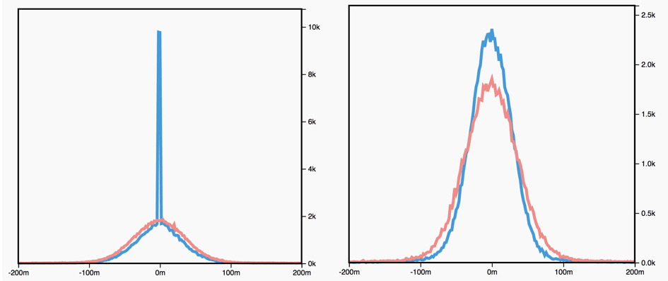
- The figure below shows a histogram of weight values for an unregularized (red) and \(L_1\) regularized (blue left) and \(L_2\) regularized (blue right) network:
-
The different effects of \(L_1\) and \(L_2\) regularization on the optimal parameters are an artifact of the different ways in which they change the original loss landscape. In the case of two parameters (\(w_1\) and \(w_2\)), we can visualize this.
-
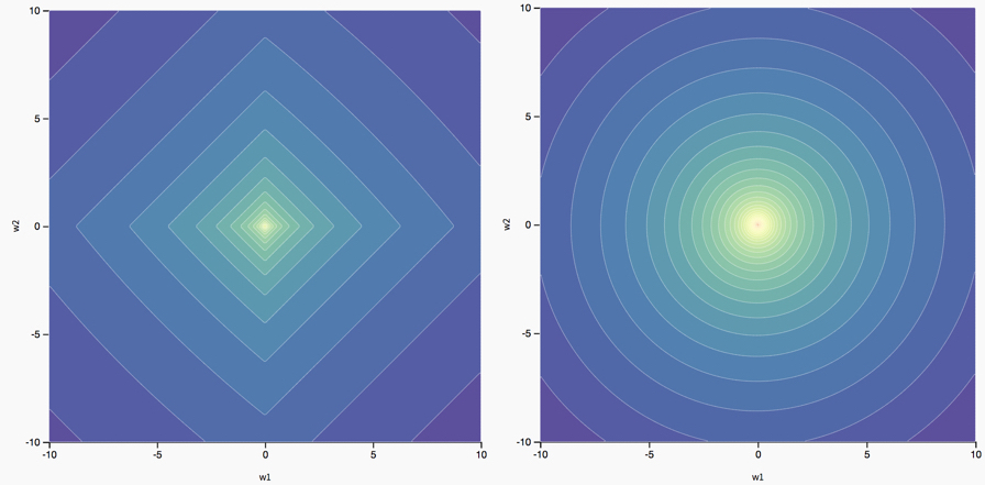
The figure below shows the landscape of a two parameter loss function with \(L_1\) regularization (left) and \(L_2\) regularization (right):
\(L_1\) vs. \(L_2\) regularization
-
\(L_2\) and \(L_1\) penalize weights differently:
- \(L_2\) penalizes \(weight^2\).
- \(L_1\) penalizes \(\|weight\|\).
-
Consequently, \(L_2\) and \(L_1\) have different derivatives:
- The derivative of \(L_2\) is \(2 * weight\).
- The derivative of \(L_1\) is \(k\) (a constant, whose value is independent of the weight but depends on the sign of the weight).
- You can think of the derivative of \(L_2\) as a force that removes \(x\%\) of the weight every time. As Zeno knew, even if you remove \(x\%\) of a number billions of times, the diminished number will still never quite reach zero. (Zeno was less familiar with floating-point precision limitations, which could possibly produce exactly zero.) At any rate, \(L_2\) does not normally drive weights to zero.
- Simply put, for \(L_2\), the smaller the \(w\), the smaller the penalty during the update of \(w\) and vice-versa for larger \(w\).
\(L_2\) regularization results in a uniform distribution of weights, as much as possible, over the entire weight matrix.
- You can think of the derivative of \(L_1\) as a force that subtracts some constant from the weight every time, irrespective of the weight’s magnitude. However, thanks to absolute values, \(L_1\) has a discontinuity at 0, which causes subtraction results that cross 0 to become zeroed out. For example, if subtraction would have forced a weight from +0.1 to -0.2, \(L_1\) will set the weight to exactly 0. Eureka, \(L_1\) zeroed out the weight!
- Simply put, for \(L_1\), note that while the penalty is independent of the value of \(w\), but the direction of the penalty (positive or negative) depends on the sign of \(w\).
\(L_1\) regularization thus results in an effect called “feature selection” or “weight sparsity” since it makes the irrelevant weights 0.
-
\(L_1\) regularization – penalizing the absolute value of all the weights – turns out to be quite efficient for wide models.
- Note that this description is true for a one-dimensional model.
Effect of \(L_1\) and \(L_2\) regularization on weights
-
Both \(L_1\) and \(L_2\) regularization have a dramatic effect on the weights values during training.
- For \(L_1\) regularization:
- “Too small” \(\lambda\) constant: there’s no apparent effect.
- “Appropriate” \(\lambda\) constant: many of the weights become zeros. This is called “sparsity of the weights”. Because the weight penalty is independent of the weight values, weights with value 0.001 are penalized just as much as weights with value 1000. The value of the penalty is \(\alpha \lambda\) (generally very small). It constrains the subset of weights that are “less useful to the model” to be equal to 0. For example, you could effectively end up with 200 non-zero weights out of 1000, which means that 800 weights were less useful for learning the task.
- “Too large” \(\lambda\) constant: You can observe a plateau, which means that the weights uniformly take values around zero. In fact, because \(\lambda\) is large, the penalty −\(\alpha \lambda sign(w)\) is much higher than the gradient −\(\alpha \frac{\partial J_{cross−entropy}}{\partial w}\). Thus, at every update, \(w\) is pushed by \(\approx −\alpha\lambda sign(w)\) in the opposite direction of its sign. For instance, if w is around zero, but slightly positive, then it will be pushed towards −\(\alpha \lambda\) when the penalty is applied. Hence, the plateau’s width should be \(2 \times \alpha \lambda\).
- For \(L_2\) regularization:
- “Too small” \(\lambda\) constant: there’s no apparent effect.
- “Appropriate” \(\lambda\) constant: the weight values decrease following a centered distribution that becomes more and more peaked throughout training.
- “Too large” \(\lambda\) constant: All the weights are rapidly collapsing to zeros, and the model obviously underfits because the weight values are too constrained.
- Note that the weight sparsity effect caused by \(L_1\) regularization makes your model more compact in theory, and leads to storage-efficient compact models that are commonly used in smart mobile devices.
Choosing \(L_1\)-norm vs. \(L_2\)-norm as the regularizing function
-
In a typical setting, the \(L_2\)-norm is better at minimizing the prediction error over the \(L_1\)-norm. However, we do find the \(L_1\)-norm being used despite the \(L_2\)-norm outperforming it in almost every task, and this is primarily because the \(L_1\)-norm is capable of producing a sparser solution.
-
To understand why an \(L_1\)-norm produces sparser solutions over an \(L_2\)-norm during regularization, we just need to visualize the spaces for both the \(L_1\)-norm and \(L_2\)-norm as shown in the figure below (source).

-
In the diagram above, we can see that the solution for the \(L_1\)-norm (to get to the line from inside our diamond-shaped space), it’s best to maximize \(x_1\) and leave \(x_2\) at 0, whereas the solution for the \(L_2\)-norm (to get to the line from inside our circular-shaped space), is a combination of both \(x_1\) and \(x_2\). It is likely that the fit for \(L_2\) will be more precise. However, with the \(L_1\) norm, our solution will be more sparse.
-
Since the \(L_2\)-norm penalizes larger errors more strongly, it will yield a solution which has fewer large residual values along with fewer very small residuals as well.
-
The \(L_1\)-norm, on the other hand, will give a solution with more large residuals, however, it will also have a lot of zeros in the solution. Hence, we might want to use the \(L_1\)-norm when we have constraints on feature extraction. We can easily avoid computing a lot of computationally expensive features at the cost of some of the accuracy, since the \(L_1\)-norm will give us a solution which has the weights for a large set of features set to 0. A use-case of \(L_1\) would be real-time detection or tracking of an object/face/material using a set of diverse handcrafted features with a large margin classifier like an SVM in a sliding window fashion, where you would probably want feature computation to be as fast as possible in this case.
-
Another way to interpret this is that \(L_2\)-norm basically views all features similarly since it assumes all the features to be “equidistant” (given its geometric representation as a circle), while \(L_1\) norm views different features differently since it treats the “distance” between them differently (given its geometric representation as a square). Thus, if you are unsure of the kind of features available in your dataset and their relative importance, \(L_2\) regularization is the way to go. On the other hand, if you know that one feature matters much more than another, use \(L_1\) regularization.
-
In summary,
- Broadly speaking, \(L_1\) is more useful for “what?” and \(L_2\) is more “how much?”.
- The \(L_1\) norm isn’t smooth, which is less about ignoring fine detail and more about generating sparse feature vectors. Sparse is sometimes good e.g., in high dimensional classification problems.
- The \(L_2\) norm is as smooth as your floats are precise. It captures energy and Euclidean distance, things you want when, for e.g., tracking features. It’s also computation heavy compared to the \(L_1\) norm.
How does adding a penalty term/component to the loss term prevent overfitting with regularization?
- Adding a penalty term/component to the loss term for \(L_1\) (Lasso) and \(L_2\) (Ridge) regularization helps prevent overfitting by penalizing overly complex models, encouraging simpler ones that generalize better to unseen data. The penalty term in the loss function penalizes large weights, which
. By controlling model complexity, regularization encourages the model to focus on generalizable patterns rather than specific data points, making it less sensitive to the idiosyncrasies of the training data. -
Here’s how this works in detail:
- Penalizing Large Weights:
In models like neural networks or linear regressions, overfitting often involves assigning high weights to certain features, which makes the model sensitive to noise in the training data.
- Regularization adds a term to the loss function (e.g., \(\lambda \sum_{i} w_i^2\) for \(L_2\) regularization) that penalizes large weights. By keeping weights smaller, the model learns a smoother mapping that’s less likely to fit noise.
-
Balancing Fit with Complexity: The regularization term adds a trade-off in the loss function between fitting the training data well and keeping the model complexity in check. For instance, with a regularized loss function \(\text{Loss} = \text{MSE} + \lambda \sum_{i} w_i^2\), the regularization strength \(\lambda\) controls how much weight is given to reducing error versus limiting model complexity. A well-chosen \(\lambda\) helps the model to capture only the significant patterns, not the noise.
-
Improved Generalization: By limiting the capacity of the model to learn very specific mappings, regularization helps the model to generalize better to new data. Overly flexible models tend to memorize training examples, while regularized models are forced to learn broader trends, which results in better performance on validation or test datasets.
- Types of Regularization Penalties:
- \(L_1\) Regularization (Lasso): Adds an absolute penalty (e.g., \(\lambda \sum_{i} \|w_i\|\)), encouraging sparse models by pushing some weights to zero. This can also perform feature selection by removing less useful features.
- \(L_2\) Regularization (Ridge): Penalizes the square of the weights, encouraging the model to spread weight values across many parameters rather than making any one parameter large. This results in smoother models.
- Penalizing Large Weights:
FAQ: Why does \(L_1\) regularization lead to feature selection or weight sparsity while \(L_2\) results in weight decay/shrinkage (i.e., uniform distribution of weights)?
- \(L_1\) and \(L_2\) regularization affect the weights of features differently, leading to distinct outcomes: feature selection in the case of \(L_1\) and uniform weight shrinkage in the case of \(L_2\). These differences arise from the mathematical and geometric properties of their respective penalty functions.
- These distinctions can serve as a guideline to choose the appropriate regularization method based on the problem requirements, such as whether feature selection or weight smoothness is more important.
\(L_1\) Regularization: Feature Selection and Weight Sparsity
-
Penalty: The penalty term added to the loss function is proportional to the absolute value of the weights:
\[\lambda \sum |w_i|\] -
Effect on Weights: The absolute value function is non-differentiable at zero, creating a “sharp corner” in the optimization landscape. This sharpness allows gradient-based optimization methods (e.g., gradient descent) to drive some weights exactly to zero.
-
Geometric Interpretation: \(L_1\) regularization constrains the optimization problem within a diamond-shaped polytope (or more generally, an \(L_1\)-norm ball). The sharp vertices of this polytope align with the coordinate axes, making it more likely for the optimization process to find solutions where weights for some features are exactly zero. This sparsity is a natural consequence of the sharp corners in the constraint surface.
-
Feature Selection: By driving irrelevant or redundant feature weights to zero, \(L_1\) regularization effectively removes these features from the model. This makes \(L_1\) particularly useful in situations where feature selection is critical, such as high-dimensional datasets with many irrelevant or noisy features.
\(L_2\) Regularization: Weight Shrinkage (i.e., Uniform Distribution of Weights)
-
Penalty: The penalty term added to the loss function is proportional to the square of the weights:
\[\lambda \sum w_i^2\] -
Effect on Weights: The squared function is smooth and differentiable everywhere, including at zero. During optimization, this smoothness results in a uniform force that shrinks all weights toward zero. However, unlike \(L_1\), it does not eliminate any weight entirely.
-
Geometric Interpretation: \(L_2\) regularization constrains the optimization problem within a spherical region (or more generally, an \(L_2\)-norm ball) – specifically, a hypersphere (or ellipse in lower dimensions). The smooth, curved surface of the sphere distributes the penalty evenly across all dimensions. The smooth curve distributes the penalty such that larger weights are penalized more heavily than smaller weights, encouraging the model to learn more balanced and generalized patterns. In other words, this even distribution ensures that all weights are reduced proportionally to their magnitude, rather than being selectively driven to zero.
-
Weight Shrinkage: The uniform shrinkage helps the model generalize better by reducing the influence of less important features while retaining all features in the model. This makes \(L_2\) regularization particularly effective when all features contribute meaningfully to the prediction, even if some are less significant than others.
Key Differences Between \(L_1\) and \(L_2\)
Mathematical Properties
- Penalty Function:
-
\(L_1\): Proportional to the absolute value of the weights ($$ w_i $$). - \(L_2\): Proportional to the square of the weights (\(w_i^2\)).
-
- Behavior Around Zero:
- \(L_1\): Sharp corners in the absolute value function create a discontinuity in its derivative at zero, favoring sparsity by driving weights exactly to zero.
- \(L_2\): The squared function is smooth and differentiable everywhere, resulting in gradual weight reduction without setting weights to zero.
Geometric Interpretation
- \(L_1\): The diamond-shaped constraint region (from the \(L_1\)-norm ball) promotes sparse solutions by aligning weights with the coordinate axes, naturally driving some weights to zero.
-
\(L_2\): The spherical constraint region (from the \(L_2\)-norm ball) distributes the penalty evenly across all dimensions, resulting in proportional weight reduction and smoother, more uniform weight distributions.
- Both methods mitigate overfitting but suit different needs: \(L_1\) for sparse models and feature selection, and \(L_2\) for smoother, more distributed weight adjustments.
Dropout Regularization
- Although \(L_1\) and \(L_2\) regularization are simple techniques to reducing overfitting, there exist other methods, such as dropout regularization, that have been shown to be more effective at regularizing larger and more complex networks. If you had unlimited computational power, you could improve generalization by averaging the predictions of several different neural networks trained on the same task. The combination of these models will likely perform better than a single neural network trained on this task. However, with deep neural networks, training various architectures is expensive because:
- Tuning the hyperparameters is time consuming.
- Training the networks requires a lot of computations.
- You need a large amount of data to train the models on different subsets of the data.
- Dropout is a regularization technique, introduced in Srivastava et al. (2014), that allows you to combine many different architectures efficiently by randomly dropping some of the neurons of your network during training.
- For more details, please refer to the Dropout primer.
Label Smoothing
- Similar to L1/L2 Regularization and Dropout Regularization, Label smoothing is a regularization technique used in training machine learning models, particularly in classification tasks, to enhance generalization and model robustness. Instead of using hard, one-hot encoded targets during training, label smoothing redistributes a small portion of the probability mass from the correct class to other classes. This adjustment prevents the model from becoming overly confident in its predictions and reduces the risk of overfitting.
- By introducing this slight uncertainty, label smoothing improves the reliability and robustness of classification models, making them better equipped to handle real-world applications. Its simplicity and effectiveness make it a powerful tool for creating models that generalize well across diverse datasets.
Why Use Label Smoothing?
- Avoid Overconfidence:
- Without label smoothing, models are trained to output a probability of
1for the correct class and0for all others. This can lead to overconfident predictions, where the model assigns very high probabilities to a single class. - Overconfidence can harm generalization and make the model less robust to adversarial attacks or noisy data.
- Without label smoothing, models are trained to output a probability of
- Reduce Overfitting:
- Hard labels can lead to the model memorizing the training data. Label smoothing acts as a form of regularization by making the model less likely to overfit.
- Encourage Calibration:
- Label smoothing ensures that the predicted probabilities better reflect the true likelihood of an event, improving the model’s calibration.
How Label Smoothing Works
- Let:
- \(y\) be the one-hot encoded target vector for a sample.
- \(\hat{y}\) be the predicted probability distribution from the model.
- \(\epsilon\) be the label smoothing parameter (usually a small value like 0.1).
-
The smoothed target distribution \(y'\) is computed as:
\(y'_i = (1 - \epsilon) \cdot y_i + \frac{\epsilon}{N}\)
- where:
- \(N\) is the number of classes.
- \(y_i\) is the original target probability (1 for the correct class, 0 for others).
- where:
- This equation redistributes the probability mass:
- The correct class has a slightly lower probability \(1 - \epsilon + \frac{\epsilon}{N}\).
- All other classes are assigned a small non-zero probability \(\frac{\epsilon}{N}\).
- For example, if \(\epsilon = 0.1\) and \(N = 3\) (three classes), the original one-hot label [1, 0, 0] becomes:
Loss Function with Label Smoothing
- Label smoothing is typically applied to the cross-entropy loss function. The smoothed target distribution \(y'\) is used instead of the one-hot labels:
- This modifies the loss function to penalize extreme predictions and prevents the model from being overly confident.
Benefits of Label Smoothing
- Improved Generalization:
- Models trained with label smoothing tend to perform better on unseen data.
- Prevention of Overconfidence:
- Reduces the tendency of the model to assign overly high probabilities to a single class.
- Better Handling of Noisy Labels:
- Smoothing the labels helps mitigate the effect of mislabeled data by distributing the probability mass.
- Enhanced Calibration:
- Predictions are more probabilistically sound and calibrated.
When to Use Label Smoothing
- Label smoothing is most beneficial in:
- Classification tasks with a large number of classes (e.g., ImageNet, language modeling).
- Scenarios where the labels might be noisy or uncertain.
- Models prone to overfitting, such as deep neural networks.
- Avoid label smoothing in:
- Applications where hard decisions are necessary, such as problems involving imbalanced classes or where probabilities must reflect sharp distinctions.
Practical Considerations
- Choosing \(\epsilon\):
- Common values for \(\epsilon\) range from 0.05 to 0.2. Experimentation is often necessary to find the best value.
- Implementation:
- Most deep learning frameworks (e.g., TensorFlow, PyTorch) support label smoothing either directly or through custom loss functions.
References
- Machine Learning Crash Course by Google: Regularization
- When would you choose \(L_1\)-norm over \(L_2\)-norm?
Further Reading
- A Simple Weight Decay Can Improve Generalization
- The Bayesian interpretation of weight decay
- Dropout: A Simple Way to Prevent Neural Networks from Overfitting
- Learning Compact Neural Networks with Regularization
- \(L_0\) Norm, \(L_1\) Norm, \(L_2\) Norm & L-Infinity Norm
Citation
If you found our work useful, please cite it as:
@article{Chadha2020DistilledRegularization,
  title   = {Regularization},
  author  = {Chadha, Aman},
  journal = {Distilled AI},
  year    = {2020},
  note    = {\url{https://aman.ai}}
}