Primers • Recursive Transformers
- Overview
- Looped Transformers
- Overview
- Why Recurrent Depth Instead of Unique Depth?
- Parameters, effective depth, and compute
- The parameter-sharing cost
- Why recurrence can still be attractive
- Recurrence must usually be trained as recurrence
- More loops are not necessarily better
- Adaptive depth and token-level computation
- KV-cache memory is a separate problem
- Recurrent depth and chain-of-thought monitorability
- Practical interpretation
- Research Lineage
- Core Mechanism
- Why It Matters
- Latent Reasoning
- Iterative Computation
- Knowledge Use
- Why Recurrent Depth Instead of Unique Depth?
- Architecture
- Training
- Stability
- Scaling Laws
- Reasoning
- Chain-of-Thought Monitorability
- Architecture and monitorability are different properties
- Why recurrent depth changes the monitorability question
- What chain-of-thought monitorability measures
- Longer reasoning traces can improve monitorability
- Chain-of-thought monitorability is not the same as faithfulness
- Latent reasoning need not be uninterpretable by construction
- Recurrent depth does not by itself explain current monitorability regressions
- How to test whether recurrence causes a monitorability loss
- Monitoring beyond natural-language reasoning
- Takeaway
- Generalization
- Test-Time Compute
- Universal Transformers: Recurrent Self-Attention over Depth
- Staircase and Ladder Attention
- Implementations
- Open Questions
- Claude Mythos Speculation
- Overview
- Recursive Latent Reasoning
- Recursive Language Models
- References
- Citation
Overview
-
Recursive transformers are best understood as transformer architectures that reuse computation across depth rather than assigning a fresh set of parameters to every layer in a deep stack. The broad motivation is simple: many tasks may require more iterative computation without necessarily requiring a proportionally larger number of stored weights.
-
The central idea is recurrence over computation. A recursive transformer can apply the same block, or a small stack of blocks, multiple times to refine hidden states. This makes effective depth partly a runtime choice: the model can spend more computation by looping, while keeping parameter count relatively compact.
-
This framing gives three related but distinct paradigms:
-
Looped transformers: These are the core recursive transformer family. They reuse shared transformer blocks across depth, increasing effective depth through repeated latent refinement. Universal Transformers by Dehghani et al. (2018) introduced an early recurrent self-attentive architecture with shared transition functions and adaptive computation, while Looped Transformers Are Better at Learning Learning Algorithms by Yang et al. (2024) showed that looped transformers can emulate iterative learning algorithms with far fewer parameters than standard transformers.
-
Recursive latent reasoning models: These extend the same “reuse computation” intuition beyond standard transformer depth. Instead of merely looping layers, they repeatedly update hidden reasoning states. Training Large Language Models to Reason in a Continuous Latent Space by Hao et al. (2024) introduced Coconut, where continuous hidden states are fed back as reasoning states instead of decoding every reasoning step into words; Hierarchical Reasoning Model by Wang et al. (2025) and Less is More: Recursive Reasoning with Tiny Networks by Jolicoeur-Martineau (2025) apply recursive latent refinement to compact supervised reasoning networks.
-
Recursive Language Models: These are not recursive transformers in the architectural sense, but they are important to contrast with them. RLMs move recursion outside the neural network: a standard model can be wrapped in an inference scaffold that stores long context externally, lets the model inspect it programmatically, and recursively calls models on selected subcontexts. Recursive Language Models by Zhang et al. (2025) introduced RLMs as a systems-level inference strategy for long-context control and recursive task decomposition.
-
-
The key takeaway is that recursive transformers mainly address reasoning depth, while RLMs mainly address context control. Looped transformers, HRM, TRM, Coconut, and recurrent-depth models try to make a model think more deeply before answering. RLMs try to make a model control a computation over context that is too large, dense, or structured to read directly.
Recursive model families at a glance
-
Looped transformers scale neural networks by reusing the same transformer block, or a small stack of blocks, multiple times during a single forward pass. Instead of assigning a distinct set of parameters to every layer in a deep stack, a looped model repeatedly applies shared parameters to refine the hidden state. This increases effective depth while keeping parameter count fixed, making compute a runtime resource rather than only a static architectural choice. Scaling up Test-Time Compute with Latent Reasoning: A Recurrent Depth Approach by Geiping et al. (2025) shows that a language model can scale test-time compute by repeatedly applying a recurrent block in latent space rather than producing more chain-of-thought tokens. ([GitHub][4])
-
The core promise of looped transformers is straightforward: a compact model can spend more computation on difficult inputs while keeping stored weights relatively small. They reuse weights across depth, increase computation through recurrence, and perform iterative latent refinement before producing output. This makes compute a runtime knob: increasing loop count can increase effective reasoning depth without proportionally increasing parameter count.
-
HRM and TRM are recursive latent reasoning models that recurse inside compact reasoning networks rather than inside large language-model prompts. Hierarchical Reasoning Model by Wang et al. (2025) uses two interdependent recurrent modules operating at different timescales, while Less is More: Recursive Reasoning with Tiny Networks by Jolicoeur-Martineau (2025) simplifies this into a single tiny recursive network that improves the answer over repeated latent steps.
-
RLMs recurse outside the neural network. Recursive Language Models by Zhang et al. (2025) turns the long prompt into an external environment object and lets the model programmatically inspect, decompose, and recursively call itself over selected snippets.
-
A useful summary is:
| Family | Where recursion happens | What is reused | Main goal |
|---|---|---|---|
| Looped transformers | Transformer depth | Shared layer blocks | More latent reasoning per token |
| HRM | Two latent recurrent modules | High-level and low-level recurrent states | Puzzle solving through hierarchical latent refinement |
| TRM | One tiny recursive network | A single latent reasoning state | Simpler recursive refinement with fewer parameters |
| RLMs | Inference scaffold | Model calls, REPL state, child calls | Long-context control and recursive task decomposition |
Three kinds of recursion
-
The first kind is architectural recursion. A looped transformer repeatedly applies the same block to hidden states, increasing effective depth without adding a proportional number of parameters. The core motivation is that many reasoning and algorithmic tasks require substantial depth, but not necessarily a proportional increase in unique parameters. A model may need to think longer rather than know more. Reasoning with Latent Thoughts: On the Power of Looped Transformers by Saunshi et al. (2025) argues that many reasoning problems require large depth but not necessarily many parameters, and demonstrates that a \(k\)-layer transformer block looped \(L\) times can behave similarly to a \(kL\)-layer transformer on reasoning tasks.
-
The second kind is latent state recursion. HRM and TRM do not mainly target language modeling or long-context reading. They target compact, supervised reasoning over hard puzzle-like tasks. HRM separates slow abstract planning from fast detailed computation, while TRM removes the hierarchy and recurses one small network over its latent reasoning feature. Less is More: Recursive Reasoning with Tiny Networks by Jolicoeur-Martineau (2025) reports that TRM reduces the architecture to a single tiny network while outperforming HRM on several puzzle benchmarks.
-
The third kind is systems recursion. RLMs do not require changing the transformer architecture. A standard model can be wrapped in a REPL-style environment, where the full context is stored as a variable and the model writes code to inspect it. This means recursion appears as a trajectory of actions, observations, and subcalls rather than as hidden-state recurrence. Recursive Language Models describes this design as replacing the usual completion call with an RLM call that offloads context into a REPL environment.
Context vs. reasoning
-
Looped transformers, HRM, and TRM primarily attack reasoning depth. They ask whether a model can spend more computation before committing to an answer.
-
Looped transformers answer this question by making effective depth variable. A conventional deep transformer usually pays for depth with more unique layers. A looped transformer instead sends activations through the same block repeatedly, so the same parameters can implement multiple rounds of latent refinement. Looped Transformers Are Better at Learning Learning Algorithms by Yang et al. (2024) shows that looped transformers can solve in-context data-fitting problems with performance comparable to standard transformers while using far fewer parameters, which supports the view that recurrence can help emulate iterative algorithms.
-
RLMs primarily attack context control. They ask whether a model can avoid reading the entire context directly and instead choose which parts to inspect, delegate, and aggregate.
-
This distinction matters. A looped transformer may reason more deeply within its context window, but it still needs the relevant input to be present in that window. An RLM can work when the relevant input is not initially inside the model window, because the full prompt is stored externally and accessed through code, search, slicing, and recursive calls. Recursive Language Models by Zhang et al. (2025) reports that RLMs handle inputs up to two orders of magnitude beyond model context windows while remaining competitive in query cost.
Latent vs. explicit work
-
Recursive latent reasoning keeps intermediate computation hidden. In a looped transformer, HRM, or TRM, the useful intermediate state is a vector. The model may refine an internal solution repeatedly, but there is no natural human-readable trace unless one is added externally.
-
This latent form of extra computation is the main attraction of looped transformers. They can “think” by updating hidden states rather than by emitting more text. Scaling Latent Reasoning via Looped Language Models by Zhu et al. (2025) presents Ouro, a family of looped language models that build reasoning into pretraining through iterative latent computation, learned depth allocation, and large-scale training.
-
RLMs expose intermediate work as an execution trace. The root model can search, print snippets, store variables, call children, aggregate outputs, and return a final variable. This makes RLMs more auditable and easier to debug, but also more dependent on scaffolding quality, sandboxing, prompts, and runtime budgets.
-
This gives the two paradigms different engineering profiles:
| Dimension | Recursive latent reasoning | Recursive Language Models |
|---|---|---|
| Intermediate state | Hidden vectors | REPL variables and action history |
| Main output mode | Direct prediction | Final answer or environment variable |
| Debuggability | Low unless instrumented | High through trajectory logs |
| Training style | Architecture-specific supervised or generative training | Prompting, SFT, RL over trajectories |
| Failure mode | Bad latent iteration, overthinking, poor generalization | Bad decomposition, over-recursion, observation flooding |
- Training Large Language Models to Reason in a Continuous Latent Space by Hao et al. (2024) motivates latent-space reasoning by arguing that natural language is not always the best substrate for thought, while RLMs take the opposite systems tradeoff by making reasoning steps explicit through tool-mediated environment interaction.
HRM and TRM
-
HRM is a compact recurrent architecture for supervised reasoning. Its high-level module performs slower abstract planning, and its low-level module performs faster detailed computation. The model executes a sequence of latent reasoning updates in a single forward pass without explicit supervision of the intermediate reasoning trace. Hierarchical Reasoning Model by Wang et al. (2025) reports strong results on Sudoku-Extreme, Maze-Hard, and ARC-AGI using about 27M parameters and around 1000 training examples.
-
TRM simplifies HRM by removing the two-network hierarchy. Instead of separate high-frequency and low-frequency modules, it uses a single tiny network that recursively refines a latent reasoning feature and progressively improves the answer. Less is More: Recursive Reasoning with Tiny Networks by Jolicoeur-Martineau (2025) reports TRM-Att at 7M parameters reaching 44.6% on ARC-AGI-1 and 7.8% on ARC-AGI-2, compared with HRM’s 40.3% and 5.0% in the same reported table.
-
The key lesson from HRM and TRM is that recursion can be useful even without language, tools, or chain-of-thought. These models suggest that some reasoning problems benefit from repeated latent refinement rather than more text generation or larger pretrained models.
RLMs as outer recursion
-
RLMs are the outer-loop counterpart to latent recursive reasoning. Instead of asking a neural block to refine hidden states, an RLM asks a language model to refine a computation over an external context. The root model can inspect structure, form hypotheses, call child models on subproblems, and assemble a final result.
-
A minimal RLM trajectory looks like this:
context = load_context()
history = []

for step in range(max_steps):
    action = root_model(query, history)
    observation = repl.execute(action)
    history.append((action, observation))

    if is_final(action):
        return resolve_final(action)
- The core computation is:
- This differs from HRM and TRM because the recursive state is not only a vector. It can be a Python variable, a list of candidate documents, a dictionary of evidence spans, a cache of child outputs, or a partially constructed report. alexzhang13/rlm describes this as a plug-and-play inference library that offloads context as a REPL variable and exposes sub-LM calls inside the environment.
Training link
-
The training story connects the two worlds. HRM and TRM are trained to perform recursive latent refinement directly. RLMs can initially be prompted, but the stronger path is to train the model as a recursive control policy.
-
Reinforcing Recursive Language Models by Kim and Ahmad (2026) trains small 4B models to behave as native RLMs by using one shared policy for both parent and child roles, so the model learns when to decompose, when to call children, and when to stop.
-
This makes RLM training structurally similar to latent recursive reasoning, but at a different level. HRM and TRM train the recurrent update rule inside the network. Reinforced RLMs train the action policy outside the network:
| Training target | HRM / TRM | RLM |
|---|---|---|
| Learned recurrence | Latent state update | External action sequence |
| Action-selection policy | Implicit in recurrent dynamics | Explicit tool, search, child-call, and finalization choices |
| Intermediate signal | Supervised answer refinement | Trajectory reward and child-call outcomes |
| Reused computation | Tiny recurrent module | Root and child model calls |
| Main skill | Internal iterative reasoning | External context decomposition |
- Looped transformers add a third training pattern: the model must learn to make repeated applications of shared weights useful rather than unstable or redundant. Parcae: Scaling Laws For Stable Looped Language Models by Prairie et al. (2026) studies looped architectures as dynamical systems and focuses on stabilizing recurrence so that increasing loops can improve quality rather than causing residual explosion or loss spikes.
Combined path
-
The cleanest way to connect the dots is to see recursive latent reasoning and RLMs as complementary layers of test-time computation.
-
A looped transformer, HRM-like model, or TRM-like model can make each model call better by spending more latent compute. An RLM can make the whole task better by deciding which calls to make and what context each call should see.
-
A future system could combine both:
root_model = latent_recursive_model()
child_model = latent_recursive_model()

rlm = RLM(
    root_model=root_model,
    child_model=child_model,
    environment=PythonREPL(),
    max_child_calls=64,
)
-
In that hybrid, recursion happens twice: internally through latent refinement and externally through environment-mediated decomposition. The latent model improves local reasoning; the RLM scaffold improves global context control.
-
Looped transformers make this hybrid especially natural because they separate stored parameters from runtime compute. A child model inside an RLM could spend only a few loops on easy snippets and more loops on hard snippets, while the parent RLM decides which snippets deserve child calls at all. This gives two independent control knobs: latent compute per call and recursive decomposition across calls.
Looped Transformers
Overview
Why Recurrent Depth Instead of Unique Depth?
Parameters, effective depth, and compute
- The central trade-off in recurrent-depth transformers is that parameter count and computational depth become separate quantities. Suppose a model contains parameters used only once, \(N_{\text{once}}\), and a recurrent block containing \(N_{\text{rec}}\) parameters that is executed \(r\) times. The number of distinct stored parameters is:
- However, the amount of parameterized computation executed during a forward pass scales approximately as:
-
Consequently, recurrent depth does not automatically make a model computationally cheaper than a conventional transformer with the same effective depth. It primarily makes the model smaller in terms of distinct weights. How Much Is One Recurrence Worth? Iso-Depth Scaling Laws for Looped Language Models by Schwethelm et al. (2026) formalizes this distinction by constructing looped and non-looped models with matched effective depth and nearly matched FLOPs while varying the number of unique parameters.
-
Ignoring smaller attention and embedding corrections, the forward-pass FLOPs of such a recurrent model can be approximated as:
-
If a \(k\)-layer stack is reused \(r\) times, its effective depth is \(D_{\text{eff}}=kr\) but its stored layer parameters correspond to only \(k\) distinct layers. A \(22\)-layer stack executed twice therefore performs \(44\) layer applications while storing only \(22\) unique layer parameter sets.
-
Nanbeige4.2-3B: Unlocking Agentic Capabilities in a Compact Model by Nanbeige Lab et al. (2026) provides a concrete large-scale example: its hidden states pass through the same Transformer stack for a second pass, increasing computational depth without introducing a second set of layer parameters. The model is pretrained from scratch on \(28\) trillion tokens with this recurrent structure.
The parameter-sharing cost
-
Reusing a block is not generally equivalent to replacing every recurrence with a fresh set of parameters. Unique layers can learn specialized transformations for different depths, whereas a recurrent block must implement a reusable update rule that remains useful every time it is applied.
-
How Much Is One Recurrence Worth? Iso-Depth Scaling Laws for Looped Language Models by Schwethelm et al. (2026) quantifies this loss of expressivity through a recurrence-equivalence exponent \(\varphi\). The effective parameter capacity of a recurrent model is modeled as:
-
This produces the joint scaling law:
\[\mathcal{L} = E + A \left( N_{\text{once}} + r^{\varphi}N_{\text{rec}} \right)^{-\alpha} + BD^{-\beta}\]- where \(D\) is the number of training tokens, \(E\) is irreducible loss, and \(\alpha\) and \(\beta\) describe parameter and data scaling respectively.
-
The exponent has a useful interpretation:
- \(\varphi=0\) means executing the shared block repeatedly adds essentially no parameter-equivalent capacity.
- \(\varphi=1\) means each recurrence is as useful as introducing an equivalent fresh block of parameters.
- \(0<\varphi<1\) means recurrence adds useful computation, but less capacity than an equally expensive stack of unique layers.
-
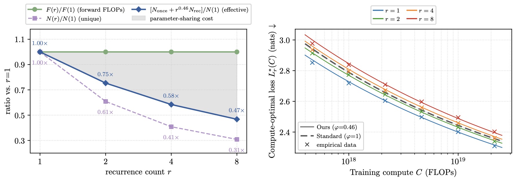
Across \(116\) iso-depth pretraining runs with \(r\in\{1,2,4,8\}\), Schwethelm et al. estimate \(\varphi \approx 0.46\) for their baseline recurrent architecture. At \(r=4\), for example, a \(410\)M-parameter looped model matched the loss of an approximately \(580\)M-parameter non-looped model while paying training compute comparable to a roughly \(1\)B-parameter non-looped model. This provides a quantitative expression of the parameter-sharing tax: additional recurrence is useful, but a recurrent pass is not generally worth an entire fresh block of weights.
-
The following figure (source) shows the recurrence-equivalence trade-off: at matched effective depth, forward FLOPs remain approximately constant while unique parameter count falls with increasing recurrence, and the fitted \(\varphi=0.46\) scaling law places the effective capacity of looped models between the extremes of no recurrence benefit and full equivalence to unique layers.
Why recurrence can still be attractive
-
The existence of a parameter-sharing cost does not imply that recurrent depth is undesirable. It means that recurrence and ordinary depth optimize different resource constraints.
-
First, recurrent models can be attractive when parameter memory is more restrictive than FLOPs. A model that repeatedly executes a smaller set of weights can achieve substantially greater effective depth without loading the weights of an equivalently deep non-looped architecture. This matters when the alternative would require additional devices, additional parameter sharding, or substantially more memory bandwidth.
-
Second, recurrence introduces an iterative inductive bias. The same learned operator repeatedly transforms an evolving state:
which naturally resembles iterative optimization, search, constraint propagation, or numerical algorithms. Looped Transformers are Better at Learning Learning Algorithms by Yang et al. (2024) showed that looped transformers can learn iterative data-fitting procedures while using less than 10% of the parameters of comparable standard transformers.
-
Third, recurrent depth exposes computation as an inference-time control variable. Scaling up Test-Time Compute with Latent Reasoning: A Recurrent Depth Approach by Geiping et al. (2025) trains a recurrent-depth language model whose shared block can be unrolled further at inference time; its 3.5B-parameter model continued obtaining reasoning improvements at computational loads corresponding to much larger conventional models.
-
Fourth, newer architectures can reduce the parameter-sharing penalty itself. Loop the Loopies! by Gao et al. (2026) explicitly begins from the observation that naively spending an \(N\)-fold larger pretraining budget on \(N\) recurrences has historically been weaker than spending that budget on \(N\) times more parameters, but reports that its Loopie MoE architectures can outperform compute-matched vanilla Transformer baselines.
Recurrence must usually be trained as recurrence
-
Simply taking a pretrained conventional transformer and executing its layers twice is not equivalent to training a recurrent model. A standard transformer has been optimized under the assumption that each layer processes the distribution of states produced by its unique predecessor. Reapplying a block changes this state distribution.
-
Nanbeige4.2-3B: Unlocking Agentic Capabilities in a Compact Model by Nanbeige Lab et al. (2026) directly compared upcycling a standard transformer into a looped architecture with pretraining the recurrent architecture from scratch. The from-scratch model performed substantially better, suggesting that representations learn to adapt to repeated parameter reuse throughout training.
-
This result should not be interpreted as proving that retrofitting is impossible. Instead, naive recurrence is usually unstable because the reused block receives states it was never trained to process. Training-Free Looped Transformers by Chen et al. (2026) shows that straightforward block reapplication generally degrades performance, but develops a training-free method that interprets pretrained residual blocks as numerical integration steps and replaces a large update with smaller damped recurrent substeps. The resulting method improves several frozen dense and MoE checkpoints without additional finetuning.
-
Thus, there are two distinct approaches:
- Native recurrence trains the network from the beginning to treat its shared block as an iterative update operator.
- Retrofitted recurrence modifies how a pretrained operator is reapplied so that repeated passes remain close to its original learned dynamics.
More loops are not necessarily better
-
Increasing recurrent depth is useful only while successive passes continue making productive changes to the representation. Beyond that point, additional loops can produce diminishing returns, instability, or even regressions.
-
In Nanbeige4.2-3B: Unlocking Agentic Capabilities in a Compact Model by Nanbeige Lab et al. (2026), two passes were selected as the best empirical trade-off. The two-pass configuration retained approximately 75% of the token efficiency of the corresponding standard Transformer while providing additional capacity; further passes yielded much smaller improvements, slower training, and less stable optimization.
-
The effect can be strongly non-monotonic. LoopCoder-v2: Only Loop Once for Efficient Test-Time Computation Scaling by Yang et al. (2026) trains matched 7B Parallel Loop Transformer variants on 18T tokens. Moving from one pass to two increased SWE-bench Verified from 43.0 to 64.4 and Multi-SWE from 14.0 to 31.0, whereas variants with three or more passes regressed. The analysis attributes this to the second pass providing substantial representational refinement while later passes become increasingly oscillatory and less diverse.
-
Therefore, recurrent depth should not generally be modeled as \(\text{quality} \propto r\)
-
A more realistic relationship is a saturating or potentially non-monotonic function \(Q(r+1)-Q(r) \rightarrow 0\) as useful refinement is exhausted, with the possibility that \(Q(r+1)<Q(r)\) once optimization or architectural costs exceed the value of an additional recurrence.
Adaptive depth and token-level computation
- Fixed recurrence spends the same number of layer applications on every token even when different tokens require very different amounts of computation. Adaptive recurrent models instead learn a token-specific recursion depth:
-
Mixture-of-Recursions: Learning Dynamic Recursive Depths for Adaptive Token-Level Computation by Bae et al. (2025) combines parameter sharing with lightweight routing, allowing individual tokens to receive different recursion depths. Tokens that remain active participate in later recurrent attention steps, while tokens that have exited can avoid further quadratic attention computation. ([arXiv][9])
-
This extends the dynamic-halting idea introduced by Universal Transformers into a modern decoder-only setting. Instead of choosing whether each token continues through a recurrent transition using Adaptive Computation Time, a learned router controls whether each token is sent through subsequent applications of a shared Transformer stack.
-
Adaptive recurrence changes the effective computation from \(C \propto nr\) for \(n\) tokens receiving a fixed \(r\) loops, to approximately \(C \propto \sum_{i=1}^{n}r_i\).
before accounting for attention interactions and implementation overhead. Consequently, difficult tokens can receive additional latent refinement without forcing every token in the sequence to pay the maximum recurrent-depth cost.
KV-cache memory is a separate problem
-
Parameter sharing does not imply KV-cache sharing. Even when the attention weights are identical at recurrent steps \(t\) and \(t+1\), the hidden states entering those steps differ. Their projected keys and values therefore also differ.
-
If a decoder contains \(D\) shared layers executed for \(T\) recurrent passes, a straightforward implementation stores loop-specific KV states. Its cache can therefore behave like that of a \(DT\)-layer decoder even though its parameter memory resembles a \(D\)-layer model.
-
Nanbeige4.2-3B: Unlocking Agentic Capabilities in a Compact Model by Nanbeige Lab et al. (2026) tested sharing KV states across its two loop passes. This approximately halved the relevant KV-cache footprint, but consistently weakened performance relative to maintaining separate loop-specific caches, so the released architecture retained the non-shared cache.
-
More recent work treats this redundancy as a compression problem rather than assuming that the states are identical. Looped Latent Attention: Cross-Loop KV Compression for Looped Transformers by O’Neill and Reid (2026) observes that the keys and values generated by the same token, head, and layer across recurrent steps often follow low-rank trajectories, and compresses these loop-specific states into latent representations that are reconstructed when attention requires them.
-
For \(T\) recurrent steps and attention-head width \(d_{\text{head}}\), their cross-loop codec gives a theoretical compression ratio:
where \(r_k\) and \(r_v\) are the latent ranks used for keys and values. This illustrates an important systems distinction: weight recurrence reduces model-parameter storage directly, whereas KV-cache savings require an additional cache-sharing or compression mechanism.
Recurrent depth and chain-of-thought monitorability
-
Recurrent depth should not be equated with suppressing chain-of-thought. A looped transformer adds hidden-state computation before an output token is emitted. Whether the model subsequently generates an explicit reasoning trace is a separate property determined by training, inference policy, and decoding behavior.
-
Conceptually, a reasoning model may divide its total computation into latent and textual components:
-
Recurrent depth directly increases the amount of computation that can occur in \(C_{\text{latent}}\). Scaling up Test-Time Compute with Latent Reasoning: A Recurrent Depth Approach by Geiping et al. (2025) demonstrates precisely this possibility by scaling reasoning through additional hidden-state iterations rather than additional output tokens.
-
This does create a potential indirect monitorability trade-off. If two systems reach similar capability but one performs substantially more of its useful computation in inaccessible latent activations and correspondingly produces a shorter explicit reasoning trace, a chain-of-thought monitor observes a smaller fraction of the computation that produced the result. However, this is not an automatic consequence of weight tying or recurrence itself.
-
Chain of Thought Monitorability: A New and Fragile Opportunity for AI Safety by Korbak et al. (2025) argues that explicit natural-language reasoning can provide a valuable but imperfect safety signal and recommends treating preservation of chain-of-thought monitorability as a model-development consideration. ([arXiv][11])
-
Monitoring Monitorability by Guan et al. (2025) develops quantitative evaluations of this property and finds that chain-of-thought monitoring is generally substantially more informative than observing actions and final answers alone. It also finds that longer reasoning traces tend to be easier to monitor, while models remain imperfectly monitorable even when full chain-of-thought is available. ([arXiv][12])
-
Importantly, explicit chain-of-thought is not guaranteed to be a faithful transcript of the causal internal computation. Measuring Faithfulness in Chain-of-Thought Reasoning shows that language models can sometimes produce rationales that do not faithfully expose the factors actually determining their predictions. Thus, latent recurrent computation and chain-of-thought faithfulness are related but distinct questions. ([Anthropic][13])
-
The appropriate distinction is therefore:
- Recurrent depth changes where computation can occur. Chain-of-thought monitorability asks how much decision-relevant information remains recoverable from the textual reasoning trace. A recurrent model can still emit detailed and monitorable reasoning, while a conventional non-recurrent model can produce terse or unfaithful reasoning.
Practical interpretation
-
Recurrent depth is best viewed as a third scaling axis alongside parameter count and generated reasoning length:
\[\text{Capability} = f \left( N, D, C_{\text{latent}}, C_{\text{CoT}} \right)\]- where \(N\) denotes stored parameters, \(D\) denotes training data, \(C_{\text{latent}}\) denotes internal recurrent computation, and \(C_{\text{CoT}}\) denotes compute spent generating explicit reasoning tokens.
-
Increasing unique depth raises both stored capacity and computation. Increasing recurrent depth raises computation while reusing stored capacity. Increasing chain-of-thought length raises autoregressive inference compute while making at least some intermediate reasoning externally observable.
-
The resulting design problem is therefore not whether recurrence is universally better than ordinary depth. It is which resource is scarce. Unique layers are generally more expressive per forward-pass FLOP, recurrent layers can provide substantially greater effective depth per stored parameter, adaptive recurrence can selectively allocate internal compute, and explicit chain-of-thought can provide a useful observability channel. Modern recurrent-depth architectures attempt to find a better operating point across these competing constraints rather than replacing conventional depth outright.
Research Lineage
-
This architectural idea has emerged across several related lines of work:
- Looped Transformers as Programmable Computers by Giannou et al. (2023) shows that a fixed set of transformer layers placed in a loop can emulate general-purpose computers, memory edits, branches, function calls, and iterative algorithms.
- Looped Transformers Are Better at Learning Learning Algorithms by Yang et al. (2024) demonstrates that parameter sharing helps transformers naturally implement iterative optimization procedures with far fewer parameters.
- Scaling up Test-Time Compute with Latent Reasoning by Geiping et al. (2025) shows that recurrent-depth language models improve when given additional recurrence at inference time, enabling latent-space reasoning without explicit chain-of-thought.
- Scaling Latent Reasoning via Looped Language Models by Zhu et al. (2025) introduces Ouro, a looped language model family that combines latent iteration, learned depth allocation, and large-scale pretraining.
- Parcae: Scaling Laws for Stable Looped Language Models by Prairie et al. (2026) develops stability theory and scaling laws for looped architectures.
- Loop, Think, & Generalize: Implicit Reasoning in Recurrent-Depth Transformers by Kohli et al. (2026) shows that looping enables systematic generalization and depth extrapolation that conventional transformers struggle to achieve.
-
Together, these works suggest that looped transformers define a scaling axis orthogonal to parameter count and data size.
Core Mechanism
-
A standard transformer applies a sequence of distinct layer functions:
\[h_{i+1}=f_{\theta_i}(h_i)\]- where each layer has its own parameters \(\theta_i\).
-
A looped transformer instead reuses the same function repeatedly:
\[h_{t+1}=f_{\theta}(h_t,x), \quad t=0,1,\dots,L-1\]- where \(h_0\) is the initial token representation, \(x\) is the input, \(L\) is the number of loop iterations, and \(\theta\) is shared across every iteration. The final representation \(h_L\) is passed to the language modeling head to predict the next token.
-
If the recurrent block contains \(k\) transformer layers and is executed \(L\) times, the model has effective depth:
-
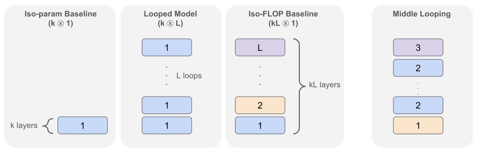
This is why a compact model can behave like a much deeper one while storing far fewer parameters. This structure is often written as \(k \otimes L\), meaning a \(k\)-layer block looped \(L\) times.
-
The following figure (source) shows the simple architecture-agnostic looping mechanism where a \(k\)-layer block looped \(L\) times, written as \(k \otimes L\), matches the effective depth of a \(kL\)-layer non-looped model while using far fewer distinct parameters.
Why It Matters
-
Looping separates two quantities that standard transformers usually conflate:
- Parameters: what the model can store.
- Computation: how much processing the model performs on a specific input.
-
FAIR’s Which one is more important: more parameters or more computation? frames this distinction directly, arguing that compute and parameter count should be treated as separate design axes. This is central to looped transformers: parameter count remains fixed, while FLOPs grow with the number of loops.
-
As a result:
- Parameter efficiency comes from reusing the same block instead of storing many unique layers.
- Runtime depth control allows more loops to be run for harder inputs.
- Latent reasoning refines hidden states internally without emitting intermediate tokens.
- Algorithmic structure lets the model resemble iterative procedures such as search, optimization, and multi-hop composition.
- Deployment efficiency improves because memory footprint remains much smaller than an equally deep non-looped model.
-
This is especially attractive for inference, where parameter storage, memory bandwidth, and activation movement often dominate deployment cost.
Latent Reasoning
-
Recent reasoning systems often improve performance by generating longer chain-of-thought outputs. That approach externalizes reasoning into text, which increases sequence length, latency, and context usage.
-
Looped transformers provide a different route: they reason internally in continuous latent space. Instead of producing intermediate tokens, the model repeatedly refines its hidden state:
-
Each loop acts like another internal computation step before the model emits the next token. Scaling up Test-Time Compute with Latent Reasoning by Geiping et al. (2025) demonstrates that recurrent-depth language models can improve at inference time by running additional loops, effectively increasing reasoning compute without generating longer chain-of-thought text.
-
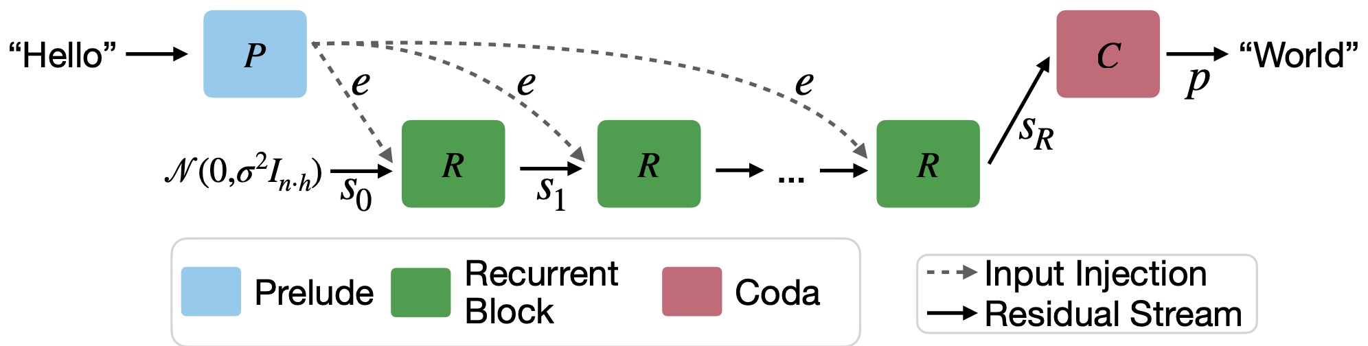
The following figure (source) shows a visualization of the architecture. Each block consists of a number of sub-layers. The blue prelude block embeds the inputs into latent space, where the green shared recurrent block is a block of layers that is repeated to compute the final latent state, which is decoded by the layers of the red coda block.
-
Unlike chain-of-thought, these intermediate states are never decoded into text. This enables more compact reasoning, non-linguistic internal search, better compute efficiency, and reasoning trajectories that do not need to be human-readable. Training Large Language Models to Reason in a Continuous Latent Space by Hao et al. (2025) introduces Coconut, showing that continuous latent states can encode multiple possible reasoning branches rather than committing immediately to a single text-token path.
-
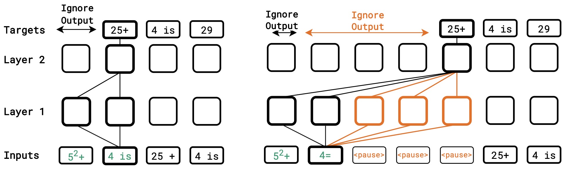
The following figure (source) shows (left) standard inference and finetuning and (right) pause-inference and pause-finetuning for a decoder-only model on a downstream task, where the model attends to the full prefix before generating the target answer. Rounded squares denote Transformer operations consisting of self-attention and MLP layers in a 2-layer Transformer. “Ignore Output” means that the corresponding output token is not extracted during inference, is not fed back autoregressively, and is not backpropagated through during finetuning. The connecting lines show selected computational pathways from the prefix token “4 is” to the output token “25+”. In the standard setting, output extraction begins immediately after the final prefix token; in the pause setting, manually inserted
<pause>tokens delay output extraction and create additional colored computational pathways between the prefix and the target answer.
Iterative Computation
-
Many hard tasks are naturally iterative: multi-hop retrieval, graph search, gradient descent, constraint propagation, planning, and dynamic programming all involve repeated updates to an internal state.
-
Looped transformers match this structure directly:
\[h_{t+1}=\mathcal{A}_{\theta}(h_t)\]- where \(\mathcal{A}_{\theta}\) is a learned update rule. The recurrent block becomes one computational step, and looping becomes the control mechanism that repeatedly executes that step.
-
Looped Transformers Are Better at Learning Learning Algorithms by Yang et al. (2024) shows that looped models learn iterative solvers for regression and optimization tasks with less than 10% of the parameters required by comparable standard transformers. Looped Transformers as Programmable Computers by Giannou et al. (2023) extends this view by showing that a shallow transformer in a loop can simulate a small instruction-set computer.
-
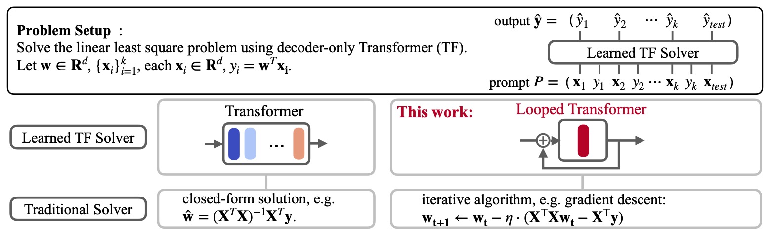
The following figure (source) shows how a transformer can be trained to learn an iterative learning algorithm for in-context linear regression, contrasting a learned transformer solver with an iterative gradient-descent-style solver. They consider the task of training a transformer to solve linear regression in context. The provided prompt \(\left(\boldsymbol{x}_1, y_1, \boldsymbol{x}_2, y_2, \cdots, \boldsymbol{x}_k, y_k, \boldsymbol{x}_{\text {test }}\right)\) is fed into a decoder transformer. The objective is to reduce the squared loss between the predicted \(\hat{y}_{\text {test }}\) based on this prompt, and the target value \(f\left(\boldsymbol{x}_{\text {test }}\right)\). What Can Transformers Learn In-Context? A Case Study of Simple Function Classes by Garg et al. (2022) demonstrated that a decoder transformer can learn to solve linear regression, which potentially involves learning the approximation of the least squares solution. In this study, we aim to train a transformer to learn iterative learning algorithms. Their goal is to achieve performance on par with standard transformers but with fewer paramtters. To this end, we introduce the looped transformer architecture and its accompanying training methodology.
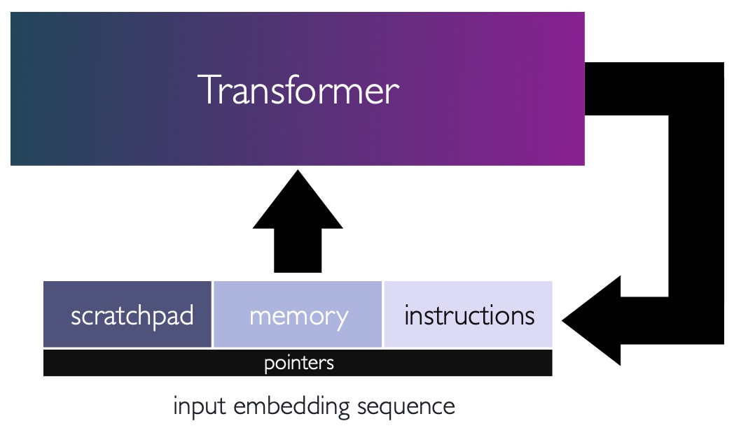
- The following figure (source) shows a looped transformer architecture, where the input sequence stores the commands, memory where the data is read/written from, and a scratchpad where intermediate results are stored. The input is processed by the network and the output is used as the new input, allowing the network to iteratively update an implicit state and perform complex computations.
Knowledge Use
-
A recurring lesson is that looped transformers often improve knowledge manipulation more than knowledge storage. Modern language models already store large amounts of information; the harder problem is combining facts, rules, and latent features in unfamiliar ways.
-
Scaling Latent Reasoning via Looped Language Models by Zhu et al. (2025) reports that Ouro models trained on up to 7.7 trillion tokens achieve performance competitive with larger non-looped models, with evidence that the advantage comes from stronger knowledge composition rather than simply greater memorization.
-
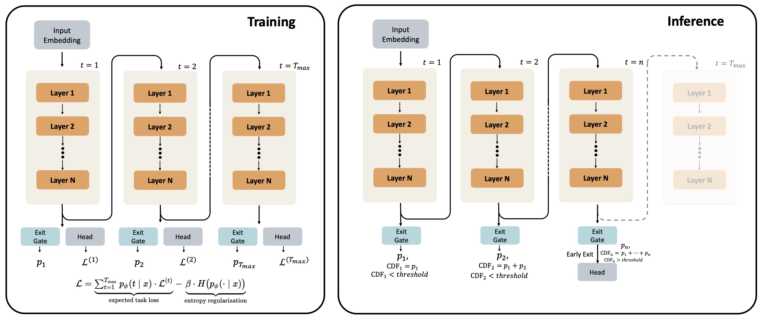
The following figure (source) shows an overview of the parameter-shared Looped Language Model (LoopLM) architecture. Left (Training): During training, the model applies a stack of \(N\) layers repeatedly for \(T_{max}\) recurrent steps. At each recurrent step \(l\), an exit gate predicts the probability \(p_l\) of exiting, and a language modeling head \(L_l\) computes the lanugage modeling loss. Right (Inference): At inference time, the model can exit early based on the accumulated exit probability.
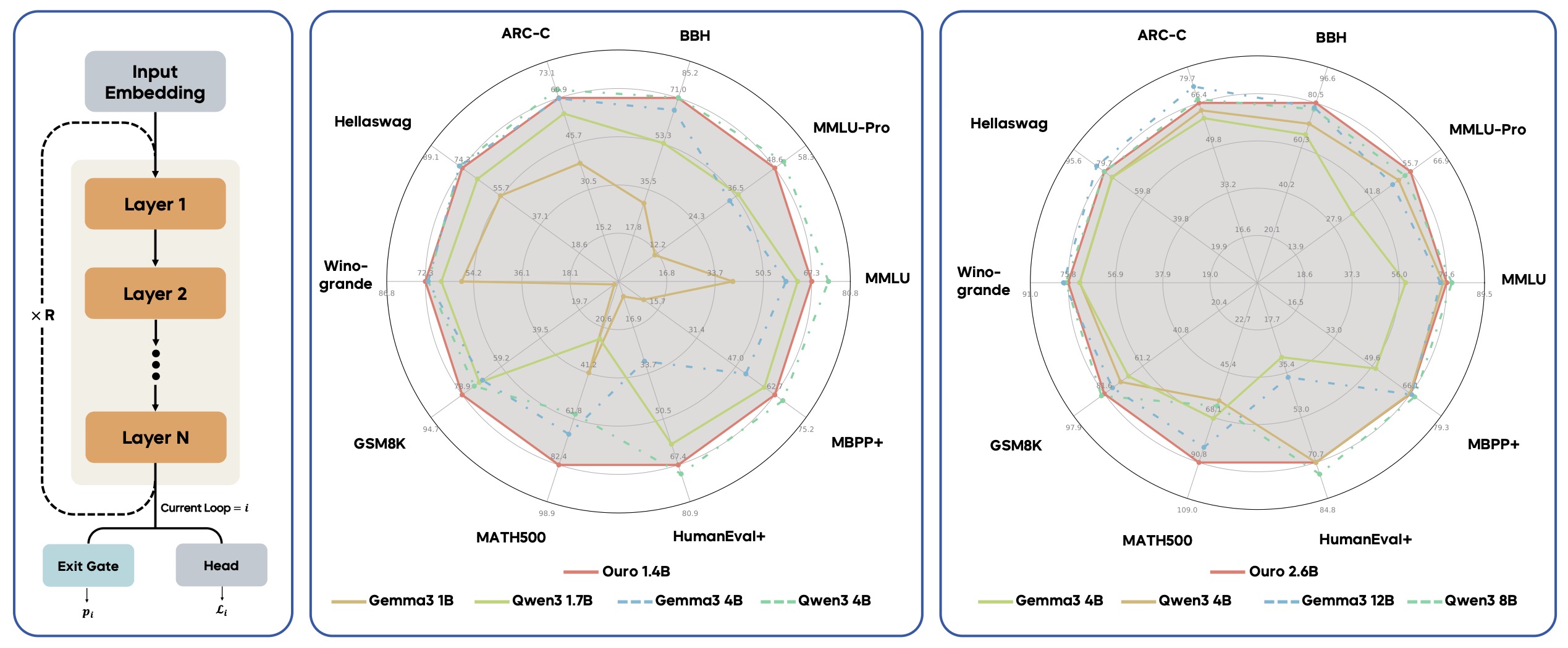
- The following figure (source) summarizes Ouro’s looped language model design and benchmark behavior. Left: the parameter-shared LoopLM architecture, where a stack of \(N\) layers is repeatedly applied for up to \(T_{\max}\) recurrent steps. During training, each recurrent step \(l\) has an exit gate that predicts the exit probability \(p_l\) and a language modeling head \(\mathcal{L}_l\) that contributes to the training loss; at inference time, the model can exit early based on the accumulated exit probability. Middle and right: radar plots comparing Ouro 1.4B and Ouro 2.6B, both using 4 recurrent steps, against individual transformer baselines. The results show that Ouro can reach performance comparable to, or better than, much larger baselines while using parameter sharing and recurrent latent computation.
- This makes looped transformers especially relevant for compositional reasoning: the model can repeatedly retrieve, transform, and combine internal information before committing to an output token.
Architecture
-
Looped transformers usually preserve the outer shape of a decoder-only language model while changing the depth structure. Instead of a long stack of unique layers, the model is commonly divided into three regions:
- Prelude: non-looped layers that prepare token representations.
- Recurrent core: one or more shared transformer blocks applied repeatedly.
- Coda: non-looped layers that convert the final recurrent state into logits.
-
A typical computation is:
-
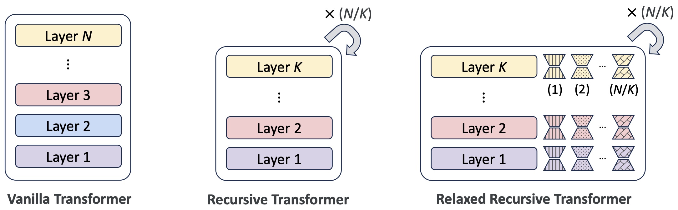
Relaxed Recursive Transformers: Effective Parameter Sharing with Layer-wise LoRA by Bae et al. (2025) uses this recursive-block view to convert pretrained transformers into smaller recursive models, then relaxes strict weight tying with layer-wise LoRA adapters.
-
The following figure (source) shows the conversion from a vanilla \(N\)-layer Transformer to a Recursive Transformer with \(\frac{N}{K}\) blocks of \(K\) shared layers, and then to a Relaxed Recursive Transformer with layer-specific LoRA modules.
Shared Core
- The recurrent core is typically a standard transformer block or stack. In a residual formulation, one loop step can be written as:
- In implementation, this means the same module object is called repeatedly inside a loop:
for step in range(num_loops):
    hidden_states = recurrent_block(
        hidden_states,
        attention_mask=attention_mask
    )
- The key detail is that
recurrent_blockhas one shared set of weights. Gradients from all loop steps accumulate into the same parameters during backpropagation.
Modern Looping Topologies
Full-stack looping
- The simplest modern realization of recurrent depth is full-stack looping: after a hidden state traverses the Transformer stack once, the resulting state is sent through the same stack again. If the shared stack is represented by \(F_{\theta}\), a two-pass model computes:
-
The effective computation resembles a Transformer with twice the depth, but both passes use the same parameters \(\theta\).
-
Nanbeige4.2-3B: Unlocking Agentic Capabilities in a Compact Model by Yang et al. (2026) is a large-scale example of this design: the model is pretrained from scratch on \(28\) trillion tokens and sends hidden states through the same Transformer stack for an additional pass, increasing effective computational depth without introducing another copy of the layer parameters.
-
This design can be interpreted as converting a stack of \(k\) unique layers into an effective depth of:
\[D_{\mathrm{eff}} = kR\]- where \(R\) is the number of full-stack passes. Nanbeige4.2 uses the especially simple case in which the shared stack is traversed twice. The architecture therefore separates stored depth from executed depth: stored parameters correspond to one stack, whereas the forward pass executes the stack repeatedly.
-
Training the recurrence from the beginning appears important in this setting. Nanbeige4.2-3B: Unlocking Agentic Capabilities in a Compact Model by Yang et al. (2026) reports that pretraining the looped architecture from scratch performs substantially better than first training a conventional Transformer and then introducing the additional pass. This suggests that the representations themselves adapt to being repeatedly processed by the same transformation.
-
The same experiments also illustrate why loop count is an architectural hyperparameter rather than a monotonically beneficial scaling knob. A two-pass configuration provided the best reported trade-off, retaining approximately 75% of the token efficiency of the corresponding standard Transformer while adding substantial effective capacity; additional passes produced only marginal gains while making optimization slower and less stable.
Recurrent-core looping
-
Full-stack recurrence is not required. A model can instead retain unique layers around a smaller recurrent middle section:
\[h_0 = P_{\theta_P}(x)\] \[h_{r+1} = F_{\theta_R}(h_r), \qquad r=0,\ldots,R-1\] \[y = C_{\theta_C}(h_R)\]- where \(P_{\theta_P}\) is a non-recurrent prelude, \(F_{\theta_R}\) is the shared recurrent core, and \(C_{\theta_C}\) is a non-recurrent coda.
-
Scaling up Test-Time Compute with Latent Reasoning: A Recurrent Depth Approach by Geiping et al. (2025) uses this decomposition to place a repeatedly executed block between non-recurrent input and output processing. The recurrent state remains in latent space, allowing inference compute to increase by unrolling the shared core for additional iterations without requiring additional reasoning tokens.
-
A recurrent middle block can be preferable to looping the complete model because the surrounding layers can specialize. The prelude can map token embeddings into a representation suited to repeated refinement, the recurrent core can learn an iterative update rule, and the coda can translate the final recurrent representation into the distribution required by the language-modeling head.
-
This architecture also makes inference-time depth especially natural:
\[h_R = F_{\theta_R}^{\,R}(h_0)\]- where the exponent denotes repeated function composition rather than exponentiation. The same checkpoint can therefore expose different compute budgets by changing \(R\), provided that training has produced recurrent dynamics that remain useful beyond the nominal training depth. [Scaling up Test-Time Compute with Latent Reasoning: A Recurrent Depth Approach] by Geiping et al. (2025) demonstrates continued reasoning improvements under increased recurrent computation, including at compute loads substantially above the model’s stored parameter scale.
Block looping vs. layer looping
-
Recurrence can be applied at an even finer granularity. Suppose a recurrent window contains layers \(L_a,L_{a+1},\ldots,L_b\). There are at least two structurally different ways to repeat it.
-
Block-mode recurrence repeats the entire sequence of layers:
- Layer-mode recurrence repeats each individual layer before progressing to the next:
-
These computations have similar nominal effective depth but are not functionally equivalent because the order of repeated transformations changes. Training-Free Looped Transformers by Chen et al. (2026) explicitly studies both arrangements while adding recurrence to frozen pretrained checkpoints without updating their parameters.
-
The distinction becomes particularly important for Mixture-of-Experts models. In block mode, repeatedly traversing an entire multi-layer region allows representations to reach the same MoE layer in substantially changed states on every pass, which can cause expert assignments to change repeatedly. [Training-Free Looped Transformers] by Chen et al. (2026) reports that layer-mode iteration is the safer default for MoE backbones because repeated applications remain localized within a particular layer, reducing cross-iteration expert-routing instability.
-
More broadly, this shows that “number of loops” does not fully specify a recursive architecture. Two models with the same parameter count and nominal effective depth can implement very different computations depending on whether recurrence is applied to a single layer, a contiguous group of layers, a complete stack, or an independently designed recurrent core.
Training-free recurrence
-
Most recurrent-depth models are trained with parameter sharing present throughout pretraining. Training-Free Looped Transformers by Chen et al. (2026) explores the complementary question: whether useful recurrence can be introduced only at inference time into an ordinary frozen Transformer.
-
Naively repeating a pretrained block generally degrades performance because the block was optimized to make one residual update, not to consume its own output repeatedly. Chen et al. reinterpret a pre-norm Transformer residual block as a numerical integration step:
\[h_{t+1} = h_t + F_{\theta}(h_t)\]- which resembles a forward-Euler step for an underlying dynamical system.
-
Instead of applying that full update \(K\) times, the recurrence can be interpreted as subdividing one update into smaller steps:
-
This perspective attempts to keep the recurrent trajectory near the transformation that the pretrained model already learned, rather than allowing repeated full residual updates to move the representation arbitrarily far away. The reported method loops a contiguous middle region of a frozen model using numerical-integration-inspired update strategies and obtains improvements across multiple dense and MoE checkpoints without additional parameter training.
-
Training-free looping therefore occupies a different point in the design space. Native looped models learn the recurrent dynamics during pretraining, whereas training-free methods attempt to construct stable recurrence from the dynamics already present in an ordinary checkpoint.
Token-adaptive recurrence
-
Fixed-loop architectures assign the same depth to every token \(R_i=R \forall i\), but this can waste computation because different positions may require different amounts of refinement.
-
Mixture-of-Recursions: Learning Dynamic Recursive Depths for Adaptive Token-Level Computation by Bae et al. (2025) combines shared recurrent parameters with lightweight routing so each token can receive its own recursion depth.
-
A simplified formulation assigns token \(i\) a recursion budget:
\[R_i = g_{\phi}(h_i)\]- and defines whether the token remains active at recurrent step \(r\) as:
-
If \(n_r\) tokens remain active at recurrence \(r\), full fixed-depth recurrence pays attention cost on all \(n\) tokens at every step \(C_{\mathrm{fixed}} \propto R n^2\), whereas an idealized adaptive implementation pays approximately \(C_{\mathrm{adaptive}} \propto \sum_{r=1}^{R} n_r^2\) with \(n_{r+1}\leq n_r\) as progressively more tokens exit.
-
[Mixture-of-Recursions: Learning Dynamic Recursive Depths for Adaptive Token-Level Computation] by Bae et al. (2025) explicitly restricts quadratic attention computation to tokens that remain active at a given recursive depth and selectively caches the corresponding key-value pairs. Across models ranging from \(135\)M to \(1.7\)B parameters, the paper reports a Pareto improvement over vanilla and prior recursive baselines in validation perplexity, few-shot accuracy, model size, and throughput at comparable training-compute budgets.
-
This architecture can be understood as a depth analogue of sparse expert routing. Mixture-of-Experts chooses which parameterized expert processes a token, whereas Mixture-of-Recursions chooses how long the token continues to be processed by a shared recurrent computation.
Mixture-of-Experts with recurrence
-
Recurrence and expert sparsity are complementary. In an MoE recurrent layer, the shared transformation can be written schematically as:
\[h_i^{(r+1)} = \sum_{e\in\mathcal{E}} \pi_e \left( h_i^{(r)} \right) F_{\theta_e} \left( h_i^{(r)} \right)\]- where \(\pi_e\) represents the router and only a sparse subset of experts is typically activated.
-
Although the expert parameters are reused across recurrent depth, expert selection can vary because the representation \(h_i^{(r)}\) changes from one recurrence to the next. Recurrence therefore does not necessarily mean performing the identical computation repeatedly: the shared routing function may send the evolving hidden state through different expert pathways.
-
Loop the Loopies! by Gao et al. (2026) develops this direction with the Loopie family of MoE models, including a \(20\)B-parameter model with \(2\)B active parameters and a \(6\)B model with \(0.6\)B active parameters. The work is motivated by the observation that simply spending an \(N\)-fold larger pretraining budget by looping a model \(N\) times has historically been weaker than using that budget to increase unique parameter count, and reports looped MoE designs that outperform compute-matched vanilla Transformer baselines.
-
This introduces two independent forms of conditionality:
\[\text{depth routing} \quad+\quad \text{expert routing}\]- where depth routing determines how many transformations a token receives and expert routing determines which sparse parameters implement those transformations.
Parallel loop transformers
-
Ordinary recurrence is sequential along the loop dimension \(h_i^{(1)} \rightarrow h_i^{(2)} \rightarrow \cdots \rightarrow h_i^{(R)}\) so \(R\) recurrent passes ordinarily create approximately \(R\) serial executions for each generated token. Weight sharing saves parameter memory but does not by itself eliminate this latency.
-
Parallel Loop Transformer for Efficient Test-Time Computation Scaling by Wu et al. (2025) introduces Cross-Loop Parallelism, which pipelines recurrence across neighboring autoregressive tokens. Instead of computing every recurrence for one token before beginning the next, the system concurrently computes an early recurrence for a newer token and later recurrences for older tokens.
-
With three loops, a decoding micro-batch can conceptually contain \(\left\{h_i^{(1)},h_{i-1}^{(2)},h_{i-2}^{(3)}\right\}\) so three different recurrent stages are executed together. The architecture breaks the same-token cross-loop dependency by shifting the preceding loop’s states by one sequence position before adding the original token embeddings.
-
The resulting trade-off is unusual. The amount of arithmetic remains approximately \(C_{\mathrm{PLT}} \approx R C_{\mathrm{base}}\) because all recurrent computations still occur, but under the memory-bound decoding assumptions studied in the paper, their execution is overlapped so the reported critical decoding latency remains close to that of a single loop rather than increasing proportionally with \(R\).
KV sharing in parallel recurrence
-
Parallelizing the recurrent passes solves only one systems bottleneck. If every recurrence stores independent key-value states, the vanilla cache cost remains approximately \(M_{\mathrm{KV}}=\mathcal{O} \left(Rnd \right)\) for sequence length \(n\), hidden dimension proportional to \(d\), and \(R\) recurrent passes.
-
[Parallel Loop Transformer for Efficient Test-Time Computation Scaling] by Wu et al. (2025) therefore shares the first loop’s global KV cache across later loops. Later recurrences retain their own queries but attend globally to \(K_{\mathrm{share}}, V_{\mathrm{share}}\) instead of storing a full independent global cache at every recurrent depth.
-
Because complete KV sharing loses recurrence-specific local information, non-first loops additionally perform sliding-window attention using their private keys and values:
- A learned sigmoid gate combines the two:
- This changes the cache complexity from the vanilla recurrent form \(\mathcal{O}(Rnd)\) to \(\mathcal{O}\left(nd+(R-1)wd\right)\), where \(w\) is the sliding-window length and is much smaller than the total sequence length in the intended regime.
Loop count in parallel architectures
-
Parallel recurrence removes much of the wall-clock penalty of adding loops, but it does not imply that arbitrarily many loops improve quality. LoopCoder-v2: Only Loop Once for Efficient Test-Time Computation Scaling by Yang et al. (2026) trains matched \(7\)B Parallel Loop Transformer coding models from scratch on \(18\) trillion tokens specifically to study loop-count selection.
-
The two-loop variant produced large improvements over the non-looped baseline, including SWE-bench Verified increasing from \(43.0\) to \(64.4\) and Multi-SWE from \(14.0\) to \(31.0\). Models using three or more loops instead regressed. The paper’s diagnostics indicate that the second pass supplies the dominant useful refinement, while subsequent loops produce progressively smaller and more oscillatory state changes with reduced representational diversity.
-
This suggests a useful gain-cost view of recursive depth:
\[\Delta Q_r = G_r-C_r\]- where \(G_r\) denotes the useful representational refinement contributed by recurrence \(r\) and \(C_r\) denotes architectural costs such as positional mismatch, optimization instability, or loss of representation diversity.
-
Additional recurrence is beneficial only while \(G_r>C_r\) and optimal depth can therefore occur at a surprisingly small recurrence count even when parallel hardware makes additional FLOPs inexpensive.
The design space
- These architectures show that “looped Transformer” describes a family rather than one fixed topology. The major design choices are orthogonal:
| Design axis | Representative choices |
|---|---|
| Recurrent scope | individual layer, layer window, recurrent core, entire stack |
| Application order | block-wise recurrence, layer-wise recurrence |
| Depth allocation | fixed globally, adaptive per sequence, adaptive per token |
| Parameterization | strictly shared, relaxed sharing, sparse MoE |
| Training | from scratch, uptrained, training-free |
| Scheduling | sequential loops, cross-token parallel loops |
| KV strategy | independent per loop, selectively cached, shared, shared plus local window |
| Output policy | final-loop prediction, intermediate heads, learned early exit |
- The architectural question is therefore not merely how many times a Transformer should loop. It is which computation should recur, which state should be propagated between recurrences, whether different tokens should receive different depths, whether parameter or expert routing should change between iterations, and how the resulting computation should be scheduled on inference hardware.
Effective Depth
- If the recurrent core contains \(k\) layers and is executed for \(L\) loops, the effective depth is:
- This allows a compact model to behave like a much deeper one while storing far fewer parameters. Looped Transformers Are Better at Learning Learning Algorithms by Yang et al. (2024) shows that repeated structure is especially useful for learning iterative algorithms such as regression solvers.
Weight Tying
-
The defining implementation choice is how aggressively weights are tied.
-
Strict tying uses the exact same attention, MLP, normalization, and projection weights at every loop step:
-
Relaxed tying adds small step-specific adapters:
\[\theta_t=\theta+\Delta\theta_t\]- where \(\Delta\theta_t\) is often low-rank. Relaxed Recursive Transformers: Effective Parameter Sharing with Layer-wise LoRA by Bae et al. (2025) uses LoRA modules to preserve most memory savings while recovering performance lost from strict parameter sharing.
Loop Count
-
Loop count can be fixed, sampled, or learned.
-
A fixed-depth setup uses the same loop count during training and inference:
- A test-time scaling setup trains on one depth or a range of depths, then increases recurrence during inference:
-
Loop, Think, & Generalize: Implicit Reasoning in Recurrent-Depth Transformers by Kohli et al. (2026) shows that increasing recurrence at inference time can unlock depth extrapolation on multi-hop reasoning tasks.
-
The following figure (source) shows the recurrent-depth model architecture where a shared transformer block is repeated \(R\) times before layer normalization and the language-model head. The embedding layer and language model head (LM Head) have tied weights. In their experiments, they use a simple looped transformer similar to Reasoning with Latent Thoughts: On the Power of Looped Transformers Saunshi et al. (2025), without design elements such as input injection, gated halting, and middle looping.

- A learned early-exit setup predicts whether each token or sequence needs more computation. Mixture-of-Recursions: Learning Dynamic Recursive Depths for Adaptive Token-Level Computation by Bae et al. (2025) introduces token-level routing so different tokens can receive different recursion depths.
Output Heads
- Most looped language models apply the language modeling head only after the final loop:
- Adaptive-depth models may attach auxiliary heads at intermediate loops:
- These intermediate predictions can support early exit, depth supervision, confidence-based routing, or learned compute allocation. Scaling Latent Reasoning via Looped Language Models by Zhu et al. (2025) uses an exit mechanism so computation can be allocated dynamically rather than uniformly.
Training
-
Training looped transformers requires more than tying weights and repeatedly calling the same block. Because the same parameters are reused across many iterations, the model is optimized through a deeper computational graph than its parameter count suggests, and training must teach the recurrent block to refine representations progressively rather than solve the prediction problem in one static pass.
-
The training objective is usually the standard autoregressive language modeling loss:
\[\mathcal{L}_{\text{LM}} =-\sum_{t=1}^{T} \log p(x_t \mid x_{<t})\]- where the probability distribution is computed from the final recurrent state after \(L\) loop iterations. Even though the loss is familiar, recurrence changes the optimization dynamics because every loop contributes gradients to the same shared weights.
Depth Sampling
-
A central training decision is whether to use a fixed loop count or sample loop counts during training. If a model is always trained with the same recurrence depth, it may become brittle when evaluated with fewer or more loops. A more flexible approach samples the number of iterations:
\[L \sim p(L)\]- where \(p(L)\) may be uniform over a bounded range, biased toward shorter depths early in training, or gradually expanded as the model stabilizes.
-
This teaches the model to produce useful representations after a small number of iterations while still benefiting from additional computation when more loops are available. Scaling up Test-Time Compute with Latent Reasoning by Geiping et al. (2025) uses recurrent-depth training so the model can exploit increased inference-time recurrence for latent reasoning. Parcae: Scaling Laws for Stable Looped Language Models by Prairie et al. (2026) studies this compute axis systematically and shows that loop count can follow predictable scaling behavior when training is stable.
Progressive Refinement
- The recurrent block is best understood as a learned refinement operator. Rather than treating each layer as a different stage of processing, the same function is applied repeatedly so that the hidden state becomes progressively more useful:
-
Ideally, each iteration reduces prediction error or improves the internal representation:
\[\mathcal{E}(h_{t+1}) \leq \mathcal{E}(h_t)\]- where \(\mathcal{E}\) denotes an implicit task error. This is why looped transformers naturally resemble iterative procedures such as gradient descent, graph search, message passing, and constraint propagation. Looped Transformers Are Better at Learning Learning Algorithms by Yang et al. (2024) shows that looped architectures are particularly effective at learning iterative optimization behavior with far fewer parameters than standard transformers.
Multi-Step Supervision
- Some looped models apply loss only after the final iteration:
-
This keeps the training objective simple and encourages the final state to be maximally predictive. Other recipes attach auxiliary prediction heads to intermediate loop states and train with a weighted sum:
\[\mathcal{L} =\sum_{t=1}^{L} w_t \mathcal{L}_t\]- where \(\mathcal{L}_t\) is the language modeling loss after loop \(t\). Intermediate supervision can improve gradient flow, make early exits more reliable, and encourage every recurrence step to produce a meaningful refinement rather than relying only on the final iteration.
-
Scaling Latent Reasoning via Looped Language Models by Zhu et al. (2025) combines recurrent pretraining with learned depth allocation, so the model is trained not only to predict tokens but also to decide how much latent computation is useful.
Exit and Routing Losses
-
When a looped model supports early exit or token-level adaptive depth, training usually adds objectives that make computation allocation learnable. A simple form penalizes excessive recurrence:
\[\mathcal{L} =\mathcal{L}_{\text{LM}} + \lambda \mathbb{E}[L]\]-
where \(\mathbb{E}[L]\) is the expected number of recurrent steps. Entropy regularization may also be used so the routing mechanism does not collapse into always exiting early or always using maximum depth:
\[\mathcal{L} =\mathcal{L}_{\text{LM}} - \beta H(p)\]
-
-
Mixture-of-Recursions: Learning Dynamic Recursive Depths for Adaptive Token-Level Computation by Bae et al. (2025) extends adaptive computation to the token level, allowing different tokens in the same sequence to receive different recursion depths.
Uptraining from Existing Models
- A practical way to build looped transformers is to convert an existing pretrained transformer into a recursive model. Suppose the original model contains layers \(\theta_1,\dots,\theta_N\). A shared recurrent block can be initialized by selecting representative layers, averaging compatible layers, or compressing several layers into a smaller repeated block:
- After tying the layers, the model is uptrained so it can adapt to repeated use of the same block. This avoids training from scratch and makes looped architectures more practical for modern language models. Relaxed Recursive Transformers: Effective Parameter Sharing with Layer-wise LoRA by Bae et al. (2025) shows that pretrained transformers can be converted into recursive models and then improved with layer-wise LoRA adapters that partially relax strict weight tying.
Depth Curriculum
-
Training often benefits from gradually increasing recurrence depth. Early in training, short loops reduce instability and help the block learn basic transformations; later, longer loops teach the model to sustain useful computation across many applications of the same weights.
-
A simple schedule is:
\[L_{\max}(s) =\min(L_{\text{target}}, L_0 + ks)\]- where \(s\) is the training step, \(L_0\) is the initial loop budget, and \(k\) controls how quickly the maximum depth grows. Loop, Think, & Generalize: Implicit Reasoning in Recurrent-Depth Transformers by Kohli et al. (2026) shows that training strategy strongly affects whether recurrent-depth transformers can extrapolate to deeper multi-hop reasoning than they saw during training.
Inference Scaling
- A defining advantage of looped transformers is that inference-time compute can be increased after training by running more loop iterations:
-
Performance often improves with additional loops before saturating. A useful empirical shape is:
\(\epsilon\)L\(\approx \epsilon_\infty + A e^{-kL}\)
- where \(\epsilon(L)\) is error after \(L\) loops, \(\epsilon_\infty\) is the asymptotic error, and \(A e^{-kL}\) captures diminishing returns. Parcae: Scaling Laws for Stable Looped Language Models by Prairie et al. (2026) characterizes this behavior and treats looping as a predictable compute-scaling axis.
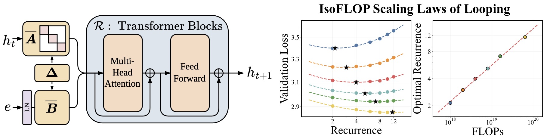
-
The following figure shows Parcae stabilizing recurrent dynamics and establishing looping as a scaling axis for increased computation. (Left) Parcae constrains the spectral norm of \(A\) and normalizes the input injection, stabilizing the residual stream \(h_t\) across loops. (Right) We observe looping to be an orthogonal axis of scaling compute which follows a power law.
Training Setup
-
In implementation, looped models usually require careful choices around recurrence depth, normalization, optimization, and memory management. Loop counts during training commonly span a modest range and may be increased at inference; the shared recurrent core is often a small stack of transformer layers rather than a single layer; normalization is usually placed before attention and feed-forward sublayers to stabilize repeated application; gradient clipping is commonly needed because the unrolled graph can amplify updates; the learning rate is often set more conservatively than for a comparable non-looped model; mixed precision is typically used as in standard LLM training; and activation checkpointing becomes important because activation memory grows with the number of unrolled iterations unless recomputation is used.
-
The broader training philosophy is that a looped transformer learns a reusable computational step. Instead of learning a fixed sequence of specialized layers, it learns a transformation that can be applied repeatedly to move an internal state closer to a useful answer.
Stability
- Stability is one of the hardest practical problems in looped transformers. Reusing the same block many times can amplify small errors, cause residual states to grow uncontrollably, or produce loss spikes during training. A looped transformer is therefore not just a transformer with shared weights; it is a dynamical system whose behavior depends on what repeated application of the same transformation does to the residual stream.
Dynamics
-
A useful abstraction writes the recurrent update as:
\[h_{t+1} =A h_t + B e + R(h_t,e)\]- where \(h_t\) is the residual state at loop step \(t\), \(e\) is the input embedding or conditioning signal, \(A\) controls how much of the previous residual state is retained, \(B\) controls how strongly the input is injected at each step, and \(R(h_t,e)\) represents nonlinear transformer operations such as attention and the MLP.
-
Parcae: Scaling Laws for Stable Looped Language Models by Prairie et al. (2026) uses this dynamical-systems view to explain why looped models can become unstable, identifying large spectral norms in injection parameters as a major source of residual explosion.
Residual Growth
-
If the recurrent transformation expands hidden states, then repeated looping magnifies the expansion. In a simplified linear system \(h_{t+1}=Ah_t\), the state after \(L\) loops is \(h_L=A^L h_0\).
-
If the spectral radius of \(A\) exceeds 1, then the norm of \(h_L\) can grow exponentially with \(L\). This is the core mathematical reason looped architectures are more fragile than ordinary feed-forward transformer stacks: the same unstable transformation is applied repeatedly rather than only once.
-
A stable looped model should keep the recurrent update contractive or at least norm-controlled:
\[\rho(A) \leq 1\]- where \(\rho(A)\) is the spectral radius. In practice, exact spectral control over the full nonlinear transformer is difficult, so implementations use normalization, residual scaling, careful initialization, and constrained parameterizations.
Normalization
-
Normalization is central because the same block sees its own outputs repeatedly. Pre-norm transformers are usually preferred because they normalize the input to each attention and MLP operation before the update is applied. A simplified pre-norm recurrent block can be written as:
\[h_{t+1} =h_t +\alpha F_\theta(\text{Norm}(h_t))\]- where \(\alpha\) is a residual scale. Smaller \(\alpha\) can prevent each loop from making overly large updates, while normalization keeps the input distribution to the shared block more consistent across loop iterations.
-
Post-norm can sometimes damp the final output of a block, but repeated post-norm architectures may still suffer from unstable intermediate dynamics. Parcae: Scaling Laws for Stable Looped Language Models by Prairie et al. (2026) specifically motivates stabilizing the residual stream rather than relying only on ordinary transformer normalization.
Injection
-
A subtle issue in looped models is whether the original input is injected once or repeatedly. If the input is only used to initialize (h_0), then later loops may drift away from the original prompt. If the input is injected at every step, the model receives persistent conditioning, but the repeated injection can destabilize the residual stream if its magnitude is uncontrolled.
-
The recurrent update with input injection is:
- Stable architectures therefore need to control both the memory term \(A h_t\) and the injection term \(B e\). Parcae: Scaling Laws for Stable Looped Language Models by Prairie et al. (2026) proposes constraining injection parameters through a negative diagonal parameterization and discretization, which is designed to prevent repeated input injection from causing residual explosion.
Loss Spikes
-
Loss spikes can arise when stochastic depth training exposes the model to loop counts it is not yet stable under. A model may perform well at \(L=4\) but become unstable at \(L=16\), and if training randomly samples \(L=16\), the resulting gradient can be large enough to destabilize the shared weights for all depths.
-
This is why depth curricula, gradient clipping, conservative learning rates, and activation norm monitoring are more important in looped transformers than in ordinary transformers. The repeated block must remain useful not only for the depths used in the current batch, but also for the range of depths expected at inference.
Overthinking
-
More recurrence is not always better. A looped model may improve for several iterations and then degrade if additional loops push the representation away from the correct answer. This failure mode is often called overthinking.
-
In qualitative terms, the model first refines its answer, then begins to overwrite or distort useful information. Formally, accuracy as a function of loop count may rise and then fall rather than monotonically saturate:
\(\text{Acc}(L+1) < \text{Acc}\)L\(\)
- for sufficiently large \(L\). Loop, Think, & Generalize: Implicit Reasoning in Recurrent-Depth Transformers by Kohli et al. (2026) identifies overthinking as a limitation of recurrent-depth transformers, especially when recurrence is pushed far beyond the training regime.
Stabilization
-
A stable implementation typically treats recurrence as a controlled iterative process. The residual update should be small enough to avoid explosion, normalization should keep hidden-state statistics consistent across loops, input injection should be bounded, and the training distribution over loop counts should expose the model gradually to deeper computation.
-
A practical recurrent block often resembles:
\[h_{t+1} =h_t +\alpha_t F_\theta(\text{RMSNorm}(h_t))\]- where \(\alpha_t\) may be fixed, learned, or scheduled. The purpose of \(\alpha_t\) is to make each loop behave like a refinement step rather than a full independent layer. This design aligns looped transformers more closely with stable iterative algorithms, where each update is controlled to avoid divergence.
Scaling Laws
-
One of the most important developments in looped transformers is the discovery that recurrence follows predictable scaling laws. Just as conventional language models obey power laws relating loss to parameters, data, and training FLOPs, looped transformers reveal that increasing recurrence depth forms an additional and largely orthogonal axis of scaling. This means that model quality can be improved by allocating more computation to repeated applications of a fixed parameter set, without increasing the number of stored weights.
-
Parcae: Scaling Laws for Stable Looped Language Models by Prairie et al. (2026) provides the most systematic treatment of this phenomenon, deriving empirical laws for both training-time and inference-time scaling in stable looped language models.
Compute Axis
-
Traditional scaling laws treat model performance as a function of parameter count \(N\), dataset size \(D\), and total training compute \(C\). In standard transformers, increasing compute usually implies increasing parameters or training on more data. Looped transformers introduce a new factor, recurrence depth \(L\), which increases FLOPs while keeping parameter count fixed:
\[C \propto N D L\]- where \(N\) is the number of unique parameters, \(D\) is the amount of training data, and \(L\) is the average number of recurrent steps.
-
This decoupling makes it possible to ask a new question: given a fixed parameter budget, how should compute be divided between additional data and additional looping? Parcae: Scaling Laws for Stable Looped Language Models by Prairie et al. (2026) shows that optimal performance is achieved by increasing both data and recurrence together rather than relying exclusively on one or the other.
Effective Depth
- A looped model with \(k\) shared layers executed \(L\) times has effective depth:
-
Empirically, many reasoning and language modeling tasks depend more strongly on effective depth than on the number of distinct parameter sets. Reasoning with Latent Thoughts: On the Power of Looped Transformers by Saunshi et al. (2025) shows that looped and non-looped models often align when compared at equal effective depth, suggesting that recurrent computation can substitute for explicit stacking.
-
This observation is especially significant for reasoning tasks, where multi-step compositional computation appears to be the limiting factor rather than raw memorization capacity.
Training Scaling
-
When recurrence is treated as a variable rather than a fixed architectural choice, training loss follows predictable power-law behavior analogous to standard scaling laws:
\[\mathcal{L}(C) \approx a C^{-b} + c\]- where \(C\) includes FLOPs contributed by recurrent iterations.
-
The implication is that looping behaves as a first-class scaling mechanism rather than an architectural curiosity. Additional recurrence can be traded against increased model size or additional data while preserving predictable improvements. Parcae: Scaling Laws for Stable Looped Language Models by Prairie et al. (2026) demonstrates that stable looped models obey smooth and predictable loss curves as recurrence and data are scaled jointly.
Inference Scaling
- Looped transformers are especially notable because recurrence can be increased after training. If a model was trained on a range of loop counts, inference can use larger values:
-
Performance typically improves with diminishing returns, following a saturating exponential:
\[\epsilon(L) \approx \epsilon_\infty +A e^{-kL}\]- where \(\epsilon(L)\) is the task error after \(L\) loops.
-
This behavior closely parallels the scaling of chain-of-thought reasoning, except that the additional computation occurs entirely in latent space rather than through token generation. Scaling up Test-Time Compute with Latent Reasoning by Geiping et al. (2025) shows dramatic benchmark improvements when inference-time recurrence is increased, particularly on tasks such as GSM8K and ARC Challenge.
Compute Allocation
-
An important consequence of recurrence-based scaling is that computation can be allocated dynamically rather than uniformly. Some inputs may converge after only a few iterations, while others benefit from substantially more depth. Learned exit mechanisms and routing modules therefore turn recurrence into a per-input or per-token compute budget.
-
Scaling Latent Reasoning via Looped Language Models by Zhu et al. (2025) uses entropy-regularized exit probabilities to allocate computation adaptively across examples. Mixture-of-Recursions: Learning Dynamic Recursive Depths for Adaptive Token-Level Computation by Bae et al. (2025) generalizes this idea by allowing individual tokens to stop recurring at different depths.
-
This adaptive strategy effectively replaces the fixed-depth assumption of standard transformers with a learned, input-dependent computational schedule.
Parameter Efficiency
-
Because recurrence increases FLOPs without increasing stored weights, looped transformers occupy a favorable point on the trade-off between memory footprint and computational power. A smaller model with additional recurrence can often match a much larger standard transformer.
-
Scaling Latent Reasoning via Looped Language Models by Zhu et al. (2025) reports that Ouro models with 1.4B and 2.6B parameters perform competitively with models several times larger, while Parcae: Scaling Laws for Stable Looped Language Models by Prairie et al. (2026) shows that a 1.3B looped model achieves up to 87.5% of the quality of a transformer twice its size.
Scaling Interpretation
- The broader interpretation is that model quality depends on three largely independent resources:
-
Looped transformers expose computation as a directly controllable variable. Instead of increasing parameters to obtain deeper reasoning, one can increase recurrence to perform additional internal computation. This viewpoint echoes FAIR’s Which one is more important: more parameters or more computation?, which argued that parameter count and compute should be considered distinct resources in model design.
-
The practical consequence is that looped transformers create a new Pareto frontier. They allow models to trade latency for reasoning quality, memory for compute, and static depth for adaptive iterative processing, making recurrence a fundamental scaling mechanism rather than a niche architectural technique.
Reasoning
- One of the most compelling properties of looped transformers is their ability to perform multi-step reasoning entirely within the residual stream. Rather than emitting intermediate natural-language tokens as chain-of-thought, the model repeatedly updates a latent representation until it converges to a state from which the answer can be decoded. This turns reasoning into an internal iterative computation rather than an explicit textual process.
Latent Thoughts
- In conventional language models, additional reasoning is often achieved by generating more tokens, thereby extending the computational graph through the sequence dimension. Looped transformers instead extend the graph through recurrent depth:
-
Each hidden state can be interpreted as a latent thought, an intermediate representation that refines the model’s understanding of the problem. Reasoning with Latent Thoughts: On the Power of Looped Transformers by Saunshi et al. (2025) proves that a looped model can simulate \(T\) steps of chain-of-thought using \(T\) recurrent iterations, providing a theoretical connection between textual reasoning and latent iterative computation.
-
The following figure (source) shows: (Left) how chain-of-thought reasoning can be viewed as a looped process, where each iteration produces one new thought token. Specifically, chain-of-thought reasoning can be viewed as a looped model, where each iteration produces one new thoughts token. The new tokens are highlighted in red. (Right) A looped model simulates this reasoning internally through recurrent latent updates. Specifically, a looped model can instead generate multiple latent thoughts in parallel and, in theory, can simulate CoT reasoning my masking the updates appropriately
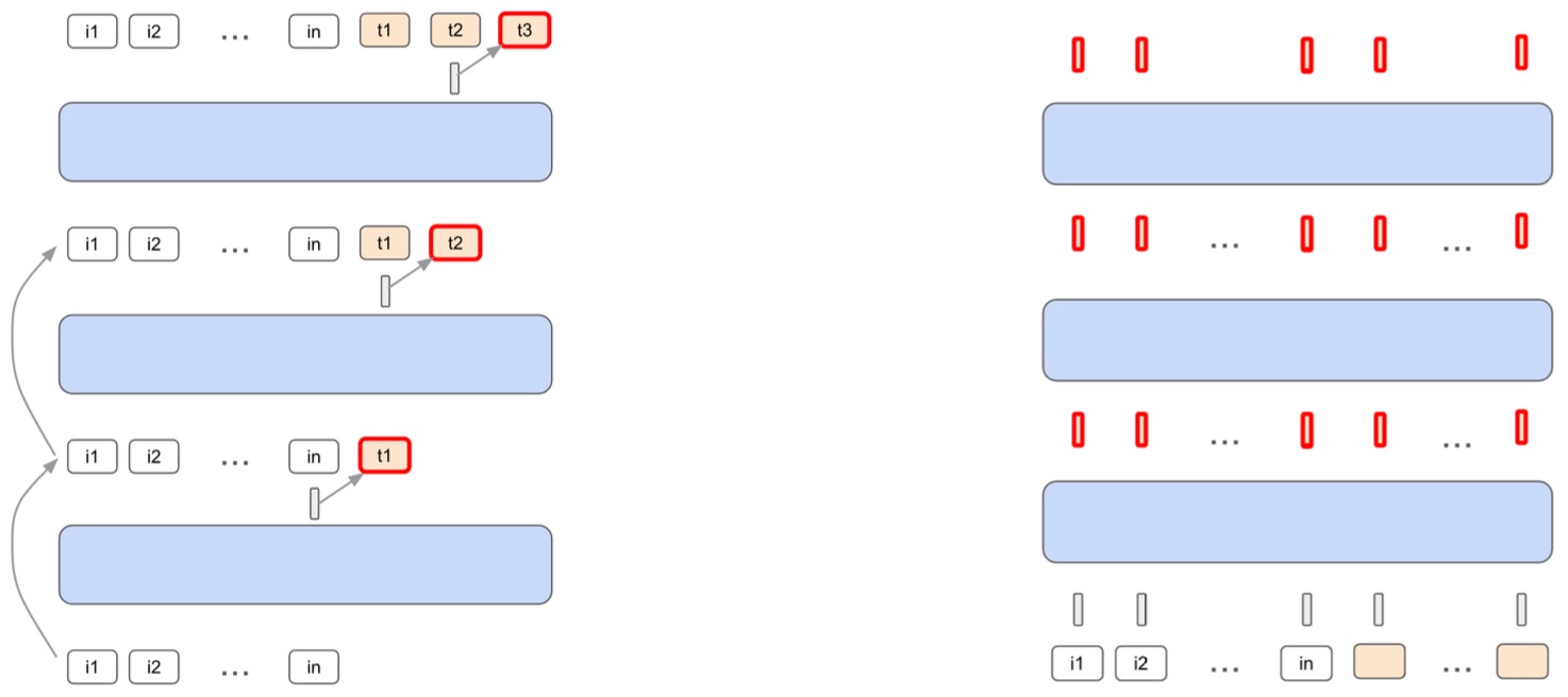
- Scaling up Test-Time Compute with Latent Reasoning by Geiping et al. (2025) demonstrates that these latent thoughts can be scaled at inference time by simply increasing the recurrence count, yielding substantial gains on mathematical and commonsense reasoning benchmarks.
Continuous Thought
-
The broader idea that reasoning need not be expressed in language is explored in Training Large Language Models to Reason in a Continuous Latent Space by Hao et al. (2025), which introduces Chain of Continuous Thought (Coconut). Instead of decoding an intermediate token, Coconut feeds the final hidden state back into the model as the next input embedding, allowing the model to reason directly in continuous space.
-
Although Coconut does not use parameter tying in the same way as looped transformers, it reinforces the same conceptual claim: the most efficient reasoning process may be one that never leaves latent space.
Implicit Composition
-
Modern language models already store vast amounts of factual knowledge in their parameters, but they often struggle to combine that knowledge in novel ways. Looped transformers appear especially effective at this composition problem because repeated applications of the same block act like iterative retrieval and synthesis.
-
Loop, Think, & Generalize: Implicit Reasoning in Recurrent-Depth Transformers by Kohli et al. (2026) studies implicit multi-hop reasoning, where models must answer questions in a single forward pass without explicit chain-of-thought. The authors show that recurrent-depth transformers can systematically combine facts that were never observed together during training, while standard transformers frequently fail.
-
For example, a model may retrieve:
- “The performer of Imagine is John Lennon.”
- “The spouse of John Lennon is Yoko Ono.”
-
By iteratively refining the hidden state, the model composes these facts internally and predicts the final answer without ever verbalizing the intermediate steps.
Systematic Generalization
-
Systematic generalization refers to the ability to recombine learned rules and facts in previously unseen configurations. In looped transformers, this capability emerges because each recurrent step applies the same transformation, encouraging the model to reuse a common reasoning procedure rather than memorize depth-specific templates.
-
Loop, Think, & Generalize: Implicit Reasoning in Recurrent-Depth Transformers by Kohli et al. (2026) shows that out-of-distribution performance emerges through a three-stage grokking process. Models first memorize training examples, then generalize within the training distribution, and finally exhibit a sudden jump in systematic generalization to unseen compositions.
-
This result suggests that recurrence encourages the emergence of reusable computational rules rather than isolated associations.
Depth Extrapolation
-
Depth extrapolation is the ability to solve problems requiring more reasoning steps than were encountered during training. Because looped transformers can execute the same block arbitrarily many times, they naturally support this form of generalization.
-
If a model is trained with recurrence depth (L_{\text{train}}), then inference can use:
-
Loop, Think, & Generalize: Implicit Reasoning in Recurrent-Depth Transformers by Kohli et al. (2026) reports that models trained on 20-hop reasoning tasks can generalize successfully to 30-hop questions by increasing recurrence depth at inference time.
-
This property is rare in conventional transformers, whose fixed architectural depth constrains the number of implicit reasoning steps available within a single forward pass.
Search Dynamics
-
Repeated refinement enables hidden states to represent multiple competing hypotheses before converging toward a final answer. Training Large Language Models to Reason in a Continuous Latent Space by Hao et al. (2025) argues that continuous latent states can encode several alternative reasoning branches simultaneously, effectively supporting breadth-first search in latent space.
-
In looped transformers, a similar phenomenon can occur when early iterations maintain uncertainty and later iterations progressively sharpen the representation. This makes recurrence analogous to iterative search, where each loop narrows the set of plausible solutions.
Reasoning and Memorization
-
A recurring theme across looped transformer research is the distinction between storing knowledge and manipulating knowledge. Parameters determine what information is encoded, while recurrence determines how deeply that information can be combined.
-
Scaling Latent Reasoning via Looped Language Models by Zhu et al. (2025) provides controlled experiments showing that looped models do not primarily benefit from larger knowledge capacity. Instead, they gain from stronger knowledge manipulation, producing reasoning traces that align more closely with correct final answers than conventional chain-of-thought.
Inference-Time Thinking
-
One of the most practical consequences of latent reasoning is that computation can be scaled at inference without retraining. For difficult questions, the model can simply run more recurrent steps, devoting additional computation to internal reasoning before generating the next token.
-
Scaling up Test-Time Compute with Latent Reasoning by Geiping et al. (2025) shows that more recurrence can dramatically improve performance, especially on tasks such as GSM8K that require substantial multi-step reasoning.
Conceptual Shift
-
Looped transformers suggest a different model of intelligence. Instead of viewing a language model as a static function that maps prompts directly to outputs, they frame it as an iterative computational process that repeatedly transforms an internal state until sufficient reasoning has occurred.
-
In this view, each recurrent step is analogous to one cycle of thought. Knowledge remains encoded in the parameters, but reasoning emerges from the repeated application of a learned computational operator. This turns inference into a controllable thinking process, where additional compute corresponds directly to additional latent reasoning depth.
Chain-of-Thought Monitorability
Architecture and monitorability are different properties
-
A recurrent-depth or looped Transformer does not inherently remove chain-of-thought. Recurrence changes how much computation can occur between emitted tokens, while chain-of-thought is an output behavior determined by training and inference. A recurrent model can perform many latent refinement steps and still generate an explicit reasoning trace afterward.
-
If a recurrent core contains \(k\) layers and executes \(R\) times before the next output token, its hidden computational depth is approximately:
\[D_{\text{hidden}} = kR\]- while the number of explicit reasoning tokens may remain unchanged. The architectural consequence is therefore additional latent sequential computation, not automatic suppression of textual reasoning.
-
A useful decomposition is:
\[C_{\text{total}} = C_{\text{latent}} + C_{\text{text}}\]- where \(C_{\text{latent}}\) is computation performed inside hidden representations and \(C_{\text{text}}\) is computation obtained by autoregressively producing additional reasoning tokens. Increasing recurrent depth directly increases the capacity of \(C_{\text{latent}}\), but it does not mathematically require \(C_{\text{text}}\) to decrease.
-
Scaling up Test-Time Compute with Latent Reasoning: A Recurrent Depth Approach by Geiping et al. (2025) demonstrates that recurrent blocks can substantially increase test-time reasoning computation without generating additional chain-of-thought tokens, establishing latent recurrence as an alternative computation channel rather than a mechanism for disabling explicit reasoning.
Why recurrent depth changes the monitorability question
-
The safety significance comes from where sequential computation can occur. In an ordinary reasoning model, one way to obtain substantially more sequential reasoning is to generate more intermediate tokens:
\[x \rightarrow r_1 \rightarrow r_2 \rightarrow \cdots \rightarrow r_T \rightarrow y\]- where the reasoning tokens \(r_1,\ldots,r_T\) can potentially be inspected by a monitor.
-
A recurrent-depth model adds another path:
\[x \rightarrow h^{(1)} \rightarrow h^{(2)} \rightarrow \cdots \rightarrow h^{(R)} \rightarrow y\]- where \(h^{(r)}\) is a continuous hidden representation rather than a natural-language statement.
-
Reasoning with Latent Thoughts: On the Power of Looped Transformers by Saunshi et al. (2025) gives a theoretical connection between these two forms of computation, showing that looped Transformers can simulate multi-step chain-of-thought-style computations through repeated latent updates.
-
The distinction is therefore not:
\[\text{looped model} \Rightarrow \text{no chain-of-thought}\]-
but rather:
\[\text{looped model} \Rightarrow \text{more sequential computation can occur without chain-of-thought}\]
-
-
This distinction matters because a safety monitor cannot directly read ordinary residual-stream activations in the same way it can read natural-language reasoning. If capability increasingly comes from \(C_{\text{latent}}\) while the observable textual trace remains short, chain-of-thought may capture a smaller fraction of the computation relevant to the final behavior.
What chain-of-thought monitorability measures
-
Chain of Thought Monitorability: A New and Fragile Opportunity for AI Safety by Korbak et al. (2025) frames natural-language reasoning as a potentially valuable safety signal because monitors can inspect a model’s reasoning for indications of deception, reward hacking, policy circumvention, or other undesirable intent, while emphasizing that this form of oversight is imperfect and potentially fragile.
-
Monitorability can be abstracted as follows. Let \(z\) denote some property of an agent’s behavior that an overseer wants to detect, let \(o\) denote the observations available to a monitor, and let \(m(o)\) be the monitor’s prediction. A generic monitorability score can be written as:
\[M = \mathbb{E} \left[ S \left( m(o),z \right) \right]\]- where \(S\) is an appropriate classification or prediction score.
-
Crucially, the observation \(o\) can contain different information:
-
Monitoring Monitorability by Guan et al. (2025) operationalizes this idea through intervention, process, and outcome-property evaluations and finds that access to chain-of-thought generally makes monitors substantially more informative than observing actions and final outputs alone.
-
Evaluating chain-of-thought monitorability similarly reports a suite of \(13\) evaluations spanning \(24\) environments, designed to measure whether monitors can infer properties of an agent’s reasoning and behavior from different observation channels. ([OpenAI][5])
Longer reasoning traces can improve monitorability
-
A central empirical finding of Monitoring Monitorability by Guan et al. (2025) is that longer chains-of-thought tend to be more monitorable. More textual reasoning provides the monitor with additional evidence about intermediate goals, assumptions, strategies, and deviations from intended behavior.
-
This creates a potential tension with latent test-time scaling. Suppose two equally capable systems allocate their reasoning budgets differently:
\[C_{\text{total}}^{(A)} = C_{\text{latent}}^{(A)} + C_{\text{text}}^{(A)}\] \[C_{\text{total}}^{(B)} = C_{\text{latent}}^{(B)} + C_{\text{text}}^{(B)}\]- with \(C_{\text{latent}}^{(A)}>C_{\text{latent}}^{(B)}\) and \(C_{\text{text}}^{(A)}<C_{\text{text}}^{(B)}\).
-
Even if the systems have similar total inference compute and capability, system \(A\) may expose less textual evidence to a chain-of-thought monitor. This is the meaningful monitorability concern associated with latent reasoning. It is a substitution effect between forms of computation, not an intrinsic property of parameter sharing.
-
Monitoring Monitorability by Guan et al. (2025) additionally find an interesting capability-matched trade-off: in some settings, a smaller model running at higher explicit reasoning effort can reach capability comparable to a larger model operating at lower reasoning effort while remaining more monitorable, although it pays greater inference compute. Guan et al. refers to this additional cost as a monitorability tax.
Hidden computation already exists in ordinary Transformers
- Recurrent depth does not introduce latent computation from nothing. Every standard Transformer already performs many hidden attention and MLP transformations before producing a token:
-
None of the intermediate states \(h_1,\ldots,h_D\) is intrinsically human-readable. A chain-of-thought trace is therefore already an externalized reasoning channel layered on top of substantial latent neural computation.
-
Recurrent depth changes the scale of that channel. If a \(D\)-layer model reuses its layers \(R\) times, the model obtains approximately \(DR\) sequential hidden transformations between emitted tokens rather than \(D\).
-
Consequently, the relevant safety question is not whether recurrent Transformers have hidden reasoning while ordinary Transformers do not. Both do. The relevant question is whether increasing latent computational depth causes more decision-relevant reasoning to migrate away from observable textual traces.
Chain-of-thought monitorability is not the same as faithfulness
-
Even a fully visible chain-of-thought is not necessarily a faithful causal account of how a model reached its answer. A model can produce a plausible explanation that omits factors that actually influenced its decision.
-
Measuring Faithfulness in Chain-of-Thought Reasoning by Lanham et al. (2023) tests faithfulness by intervening on reasoning traces, including truncating, paraphrasing, and perturbing intermediate reasoning, and finds substantial variation in how strongly model predictions actually depend on the stated chain-of-thought.
-
Monitorability and faithfulness should therefore be separated:
-
Visibility asks whether reasoning text exists. Faithfulness asks whether that text reflects the causal computation producing the answer. Monitorability asks whether an observer can use the available trace to infer properties of the model’s behavior.
-
A long but post-hoc rationalization can be highly visible yet poorly faithful. Conversely, a partially faithful trace may still be useful for detecting undesirable intentions. Chain-of-thought monitoring should therefore be treated as an empirical oversight mechanism, not as guaranteed access to the model’s complete internal computation.
Latent reasoning need not be uninterpretable by construction
-
Hidden-state reasoning is harder to inspect directly than natural-language reasoning, but recurrent depth does not imply that latent representations are fundamentally uninterpretable.
-
Bridging the Gap Between Latent and Explicit Reasoning with Looped Transformers by Fan et al. (2026) introduces LOTUS, which supervises latent positions against corresponding explicit chain-of-thought steps while performing recurrent computation in parallel latent blocks. At \(3\)B parameters, the method matches explicit-CoT reasoning in its studied setting while reducing thought-phase latency by approximately \(2.5\times\) to \(6.9\times\).
-
More importantly for interpretability, projecting LOTUS’s post-loop latent states through the language-model head recovers the corresponding reasoning steps and sometimes reveals alternative valid intermediate steps. Bridging the Gap Between Latent and Explicit Reasoning with Looped Transformers by Fan et al. (2026) therefore demonstrates that latent reasoning can be deliberately trained to remain aligned with interpretable textual concepts.
-
This suggests another design axis:
\[\text{latent reasoning} + \text{interpretability supervision}\]- rather than treating efficient hidden computation and inspectability as necessarily mutually exclusive.
Recurrent depth does not by itself explain current monitorability regressions
-
The distinction is especially important when interpreting recent frontier-model results. Safety overview: GPT-6 Astra reports that Astra shows a substantial decrease in chain-of-thought monitorability relative to earlier models and an increased ability to evade monitors under adversarial evaluation. It also reports increased control over the model’s own chain-of-thought. ([OpenAI][8])
-
These observations do not establish that recurrent depth is the cause. The public Astra safety analysis evaluates the behavior of the complete trained system rather than an architecture-controlled ablation in which recurrence is the only changed variable.
-
An Alien Mind identifies several broader forces that can weaken reliance on chain-of-thought monitoring: models operate in increasingly complex environments where reasoning is interleaved with tools and communication, stronger systems can reason about and manipulate their own reasoning process, and improved pretraining allows increasingly capable behavior even without extensive verbalized reasoning.
-
This means the causal claim:
\[\text{recurrent depth} \Rightarrow \text{lower CoT monitorability}\]- is substantially stronger than the presently established evidence.
-
The evidence instead supports the weaker and more defensible relationship:
\[\text{more capable latent computation} \Rightarrow \text{potentially less dependence on explicit CoT}\]- and reduced dependence on explicit CoT can, under some training and inference regimes, reduce the information available to a textual monitor.
How to test whether recurrence causes a monitorability loss
-
Isolating the architectural effect requires capability-controlled experiments. A meaningful comparison should train recurrent and non-recurrent models with matched data, objectives, post-training procedures, and approximately matched downstream capability.
-
At minimum, such an evaluation should vary recurrence \(R\) while measuring:
- A useful experimental matrix would compare:
| Model | Effective depth | Explicit CoT budget | Capability | Monitorability |
|---|---|---|---|---|
| Standard Transformer | fixed | fixed | measured | measured |
| Deeper Transformer | increased | fixed | matched | measured |
| Looped Transformer | increased by recurrence | fixed | matched | measured |
| Looped Transformer + longer CoT | increased by recurrence | increased | matched | measured |
- Comparing a looped model only with a smaller or weaker non-looped baseline cannot distinguish an architectural monitorability effect from capability, reasoning-effort, or output-length effects. Monitoring Monitorability by Guan et al. (2025) demonstrates why these controls matter by showing that model size, reasoning effort, available monitor compute, and CoT length can all affect measured monitorability.
Monitoring beyond natural-language reasoning
-
If increasingly capable models move useful computation into latent states, oversight does not have to be restricted to either chain-of-thought or final actions. A richer monitoring stack can combine several channels:
- textual chain-of-thought;
- tool calls and environment actions;
- final outputs;
- recurrent-depth activation probes;
- latent-to-text decoders;
- anomaly detectors over hidden states;
- follow-up elicitation designed to expose otherwise implicit reasoning.
-
Monitoring Monitorability by Guan et al. (2025) finds that asking agents follow-up questions and exposing the resulting chain-of-thought to the monitor can improve monitorability, suggesting that reasoning traces need not be treated as a single immutable artifact generated during the original trajectory.
-
An Alien Mind similarly motivates combining chain-of-thought monitoring with activation-level monitoring as models become less dependent on verbalized reasoning.
Takeaway
-
Recurrent depth increases the amount of computation that can occur inside continuous hidden states before the model emits text. That makes latent computation a stronger substitute for explicit chain-of-thought, which is relevant to safety because natural-language reasoning currently provides a useful monitoring signal.
-
It does not follow that looped Transformers inherently hide their reasoning, eliminate chain-of-thought, or are necessarily less monitorable than equally capable non-looped models. The architecture creates the capacity for more unobserved computation; whether that capacity reduces practical monitorability depends on training, reasoning policy, output length, latent-state structure, and the monitoring methods available.
-
The central research objective is therefore not to prevent latent reasoning, but to preserve useful observability as reasoning increasingly spans both textual and continuous representations.
Generalization
- A defining feature of looped transformers is that they improve not only raw benchmark performance but also the ability to generalize beyond the exact patterns seen during training. Conventional transformers often store large amounts of knowledge yet struggle to recombine that knowledge compositionally or to solve tasks requiring deeper reasoning chains than were represented in the training distribution. By repeatedly applying the same transformation, looped transformers encourage the emergence of reusable computational procedures that can be deployed in novel settings.
Systematic Composition
-
Systematic generalization refers to the ability to combine known facts, rules, or operators in previously unseen ways. In a standard transformer, different layers specialize to different representational roles, and the model may memorize shallow associations rather than learn a reusable reasoning mechanism. In a looped transformer, every recurrent step applies the same block, forcing the model to reuse a common update rule across all stages of reasoning.
-
Loop, Think, & Generalize: Implicit Reasoning in Recurrent-Depth Transformers by Kohli et al. (2026) demonstrates that recurrent-depth transformers can solve out-of-distribution multi-hop tasks where models must compose facts that were never combined during training.
-
If the hidden state contains a partial reasoning result (h_t), each recurrent application can be viewed as a composition operator:
- Because the same operator is reused, the model learns a general transformation rather than a depth-specific lookup table.
Depth Extrapolation
-
Depth extrapolation is the ability to solve problems requiring more reasoning steps than were encountered during training. This is one of the most striking properties of looped transformers.
-
Suppose a model is trained on problems requiring up to \(k\) latent reasoning steps. At inference, the same recurrent block can be applied for more than \(k\) iterations:
-
If the recurrent operator implements a stable reasoning procedure, the model can continue composing information beyond its training horizon.
-
Loop, Think, & Generalize: Implicit Reasoning in Recurrent-Depth Transformers by Kohli et al. (2026) shows that models trained on 20-hop reasoning can successfully answer 30-hop questions by simply increasing recurrence depth at test time.
-
This property closely resembles how an algorithm trained to perform one iteration of an update rule can be run repeatedly until convergence.
Grokking Dynamics
-
Systematic generalization in looped transformers often emerges abruptly rather than gradually. During training, the model first memorizes the training set, then generalizes within the training distribution, and finally undergoes a sharp transition to strong out-of-distribution performance.
-
The following figure (source) shows recurrent-depth model accuracy curves across training epochs and wall-clock time, illustrating the emergence of systematic generalization through training. The left panel plots test OOD accuracy for models trained with \(R \in {1,2,4,8}\) against training epochs, with curves smoothed by a 100-epoch rolling mean and shading indicating standard deviation. The middle panel plots test OOD accuracy for the same models against training wall-clock time in hours. The right panel focuses on the \(R=4\) model and compares accuracy on training, ID test, and OOD test examples across training epochs.
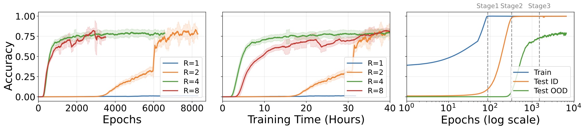
-
Loop, Think, & Generalize: Implicit Reasoning in Recurrent-Depth Transformers by Kohli et al. (2026) identifies this as a three-stage grokking process, supported by mechanistic analysis of how internal representations evolve.
-
This behavior suggests that the recurrent block eventually discovers a compact algorithmic rule that can be applied repeatedly rather than relying on memorized templates.
Algorithmic Transfer
-
Looped transformers are naturally aligned with algorithmic tasks because iterative algorithms already consist of repeated applications of a common update rule. Once the model learns this update, it can transfer the procedure to larger or more complex instances.
-
Looped Transformers Are Better at Learning Learning Algorithms by Yang et al. (2024) shows that looped models excel at in-context regression and other tasks where the optimal solution is iterative, effectively internalizing learning algorithms with a small number of shared parameters.
-
Looped Transformers as Programmable Computers by Giannou et al. (2023) extends this argument by demonstrating that looped transformers can emulate function calls, conditional branches, and memory manipulation, enabling general-purpose computation.
Knowledge Composition
-
Modern language models often contain the facts needed to answer complex questions but fail to chain those facts together. Looped transformers improve this by repeatedly retrieving, transforming, and integrating parametric knowledge.
-
Scaling Latent Reasoning via Looped Language Models by Zhu et al. (2025) provides controlled experiments showing that looped models outperform much larger baselines primarily through superior knowledge manipulation rather than increased memorization.
-
This result reinforces the idea that generalization depends critically on the model’s ability to iteratively compose stored information.
Overthinking Limits
-
Generalization is not unbounded. If the recurrent operator is applied too many times, the hidden state may drift away from the correct solution, causing accuracy to decline \(\text{Acc}(L+1) < \text{Acc}(L)\) for sufficiently large \(L\).
-
This phenomenon, often called overthinking, places a practical limit on how far recurrence can be extended without additional safeguards. Loop, Think, & Generalize: Implicit Reasoning in Recurrent-Depth Transformers by Kohli et al. (2026) identifies overthinking as a central limitation when extrapolating far beyond the training regime.
Generalization View
-
The broader lesson is that looped transformers transform depth from a fixed architectural constant into a reusable computational process. Because the same transformation is applied repeatedly, the model is encouraged to learn general-purpose reasoning procedures rather than collections of specialized layer behaviors.
-
This leads to two unusually strong forms of extrapolation: systematic composition, where the model recombines knowledge in new ways, and depth extrapolation, where it continues reasoning beyond the depths seen during training. Together, these properties suggest that recurrence is not merely a parameter-sharing trick but a mechanism for inducing more algorithmic and compositional forms of intelligence.
Test-Time Compute
- One of the most consequential properties of looped transformers is that they can consume more computation at inference time without changing their parameters. This makes reasoning depth a runtime decision rather than a fixed architectural constant. A model can therefore devote additional internal computation to difficult problems simply by executing more recurrent iterations before predicting the next token.
Runtime Depth
-
In a conventional transformer, the number of sequential transformations is fixed by the architecture. A 48-layer model always performs 48 layers of computation per token. In a looped transformer, the recurrent block can be executed for any number of iterations:
\[h_{t+1} =f_\theta(h_t,x) \quad t = 0,\dots,L-1\]- where \(L\) is selected at inference time. Increasing \(L\) increases effective depth and computational cost while leaving parameter count unchanged.
-
Scaling up Test-Time Compute with Latent Reasoning by Geiping et al. (2025) demonstrates that a recurrent-depth language model can continue improving on reasoning benchmarks as recurrence depth is increased far beyond its nominal parameter size.
Latent Scaling
-
The core intuition is that the model “thinks longer” internally rather than generating longer intermediate text. Each additional iteration refines the hidden state, allowing more retrieval, composition, and search to occur before the output is produced.
-
The following figure shows how benchmark accuracy increases as recurrence depth grows.
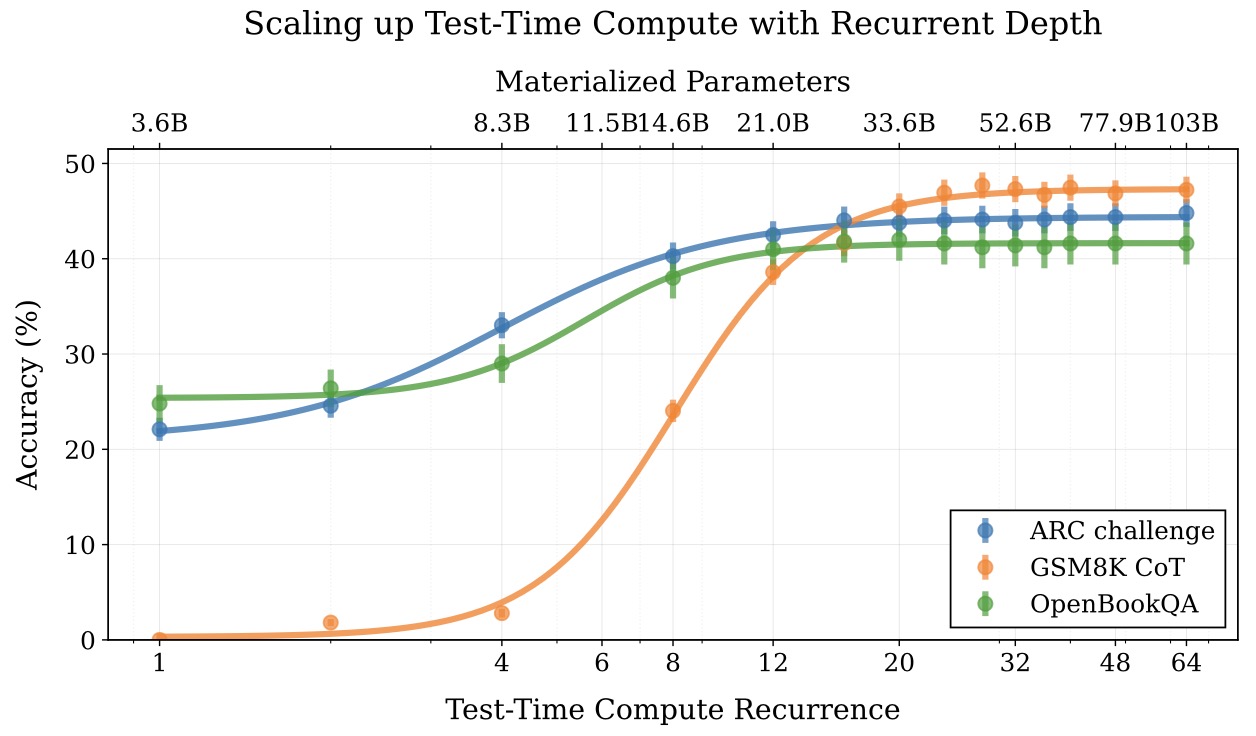
- In Scaling up Test-Time Compute with Latent Reasoning by Geiping et al. (2025), a 3.5B recurrent-depth model reaches a computational footprint equivalent to tens of billions of effective parameters when recurrence is increased at inference time, with especially large gains on arithmetic and multi-step reasoning tasks.
Performance Curves
-
Performance usually improves with additional loops before approaching a plateau. A common empirical model is:
\[\epsilon(L) \approx \epsilon_\infty + A e^{-kL}\]- where \(\epsilon(L)\) is the error after \(L\) loops, \(\epsilon_\infty\) is the asymptotic error, and \(A e^{-kL}\) captures diminishing returns.
-
Parcae: Scaling Laws for Stable Looped Language Models by Prairie et al. (2026) shows that this saturating behavior is highly predictable, making recurrence depth a controllable and quantifiable source of additional capability.
Adaptive Depth
-
The most powerful use of test-time compute is not to apply the same number of loops to every example, but to allocate computation dynamically based on problem difficulty.
-
If an exit mechanism estimates the probability that the current state is sufficient, computation can stop once a confidence threshold is reached:
\[\text{stop if } p_{\text{exit}}(h_t) > \tau\]- where \(\tau\) is a predetermined threshold.
-
Scaling Latent Reasoning via Looped Language Models by Zhu et al. (2025) incorporates an exit gate that allows simple examples to terminate after fewer loops while reserving deeper recurrence for harder inputs.
Token Routing
-
Some architectures refine adaptive depth further by allowing different tokens in the same sequence to receive different amounts of recurrent computation.
-
Mixture-of-Recursions: Learning Dynamic Recursive Depths for Adaptive Token-Level Computation by Bae et al. (2025) introduces lightweight routers that determine which tokens continue to participate in each recursion step. Tokens that have already converged are skipped, reducing both attention cost and key-value cache requirements.
-
This creates a token-specific depth function:
\[L_i =g(x_i)\]- where \(L_i\) is the number of recursions allocated to token \(i\).
-
The following figure (source) shows an overview of Mixture-of-Recursions (MoR). The left panel shows a recursion step made of a fixed stack of layers and a router that decides whether each token should continue through the block or exit. The middle panel shows the full model structure, where the shared recursion step is applied up to \(N_r\) times for each token depending on the router decision. The right panel shows an example token-wise routing pattern, where dark blue cells indicate active computation, light gray cells indicate skipped computation, and the colored labels below the sequence indicate whether each subword token uses \(1\), \(2\), or \(3\) recursion steps, shown as pink for \(1\), light blue for \(2\), and peach for \(3\), to predict the next token.
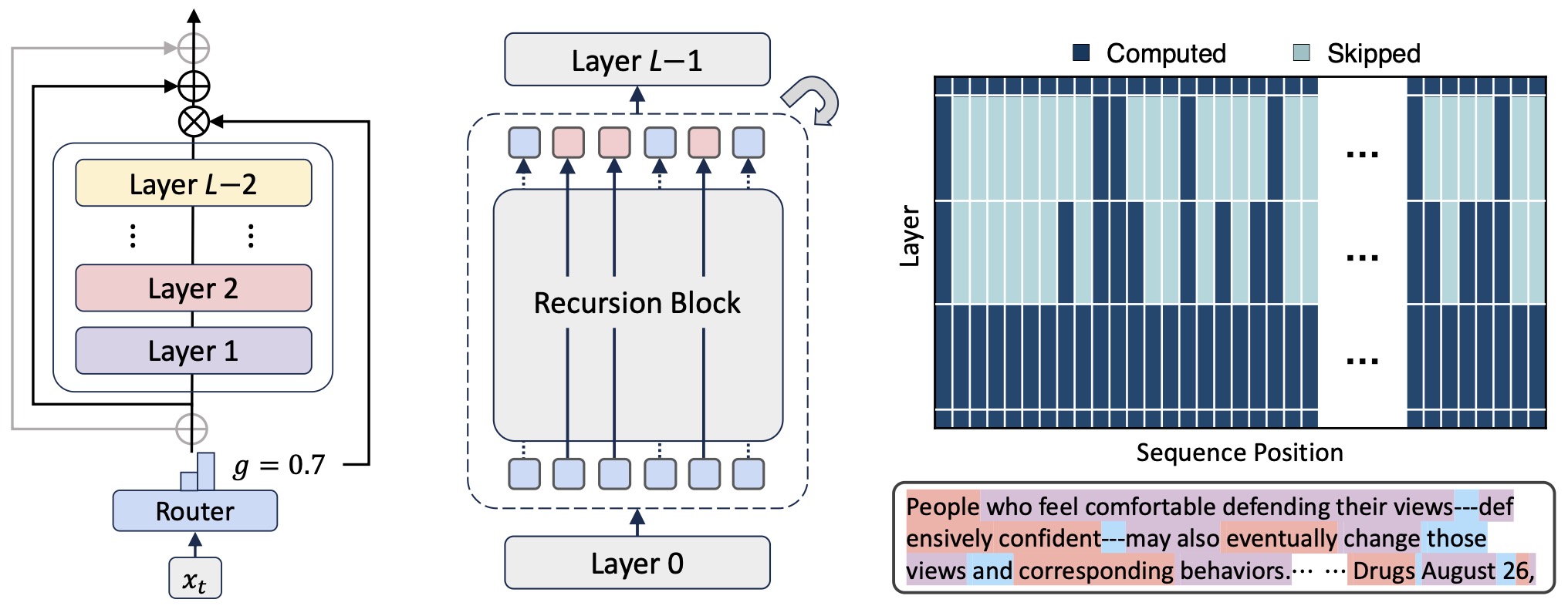
Latency Tradeoffs
-
Because parameter memory remains fixed, looped transformers convert memory costs into latency costs. Running more loops increases sequential computation and wall-clock time, but avoids storing a much larger model.
-
This introduces a flexible deployment trade-off. A system can:
- Use fewer loops for low-latency applications.
- Increase loops for difficult reasoning tasks.
- Terminate early when confidence is high.
- Scale computation according to available hardware budget.
-
The resulting model behaves similarly to an anytime algorithm, producing progressively better internal states as more compute becomes available.
Training Mismatch
-
To benefit from test-time scaling, the model must be trained so that additional loops remain productive. If the recurrent operator is optimized only for a fixed depth, increasing recurrence at inference may cause overthinking or instability.
-
Common strategies include stochastic depth sampling, multi-step supervision, and curricula over loop count. These techniques ensure that each additional iteration tends to refine rather than degrade the hidden state.
-
Loop, Think, & Generalize: Implicit Reasoning in Recurrent-Depth Transformers by Kohli et al. (2026) shows that training choices strongly affect how well recurrent-depth transformers extrapolate to deeper reasoning chains.
Compute Economics
-
Test-time recurrence fundamentally changes the economics of scaling. Instead of deploying a larger model for all requests, one can deploy a compact looped model and selectively allocate more computation only when needed.
-
If model capability is viewed as a function of parameters \(N\) and inference compute \(C_{\text{test}}\),
\[\text{Capability} =f(N, C_{\text{test}})\]- then looped transformers expose \(C_{\text{test}}\) as a first-class control variable. This allows a single model to operate across a wide range of latency and quality targets, from fast responses with minimal recurrence to deep latent reasoning with substantially larger compute budgets.
-
In practical terms, looped transformers transform inference from a fixed-cost operation into an adaptive thinking process whose depth can be tuned continuously according to the complexity of the problem.
Universal Transformers: Recurrent Self-Attention over Depth
Core idea
-
Universal Transformers by Dehghani et al. (2018) introduced one of the earliest transformer architectures in which computation is recurrent over depth: instead of applying a fixed sequence of independently parameterized transformer layers, the model repeatedly applies a shared self-attention and transition function to progressively refine the representation at every sequence position.
-
The key distinction is that recurrence occurs over successive revisions of hidden representations rather than over sequence positions. A conventional recurrent neural network progresses sequentially from one token to the next, whereas the Universal Transformer updates all sequence positions in parallel at each recurrent step and then repeats this global refinement procedure. This preserves much of the parallelism and global receptive field introduced by Attention Is All You Need by Vaswani et al. (2017), while restoring an iterative-computation inductive bias analogous to recurrent networks.
-
This creates an important separation between parameter count and computational depth. With a fixed number of recurrent steps, a Universal Transformer is effectively a deep Transformer whose self-attention and transition parameters are tied across depth. Increasing the number of recurrent steps therefore increases effective computational depth without introducing a distinct parameter set for every additional layer.
The following figure (source) shows how the Universal Transformer repeatedly refines the vector representation at every sequence position in parallel, using self-attention to exchange information among positions and a shared transition function to update each position across recurrent depth steps.
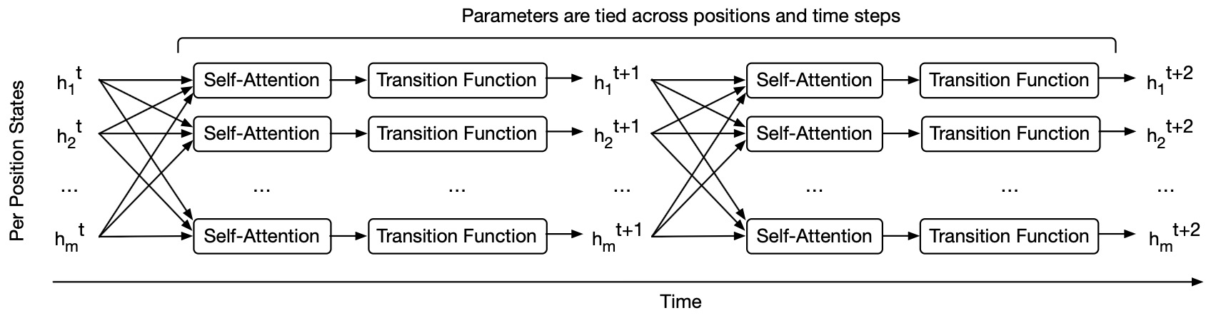
Recurrent refinement
-
Given a sequence of token representations, each recurrent step first performs multi-head self-attention over the complete sequence and then applies a position-wise transition function. Universal Transformers by Dehghani et al. (2018) uses the same learned transformation parameters across recurrent steps, so recurrence changes the hidden state while the operator performing that update remains shared.
-
The underlying scaled dot-product attention remains the standard Transformer operation:
- At recurrent step \(t\), self-attention first produces an intermediate representation:
- The shared transition function then performs the recurrent state update:
-
The transition may be a position-wise feed-forward network or a depth-wise separable convolution. Residual connections and layer normalization surround the attention and transition operations, analogous to the original Transformer architecture.
-
Because the same transformation is executed repeatedly, the model must distinguish both where a token occurs in the sequence and which recurrent refinement step is currently being executed. Universal Transformers therefore combine ordinary positional information with a recurrent-step encoding. For position \(i\), recurrent step \(t\), and representation dimension \(j\), the sinusoidal coordinates are constructed as:
- The additional depth coordinate is important because otherwise identical shared weights would have no explicit signal indicating whether they are being applied during an early representation-building step or a later refinement step.
Dynamic per-position computation
-
A particularly important contribution of Universal Transformers by Dehghani et al. (2018) is that recurrence need not be uniformly fixed. The architecture incorporates Adaptive Computation Time for Recurrent Neural Networks by Graves (2016), allowing different sequence positions to receive different numbers of recurrent updates according to learned halting probabilities.
-
Conceptually, a small halting head computes a probability after each recurrent state:
- Computation for position \(i\) can terminate once accumulated halting probability reaches a threshold:
-
Positions that have already halted no longer require additional state transformations. Their state is propagated forward while unresolved positions continue through further recurrent steps, until all positions halt or a predefined maximum depth is reached. This creates per-position conditional computation rather than merely applying a globally fixed number of repeated layers.
-
This mechanism is a direct conceptual ancestor of modern adaptive recurrent-depth architectures. Mixture-of-Recursions: Learning Dynamic Recursive Depths for Adaptive Token-Level Computation by Bae et al. (2025), for example, replaces ACT-style halting with explicit routers that allocate different recursion depths to different tokens while reusing a shared layer stack.
Adaptive depth as learned reasoning effort
-
The Universal Transformer experiments provide early evidence that learned recurrent depth can correlate with problem complexity rather than behaving as arbitrary additional computation. On bAbI tasks requiring one, two, and three supporting facts, average ponder time increased from approximately \(2.3\pm0.8\) steps to \(3.1\pm1.1\) and \(3.8\pm2.2\) steps respectively.
-
More importantly, computation was non-uniform within individual examples. In tasks containing many irrelevant facts, numerous positions halted after only one or two recurrent steps, while a smaller set of positions continued receiving additional processing. Attention also became progressively sharper around relevant supporting facts over successive recurrent steps, making the recurrent trajectory resemble an iterative multi-hop memory-access procedure.
The following figure (source) shows the learned ponder time of a Universal Transformer with dynamic halting on a bAbI example requiring three supporting facts, illustrating that different facts and question positions receive substantially different amounts of recurrent computation.
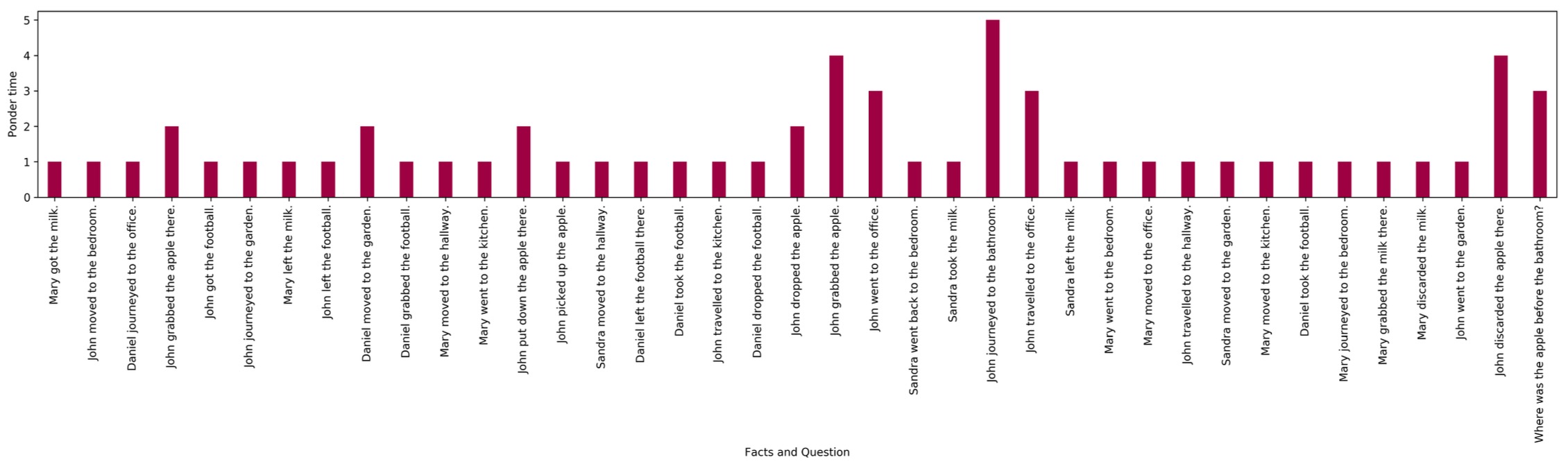
Encoder-decoder formulation
-
The original Universal Transformer is an encoder-decoder model rather than the decoder-only architecture common in contemporary LLMs. The encoder repeatedly refines all source positions with a recurrent self-attention block. The decoder has the same recurrent structure, but additionally performs encoder-decoder attention to the final source representations before applying its transition function.
-
The following figure (source) shows the Universal Transformer encoder-decoder architecture. Both the encoder and decoder repeatedly apply shared recurrent blocks for \(T\) steps: the encoder alternates multi-head self-attention with a transition function, while the decoder additionally performs multi-head attention over the final encoder representation before producing output probabilities through a softmax layer. With dynamic halting, the number of recurrent steps \(T\) can be determined independently for each sequence position using Adaptive Computation Time.
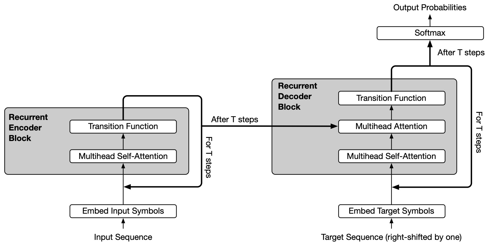
- After recurrent refinement, the decoder maps its final hidden state to the vocabulary and predicts tokens autoregressively:
- For standard sequence generation, training therefore retains the familiar teacher-forced negative log-likelihood objective:
- The architectural novelty is therefore not a fundamentally different token-level prediction objective. It is the computational graph used to construct the representation from which that prediction is made: the hidden state can undergo repeated, parameter-shared refinement before being decoded.
Empirical behavior
-
The strongest early results appeared on tasks requiring iterative or algorithmic computation. On the 10K-example single-task bAbI setting, the standard Transformer reported an average error of \(15.2\) with \(10\) of \(20\) tasks failing the specified error threshold, whereas the fixed-depth Universal Transformer achieved \(0.23\) average error with no failed tasks, and the dynamically halted variant achieved \(0.21\) with no failed tasks.
-
The architecture also generalized substantially better on synthetic algorithmic tasks. When trained on copy, reverse, and addition sequences of length 40 and evaluated on sequences up to length 400, the Universal Transformer substantially outperformed both LSTMs and standard Transformers, consistent with the hypothesis that recurrence over depth provides an inductive bias for repeatedly applying learned algorithmic transformations.
-
On learning-to-execute tasks, Universal Transformers achieved perfect sequence accuracy on copy, double, and reverse memorization tasks and improved substantially on several program-execution tasks, again indicating that repeated transformation can be advantageous when the desired computation itself has iterative structure.
-
On LAMBADA, dynamic halting produced a test language-modeling perplexity of 142, compared with 319 for the six-step fixed Universal Transformer and \(7321\) for the Transformer baseline reported in the same experiment. Fixed eight- and nine-step Universal Transformers improved substantially over six steps, but still did not outperform dynamic halting, suggesting that the gain was not explained solely by increasing average depth.
-
Recurrence also transferred to a large-scale natural-language task. On WMT14 English-German translation, the base Universal Transformer reached 28.9 BLEU compared with 28.0 for the comparable Transformer baseline, an improvement of 0.9 BLEU with approximately the same parameter count. Importantly, the best translation configuration used fixed recurrence rather than adaptive halting, showing that conditional depth was not uniformly beneficial across tasks.
Computational universality
-
The name “Universal Transformer” refers to a theoretical property rather than merely its applicability across tasks. Under the assumptions described in Universal Transformers by Dehghani et al. (2018), a Universal Transformer with sufficient memory and a number of recurrent steps that can scale with the input can simulate a computationally universal machine.
-
The distinction from a fixed-depth Transformer is important. A conventional Transformer has a predetermined number of sequential computational transformations regardless of input complexity. A Universal Transformer can repeatedly execute the same transformation, allowing computational depth to scale independently from the number of stored parameter sets.
-
The paper establishes the connection constructively by showing that a Neural GPU can be reduced to a Universal Transformer when self-attention is configured appropriately, the transition function is convolutional, and recurrent depth scales with input length. Neural GPUs Learn Algorithms by Kaiser and Sutskever (2015) had already demonstrated a parallel recurrent architecture capable of learning algorithmic procedures and generalizing them to longer inputs.
-
Computational universality should not be interpreted as a guarantee that a trained model will discover arbitrary algorithms or generalize perfectly. Rather, it characterizes the expressive capacity made possible when attention-accessible memory is combined with recurrent computation whose depth is not architecturally fixed.
Connection to modern recurrent-depth transformers
-
Universal Transformers established three ideas that recur almost unchanged in contemporary looped models: parameter sharing across depth, iterative latent-state refinement, and adaptive computation. What has changed is primarily scale and deployment context.
-
Modern recurrent-depth language models usually apply the same principle inside decoder-only LLMs. Scaling up Test-Time Compute with Latent Reasoning: A Recurrent Depth Approach by Geiping et al. (2025) repeatedly executes a shared latent block and shows that additional recurrence at inference time can increase reasoning performance without generating additional chain-of-thought tokens.
-
Likewise, Mixture-of-Recursions: Learning Dynamic Recursive Depths for Adaptive Token-Level Computation by Bae et al. (2025) can be viewed as a modern routing-based realization of the Universal Transformer’s per-position adaptive-computation principle: shared parameters provide parameter efficiency, while token-level routing determines which representations merit additional recurrent processing.
-
In this sense, the Universal Transformer is not merely an historical precursor to looped transformers. It already contains the central architectural decomposition behind recurrent depth: a reusable learned operator, a latent state that evolves through repeated application of that operator, and an optional mechanism that decides how much computation individual positions require.
Staircase and Ladder Attention
-
Several years before looped language models became a major focus in large-scale pretraining, researchers at FAIR explored a closely related idea: increasing computation by repeatedly reusing the same transformer parameters. Their work on staircase attention and its simplified variant, ladder attention, introduced a family of recurrent attention architectures that explicitly decoupled parameter count from computation and anticipated many of the core ideas that now underpin looped transformers.
-
Staircase Attention for Recurrent Processing of Sequences by Ju et al. (2021) presents a recurrent attention mechanism that processes a sequence over multiple steps, combining recurrence over sequence positions with recurrence in depth. The accompanying FAIR article Which one is more important: more parameters or more computation? frames the broader motivation, arguing that model size and computation should be treated as distinct resources rather than inseparable aspects of a single architecture.
Staircase Processing
-
In staircase attention, computation unfolds over repeated processing steps. Each step contains two conceptual phases. A backward phase re-encodes the tokens processed so far, allowing the model to revise its understanding of prior context, and a forward phase incorporates new tokens from the input stream. This creates a staggered pattern of computation in which hidden states are refined repeatedly while new information is gradually introduced.
-
If \(h_t\) denotes the hidden state after processing step \(t\), the update can be abstractly written as:
\[h_{t+1} =f_\theta(h_t, x_{\leq t})\]- where the same parameters \(\theta\) are reused across all steps. This formulation is structurally similar to modern recurrent-depth transformers, differing mainly in how sequence progression and recurrent refinement are interleaved.
-
The following figure (source) shows staircase, ladder, and standard attention-style recurrent processing layouts, where repeated shared-weight computation trades additional compute for stronger modeling power. Specifically, the proposed staircase-family recurrent attention layouts are shown, where each outlined row is a parallel computation and rows are computed recurrently from bottom to top using shared weights. In the Staircase model, each time step introduces one new input chunk while recurrently processing a fixed number of previous chunks. In Cached Staircase, the final output state is cached and later included within the attention span after a fixed amount of recurrent processing. In Global Cached Staircase, all previous chunks are cached and attended in the final chunk. In the Ladder model, the full sequence is fed in without chunking and the same transformer computation is repeated a fixed number of times, making it the closest variant to modern looped transformers.
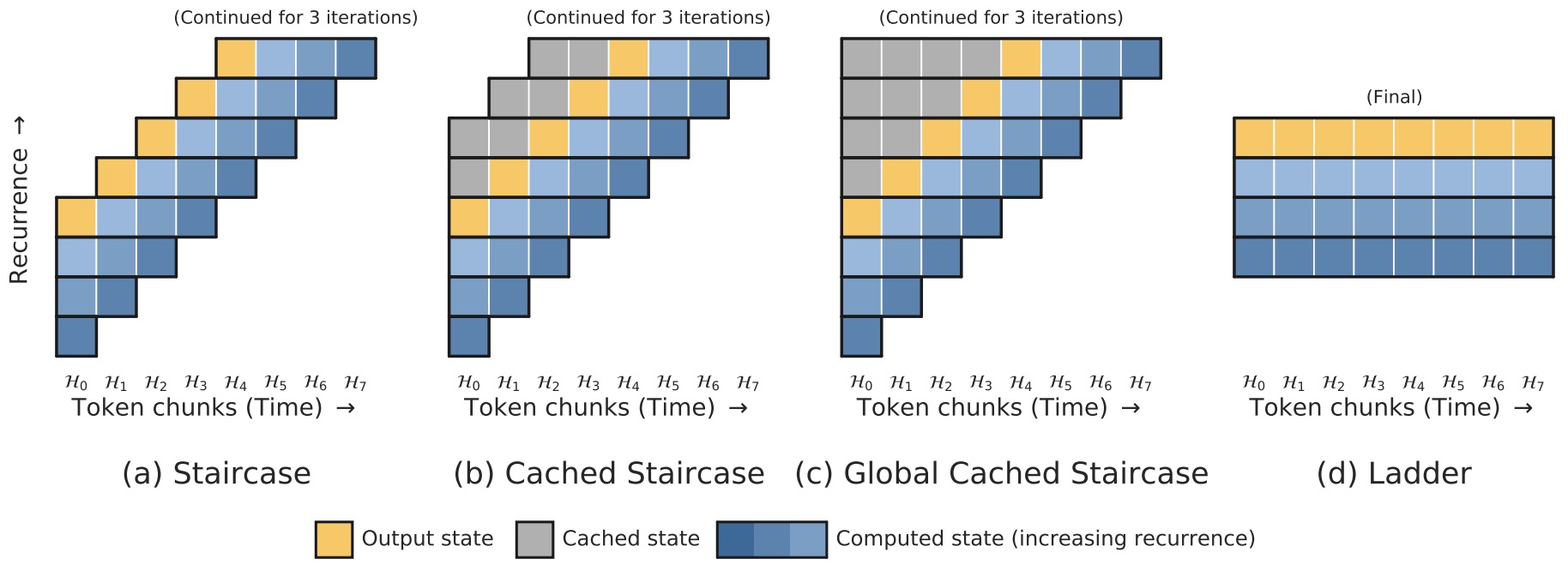
Ladder Variant
- The ladder variant is the most direct conceptual precursor to looped transformers. In ladder attention, the forward step is effectively removed, so the same transformer is applied repeatedly to an already available sequence. The sequence remains fixed, while only the hidden representation evolves:
-
This is precisely the computational pattern used in contemporary looped language models. Each recurrent step acts as another round of latent refinement, and the total amount of computation can be increased simply by executing more iterations.
-
The authors explicitly describe ladder attention as repeating the transformer with shared weights, making it an early and remarkably clear articulation of the looped-transformer paradigm.
Parameters and Compute
-
The key insight of staircase and ladder attention is that parameter count and computation should be treated independently. A model with a fixed number of parameters can be made substantially more powerful by performing more recurrent processing steps.
-
If a shared block contains \(N\) parameters and is executed \(L\) times, the effective computation scales approximately as:
\[C \propto N L\]- while the number of stored parameters remains \(N\).
-
This is exactly the principle that later became central to looped transformers, latent reasoning models, and adaptive test-time compute. The FAIR article Which one is more important: more parameters or more computation? articulates this argument directly and positions recurrent computation as an independent design dimension for deep learning systems.
Language Modeling Results
-
Ju et al. (2021) show that staircase attention yields lower perplexity than standard transformers of the same size and solves nonlinear state-tracking tasks that fixed-depth transformers struggle with. These results were an early empirical indication that repeated computation over the same parameters can unlock stronger reasoning and memory capabilities without requiring larger models.
-
In retrospect, these findings foreshadow the later success of recurrent-depth language models such as Huginn, Ouro, and Parcae, which scale this same principle to billions of parameters and trillions of tokens.
Relation to Looped Transformers
-
The connection between ladder attention and looped transformers is direct. Both architectures:
- Reuse the same parameters across multiple iterations
- Increase effective depth without increasing parameter count
- Enable test-time scaling by running more iterations
- Support latent reasoning rather than explicit chain-of-thought
- Expose computation as a runtime-adjustable resource
-
The main difference is historical emphasis. Staircase attention was introduced as a general recurrent attention mechanism for sequence modeling, while modern looped transformers focus specifically on reasoning, latent thought, and large-scale language modeling.
Historical Significance
-
The importance of staircase and ladder attention is that they established, as early as 2021, the core conceptual foundation that now drives much of the excitement around looped transformers. The architecture demonstrated that a transformer need not be a fixed stack of unique layers. Instead, it can be viewed as a reusable computational operator that is invoked repeatedly to refine an internal state.
-
This framing anticipated several major trends:
- Latent-space reasoning
- Adaptive inference depth
- Parameter-efficient scaling
- Separation of memory capacity from computational depth
-
As later work such as Scaling up Test-Time Compute with Latent Reasoning by Geiping et al. (2025) and Scaling Latent Reasoning via Looped Language Models by Zhu et al. (2025) demonstrates, this design principle has evolved into one of the most promising architectural directions for building models that can allocate additional internal computation to increasingly complex reasoning tasks.
Implementations
- Looped transformers are straightforward to implement because they preserve the internal structure of standard transformer blocks. The principal change is architectural rather than algorithmic: instead of instantiating a long stack of distinct modules, the model instantiates a smaller shared block and invokes it repeatedly inside a loop. This means that most existing transformer codebases can be adapted with relatively small modifications, making looped architectures practical both for research and for large-scale production systems.
Minimal Recurrence
- The simplest implementation wraps a standard transformer block in a Python loop:
class LoopedTransformer(nn.Module):
    def __init__(self, block, num_loops):
        super().__init__()
        self.block = block          # shared transformer block
        self.num_loops = num_loops

    def forward(self, x, attn_mask=None):
        h = x
        for _ in range(self.num_loops):
            h = self.block(h, attn_mask)
        return h
-
The critical detail is that
self.blockis a single module instance. Every recurrence step uses the same parameters, and gradients from all iterations accumulate into the shared weights during backpropagation. -
If the block contains \(k\) transformer layers and is executed \(L\) times, the effective depth becomes:
- This is the core implementation pattern underlying most modern looped architectures.
Prelude and Coda
- In large language models, the recurrent block is often surrounded by non-shared layers that specialize the beginning and end of computation:
def forward(tokens):
    h = embed(tokens)
    h = prelude(h)
    for _ in range(num_loops):
        h = recurrent_core(h)
    h = coda(h)
    return lm_head(h)
- This pattern appears explicitly in Scaling Latent Reasoning via Looped Language Models by Zhu et al. (2025), where the model consists of an embedding layer, optional prelude layers, a recurrent core, an exit mechanism, and a language modeling head.
Relaxed Sharing
-
Strict parameter tying maximizes compression but may reduce representational flexibility. A common compromise adds lightweight, loop-specific adapters to the shared block:
\[\theta_t =\theta + \Delta \theta_t\]- where \(\Delta \theta_t\) is typically a low-rank LoRA update.
-
In code, each loop can activate its own adapter while keeping the main weights shared. Relaxed Recursive Transformers: Effective Parameter Sharing with Layer-wise LoRA by Bae et al. (2025) shows that this approach recovers much of the performance of untied models while preserving most of the parameter savings.
Adaptive Exits
- To avoid using unnecessary computation, many implementations attach a small exit head that predicts whether further recurrence is needed:
for step in range(max_loops):
    h = recurrent_core(h)
    exit_prob = exit_head(h)
    if exit_prob.mean() > threshold:
        break
-
The stopping rule can be applied at the sequence level, token level, or batch element level.
-
Scaling Latent Reasoning via Looped Language Models by Zhu et al. (2025) uses an entropy-regularized exit gate to allocate computation dynamically across examples.
Token Routing
-
A more granular design routes individual tokens rather than entire sequences. At each loop, a lightweight router determines which tokens continue participating in computation and which are skipped.
-
Mixture-of-Recursions: Learning Dynamic Recursive Depths for Adaptive Token-Level Computation by Bae et al. (2025) implements this strategy so that only active tokens incur attention and key-value cache costs, significantly improving throughput.
-
Conceptually, each token receives its own depth assignment:
\[L_i = g(x_i)\]- where \(L_i\) is the number of recursions allocated to token \(i\).
Key-Value Caching
-
During autoregressive generation, each loop can either compute fresh key-value projections or reuse previously computed values.
-
The most direct implementation recomputes keys and values at every recurrence, preserving full flexibility but increasing cost. Some architectures share key-value tensors across loops to reduce memory and bandwidth requirements. Mixture-of-Recursions: Learning Dynamic Recursive Depths for Adaptive Token-Level Computation by Bae et al. (2025) introduces a KV-sharing variant that reuses the first recursion’s cache.
-
The following figure (source) shows the architectural components of Mixture-of-Recursions (MoR), including expert-choice routing, token-choice routing, and the caching mechanism for recursive token computation (i.e., recursive key-value caching). In expert-choice routing, a router selects the top-\(k\) tokens at each recursion step to continue computing, progressively narrowing the active token set as depth increases. In token-choice routing, each token receives a fixed recursion step assignment at the outset through a single routing decision, which defines its full compute path through the model. In the KV caching panels, each square in the matrix indicates whether a token row attends to another token’s cached key column: in recursion-wise KV caching, shown in blue, only the keys of currently selected non-dropped tokens are cached at each recursion step and attention is restricted to those entries; in recursive KV sharing, shown in purple, all keys of previous tokens are cached at the first recursion step and then shared across subsequent recursion steps for attention.
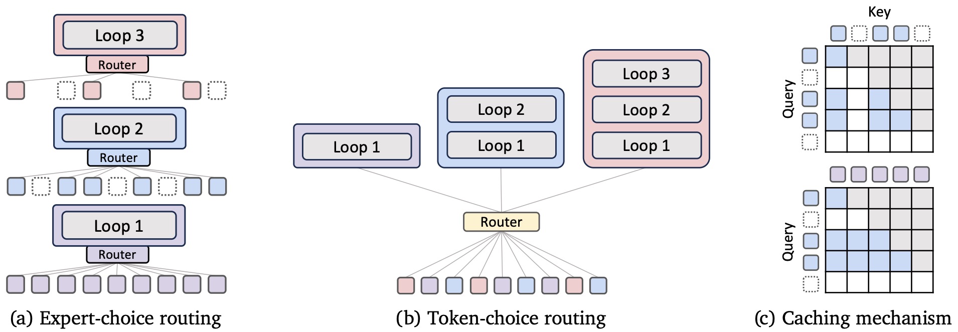
Memory and Checkpointing
- Although parameter memory is reduced, activation memory grows with the number of unrolled iterations. Training deep recurrence therefore benefits from activation checkpointing:
for _ in range(num_loops):
    h = checkpoint(recurrent_core, h)
- Checkpointing recomputes activations during the backward pass and is often essential when loop counts become large.
Conversion from Pretrained Models
-
Existing transformers can be converted into recursive models by grouping layers into a shared block and reusing that block repeatedly. A simplified procedure is:
- Select a subset of layers.
- Tie their weights.
- Initialize a recurrent core.
- Uptrain on additional data.
- Optionally add LoRA adapters.
-
This approach allows strong recursive models to be built from existing checkpoints rather than trained from scratch. Relaxed Recursive Transformers: Effective Parameter Sharing with Layer-wise LoRA by Bae et al. (2025) demonstrates recursive conversions of Gemma and related models.
Open Implementations
-
Several open-source implementations make looped architectures accessible:
- Ouro Project Page provides pretrained looped language models and evaluation results.
- recurrent-pretraining contains the Huginn recurrent-depth training code released alongside Geiping et al. (2025).
- OpenMythos is a community implementation inspired by speculative reconstructions of Claude Mythos and combines recurrent depth with Mixture-of-Experts and configurable attention.
-
These projects demonstrate that looped transformers can be integrated into conventional PyTorch and distributed-training pipelines with relatively modest engineering effort.
Engineering View
-
From an engineering perspective, looped transformers are appealing because they reuse well-understood components. The innovation lies in how those components are scheduled. A standard transformer can be reinterpreted as a reusable computational operator, and recurrence turns that operator into an iterative refinement engine.
-
This makes looped architectures unusually practical: they inherit the mature tooling, kernels, and optimization strategies developed for conventional transformers, while adding the ability to scale computation dynamically, compress parameters, and perform latent reasoning through repeated application of a shared block.
Open Questions
- Looped transformers have rapidly evolved from a theoretical curiosity into a serious architectural alternative for large-scale language models, but many of their most important properties remain only partially understood. The current literature establishes that recurrence can improve reasoning, parameter efficiency, and adaptive inference, yet several foundational questions remain open around optimization, expressivity, interpretability, convergence, and deployment.
Optimal Sharing
- One of the central design questions is how much parameter sharing should be enforced. At one extreme, strict tying uses exactly the same weights at every iteration:
- At the other extreme, every layer has independent parameters, as in a conventional transformer. Between these endpoints lie partially shared models, such as relaxed recursive transformers with loop-specific LoRA updates:
- Relaxed Recursive Transformers: Effective Parameter Sharing with Layer-wise LoRA by Bae et al. (2025) demonstrates that small low-rank adaptations can recover much of the performance lost under strict tying, which suggests that the best architectures may sit between fully tied loops and fully independent layers. The broader unresolved question is what degree of sharing best balances compression, expressivity, generalization, and optimization.
Learned Halting
-
Although adaptive computation is one of the most attractive features of looped transformers, robust halting remains an open challenge. Exit mechanisms must detect when the hidden state contains sufficient information while avoiding both premature stopping and unnecessary extra computation.
-
A typical stopping rule takes the form:
\[\text{stop if } p_{\mathrm{exit}}(h_t) > \tau\]- where \(p_{\mathrm{exit}}\) is predicted by a lightweight classifier and \(\tau\) is a threshold.
-
Scaling Latent Reasoning via Looped Language Models by Zhu et al. (2025) presents Ouro models with iterative latent computation and learned depth allocation, while Mixture-of-Recursions: Learning Dynamic Recursive Depths for Adaptive Token-Level Computation by Bae et al. (2025) combines recursive parameter sharing with routers that assign different recursion depths to different tokens. The open problem is not only whether a model can halt, but whether the halting signal is reliable, interpretable, calibrated, and robust under distribution shift.
Mechanistic Understanding
-
Why does recurrence improve reasoning so dramatically? Existing evidence suggests that looping encourages iterative retrieval, search, and composition, but the precise circuits responsible for these behaviors are not yet fully understood.
-
Loop, Think, & Generalize: Implicit Reasoning in Recurrent-Depth Transformers by Kohli et al. (2026) studies recurrent-depth transformers for implicit multi-hop reasoning and reports that recurrence helps systematic generalization and depth extrapolation, while also identifying overthinking as a limitation.
-
Important unanswered questions include:
- Loop phases: Do early loops perform pattern matching while later loops perform abstraction, verification, or refinement?
- State convergence: Can hidden-state trajectories reveal when a model has reached a stable answer?
- Task dependence: Do math, code, graph search, retrieval, and planning use recurrence in different ways?
- Circuit reuse: Does the same recurrent block implement genuinely different computations at different loop depths, or does it mostly repeat one refinement operation?
- Interpretability: Can loop trajectories be probed in a way that is as useful as probing attention heads or MLP features in ordinary transformers?
Convergence Criteria
-
Most current systems specify a fixed maximum loop count or rely on learned exit probabilities. A more principled approach would detect whether the recurrent state has converged.
-
One simple criterion is:
\[\lVert h_{t+1} - h_t \rVert < \varepsilon\]- where \(\varepsilon\) is a convergence threshold.
-
However, hidden-state stability does not necessarily imply correctness. A model can converge to the wrong answer, oscillate among plausible states, or appear stable while still lacking a needed compositional step. Designing convergence diagnostics that correlate with task success remains an open challenge with direct implications for adaptive inference.
Overthinking
-
Additional recurrence often improves performance up to a point, after which accuracy may decline as the model overwrites useful representations:
\[\mathrm{Acc}(L+1) < \mathrm{Acc}(L)\]- for sufficiently large \(L\).
-
This overthinking phenomenon, highlighted in Loop, Think, & Generalize: Implicit Reasoning in Recurrent-Depth Transformers by Kohli et al. (2026), suggests that recurrent operators may not always move toward a stable useful fixed point. Understanding why overthinking occurs, and how to prevent it with halting, loop regularization, convergence tests, or depth-conditioned adaptation, is essential for reliable test-time scaling.
Multimodal Recurrence
-
Most current looped language-model work focuses on text, but recurrence is equally applicable to multimodal architectures. Vision transformers, audio models, robotics policies, and multimodal agents could all benefit from adaptive iterative processing, especially when perception or planning naturally requires repeated refinement.
-
The success of iterative recycling in systems such as AlphaFold has strengthened interest in applying recurrence beyond language. The unresolved question is whether looped multimodal systems can reliably improve visual search, spatial reasoning, video understanding, embodied planning, and cross-modal grounding without creating unstable recurrent dynamics or excessive latency.
Hardware Scheduling
-
Looped transformers change the computational profile of inference. They reduce parameter memory but increase sequential depth, and adaptive routing introduces irregular workloads where different tokens and examples require different numbers of iterations.
-
This raises systems-level questions about:
- Batching: How should examples with different loop counts be batched efficiently?
- KV cache reuse: Which keys and values can be reused across recursions without hurting quality?
- Dynamic exits: How should hardware schedule tokens that halt at different depths?
- Memory bandwidth: Can recurrence reduce memory pressure enough to offset additional sequential compute?
- Throughput: Can looped models improve serving economics by fitting strong reasoning into fewer stored parameters?
-
Mixture-of-Recursions: Learning Dynamic Recursive Depths for Adaptive Token-Level Computation by Bae et al. (2025) addresses part of this by allowing token-level adaptive recursion while improving throughput, and Relaxed Recursive Transformers: Effective Parameter Sharing with Layer-wise LoRA by Bae et al. (2025) discusses continuous depth-wise batching as an inference paradigm enabled by recursive transformers.
Scaling Limits
-
Current evidence shows that recurrence can substitute for large amounts of explicit depth, but it remains unclear how far this substitution extends. Open questions include whether looped architectures can dominate standard transformers at frontier scale, whether recurrence remains advantageous as models approach hundreds of billions or trillions of parameters, and how much training data is required to fully exploit deeper latent computation.
-
Parcae: Scaling Laws for Stable Looped Language Models by Prairie et al. (2026) provides early scaling laws for stable looped models, including the finding that compute-optimal training should scale recurrence and data together under a fixed FLOP budget.
-
The key unresolved issue is whether loop depth becomes a durable third scaling axis alongside parameters and data:
- If this holds at large scale, looped transformers could make inference-time depth a first-class architectural resource.
Architectural Outlook
-
The open question is no longer merely whether looped transformers can work in small controlled settings. The sharper question is whether recurrence can become a durable component of frontier-scale model design.
-
Several signs point in that direction:
- Parameter efficiency: Looped transformers decouple stored weights from effective depth.
- Inference-time scaling: More loops can increase compute on hard examples without changing model size.
- Latent reasoning: Recurrent-depth models can reason internally without generating long chains of thought.
- Adaptive computation: Routers, halting heads, and continuous depth-wise batching make it possible to spend different amounts of compute on different tokens, examples, or tasks.
- Serving economics: If recurrence reduces memory footprint while preserving or improving capability, it directly addresses one of the central bottlenecks in frontier-model deployment.
- Hybridization: Recurrence can be combined with MoE, MLA/GQA, LoRA-style loop adaptation, retrieval, tool use, or RLM-style outer recursion.
-
Regardless of any specific commercial implementation, the research trajectory is increasingly clear. Looped transformers provide a principled way to separate memory from computation, allocate depth dynamically, and reason internally in latent space. Whether as a replacement for fixed-depth transformers or as a component within larger hybrid systems, recurrence appears poised to play a central role in the next phase of language model architecture.
Claude Mythos Speculation
-
Public discussion around Claude Mythos has become one of the clearest examples of why looped transformers matter architecturally. The claim is not verified: Anthropic has not released enough technical detail to confirm Claude Mythos’s architecture. The section is best read as an architectural outlook, not as a confirmed model report.
-
The useful idea is that future frontier systems may increasingly decouple stored capacity from runtime reasoning depth. Looped transformers make that decoupling explicit: a model can be made stronger not only by adding more parameters, but also by giving the same parameters more opportunities to refine hidden states. Whether or not Claude Mythos uses this design, the speculation captures a broader trend toward combining parameter-efficient recurrence, adaptive latent compute, MoE breadth, and systems-level scaffolding.
-
The public hypothesis is that Claude Mythos may be a Recurrent-Depth Transformer, or looped transformer, where a fixed set of layers is reused multiple times inside a single forward pass. In this view, the model’s reasoning depth is not determined only by the number of unique layers it stores; it is also determined by how many recurrent iterations it runs at inference time.
OpenMythos
-
OpenMythos is a community reconstruction that tries to make the Claude Mythos hypothesis concrete. It explicitly describes itself as independent, speculative, and not affiliated with Anthropic. The repository proposes a three-stage architecture: Prelude, looped Recurrent Block, and Coda, with attention switchable between GQA and MLA and feed-forward layers implemented as sparse MoE experts.
-
The proposed structure is:
\[\text{Input} \rightarrow P \rightarrow R^T \rightarrow C \rightarrow \text{Output}\]- where \(P\) is the prelude, \(R\) is the recurrent block, \(T\) is the number of recurrent loop iterations, and \(C\) is the coda.
-
The recurrent update is described as:
\[h_{t+1} = A h_t + B e + \mathrm{Transformer}(h_t, e)\]- where \(h_t\) is the hidden state after loop \(t\), \(e\) is the encoded input from the prelude, and \(A, B\) are learned injection parameters. The repeated injection of \(e\) is meant to preserve the input signal across loop depth and reduce hidden-state drift.
Why people connected Mythos to looping
-
The strongest public argument is based on the distinction between memorized knowledge and reasoning depth. A looped model may not memorize more facts at a fixed parameter count, but it can get better at manipulating what it already knows by spending more recurrent compute.
-
The “Looped Transformers Controversy” thread makes this argument explicitly: the author warns that the claim is speculative, then points to benchmark patterns where Claude Mythos appears to improve modestly on knowledge-heavy benchmarks but much more sharply on reasoning-heavy benchmarks such as graph search. The proposed interpretation is that Mythos may represent a modest parameter scale-up but a more aggressive depth scale-up.
-
The following figure (source) shows the benchmark screenshot used in the public speculation: Claude Mythos Preview appears much stronger on reasoning-heavy graph-walk and coding-style benchmarks than on more knowledge-heavy rows, motivating the hypothesis that recurrence may increase reasoning depth more than memorized knowledge.
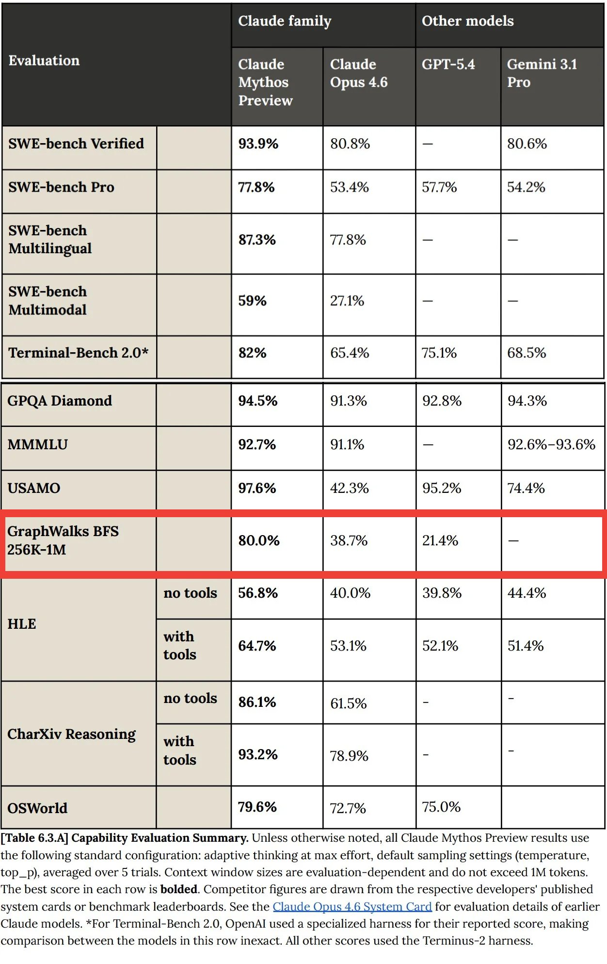
-
The same thread connects this to looped-transformer experiments where looped and non-looped models can have similar memorization capacity at the same parameter count, while the looped variants perform much better on reasoning-heavy tasks.
-
The following figure (source) shows the knowledge-capacity versus reasoning-performance comparison used in the speculation. (Left) looped and standard transformer baselines with the same parameter count are trained on the Capo task to compare whether looping increases knowledge capacity; at fixed parameter count, the looped model and its non-looped baseline have almost the same knowledge capacity, measured in bits of knowledge on Capo. (Right) accuracy of looped and non-looped models on the Mano task; looped models outperform the iso-parameter \({2,3,6} \otimes 1\) baselines and achieve better or comparable performance relative to the iso-FLOP \(12 \otimes 1\) baseline.
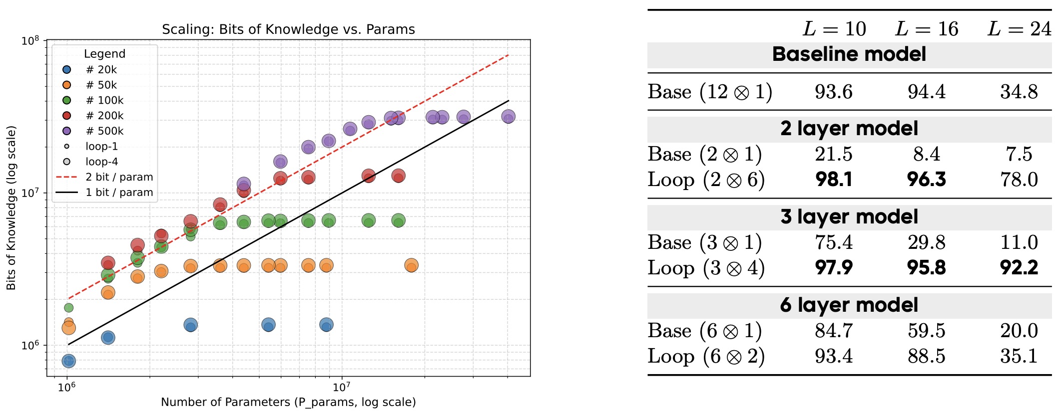
Implicit reasoning hypothesis
-
Another part of the Claude Mythos speculation comes from work on implicit multi-hop reasoning. The hypothesis is that looped transformers can combine parametric knowledge in ways that ordinary fixed-depth transformers struggle to do.
-
Loop, Think, & Generalize: Implicit Reasoning in Recurrent-Depth Transformers by Kohli et al. (2026) studies whether recurrent-depth transformers can compositionally use parametric knowledge for implicit multi-hop reasoning, focusing on systematic generalization and depth extrapolation. The paper argues that vanilla transformers often store knowledge but fail to flexibly compose it, while recurrent-depth transformers can reuse the same layers iteratively to access and combine parametric knowledge inside a single forward process.
-
The following figure (source) shows the recurrent depth model architecture. The transformer block is repeated \(R\) times. The embedding layer and language model head have tied weights. In the paper’s experiments, the authors use a simple looped transformer similar to Saunshi et al. (2025), without input injection, gated halting, or middle looping.**

- The architectural point is simple but important: a GPT-style block with \(L\) layers is reused for \(R\) recurrent iterations, giving an effective rolled-out depth of:
-
At each recurrent iteration, the same stack of layers is applied to the current hidden states:
\[h^{(r+1)} = f_\theta(h^{(r)}; m), \quad r = 0,\ldots,R-1\]- where \(f_\theta\) is the shared transformer block and \(m\) denotes the causal attention and padding masks. This lets the model increase inference-time computation by increasing \(R\) without changing the architecture or retraining parameters.
-
The following figure (source) shows an illustration of systematic and extrapolation generalization tasks with a sample dataset. The task is built from a directed knowledge graph where atomic 1-hop facts have the form \((h,r,t)\), and a \(k\)-hop inferred fact is a chain of atomic facts connecting a head entity to a final tail through intermediate entities. Systematic generalization evaluates inferred facts composed from atomic facts that were never used in training compositions, while depth extrapolation evaluates inferred facts with more hops than those included in training.
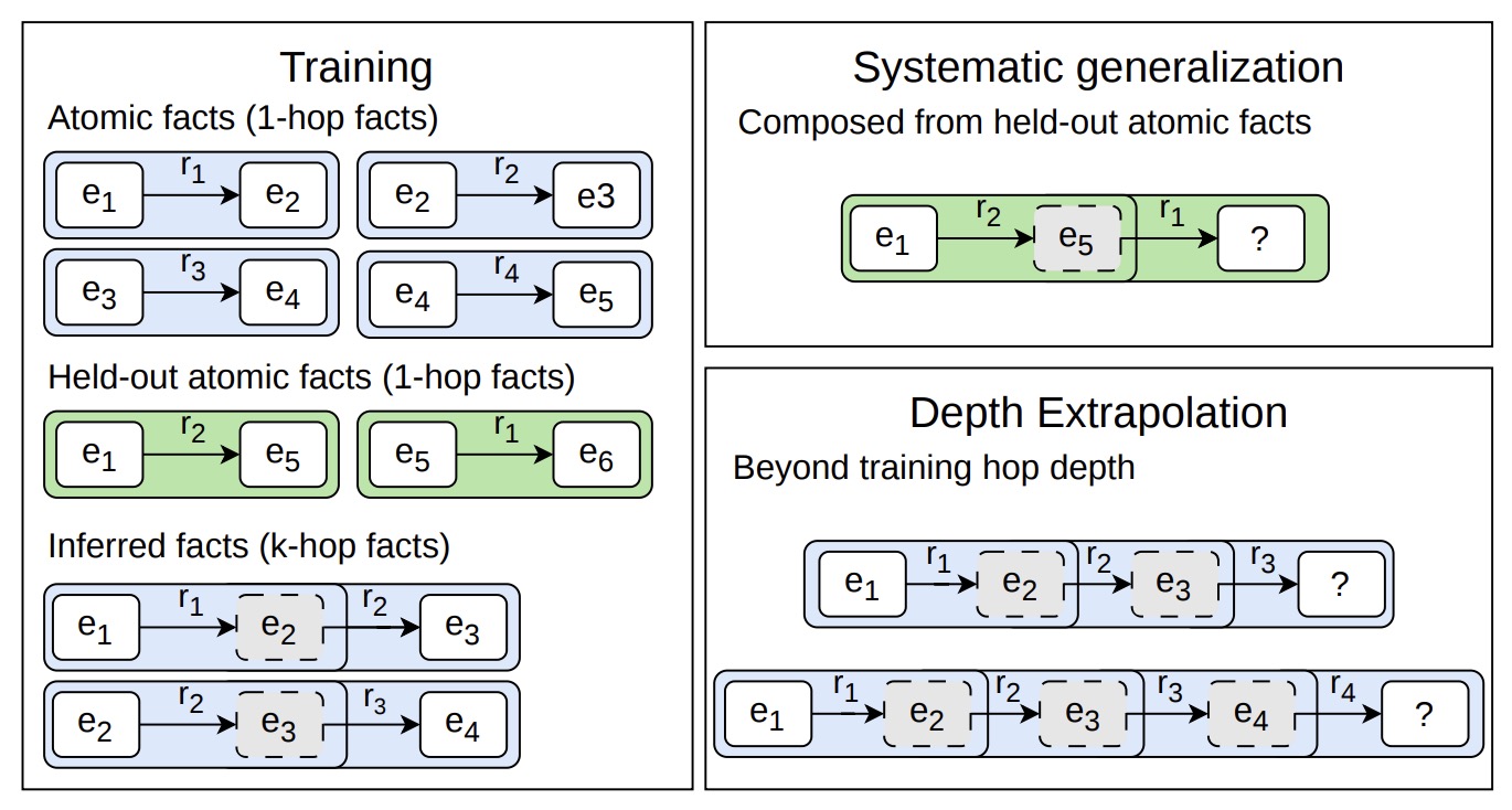
- This is why the Mythos speculation focuses on graph-search and multi-step reasoning benchmarks. Those tasks stress composition more than stored factual recall. If a model can run more latent loops at inference time, it may be able to perform more steps of implicit reasoning without emitting a long chain of thought.
Suspected architecture
-
The OpenMythos reconstruction combines several ideas from recent looped-transformer research into one speculative frontier-style design:
- Prelude, recurrent block, coda: The prelude encodes the input once, the recurrent block performs repeated latent refinement, and the coda maps the final recurrent state to output tokens.
- Input reinjection: The encoded input \(e\) is reintroduced at every recurrent step so the hidden state does not drift too far from the original prompt.
- MoE breadth plus looped depth: Sparse MoE feed-forward layers provide broad domain capacity, while recurrence provides deeper reasoning over the same activated representation.
- MLA or GQA attention: Multi-Latent Attention compresses KV state, while Grouped Query Attention reduces KV heads; both are plausible choices for improving memory efficiency in recurrent-depth inference.
- Stability constraints: A Parcae-like dynamical-systems view suggests constraining recurrence so the spectral radius remains below one: \(\rho(A) < 1\).
- Loop-index embeddings: A loop-position signal could let the same weights behave differently at different recurrence depths, making each loop a distinct computational phase rather than a literal repetition.
- Adaptive halting: A learned exit rule or convergence criterion could prevent the model from running the maximum number of loops on every token or request.
- Continuous depth-wise batching: Different tokens, sequences, or requests could exit at different depths while sharing the same recurrent block, improving serving efficiency.
-
The following figure (source) shows the OpenMythos summary table of the hypothesized architecture: Recurrent-Depth Transformer structure, suspected MoE FFN, implicit multi-hop reasoning through latent updates, stability via spectral-radius control, possible loop-index embeddings, adaptive halting, MLA/GQA attention, and continuous depth-wise batching.
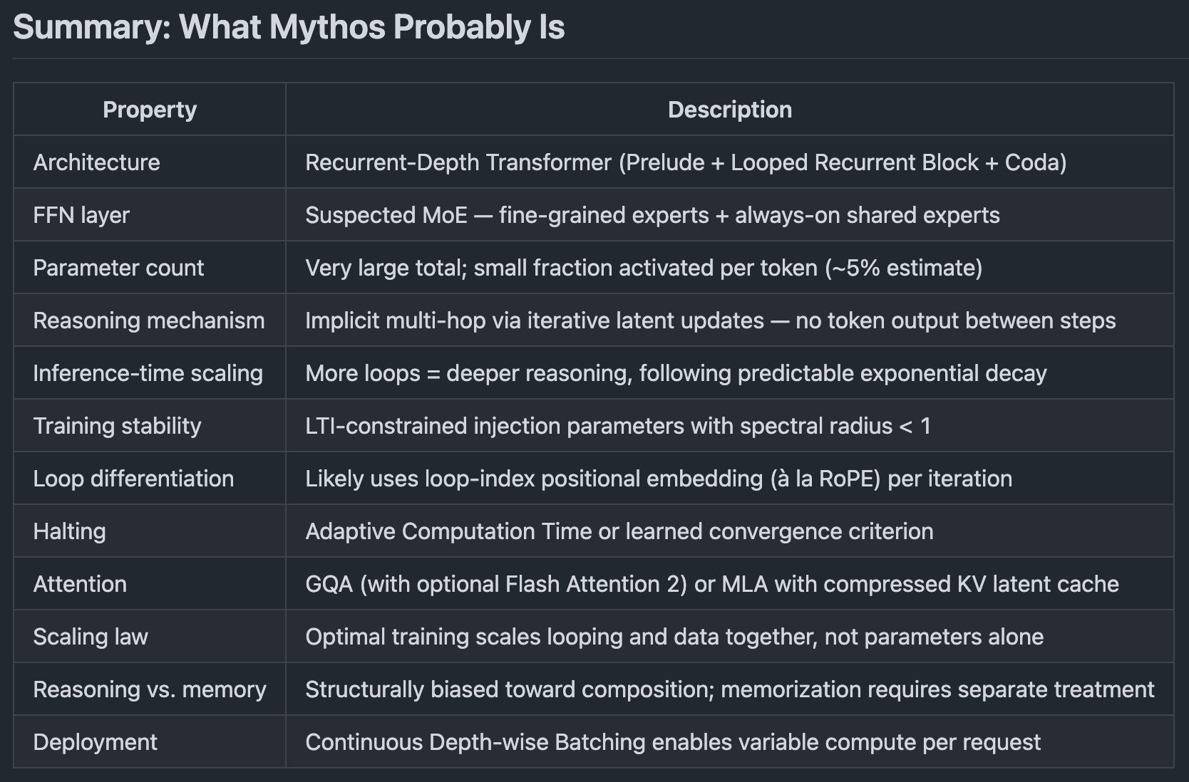
- A compact version of the hypothesis is:
What the speculation gets right
-
Even if Claude Mythos itself turns out not to be a looped transformer, the architectural logic is important. Specifics below:
- It separates memory from reasoning: Parameters store capabilities and knowledge; recurrent loops provide extra computation for manipulating them.
- It explains reasoning-heavy gains: Looping should help most when the task requires multi-step composition, search, planning, or graph traversal.
- It fits serving constraints: If a model can get stronger reasoning at a lower parameter footprint, it may reduce memory pressure and improve deployment economics.
- It aligns with latent reasoning research: Looped and recurrent-depth models provide a way to increase computational graph depth without generating more tokens.
- It motivates hybrid architectures: A frontier model could combine recurrence, MoE, KV compression, adaptive halting, and tool or RLM-style outer scaffolds.
What remains unknown
-
The speculative Claude Mythos story should not be treated as evidence of Anthropic’s actual architecture. Several questions remain unanswered:
- Architecture: It is unknown whether Mythos uses strict looping, partial layer sharing, recurrent-depth blocks, adaptive recurrence, or something else entirely.
- Halting: It is unknown whether compute depth is fixed, token-adaptive, sequence-adaptive, or controlled by a learned exit head.
- MoE: It is unknown whether MoE is involved, how many experts exist, or what fraction of parameters are activated per token.
- Stability: It is unknown whether any Parcae-like spectral constraint, input reinjection, or loop-index embedding is used.
- Benchmark interpretation: Strong results on reasoning-heavy benchmarks are suggestive but not diagnostic; many architectural and training choices could produce similar patterns.
- Parameter count: Public benchmark behavior cannot reliably identify whether capability comes from more parameters, more data, better post-training, better tools, recurrence, or a combination.
Recursive Latent Reasoning
Overview
-
Recursive latent reasoning is a way to spend more computation inside the model’s hidden state before producing an answer. Instead of writing a long chain-of-thought, the model repeatedly updates latent vectors that represent its current reasoning state.
-
A standard predictor computes one pass:
- A recursive latent reasoner computes multiple internal refinements:
-
The important shift is:
- The model does not externalize reasoning as text: Reasoning happens through hidden vectors, not natural-language steps.
- The same parameters are reused: Recursion increases effective depth without proportionally increasing parameter count.
- The output can improve over iterations: Each recurrent update gives the model another chance to repair, refine, or complete the answer.
- The system can be trained without chain-of-thought traces: Supervision can be applied only to final answers or repeated answer refinements.
- The method is especially natural for structured puzzles: Sudoku, mazes, and ARC-style grid tasks require iterative constraint propagation, search, correction, and refinement.
-
Hierarchical Reasoning Model by Wang et al. (2025) introduces a recurrent architecture with high-level and low-level modules operating at different timescales, while Less is More: Recursive Reasoning with Tiny Networks by Jolicoeur-Martineau (2025) simplifies the idea into a single tiny recursive network that repeatedly refines its latent state and answer.
Why this differs from chain-of-thought
- Chain-of-thought reasoning spends compute by generating more tokens:
- Recursive latent reasoning spends compute by updating hidden states:
-
The distinction matters because token-level reasoning is constrained by language. Every intermediate step must be serializable as text, and an early wrong token can derail the rest of the solution. Latent reasoning can represent partial states, alternatives, constraints, and corrections without committing to a word sequence.
-
The practical tradeoff is:
- Chain-of-thought is interpretable: The intermediate reasoning is visible, easy to inspect, and easy to prompt.
- Latent recursion is compact: The intermediate reasoning is hidden, dense, and can be much cheaper than producing long traces.
- Chain-of-thought can be brittle: A wrong verbal step may propagate through the solution.
- Latent recursion can self-correct internally: The model can repeatedly refine an answer representation before emitting the final output.
- Chain-of-thought usually needs language data or RL traces: Recursive latent models can be trained directly from input-output examples when the task has dense supervised targets.
-
Training Large Language Models to Reason in a Continuous Latent Space by Hao et al. (2024) motivates this broader direction by arguing that language is not always the optimal space for reasoning, while HRM and TRM instantiate the idea in compact recurrent architectures for puzzle-solving rather than language modeling.
HRM at a glance
-
HRM uses two recurrent modules:
- High-level module: Maintains a slower, more abstract state that guides reasoning across phases.
- Low-level module: Performs faster, detailed computation conditioned on the high-level state.
- Input network: Converts the task input into a working representation.
- Output network: Converts the final latent state into a task prediction.
- Multi-timescale recurrence: The low-level module runs several steps while the high-level state stays fixed; then the high-level module updates and starts a new phase.
- Single forward-pass solving: The model performs iterative latent computation internally and emits the final answer without generating explicit reasoning text.
-
A simplified view is:
\[\tilde{x} = f_I(x)\] \[z_L^{i} = f_L(\tilde{x}, z_L^{i-1}, z_H^{c})\] \[z_H^{c+1} = f_H(\tilde{x}, z_H^{c}, z_L^{cT})\] \[\hat{y} = f_O(z_H^N, z_L^{NT})\]- where \(z_H\) is the high-level state, \(z_L\) is the low-level state, \(T\) is the number of low-level steps per high-level cycle, and \(N\) is the number of high-level cycles.
-
Hierarchical Reasoning Model by Wang et al. (2025) reports that HRM uses about 27M parameters, trains from roughly 1000 examples, and targets puzzle-style reasoning tasks such as Sudoku-Extreme, Maze-Hard, and ARC-AGI without pretraining or chain-of-thought supervision.
-
The following figure (source) shows HRM’s two-timescale recurrent design, hierarchical inspiration, and benchmark comparison. On the left, HRM is motivated by hierarchical processing and temporal separation in the brain, with two recurrent networks operating at different timescales: a high-level module for slower abstract planning and a low-level module for faster detailed computation. On the right, a ~27M-parameter HRM trained on about 1000 examples is compared against chain-of-thought and direct-prediction baselines, outperforming them on ARC-AGI, Sudoku-Extreme, and Maze-Hard.
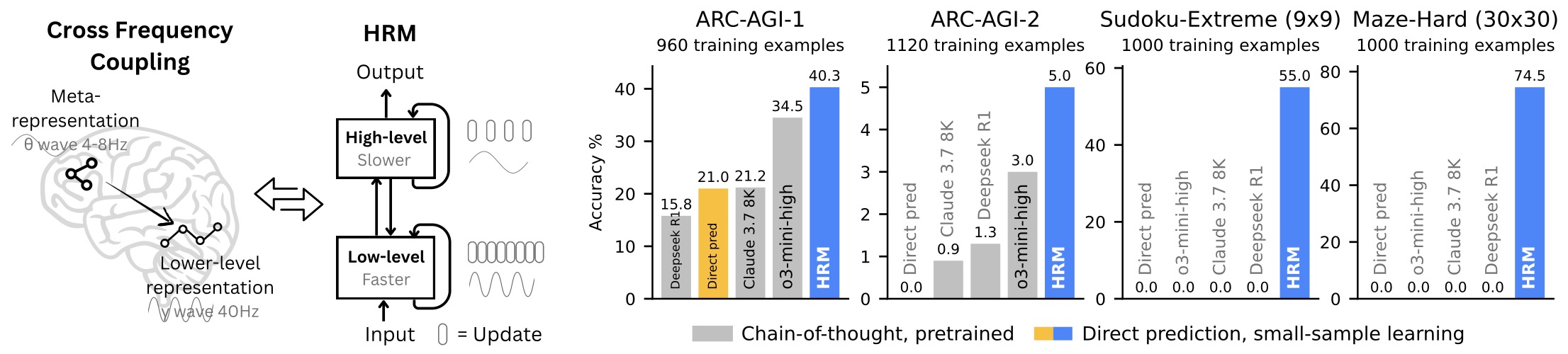
TRM at a glance
-
TRM removes HRM’s hierarchy. Instead of using separate high-level and low-level networks, it uses one tiny recursive network to update a latent reasoning state and refine the answer.
-
A simplified TRM loop is:
\[z^{i+1} = f_\theta(x, y^i, z^i)\] \[y^{i+1} = f_\theta(y^i, z^{i+1})\]- where \(x\) is the embedded input, \(y^i\) is the current answer representation, and \(z^i\) is the latent reasoning state.
-
The core design is:
- One recursive network: TRM replaces HRM’s two-module hierarchy with one small network.
- Two latent features: TRM keeps a latent reasoning feature \(z\) and an answer feature \(y\).
- Nested recursion: The model performs several latent updates before each supervised answer refinement.
- Deep supervision: The model is supervised over repeated refinement steps, so later predictions should improve.
- Optional early stopping: A Q-head can predict whether the current answer is already correct.
- Parameter efficiency: TRM reports strong results with only a few million parameters.
-
Less is More: Recursive Reasoning with Tiny Networks by Jolicoeur-Martineau (2025) argues that the hierarchy and fixed-point justification in HRM are not necessary for strong recursive reasoning, and reports that TRM improves over HRM on Sudoku-Extreme, Maze-Hard, ARC-AGI-1, and ARC-AGI-2 with fewer parameters.
-
The following figure (source) shows TRM recursively refining its predicted answer through repeated latent updates using an embedded input, an answer state, and a latent reasoning state over repeated supervision steps. This illustrates why evaluation should track prediction quality across refinement steps rather than only after one pass.
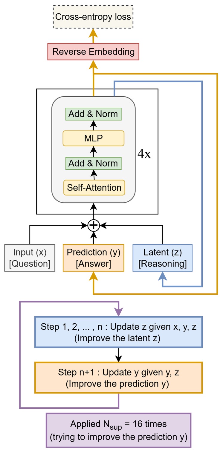
The HRM-to-TRM simplification
-
TRM can be read as a critique and simplification of HRM. HRM proposes a biologically inspired hierarchy; TRM asks which parts are actually necessary for generalization.
-
The simplification is:
- From two networks to one network: HRM uses separate high-level and low-level modules; TRM uses one recursive network.
- From hierarchy to recurrence: HRM interprets reasoning through slow and fast timescales; TRM treats recursive answer improvement as the central mechanism.
- From fixed-point assumptions to direct recursion: HRM motivates training through convergence-style reasoning; TRM trains repeated refinements directly.
- From complex halting to simpler stopping: TRM uses an output head and Q-head without requiring HRM’s extra forward-pass style halting machinery.
- From architectural explanation to ablation-driven explanation: TRM emphasizes that simple repeated refinement can be enough for strong performance on these tasks.
-
TRM reports that, on Sudoku-Extreme, a 5M-parameter TRM reaches 87.4% test accuracy in its reported ablation table, compared with HRM’s 55.0% at 27M parameters; with attention, TRM reports 85.3% on Maze-Hard, 44.6% on ARC-AGI-1, and 7.8% on ARC-AGI-2, compared with HRM’s 74.5%, 40.3%, and 5.0% in the same comparison.
Connection to looped transformers
-
Looped transformers apply the same principle at transformer scale: reuse a block of layers multiple times to increase effective depth. HRM and TRM apply the principle to compact puzzle-solving networks.
-
The shared pattern is:
-
The differences are:
- Looped transformers operate over token sequences: They reuse transformer blocks over hidden token representations.
- HRM operates over hierarchical latent states: It separates slow abstract planning from fast local computation.
- TRM operates over answer and latent state features: It repeatedly improves an answer representation with one tiny network.
- RLMs operate outside the model: They recurse through model calls and environment state rather than through hidden activations.
-
Scaling up Test-Time Compute with Latent Reasoning: A Recurrent Depth Approach by Geiping et al. (2025) scales test-time compute by iterating a recurrent language-model block, and Reasoning with Latent Thoughts: On the Power of Looped Transformers by Saunshi et al. (2025) analyzes how looped transformers can emulate multi-step reasoning through repeated latent computation.
Connection to RLMs
-
RLMs and recursive latent reasoning solve different levels of the problem.
-
RLMs recurse over external context:
- HRM and TRM recurse over internal state:
-
The relationship is:
- RLMs are good at context control: They decide what evidence to inspect, how to split work, and how to aggregate child outputs.
- HRM and TRM are good at compact iterative reasoning: They refine solutions internally without emitting reasoning text.
- RLMs are inspectable: Their intermediate state is a trajectory.
- HRM and TRM are opaque: Their intermediate state is latent.
- RLMs can wrap latent recursive models: A future RLM could use HRM-like or TRM-like models as child solvers for structured subproblems.
- Latent recursive models can strengthen RLM calls: A child model with better internal refinement may need fewer external calls.
-
The conceptual bridge is that both approaches treat reasoning as repeated computation, not merely as one feedforward pass or one long generated explanation.
Architecture
Design objective
-
Recursive latent reasoning models are built around one core objective: increase effective reasoning depth without producing long text traces and without scaling parameter count.
-
A conventional feedforward model has a fixed amount of computation:
- A recursive latent model reuses a smaller computation block many times:
-
The design priorities are:
- Effective depth: The model should perform many internal refinement steps even if it has few layers.
- Parameter reuse: The same network or modules are reused across recursive steps.
- Latent state: Intermediate reasoning is stored in vectors rather than generated as natural language.
- Final-answer supervision: The model can be trained from input-output pairs without annotated reasoning chains.
- Iterative correction: Later steps can revise earlier answer states rather than committing after one pass.
-
Hierarchical Reasoning Model by Wang et al. (2025) uses two coupled recurrent modules for multi-timescale latent reasoning, while Less is More: Recursive Reasoning with Tiny Networks by Jolicoeur-Martineau (2025) simplifies the design to one tiny recursive network with repeated answer refinement.
HRM components
-
HRM contains four learnable parts:
- Input network \(f_I\): Projects the raw task input \(x\) into a working representation \(\tilde{x}\).
- Low-level recurrent module \(f_L\): Performs fast, detailed computation over the working representation, its own state, and the current high-level state.
- High-level recurrent module \(f_H\): Performs slower abstract updates after the low-level module has run for multiple steps.
- Output network \(f_O\): Converts the final latent states into the answer prediction \(\hat{y}\).
-
The basic input projection is:
- The low-level state updates more frequently:
- The high-level state updates after a block of low-level steps:
-
The final output is predicted from the terminal latent states:
\[\hat{y} = f_O(z_L^{NT}, z_H^N;\theta_O)\]- where \(T\) is the number of low-level timesteps per high-level cycle and \(N\) is the number of high-level cycles. Hierarchical Reasoning Model by Wang et al. (2025) describes HRM as four learnable components—input network, low-level module, high-level module, and output network—unfolded over high-level cycles and low-level timesteps.
HRM timing
-
HRM’s central architectural idea is multi-timescale recurrence. The timing structure is:
- Fast loop: The low-level module runs repeatedly while the high-level state is held fixed.
- Slow loop: The high-level module updates after the low-level module has completed several local steps.
- Phase reset: The low-level computation begins a new phase after the high-level state changes.
- Hierarchical convergence: The design is meant to avoid premature convergence by letting fast local computation settle under slower abstract guidance.
- Effective depth: The total compute depth is roughly proportional to the number of high-level cycles times the number of low-level steps per cycle.
-
A simplified schedule is:
x_tilde = input_net(x)

z_H = init_high_state()
z_L = init_low_state()

for cycle in range(N):
    for step in range(T):
        z_L = low_module(x_tilde, z_L, z_H)

    z_H = high_module(x_tilde, z_H, z_L)
    z_L = reset_or_reinitialize_low_state(z_L, z_H)

y_hat = output_net(z_L, z_H)
-
The architectural intuition is:
- The high-level state behaves like a plan: It changes slowly and gives broad direction to the low-level computation.
- The low-level state behaves like local work memory: It changes quickly and performs detailed constraint propagation or search-like refinement.
- The two states co-adapt: The high-level state is updated using the result of low-level computation, and the next low-level phase is conditioned on the updated high-level state.
- The model avoids token-level deliberation: All of this happens before output emission, so the model is not spending compute on chain-of-thought tokens.
-
Hierarchical Reasoning Model by Wang et al. (2025) motivates this design through hierarchical processing, temporal separation, and recurrent connectivity, with the high-level module handling slower abstract planning and the low-level module handling faster detailed computation.
HRM implementation shape
-
HRM can be implemented as a recurrent solver over grid-like or token-like states. For puzzle tasks, the input is typically embedded into a dense tensor and refined internally.
-
A practical HRM forward pass has these parts:
- Embedding layer: Converts symbols, grid cells, or task tokens into vectors.
- State initialization: Creates initial high-level and low-level latent states, often learned or zero-initialized.
- Recurrent core: Alternates low-level and high-level updates according to the fixed schedule.
- Prediction head: Produces logits for each output position or class.
- Optional halting head: Predicts whether the current answer is good enough when adaptive computation is used.
- Deep supervision wrapper: Repeats answer-refinement passes and applies losses across supervised steps.
-
A compact pseudocode version:
def hrm_forward(x, N=4, T=4):
    x_tilde = input_net(x)

    z_H = init_H(x_tilde)
    z_L = init_L(x_tilde)

    for cycle in range(N):
        for _ in range(T):
            z_L = low_module(x_tilde, z_L, z_H)

        z_H = high_module(x_tilde, z_H, z_L)

    logits = output_net(z_L, z_H)
    return logits
-
The effective recurrent depth is:
\[D_{\mathrm{eff}} \approx N \cdot T\]- but the parameter count is closer to the size of \(f_I\), \(f_L\), \(f_H\), and \(f_O\), not the size of an unrolled network with \(N \cdot T\) distinct blocks.
TRM components
-
TRM keeps the recursive latent reasoning idea but removes HRM’s two-timescale hierarchy.
-
TRM uses:
- Input embedding \(x\): A representation of the puzzle or task input.
- Answer state \(y^t\): The model’s current answer representation.
- Latent reasoning state \(z^t\): A hidden vector that accumulates recursive reasoning.
- Single recursive network \(f_\theta\): A tiny network reused for both latent updates and answer refinement.
- Prediction head: Converts the answer state into output logits.
- Q-head: Scores whether the current answer should be accepted or further refined.
-
The core loop is:
\[z^{t,k+1} = f_\theta(x, y^t, z^{t,k})\] \[y^{t+1} = f_\theta(y^t, z^{t,K})\]- where \(K\) is the number of latent recursion steps inside one answer-refinement step. Less is More: Recursive Reasoning with Tiny Networks by Jolicoeur-Martineau (2025) describes TRM as recursively updating a latent \(z\) several times, then updating the answer \(y\), for up to \(N_{\mathrm{sup}}=16\) supervised improvement steps.
TRM implementation shape
-
TRM is deliberately simple. The model repeatedly alternates between “think” updates and “answer” updates.
-
A compact pseudocode version:
def trm_forward(x, N_sup=16, K=6):
    x = embed_input(x)
    y = init_answer_state(x)
    z = init_latent_state(x)

    all_logits = []
    all_q = []

    for t in range(N_sup):
        for _ in range(K):
            z = tiny_net(concat(x, y, z))

        y = tiny_net(concat(y, z))

        logits = output_head(y)
        q_value = q_head(y, z)

        all_logits.append(logits)
        all_q.append(q_value)

        z = detach_or_continue(z)
        y = detach_or_continue(y)

    return all_logits, all_q
-
The architecture emphasizes:
- Minimal module count: One tiny recursive network replaces HRM’s low-level and high-level modules.
- Repeated refinement: The answer state is improved multiple times, not produced once.
- Deep supervision: Each answer refinement can receive a loss, so the model learns a sequence of increasingly better predictions.
- Small hidden size: The attached implementation summary reports hidden size 512 and 2-layer TRM variants in the experimental setup.
- Attention or MLP cores: TRM variants include attention-based and MLP-based recursive cores depending on the task.
- EMA stabilization: The TRM setup uses an exponential moving average in training, according to the reported hyperparameter summary.
-
Less is More: Recursive Reasoning with Tiny Networks by Jolicoeur-Martineau (2025) reports that TRM uses a single 2-layer network, hidden size 512, \(N_{\mathrm{sup}}=16\) max supervision steps, AdamW, stable-max loss, and EMA 0.999 in the cited experimental setup.
Deep supervision
-
Deep supervision is one of the most important architectural-training bridges in both HRM-style and TRM-style systems. Instead of supervising only the final output, the model is encouraged to improve across multiple refinement steps.
-
For a sequence of predictions:
-
a simple deep-supervision loss is:
\[\mathcal{L}_{\mathrm{sup}} =\sum_{t=1}^{N_{\mathrm{sup}}} w_t \cdot \ell(\hat{y}^t, y^\star)\]- where \(y^\star\) is the target answer and \(w_t\) weights each refinement step.
-
A later-step-weighted version is:
-
The design intent is:
- Early predictions learn useful partial structure: The model should not wait until the final step to represent the answer.
- Later predictions learn correction: The model is rewarded for improving or repairing earlier states.
- Gradient flow is easier: Supervision at multiple depths helps very deep unrolled computation train more stably.
- Answer refinement becomes explicit: The sequence of predictions exposes whether recursive updates are improving, stagnating, or degrading.
- Early stopping becomes possible: If intermediate predictions are good, a halting or Q-head can stop computation early.
-
The TRM paper argues that deep supervision is a major driver of performance in this family and uses up to \(N_{\mathrm{sup}}=16\) improvement steps in its setup.
Halting and Q-heads
-
Recursive latent models need a way to decide whether more computation is useful. Fixed-step models always run the same number of updates, while adaptive models learn to stop.
-
A Q-head predicts a scalar quality score:
-
A simple halting policy is:
\[\text{halt at } t \quad \text{if} \quad q^t \ge \tau\]-
or choose the best prediction across steps:
\[t^\star = \arg\max_t q^t\] \[\hat{y} = \hat{y}^{t^\star}\]
-
-
The practical benefits are:
- Compute adaptivity: Easy examples can stop early, while hard examples can use more recursive steps.
- Overthinking control: The model can avoid degrading an already-correct answer through unnecessary extra updates.
- Confidence estimation: The Q-head gives a learned signal about whether the current answer state is likely reliable.
- Deployment efficiency: Adaptive stopping can reduce average latency and computation.
-
TRM simplifies the halting process compared with HRM and uses a Q-head over recursive answer refinements; the paper frames this as one of the simplifications over HRM’s more complex halting machinery.
Parameter efficiency
-
The architectural bet is that hard reasoning may need depth more than width. HRM and TRM both reuse computation to get depth without large parameter counts.
-
The parameter-efficiency story is:
- HRM: Uses about 27M parameters and two recurrent modules to achieve high effective depth.
- TRM-Att: Reports about 7M parameters while improving over HRM on ARC-AGI-1 and ARC-AGI-2 in the attached comparison.
- TRM-MLP: Reports small MLP variants, including a 5M-parameter Sudoku model and a 19M-parameter ARC/Maze setup in the reported tables.
- Looped transformers: Apply a similar reuse principle to transformer blocks, trading more repeated compute for fewer unique parameters.
- RLMs: Apply reuse at the systems level, recursively calling models rather than recursively applying layers.
-
TRM’s reported comparison table lists HRM at 27M parameters with 55.0% Sudoku-Extreme and 74.5% Maze-Hard, while TRM-Att is listed at 7M parameters with 74.7% Sudoku-Extreme and 85.3% Maze-Hard; the same table lists HRM at 40.3% ARC-AGI-1 and 5.0% ARC-AGI-2, while TRM-Att is listed at 44.6% and 7.8%.
Architectural takeaway
-
HRM and TRM are two points on the same design spectrum.
- HRM favors structured hierarchy: It separates slow abstract planning from fast detailed computation.
- TRM favors minimal recursion: It uses one tiny network to repeatedly update latent and answer states.
- HRM is biologically motivated: The design emphasizes multi-timescale processing and hierarchical convergence.
- TRM is ablation-motivated: The design emphasizes that much of the benefit can come from recursive answer refinement and deep supervision.
- Both avoid explicit chain-of-thought: They solve by latent refinement, not by generating reasoning tokens.
- Both reuse parameters: Effective depth grows with recursive steps, while parameter count stays small.
- Both are strongest when tasks have iterative structure: Constraint propagation, pathfinding, grid transformation, and puzzle solving naturally benefit from repeated internal refinement.
Training and Losses
Training objective
-
Recursive latent reasoning models are trained to produce correct final answers after repeated hidden-state refinement. The model is not trained to write an explicit reasoning trace. It is trained to improve a latent state and an answer state across recursive steps.
-
The basic objective is supervised learning:
\[\mathcal{L}_{\mathrm{task}} =\ell(\hat{y}, y^\star)\]- where \(\hat{y}\) is the model prediction and \(y^\star\) is the target answer.
-
For grid and puzzle tasks, \(\ell\) is usually a per-position classification loss:
\[\mathcal{L}_{\mathrm{CE}} =-\sum_{j=1}^{M} \log p_\theta(y^\star_j \mid x)_j\]- where \(M\) is the number of output cells or tokens.
-
The training philosophy is:
- Use dense supervision instead of sparse rewards: The model receives gradients directly from the target answer rather than relying on reinforcement learning over sampled reasoning traces.
- Avoid chain-of-thought supervision: The training set does not need annotated intermediate reasoning steps.
- Train the recurrent computation directly: The recursive updates are part of the forward pass, so the model learns how to refine latent states through ordinary gradient-based training.
- Exploit repeated answer refinement: Later predictions should correct earlier predictions, rather than treating the model as a one-shot classifier.
- Keep parameter count small: Recursive computation supplies effective depth, while supervised losses shape the recurrent dynamics.
-
Hierarchical Reasoning Model by Wang et al. (2025) emphasizes dense gradient-based supervision rather than chain-of-thought RL, while Less is More: Recursive Reasoning with Tiny Networks by Jolicoeur-Martineau (2025) trains a smaller recursive model with repeated supervised answer improvements.
Deep supervision
- Deep supervision is the most important training idea in this family. Instead of applying loss only to the final prediction, the model is supervised across multiple refinement steps:
-
A standard deep-supervision loss is:
\[\mathcal{L}_{\mathrm{deep}} =\sum_{t=1}^{N_{\mathrm{sup}}} w_t \cdot \ell(\hat{y}^{t}, y^\star)\]- where \(w_t\) weights the loss at refinement step \(t\).
-
A uniform version is:
- A later-step-weighted version is:
-
Deep supervision helps because:
- It turns recursion into a learning signal: Each refinement step is encouraged to move the answer closer to the target.
- It reduces vanishing-gradient pressure: The model does not need all supervision to travel through the deepest unrolled computation.
- It encourages monotonic improvement: The model learns that later states should be better than earlier states.
- It exposes overthinking: If accuracy improves and then degrades across steps, the training logs reveal that more recursion is not always better.
- It enables adaptive stopping: A Q-head or halting rule can choose an intermediate prediction when it appears reliable.
-
The TRM paper explicitly identifies deep supervision as central to the HRM/TRM family and reports that TRM uses up to \(N_{\mathrm{sup}}=16\) supervised improvement steps in its setup.
HRM training loop
-
HRM trains a hierarchical recurrent computation over high-level cycles and low-level timesteps. The model produces an answer after a fixed recurrent schedule, and deep supervision can repeat the process over multiple improvement steps.
-
A simplified HRM training loop is:
def train_hrm_step(model, batch):
    x, y_star = batch

    z_H, z_L = model.init_states(x)
    losses = []

    for sup_step in range(N_sup):
        logits, z_H, z_L = model.forward_recurrent(
            x=x,
            z_H=z_H.detach(),
            z_L=z_L.detach(),
            cycles=N,
            low_steps=T,
        )

        loss = task_loss(logits, y_star)
        losses.append(loss)

    total_loss = sum(losses) / len(losses)
    total_loss.backward()
    optimizer.step()
-
The important implementation choices are:
- State carryover across supervision steps: The latent states from one supervised improvement step initialize the next step.
- Gradient detachment between improvement steps: Detaching recurrent states controls memory use and prevents full backpropagation through the entire multi-step history.
- Fixed recurrent schedule: The model runs a chosen number of high-level cycles and low-level steps per supervised update.
- Dense answer loss: Each supervised step can receive a direct loss against the final target.
- Memory efficiency: Detachment and approximation avoid the memory cost of full backpropagation through very long recurrent computation.
-
Hierarchical Reasoning Model by Wang et al. (2025) describes HRM as avoiding memory-intensive BPTT through a one-step gradient approximation with constant memory footprint, while Less is More: Recursive Reasoning with Tiny Networks by Jolicoeur-Martineau (2025) summarizes HRM’s deep supervision as carrying latent features across improvement steps after detaching them from the computation graph.
TRM training loop
-
TRM simplifies the training loop by using one recursive network, one latent state, and one answer state. The model recursively updates \(z\) several times, then updates \(y\), then computes a supervised loss.
-
A simplified TRM training loop is:
def train_trm_step(model, batch):
    x_raw, y_star = batch

    x = model.embed_input(x_raw)
    y = model.init_answer(x)
    z = model.init_latent(x)

    losses = []
    q_losses = []

    for sup_step in range(N_sup):
        for _ in range(n):
            z = model.recursive_net(x=x, y=y, z=z)

        y = model.answer_update(y=y, z=z)

        logits = model.output_head(y)
        q = model.q_head(y, z)

        losses.append(task_loss(logits, y_star))
        q_losses.append(q_loss(q, logits, y_star))

        y = y.detach()
        z = z.detach()

    total_loss = sum(losses) / len(losses)
    total_loss += q_weight * sum(q_losses) / len(q_losses)

    total_loss.backward()
    optimizer.step()
-
The main training mechanics are:
- Recursive latent updates: The model updates \(z\) multiple times before each answer update.
- Answer refinement: The answer state \(y\) is updated from the current latent state rather than predicted once.
- Repeated supervised losses: Each answer refinement can be compared to the target.
- Detached refinement state: Detachment controls memory and makes long refinement schedules practical.
- Q-head training: The Q-head learns whether a given prediction is worth accepting or should be refined further.
-
Less is More: Recursive Reasoning with Tiny Networks by Jolicoeur-Martineau (2025) describes TRM as recursively updating latent \(z\) given the input, current answer, and current latent state, then updating the answer \(y\) for up to \(N_{\mathrm{sup}}=16\) improvement steps.
Stable-max loss
-
TRM reports using stable-max loss for improved training stability. The motivation is that recursive models can be sensitive to numerical instability, especially when repeated updates amplify logits or hidden-state magnitudes.
-
A standard softmax classifier uses:
\[p_i =\frac{\exp(a_i)} {\sum_j \exp(a_j)}\]-
and cross-entropy:
\[\mathcal{L} =-\log p_{y^\star}\]
-
-
A stable-max-style objective modifies the probability transform to improve numerical behavior near unstable regimes. In practice, the implementation role is:
- Reduce numerical spikes: The loss should avoid unstable logit growth during long recursive training.
- Support many refinement steps: Recursive supervision creates repeated loss surfaces, so stability matters more than in a shallow classifier.
- Work with small models: Tiny recursive networks may rely on sharp internal updates; stable loss functions help prevent collapse.
- Improve reproducibility: Stable objectives reduce sensitivity to random seeds, learning-rate warmup, and optimizer settings.
-
TRM’s attached hyperparameter summary reports AdamW, warmup, batch size 768, hidden size 512, \(N_{\mathrm{sup}}=16\), stable-max loss, and EMA 0.999.
Q-head and halting loss
-
TRM uses a Q-head to estimate whether the current answer is good enough. The Q-head can support adaptive stopping or best-step selection.
-
Let the model produce logits \(\hat{y}^{t}\) at refinement step \(t\). Define correctness:
- A simple Q-head loss is binary cross-entropy:
-
Alternatively, if \(q^t\) predicts expected task quality, a regression loss can be used:
\[\mathcal{L}_{Q} =\sum_{t=1}^{N_{\mathrm{sup}}} (q^t - s^t)^2\]- where \(s^t\) is a quality score such as accuracy, cell-level correctness, or normalized reward.
-
The Q-head is useful because:
- It decouples prediction from stopping: The model can produce an answer and separately estimate whether it should stop.
- It supports compute adaptivity: Easy examples can exit early, while hard examples use more recursive steps.
- It mitigates overthinking: If later steps degrade, the model can select an earlier high-Q answer.
- It enables best-of-depth inference: At evaluation time, the system can choose \(t^\star = \arg\max_t q^t\).
-
TRM presents the Q-head as a simpler halting mechanism than HRM’s more complex halting process, while preserving the ability to select among recursive refinements.
Detachment and memory
-
A full recurrent unroll over many steps can be memory-expensive because backpropagation must store activations for every step:
\[\mathrm{Memory}_{\mathrm{BPTT}} = O(T)\]- where \(T\) is the number of recurrent steps.
-
HRM and TRM use detachment or approximation to avoid full backpropagation through the entire recurrent history:
-
This changes the training dynamics:
- Memory becomes manageable: The system does not need to store activations for every previous refinement step.
- Longer recursion becomes practical: More latent updates can be run without linear memory growth.
- Training becomes approximate: The model does not receive exact gradients through the entire recurrence history.
- The recurrent state becomes a learned workspace: Each supervised step learns to use the carried state as an initialization for the next refinement.
- Optimization resembles iterative self-improvement: The model is trained to continue improving from its own previous latent and answer states.
-
HRM explicitly motivates its one-step gradient approximation as an efficiency improvement over BPTT, and TRM uses detached latent and answer features across supervision steps.
Optimizer and schedule
-
TRM’s reported setup uses standard modern training components rather than an elaborate RL pipeline.
-
The hyperparameter profile is:
- Optimizer: AdamW.
- Momentum terms: \(\beta_1 = 0.9\) and \(\beta_2 = 0.95\).
- Warmup: 2K iterations.
- Batch size: 768.
- Hidden size: 512.
- Supervision steps: \(N_{\mathrm{sup}} = 16\).
- Loss: stable-max for improved stability.
- EMA: Exponential moving average with decay 0.999.
- Puzzle training: Sudoku-Extreme and Maze-Hard use 60K epochs, learning rate \(10^{-4}\), and weight decay 1.0.
- ARC training: ARC-AGI uses 100K epochs, learning rate \(10^{-4}\), embedding learning rate \(10^{-2}\), and weight decay 0.1.
-
Less is More: Recursive Reasoning with Tiny Networks by Jolicoeur-Martineau (2025) reports this setup in its hyperparameter summary.
Why small data can work
-
HRM and TRM are trained on small supervised datasets compared with large language models, but the tasks have strong structure. The model does not need to memorize world knowledge; it needs to learn a reusable computation pattern.
-
Small-data training can work because:
- The domain has algorithmic regularity: Sudoku, maze solving, and ARC transformations contain reusable rules and constraints.
- Outputs are dense: A grid task gives many supervised positions per example, not just one scalar label.
- Recursion amplifies learned rules: A local update rule can be applied many times to produce global reasoning.
- Parameter count is small: Fewer parameters reduce the tendency to memorize when the dataset is small.
- Deep supervision multiplies learning signals: Each example contributes losses across multiple refinement steps.
- Synthetic generation can be controlled: Puzzle datasets can be generated or transformed in ways that encourage generalization.
-
Hierarchical Reasoning Model by Wang et al. (2025) reports training HRM from scratch on roughly 1000 examples for ARC, Sudoku, and maze tasks, while TRM reports stronger parameter efficiency and generalization with a simpler recursive setup.
Training risks
-
Recursive latent training has its own failure modes.
- Overthinking: Additional recursive steps can degrade an answer that was already correct.
- Premature convergence: The latent state may settle into a poor fixed point too early.
- Gradient approximation bias: Detaching states saves memory but removes some long-horizon gradient information.
- Numerical instability: Repeated updates can amplify logits or hidden states.
- Shortcut learning: The model may exploit dataset artifacts instead of learning general reasoning.
- Weak halting calibration: The Q-head may overestimate incorrect answers or underestimate correct intermediate predictions.
- Task-specific overfitting: Strong performance on Sudoku or ARC does not automatically imply broad language reasoning ability.
- Opaque reasoning: Because the model reasons in latent space, failures are harder to interpret than bad chain-of-thought traces.
-
These risks explain why recursive latent models need evaluation across refinement depth, dataset splits, and task families, not just a single final accuracy number.
Training takeaway
-
The training recipe for recursive latent reasoning is compact:
- Build a small recurrent solver.
- Run it for multiple hidden-state refinement steps.
- Supervise predictions at many depths.
- Detach carried states to keep memory bounded.
- Train a Q-head or halting mechanism for adaptive compute.
- Use stable optimization to prevent recurrent blow-ups.
- Evaluate both final accuracy and improvement across steps.
-
The main lesson is that recursive latent reasoning does not need chain-of-thought traces to learn iterative computation. It needs a state that can be refined, losses that reward refinement, and enough recurrence to let a small network act like a much deeper solver.
Evaluation
What evaluation should measure
-
Recursive latent reasoning models should be evaluated on more than final accuracy. The core claim is that repeated latent refinement improves reasoning, so evaluation should measure both answer quality and how quality changes across recursive steps.
-
A good evaluation should track:
- Final accuracy: Whether the final decoded answer is correct after the full recursion budget.
- Stepwise accuracy: Whether predictions improve as recursion depth increases.
- Compute sensitivity: Whether more recurrent steps help, saturate, or hurt.
- Generalization: Whether the model solves examples outside the training distribution.
- Parameter efficiency: Whether the recursive model reaches strong performance with fewer parameters than larger baselines.
- Data efficiency: Whether the model learns from small supervised datasets.
- Halting quality: Whether the Q-head or stopping rule selects good intermediate answers.
- Robustness: Whether the model still works when puzzles are harder, longer, or structurally different from training cases.
-
Hierarchical Reasoning Model by Wang et al. (2025) evaluates recursive latent reasoning on Sudoku, maze, and ARC-style tasks with small training sets, while Less is More: Recursive Reasoning with Tiny Networks by Jolicoeur-Martineau (2025) re-evaluates the same setting with a simpler single-network recursive model.
Task families
-
HRM and TRM are evaluated on tasks that require iterative internal computation rather than broad world knowledge.
-
The main task families are:
- Sudoku-Extreme: The model must fill a grid under strict global constraints. Local choices interact with row, column, and box constraints, making iterative refinement useful.
- Maze-Hard: The model must infer a path through a maze. This rewards propagation, planning, and repeated state updates.
- ARC-AGI-1: The model must infer abstract grid transformations from few examples and apply them to test grids.
- ARC-AGI-2: The model faces a harder version of ARC-style abstraction and transformation, where generalization is more difficult.
- Synthetic puzzle variants: Recursive architectures are especially useful when the task is generated by rules that can be reused across examples.
-
These tasks are a good fit because:
- They have dense outputs: A model predicts many cells or positions, so each example provides many supervised signals.
- They require global consistency: Correctness depends on coordinating many local decisions.
- They reward repeated correction: A wrong partial answer can be refined over later recursive steps.
- They do not require natural-language explanations: The model can reason entirely in latent space.
- They expose generalization limits: Strong performance requires learning rules, not memorizing examples.
-
Hierarchical Reasoning Model by Wang et al. (2025) reports HRM results on ARC-AGI, Sudoku-Extreme, and Maze-Hard, and Less is More: Recursive Reasoning with Tiny Networks by Jolicoeur-Martineau (2025) compares TRM and HRM on the same benchmark family.
Accuracy metrics
-
For grid and puzzle tasks, the exact metric depends on whether correctness is measured per cell or per complete puzzle.
-
Cell-level accuracy is:
\[\mathrm{Acc}_{\mathrm{cell}} =\frac{1}{M} \sum_{j=1}^{M} \mathbb{1}[\hat{y}_j = y^\star_j]\]- where \(M\) is the number of predicted cells or positions.
-
Puzzle-level accuracy is stricter:
-
A model can have high cell-level accuracy but low puzzle-level accuracy if a few wrong cells invalidate the full solution.
-
For ARC-style tasks, exact-grid accuracy is often the important measure:
-
The evaluation should report:
- Per-cell accuracy: Useful for understanding partial progress.
- Exact puzzle accuracy: Useful for measuring complete solutions.
- Best-step accuracy: Useful when the model produces many intermediate predictions.
- Final-step accuracy: Useful for fixed-depth deployment.
- Q-selected accuracy: Useful when a halting head chooses the best recursive step.
- Compute-normalized accuracy: Useful when comparing models with different recursion budgets.
Stepwise improvement
-
Recursive latent reasoning should improve across refinement steps. A model that does not improve with additional recursion may simply be acting like a feedforward classifier.
-
For predictions across steps:
\[\hat{y}^{1}, \hat{y}^{2}, \ldots, \hat{y}^{T}\]-
stepwise accuracy is:
\[A_t =\frac{1}{N} \sum_{i=1}^{N} \mathbb{1}[\hat{y}^{t}_i = y_i^\star]\]
-
-
A healthy recursive model often shows:
- Early coarse predictions: The first few steps capture easy local structure.
- Middle-step correction: Later steps repair inconsistencies and propagate constraints.
- Saturation: Accuracy eventually plateaus once more recurrence adds little.
- Possible overthinking: Too many steps can degrade a correct answer if the recurrent dynamics are not stable.
- Halting opportunity: A Q-head can select the best step instead of always using the final step.
-
A useful evaluation plot is:
- This shows whether recursion is actually doing work.
Compute scaling
-
Recursive latent models trade more recurrent computation for better reasoning. The relevant scaling axis is not only parameters; it is also the number of recurrent steps.
-
For a model with recurrent block cost \(C_F\) and \(T\) recursive steps:
- If the block is reused, parameter count stays roughly fixed:
-
Evaluation should therefore vary:
- Number of low-level steps: For HRM, this changes how much detailed computation occurs inside each high-level phase.
- Number of high-level cycles: For HRM, this changes how many abstract planning updates occur.
- Number of latent updates: For TRM, this changes how much internal refinement occurs before each answer update.
- Number of supervised refinement steps: For TRM, this changes how many answer-improvement opportunities exist.
- Inference-time recursion depth: For both models, this tests whether additional compute at test time helps beyond the training schedule.
-
The central curve is:
- A strong recursive latent model should show a favorable tradeoff: accuracy improves with more recurrence before eventually saturating.
HRM benchmark pattern
-
HRM’s benchmark story is that a relatively small recurrent model can outperform much larger language models on structured reasoning tasks when the task does not require broad world knowledge.
-
The important reported pattern is:
- Small model size: HRM is reported at about 27M parameters.
- Small data regime: HRM is trained on roughly 1000 examples for several puzzle settings.
- No pretraining requirement: The model is trained from scratch for these tasks rather than relying on internet-scale language pretraining.
- No chain-of-thought supervision: The model solves through internal latent recurrence, not generated reasoning traces.
- Strong puzzle performance: HRM reports strong results on Sudoku-Extreme and Maze-Hard.
- Competitive ARC performance: HRM reports better ARC-style results than several much larger direct-prediction or chain-of-thought baselines in its comparison.
-
Hierarchical Reasoning Model by Wang et al. (2025) reports HRM as a 27M-parameter recurrent model trained on small puzzle datasets, with comparisons against large language-model baselines on ARC-AGI, Sudoku-Extreme, and Maze-Hard.
TRM benchmark pattern
-
TRM’s benchmark story is that the HRM hierarchy may not be necessary. A simpler recursive model can achieve stronger performance with fewer parameters.
-
The key reported pattern is:
- Fewer parameters: TRM-Att is reported around 7M parameters in the comparison table.
- Simpler architecture: TRM uses one recursive network instead of separate high-level and low-level modules.
- Strong Sudoku performance: TRM variants improve substantially over HRM on Sudoku-Extreme in reported comparisons.
- Strong maze performance: TRM-Att reports higher Maze-Hard accuracy than HRM in the comparison table.
- ARC improvement: TRM-Att reports higher ARC-AGI-1 and ARC-AGI-2 scores than HRM in the same table.
- Deep supervision matters: TRM’s repeated answer-refinement losses are central to the observed performance.
-
Less is More: Recursive Reasoning with Tiny Networks by Jolicoeur-Martineau (2025) reports that TRM-Att reaches 44.6% on ARC-AGI-1 and 7.8% on ARC-AGI-2 with 7M parameters, compared with HRM’s reported 40.3% and 5.0% at 27M parameters in the same comparison.
Comparing HRM and TRM
-
The HRM-vs-TRM comparison is not only about accuracy. It is also about which architectural assumptions are necessary.
-
The comparison should consider:
- Architecture complexity: HRM uses two recurrent modules with different timescales; TRM uses one recursive network.
- Parameter count: HRM is larger in the reported comparison; TRM is smaller.
- Training simplicity: TRM’s loop is simpler to implement and analyze.
- Biological motivation: HRM is motivated by hierarchical multi-timescale processing; TRM is motivated by simplification and ablation.
- Halting design: TRM uses a simpler Q-head-style selection mechanism.
- Empirical performance: TRM reports stronger results on several benchmark comparisons.
- Interpretability: Both are latent and opaque compared with chain-of-thought, but TRM’s simpler loop may be easier to study.
-
A concise summary:
| Dimension | HRM | TRM |
|---|---|---|
| Core structure | High-level and low-level modules | Single recursive network |
| Recurrence style | Multi-timescale | Repeated answer refinement |
| Main state | $$z_H, z_L$$ | $$y, z$$ |
| Parameter count | Larger in reported comparison | Smaller in reported comparison |
| Training emphasis | Hierarchical convergence and deep supervision | Deep supervision and simplification |
| Evaluation story | Small recurrent model beats larger baselines | Smaller recursive model improves over HRM |
Generalization
-
The most important question is whether recursive latent models learn reusable reasoning algorithms or merely fit puzzle distributions.
-
Evaluation should test:
- Held-out puzzle instances: Standard generalization within the same task distribution.
- Harder puzzle settings: Larger mazes, harder Sudoku instances, or more difficult ARC transformations.
- Out-of-distribution structures: Examples that differ in size, pattern, or rule composition from training data.
- Few-example transfer: Whether the model can adapt to related puzzle families with limited new data.
- Depth extrapolation: Whether running more recurrent steps at inference helps solve harder cases than those seen during training.
- Robustness to distractors: Whether irrelevant structure causes the recurrent dynamics to drift.
-
This is where recursive latent reasoning connects to looped transformers. Loop, Think, & Generalize: Implicit Reasoning in Recurrent-Depth Transformers by Kohli et al. (2026) studies systematic generalization and depth extrapolation in recurrent-depth transformers, showing that more recurrence at inference can unlock deeper implicit reasoning in controlled settings.
Overthinking
-
Overthinking is a central evaluation issue. More recurrence is not always better. A model may produce a correct answer at step \(t\) and then damage it at step \(t+k\).
-
Overthinking can be measured as:
\[\Delta_{\mathrm{overthink}} =\max_t A_t - A_T\]- where \(A_T\) is final-step accuracy and \(\max_t A_t\) is best-step accuracy.
-
Overthinking appears when:
- The recurrent update is not contractive: Extra iterations keep moving the state instead of stabilizing it.
- The model lacks a good halting signal: It cannot recognize when the answer is already good.
- Training and inference depths mismatch: The model is evaluated with more steps than it was trained to handle.
- Later losses are weak: The model is not sufficiently trained to preserve correct answers.
- The task has ambiguous attractors: Multiple plausible states compete, and additional recurrence can switch to a wrong one.
-
Mitigations include:
- Q-head selection: Choose the prediction with the highest learned quality score.
- Fixed trained depth: Use the recursion depth seen during training when adaptive stopping is unreliable.
- Stability regularization: Encourage recurrent updates to preserve correct states.
- Deep supervision: Reward correctness at many steps, not just the end.
- Validation-based depth selection: Choose inference depth based on held-out accuracy curves.
Efficiency metrics
-
Because these models are parameter-efficient but compute-recurrent, evaluation should report both parameter count and recurrent compute.
-
Useful efficiency metrics include:
- Parameters: Number of unique trainable parameters.
- Recursive steps: Number of latent updates per prediction.
- FLOPs per example: Total computation including all recurrent updates.
- Accuracy per parameter: Useful for model-size comparisons.
- Accuracy per FLOP: Useful for deployment comparisons.
- Memory footprint: Important because recurrence can reuse parameters but still store activations during training.
- Latency: Important when many recursive steps are run at inference.
- Early-exit rate: Fraction of examples solved before maximum recursion depth.
-
A recursive model can be parameter-efficient but not always compute-efficient. The right comparison is therefore as follows (and not parameter count alone).
Evaluation takeaway
-
Recursive latent reasoning should be evaluated as an iterative computation process, not only as a final classifier.
-
A complete evaluation should report:
- Final answer accuracy: The headline benchmark result.
- Stepwise accuracy curves: Whether recursion improves predictions.
- Best-step vs final-step accuracy: Whether overthinking is present.
- Q-selected accuracy: Whether the halting head selects good answers.
- Compute scaling curves: Whether more recurrence helps or saturates.
- Parameter and FLOP efficiency: Whether the model is truly efficient.
- Generalization tests: Whether learned recurrence transfers beyond the training distribution.
- Ablations: Whether hierarchy, attention, Q-heads, deep supervision, or recursion depth matter.
- Failure analysis: Which tasks fail because of insufficient depth, unstable recurrence, or poor generalization.
-
The main evaluation lesson is simple: the value of HRM and TRM is not just that they are small. It is that repeated latent refinement can turn small networks into deeper reasoning systems, provided the refinement actually improves answers and does not collapse into overthinking.
Implementation Details
Input representation
-
Recursive latent reasoning models work best when the input has a structured representation. HRM and TRM are usually not fed raw natural language; they are fed task states such as grids, mazes, symbols, or tokenized puzzle representations.
-
For a grid task, the input can be represented as:
\[X \in {0, 1, \ldots, V-1}^{H \times W}\]- where \(H\) and \(W\) are grid dimensions and \(V\) is the vocabulary of cell symbols.
-
A typical embedding step is:
-
Implementation choices include:
- Cell embeddings: Each grid value is mapped to a vector, which lets the model represent symbolic states such as digits, colors, blanks, walls, starts, goals, or unknown cells.
- Position embeddings: Row and column information is added so the model can distinguish identical symbols at different grid locations.
- Task embeddings: If a model is trained across multiple puzzle families, a task ID or mode embedding can tell the model whether it is solving Sudoku, maze routing, or grid transformation.
- Mask embeddings: Unknown, blank, fixed, editable, and output cells can receive distinct markers so the model knows which positions are constraints and which positions must be predicted.
- Example-pair encoding: ARC-style tasks often require encoding several input-output demonstrations plus a test input, so the representation must preserve which grid belongs to which demonstration.
-
Hierarchical Reasoning Model by Wang et al. (2025) targets structured reasoning tasks such as Sudoku, mazes, and ARC-AGI, where the input is naturally represented as symbolic grid-like state rather than as free-form language.
State initialization
-
Recursive models need initial latent states before recurrence begins.
-
For HRM, the states are \(z_H^0\) and \(z_L^0\); for TRM, the states are \(y^0\) and \(z^0\).
-
Common initialization options include:
- Zero initialization: Start recurrent states at zero and let the input embedding drive all computation.
- Learned initialization: Use trainable vectors for initial states, broadcast across examples or positions.
- Input-conditioned initialization: Derive initial states from the embedded input using a small network.
- Answer-state initialization: For TRM, initialize \(y^0\) as an initial answer guess or blank answer representation.
- Latent-state initialization: Initialize \(z^0\) as a working memory vector that can accumulate constraints or intermediate structure.
- Carryover initialization: In deep supervision, the detached state from one refinement stage can initialize the next stage.
-
A practical TRM-style initialization is:
x = embed_input(x_raw)

y = init_answer_state(x)   # current answer representation
z = init_latent_state(x)   # recursive reasoning state
- The key design question is whether the initial answer state should be blank, copied from the input, or predicted by a shallow head. For puzzle tasks, copying known cells and predicting unknown cells is often useful.
HRM recurrent core
-
HRM’s implementation centers on two recurrent modules with different update frequencies.
-
A minimal HRM core is:
class HRMCore(nn.Module):
    def __init__(self, input_net, low_module, high_module, output_head):
        super().__init__()
        self.input_net = input_net
        self.low_module = low_module
        self.high_module = high_module
        self.output_head = output_head

    def forward(self, x, cycles, low_steps):
        x_tilde = self.input_net(x)

        z_H = self.init_high(x_tilde)
        z_L = self.init_low(x_tilde)

        for _ in range(cycles):
            for _ in range(low_steps):
                z_L = self.low_module(x_tilde, z_L, z_H)

            z_H = self.high_module(x_tilde, z_H, z_L)

        return self.output_head(z_L, z_H)
-
The implementation details that matter are:
- Low-level conditioning: The low-level module should receive both the input representation and the high-level state, so local computation is guided by the current abstract plan.
- High-level update timing: The high-level module should update only after several low-level steps, preserving the intended multi-timescale structure.
- State shape consistency: \(z_H\) and \(z_L\) may have different roles, but their tensor shapes must be compatible with the modules that combine them.
- Residual updates: Recurrent modules often benefit from residual-style updates so each step refines the state rather than replacing it completely.
- Normalization: Repeated recurrence can amplify activations, so layer normalization or related stabilizers are important.
- Output decoding: The prediction head should decode from the final latent state into task-specific logits, usually one distribution per output cell or token.
-
Hierarchical Reasoning Model by Wang et al. (2025) describes HRM as two interdependent recurrent modules, where a high-level module performs slow abstract planning and a low-level module performs rapid detailed computation.
TRM recurrent core
-
TRM collapses HRM’s two modules into one recursive network. The core implementation is simpler: update the latent reasoning state several times, then update the answer state.
-
A minimal TRM core is:
class TRMCore(nn.Module):
    def __init__(self, embed, tiny_net, output_head, q_head):
        super().__init__()
        self.embed = embed
        self.tiny_net = tiny_net
        self.output_head = output_head
        self.q_head = q_head

    def forward(self, x_raw, n_sup=16, n_latent=6):
        x = self.embed(x_raw)
        y = self.init_answer(x)
        z = self.init_latent(x)

        logits_steps = []
        q_steps = []

        for _ in range(n_sup):
            for _ in range(n_latent):
                z = self.tiny_net(x=x, y=y, z=z)

            y = self.tiny_net(x=None, y=y, z=z)

            logits = self.output_head(y)
            q = self.q_head(y, z)

            logits_steps.append(logits)
            q_steps.append(q)

            y = y.detach()
            z = z.detach()

        return logits_steps, q_steps
-
The important implementation details are:
- One reused network: The same core computation is applied many times, so implementation should avoid accidentally creating distinct parameters per step.
- Latent update loop: The inner loop updates \(z\) multiple times before answer refinement.
- Answer update step: The answer state \(y\) is refined from the current latent state.
- Stepwise logits: The model should return logits at each supervised step, not only at the end.
- Q-head output: The Q-head should produce a scalar or per-example quality estimate for selecting the best refinement step.
- Detachment boundary: Detaching \(y\) and \(z\) between supervised steps keeps memory bounded and matches the training approximation.
-
Less is More: Recursive Reasoning with Tiny Networks by Jolicoeur-Martineau (2025) describes TRM as recursively updating a latent state \(z\) given input \(x\) and answer state \(y\), then updating \(y\) across repeated supervised refinement steps.
Core module choices
-
The recurrent module can be implemented with attention, MLPs, convolutions, or hybrid blocks. The choice depends on the task structure.
-
Useful options include:
- MLP block: Works when the input can be flattened or when global mixing is handled elsewhere. It is simple, fast, and parameter-efficient.
- Attention block: Useful when the model must relate distant grid cells, examples, or puzzle regions dynamically.
- Convolutional block: Useful for spatially local tasks such as mazes or grids where neighborhood structure matters.
- Residual MLP-attention hybrid: Combines global token mixing with local nonlinear refinement.
- Graph block: Useful when the puzzle is better represented as constraints or nodes rather than a grid.
- Recurrent transformer block: Useful when scaling the recursive idea toward language or sequence reasoning.
-
TRM reports attention and MLP variants, with the attention variant particularly relevant for tasks that require global dependencies across grid positions. Less is More: Recursive Reasoning with Tiny Networks by Jolicoeur-Martineau (2025) compares tiny recursive variants and reports strong results from TRM-Att with far fewer parameters than HRM in the attached comparison.
Output decoding
- For grid tasks, output decoding usually predicts a class at each target position:
-
Implementation details include:
- Known-cell masking: For Sudoku-like tasks, fixed input cells should remain fixed, and the loss should focus on unknown cells if appropriate.
- Output-position masking: ARC examples may have input grids and output grids with different roles, so the model should compute loss only over target output positions.
- Vocabulary-specific heads: Sudoku digits, maze path labels, and ARC colors may require different output vocabularies.
- Per-step decoding: Each supervised refinement step should produce logits so improvement can be measured and trained.
- Final decoding: At inference, the system can decode the final step, the Q-selected step, or the best validation-chosen step.
-
A typical per-position prediction is:
logits = output_head(y)          # [batch, positions, vocab]
pred = logits.argmax(dim=-1)     # [batch, positions]
- For tasks with structured validity constraints, the decoder can optionally enforce constraints after prediction, but this should be reported separately because post-processing can hide model errors.
Masking and constraints
-
Many recursive latent tasks include fixed constraints. The implementation should preserve those constraints throughout training and inference.
-
For Sudoku:
- Given cells are constraints: The model should not be rewarded for changing them.
- Unknown cells are prediction targets: The loss should focus on cells that must be filled.
- Rows, columns, and boxes define global validity: Accuracy should include exact puzzle validity, not only per-cell accuracy.
- Constraint masks prevent trivial errors: Known cells can be copied into the decoded answer after each refinement step.
-
For mazes:
- Walls are fixed: The model should not predict path through blocked cells.
- Start and goal are fixed: The prediction must connect them.
- Connectivity matters: A path with high cell accuracy may still be invalid if disconnected.
- Validity checks can be programmatic: A BFS or graph traversal can test whether the predicted path is legal.
-
For ARC-style grids:
- Demonstration examples must stay separated: Input-output pairs should not be mixed with the test grid.
- Variable grid sizes matter: Padding masks are needed when batching examples.
- Color vocabularies are symbolic: The model should treat colors as discrete symbols rather than continuous values.
- Exact output shape matters: The system must predict not only colors but sometimes output dimensions.
Inference-time recursion
-
At inference, the model can run a fixed number of recursive steps or use adaptive stopping.
-
Fixed-depth inference:
logits_steps, q_steps = model(x, n_sup=16, n_latent=6)
answer = decode(logits_steps[-1])
- Q-selected inference:
logits_steps, q_steps = model(x, n_sup=16, n_latent=6)

best_t = torch.argmax(torch.stack(q_steps), dim=0)
answer = decode(select_by_step(logits_steps, best_t))
- Validation-chosen depth:
# Choose this once on a validation set.
best_depth = 12

logits_steps, _ = model(x, n_sup=best_depth, n_latent=6)
answer = decode(logits_steps[-1])
-
The main inference options are:
- Final-step decoding: Use the last recursive prediction; simple but vulnerable to overthinking.
- Best-Q decoding: Use the Q-head to choose the most reliable step.
- Validation-depth decoding: Choose a fixed step count that performs best on held-out examples.
- Early exit: Stop once the Q-head crosses a threshold.
- Anytime prediction: Return the best available answer if compute runs out.
-
The inference interface should return not only the final answer, but also stepwise diagnostics:
{
    "answer": answer,
    "step_predictions": preds,
    "q_values": q_values,
    "selected_step": best_t,
}
Overthinking guards
-
Because more recurrence can hurt, implementations should include overthinking diagnostics and guards.
-
Useful guards include:
- Q-head selection: Choose the step with highest predicted quality instead of always using the final step.
- Validation depth cap: Do not run far beyond depths seen during training unless validation shows extrapolation helps.
- State-change threshold: Stop if the answer state changes very little across steps.
- Prediction-stability threshold: Stop if decoded predictions remain unchanged for several steps.
- Entropy threshold: Stop when output confidence is high and stable.
- Constraint-validity check: For puzzles, stop when the predicted solution is valid under known constraints.
-
A simple stability-based guard is:
stable_count = 0
prev_pred = None

for step in range(max_steps):
    logits = model.step()
    pred = logits.argmax(dim=-1)

    if prev_pred is not None and torch.equal(pred, prev_pred):
        stable_count += 1
    else:
        stable_count = 0

    if stable_count >= patience:
        break

    prev_pred = pred
- For Sudoku or mazes, a programmatic validity check is often stronger than confidence alone.
Training memory
-
Recursive unrolling can be expensive if every activation is stored for backpropagation. Detachment makes long schedules practical.
-
Full backpropagation memory scales like:
\[O(T)\]- where \(T\) is the number of unrolled recurrent steps.
-
Detached supervision reduces the effective graph length:
- A practical pattern is:
for sup_step in range(N_sup):
    logits, y, z = model.refine(x, y, z)

    loss = task_loss(logits, target)
    losses.append(loss)

    y = y.detach()
    z = z.detach()
-
Implementation implications:
- Training can run more recursive steps: Detachment avoids storing the entire history.
- Gradients are approximate: The model learns local improvement rather than exact long-horizon recurrence.
- Batch size can stay large: Memory savings allow higher batch sizes, which can stabilize training.
- State carryover still matters: Even detached states carry information forward as values, just not as gradient paths.
- Loss placement matters: Supervising every refinement step compensates for shorter gradient paths.
Debugging tools
-
Recursive latent models are opaque, so implementation should expose stepwise diagnostics.
-
Useful debug outputs include:
- Stepwise predictions: Decode \(\hat{y}^t\) at every refinement step.
- Stepwise accuracy: Track whether each step improves or degrades.
- Q-values: Check whether the Q-head ranks correct steps highly.
- State norms: Monitor \(\|z^t\|\) and \(\|y^t\|\) to detect explosion or collapse.
- Update norms: Track \(\|z^{t+1} - z^t\|\) and \(\|y^{t+1} - y^t\|\) to diagnose convergence.
- Entropy: Measure output uncertainty across steps.
- Validity checks: Run task-specific validators after each decoded prediction.
- Failure visualizations: For grids and mazes, visualize wrong cells or illegal paths by refinement step.
-
A useful diagnostic loop:
for t, logits in enumerate(logits_steps):
    pred = logits.argmax(dim=-1)

    metrics[t] = {
        "cell_acc": cell_accuracy(pred, target),
        "exact": exact_match(pred, target),
        "valid": task_validator(pred, x),
        "entropy": entropy(logits),
        "q": q_steps[t].mean().item(),
    }
- These diagnostics reveal whether the model is genuinely refining, merely oscillating, or overthinking.
Deployment considerations
-
Deploying HRM- or TRM-style models requires choosing a compute policy.
-
Important deployment choices include:
- Maximum recursion depth: Sets worst-case latency and compute.
- Early-exit threshold: Trades accuracy for speed.
- Q-head calibration: Determines whether adaptive stopping is trustworthy.
- Batching strategy: Recursive steps may be easier to batch than autoregressive text generation.
- Task validators: Programmatic validity checks can catch obvious invalid outputs.
- Fallback behavior: If the model never reaches a valid solution, the system can return the best-Q prediction or abstain.
- Hardware profile: Small parameter count reduces memory footprint, but repeated steps still consume compute.
- Monitoring: Track selected depth, validity rate, and overthinking gaps in production.
-
The practical deployment tradeoff is:
- A robust system should treat recursion depth as a runtime policy, not only an architecture constant.
Implementation takeaway
-
Implementing recursive latent reasoning is mostly about building a stable recurrent refinement loop.
-
The key requirements are:
- Represent the task structurally.
- Initialize latent and answer states carefully.
- Reuse the same recursive module across steps.
- Decode predictions at multiple refinement depths.
- Apply deep supervision across those depths.
- Detach state when memory requires it.
- Train or calibrate a Q-head for stopping.
- Monitor stepwise improvement and overthinking.
- Use task-specific validity checks when available.
-
HRM shows how a two-timescale hierarchy can organize latent computation. TRM shows that a much simpler recursive loop can often be enough. The implementation lesson is that the recurrence itself—the repeated opportunity to refine a hidden answer state—is the central mechanism.
Recursive Language Models
Overview
-
Recursive Language Models, or RLMs, are an inference-time strategy for making language models operate over context that is too large, too dense, or too structured to fit cleanly inside a single prompt. In Recursive Language Models by Zhang et al. (2025), the long prompt is treated as external environment state: the model can inspect it programmatically, decompose it into subproblems, call itself or other models on selected snippets, and return a final answer from the environment.
-
The simplest mental model is:
- Ordinary LM call: Put the prompt inside the model context and ask for an answer.
- RLM call: Put the prompt in an external workspace, let the model operate over that workspace, and answer only after it has searched, sliced, delegated, aggregated, or verified.
-
A direct LM call looks like:
answer = lm.completion(prompt)
- An RLM call looks like:
answer = rlm.completion(
    prompt=long_context,
    model=root_model,
    environment=PythonREPL()
)
- The Recursive Language Models blog describes a concrete implementation where GPT-5 or GPT-5-mini is given a Python REPL with the user prompt stored as a variable, and the model writes code to inspect and recursively process that variable.
Why it matters
-
The motivation is context management, not just “more reasoning.” Long-context models still face degradation as prompts grow, especially when the task requires finding many relevant pieces, aggregating across them, or reasoning over pairs of items. Recursive Language Models by Zhang et al. (2025) reports that RLMs handle inputs up to two orders of magnitude beyond model context windows and can outperform direct long-context baselines and common scaffolds at comparable or lower cost.
-
The following figure (source) shows a comparison of GPT-5 and a corresponding Recursive Language Model on S-NIAH, OOLONG, and OOLONG-Pairs as input length scales from \(2^{13}\) to \(2^{18}\) tokens, roughly 8K to 1M tokens. GPT-5 performance degrades as both context length and task complexity increase, while the RLM remains much more stable, including beyond GPT-5’s stated 272K-token context region. The key reason is that the RLM treats the long prompt as an external object that can be programmatically inspected, decomposed, and recursively processed rather than fully ingested as prompt tokens.
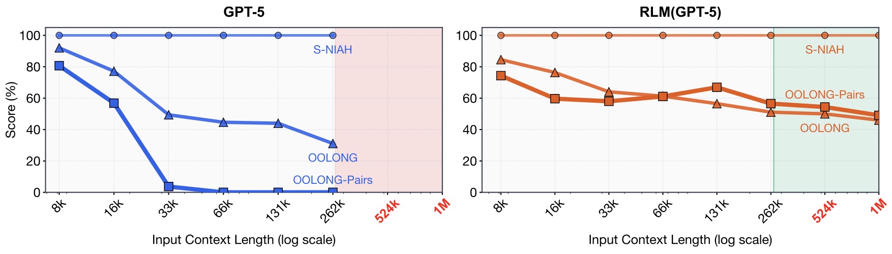
What recursion means here
-
“Recursive” in RLMs means the system can call language models as subroutines. The root model can inspect the external context, decide that part of the task should be solved locally, call a child model on that smaller subcontext, receive the child’s result, and continue.
-
A typical RLM trajectory has five phases:
- Inspect: The root model looks at the structure of the environment, such as document names, file paths, section headers, table schemas, or available helper functions.
- Search: It uses code, keyword search, metadata filters, or retrieval to find candidate regions.
- Delegate: It calls child models on coherent subcontexts, such as one paper, one function, one row batch, or one candidate pair.
- Aggregate: It combines child outputs with code, preserving IDs, offsets, spans, and other provenance.
- Finalize: It returns either a direct answer or an environment variable containing the answer, evidence, report, table, or artifact.
-
This is why the official alexzhang13/rlm repository describes RLMs as replacing a standard
llm.completion(prompt, model)call with anrlm.completion(prompt, model)call that offloads the context into a REPL environment and lets the model launch sub-LM calls over fragments. ([GitHub][3])
What RLMs are not
-
RLMs are not simply bigger prompts. The point is not to squeeze more text into the active model context; the point is to keep the full context outside the model and let the model control access to it.
-
RLMs are also not just retrieval-augmented generation. Retrieval usually selects top-\(k\) chunks and passes them to a model. An RLM can use retrieval, but it can also inspect metadata, expand around hits, recursively call children on full documents, verify claims, construct long artifacts, and store intermediate state.
-
RLMs are not the same as looped transformers. Looped transformers change the model architecture by reusing neural blocks inside a forward pass; RLMs change the inference scaffold by recursively calling models and manipulating external environment state. Scaling up Test-Time Compute with Latent Reasoning: A Recurrent Depth Approach by Geiping et al. (2025) studies recurrent latent computation inside the model, while Recursive Language Models by Zhang et al. (2025) studies recursive control over external context.
The key abstraction
-
An RLM can be described as a policy over environment actions:
\[a_t \sim \pi_\theta(a_t \mid q, h_t, E_t, b_t)\]- where \(q\) is the user query, \(h_t\) is the action-observation history, \(E_t\) is the current environment state, and \(b_t\) is the remaining budget.
-
The environment stores the long context and intermediate artifacts:
- The model’s active context no longer needs to contain the entire input. It only needs enough information to decide the next action:
- This is the central scaling move: replace “read everything in attention” with “control a computation over external state.”
Why RLMs are useful
-
RLMs are strongest when the task has natural substructure. Specifically:
- Long-context QA: Search for relevant regions, expand them into coherent passages, and answer from selected evidence.
- Evidence selection: Find exact supporting spans across many papers or documents.
- Dense aggregation: Classify many chunks or rows, then count or aggregate with code.
- Pairwise reasoning: Prune candidates before asking child models to judge pairs.
- Codebase analysis: Inspect file trees, search symbols, delegate to child models on relevant files, and preserve paths.
- Long report generation: Build sections as environment variables and return the final artifact with
FINAL_VAR. - Auditing and verification: Extract claims, check them against evidence, and report unsupported or inconsistent items.
-
The Reinforcing Recursive Language Models blog studies RL fine-tuning of 4B models to act as native RLMs, emphasizing that prompted RLMs are powerful but can have unpredictable latency and require careful prompt tuning. ([alphaXiv][5])
Practical takeaway
-
An RLM is best understood as a context controller:
- The model does semantic work: It interprets queries, chooses strategies, asks child models local questions, and synthesizes evidence.
- The environment does scalable work: It stores the full context, slices strings, searches files, counts rows, deduplicates spans, validates schemas, and preserves provenance.
- Recursive calls do local work: Children solve bounded subproblems instead of forcing the root to reason over the entire context at once.
- Finalization returns state: The answer can be a variable, table, evidence set, report, or structured artifact, not just prose emitted from memory.
-
RLMs are useful because they turn long-context reasoning into an explicit, inspectable computation. They scale not by increasing the model’s context window alone, but by giving the model a workspace and teaching it how to use that workspace.
Architecture
Runtime components
-
An RLM is built from five pieces:
- Root model: The controller. It receives the user query, sees the action-observation history, chooses what to inspect next, decides when to call children, and eventually finalizes the answer.
- Environment: The workspace. It stores the long prompt, helper functions, intermediate variables, child outputs, logs, and final artifacts.
- Action interface: The protocol by which the root model acts. In the canonical setup, actions are Python snippets executed in a REPL.
- Child-call interface: The mechanism that lets the root call the same model or another model on a smaller subcontext.
- Finalizer: The explicit stopping mechanism, such as
FINAL(answer)orFINAL_VAR("answer").
-
Recursive Language Models by Zhang et al. (2025) defines RLMs as a general inference strategy where the model programmatically examines an external prompt environment and recursively calls itself over snippets, while alexzhang13/rlm exposes this idea as a drop-in
rlm.completion(prompt, model)interface over a REPL-backed runtime.
Environment state
-
The environment is the main architectural difference between an RLM and a normal prompt. In a normal prompt, the model’s context window is the workspace. In an RLM, the workspace is external.
-
A useful environment contains:
- The original context: A string, document dictionary, file map, table, paper collection, transcript, or mixed structured object.
- Metadata: Titles, paths, section names, row IDs, offsets, timestamps, source URLs, or schema information.
- Helper functions: Search, preview, chunking, expansion, parsing, validation, deduplication, and formatting utilities.
- Intermediate variables: Candidate sets, evidence spans, child outputs, generated sections, verification verdicts, and final artifacts.
- Execution logs: Actions, observations, errors, child prompts, child outputs, costs, and finalization status.
-
The Recursive Language Models blog describes the concrete version of this architecture: the user prompt is stored as a variable inside a Python REPL, and the model interacts with that variable instead of receiving the whole context in its active prompt.
-
The following figure (source) shows the core RLM environment design: the long input prompt is placed inside a REPL environment as a variable, and the model writes code to inspect, decompose, and recursively call models over selected snippets.
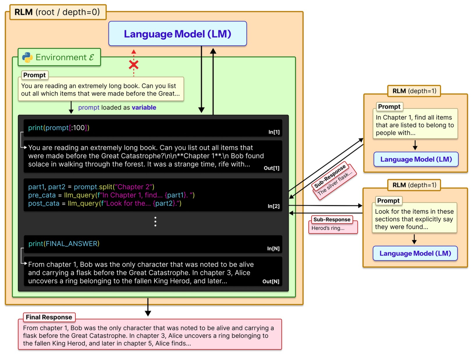
Control loop
-
At inference time, the RLM alternates between model actions and environment observations. The root model does not need to solve the whole task in one generation; it can use the environment to gather information, store results, and refine its plan.
-
A minimal architecture looks like:
env = PythonREPL({"context": long_context})

for step in range(max_steps):
    action = root_model.generate(query=query, history=env.history)
    observation = env.execute(action)
    env.history.append((action, observation))

    if is_final(action):
        return resolve_final(action, env)
- This makes the RLM closer to an agentic runtime than to a single LM call, but with a narrower objective: the central environment is the user-provided context itself. ReAct: Synergizing Reasoning and Acting in Language Models by Yao et al. (2022) introduced interleaved reasoning and acting over external environments, while RLMs specialize this idea for long-context processing with explicit prompt-as-environment state.
Child calls
-
Child calls are what make the architecture recursive. The root model can create a smaller task, bind it to a smaller subcontext, and ask a model to solve it locally.
-
A child call usually contains:
- A local instruction: For example, “extract exact evidence relevant to this claim” or “classify each row as yes/no.”
- A bounded subcontext: One section, file, row batch, paper, candidate pair, or retrieved passage group.
- A structured output request: JSON, a span list, a verdict, a table, or a short rationale.
- A provenance requirement: Document ID, file path, row ID, offset, section name, or source pointer.
-
The root model should not call children on arbitrary fragments. Good child calls are narrow enough to be cheap but complete enough to answer locally.
Finalization
-
RLMs need explicit finalization because the answer may live in the environment rather than in the root model’s latest text output.
-
Two common finalizers are:
FINAL(answer): Use this when the final response is short and can be safely emitted directly.FINAL_VAR("name"): Use this when the answer is stored in an environment variable, such as a report, evidence table, JSON object, or large artifact.
-
This matters because long answers, evidence sets, and generated reports should not be reconstructed from the root model’s limited active context. They should be returned from state.
Architectural invariant
- The central invariant is:
-
Instead, the active context contains only the query, instructions, recent observations, and compact environment summaries:
\[x_t = q \oplus s \oplus h_t \oplus \mathrm{summary}(E_t)\]- where \(q\) is the user query, \(s\) is the system or scaffold instruction, \(h_t\) is the trajectory history, and \(E_t\) is the external environment state.
-
This lets the full context be much larger:
- The model’s job is not to attend to all of \(E_t\). Its job is to choose useful actions over \(E_t\).
Design principles
-
A good RLM architecture follows a few practical rules:
- Keep the full context external: Do not repeatedly paste huge documents into model prompts.
- Expose natural structure: Preserve documents, sections, rows, files, functions, and metadata instead of flattening everything into one string.
- Use helpers for deterministic work: Search, slicing, counting, deduplication, validation, and formatting should be code, not prose reasoning.
- Use child calls for semantic work: Extraction, classification, comparison, and synthesis are the right jobs for model calls.
- Preserve provenance: Every evidence item should retain its source ID, offset, path, row ID, or section name.
- Cap observations: The root should see previews and summaries, while large variables remain in the environment.
- Make finalization explicit: Every successful run should end with a clear finalizer.
Practical takeaway
-
The architecture of an RLM is simple but powerful: a root model controls a workspace, the workspace stores the full context, helper functions manipulate that context, child calls solve bounded semantic subproblems, and finalizers return environment state.
-
This shifts the bottleneck from “Can the model fit the whole prompt?” to “Can the model choose a good computation over the prompt?”
Execution
Execution model
-
An RLM executes as a trajectory, not as a single completion. The root model repeatedly chooses an action, the environment executes it, and the resulting observation becomes part of the next decision. Recursive Language Models by Zhang et al. (2025) introduces this as an inference strategy where the model programmatically examines, decomposes, and recursively calls itself over snippets of an external prompt environment.
-
A trajectory can be written as:
\[\tau = (a_1, o_1, a_2, o_2, \ldots, a_T, o_T, y)\]- where \(a_t\) is the root model’s action, \(o_t\) is the environment observation, and \(y\) is the final answer or returned environment variable.
-
A minimal loop is:
for step in range(max_steps):
    action = root_model(query, history, budget)
    observation = env.execute(action)
    history.append((action, observation))

    if is_final(action):
        return resolve_final(action, env)
Action types
-
The root model’s actions are usually code snippets. Executable Code Actions Elicit Better LLM Agents by Wang et al. (2024) motivates executable code as a flexible action space for LLM agents, and RLMs use that idea specifically for long-context control.
-
Common RLM actions include:
- Inspect: Look at document titles, file paths, section headers, table schemas, row counts, or available helper functions.
- Search: Run keyword, regex, metadata, vector, or hybrid search over the external context.
- Expand: Turn a hit snippet into a coherent paragraph, section, function, row group, or document window.
- Delegate: Send a bounded subcontext to a child model with a local instruction.
- Aggregate: Parse child outputs, deduplicate evidence, count rows, merge tables, or synthesize claims.
- Verify: Check support, schema validity, arithmetic, contradictions, or coverage.
- Finalize: Return a direct answer or an environment variable.
-
The action space should make good behavior easy: helpers should preserve provenance, cap outputs, validate schemas, and warn when an operation would exceed budget.
Inspect
-
Execution usually begins with inspection. The root should understand the shape of the context before choosing a strategy.
-
For different contexts, inspection means different things:
- Document corpus: List titles, abstracts, dates, sources, sections, and metadata.
- Codebase: List directories, file paths, imports, class names, function names, and tests.
- Table: Inspect columns, row count, missing values, key fields, and candidate grouping columns.
- Transcript: Inspect speakers, timestamps, sections, and repeated entities.
- Research packet: Inspect paper titles, authors, abstracts, figures, and references.
-
The goal is to choose the right decomposition before spending compute. A sparse lookup task may need only search and expansion; a dense aggregation task may need map-reduce; a pairwise reasoning task may need pruning before pair construction.
Search
-
Search converts a huge context into a candidate set. Recursive Language Models describes the RLM setup as storing the prompt in a REPL variable so the model can interact with it programmatically, which makes search and slicing first-class runtime operations. ([Alex L. Zhang][3])
-
A good search phase uses multiple signals:
- Exact anchors: Names, dates, file paths, method names, benchmark names, IDs, symbols, and quoted phrases.
- Paraphrases: Synonyms, abbreviations, related terms, and alternate terminology.
- Metadata: Titles, headings, source fields, row labels, file names, and section names.
- Fallbacks: Broader searches, chunk sweeps, retrieval, or structural traversal when exact search fails.
-
Search should produce candidates, not final answers. The root should expand hits into coherent local context before calling children or synthesizing.
Decompose
-
Decomposition is the central execution decision. The root model chooses how to break the task into local subproblems.
-
Useful decomposition units include:
- By document: Send each relevant paper, report, email, or web page to a child model.
- By section: Use sections when a full document is too large or topically diverse.
- By file or function: Use files and symbols for codebase reasoning.
- By row batch: Use row groups for table classification or data cleaning.
- By candidate pair: Use pruned pairs for duplicate detection, contradiction checks, or entity linking.
- By claim: Use extracted claims for audit and verification workflows.
-
Good decomposition has two properties:
- Local answerability: Each child call has enough context to solve its subproblem without global state.
- Bounded cost: Each child call is small enough to be cheap, fast, and reliable.
Delegate
-
Delegation is where recursion enters. The root model calls a model on a bounded subcontext and receives a local result.
-
A good child call contains:
- A narrow instruction: Ask for extraction, classification, comparison, or verification, not a vague summary.
- A coherent subcontext: Send a whole paragraph, section, file, row batch, or candidate pair.
- A structured output format: Prefer JSON, lists of spans, verdicts, labels, or tables over free-form prose.
- A provenance requirement: Preserve document ID, file path, row ID, section name, offset, or source span.
-
For example, an evidence-selection child call should ask for exact supporting spans, not a general explanation. A row-classification child call should return row IDs and labels, not a paragraph summary.
Aggregate
-
Aggregation turns local child outputs into a global result. This is where RLMs should rely heavily on code.
-
Aggregation should handle:
- Parsing: Convert child outputs into typed objects.
- Deduplication: Remove repeated spans, rows, files, or claims.
- Counting: Compute totals deterministically rather than asking the model to count from prose.
- Merging: Combine partial tables, evidence sets, or section drafts.
- Ranking: Sort evidence by relevance, confidence, source quality, or coverage.
- Provenance preservation: Keep source IDs attached to every claim or item.
-
The important split is:
- Models do semantic work: classify, extract, compare, explain, synthesize.
- Code does deterministic work: count, sort, validate, deduplicate, merge, format.
-
This split makes the final result easier to audit and less likely to contain arithmetic or provenance errors.
Verify
-
Verification is most useful after aggregation. It should check the selected evidence and structured outputs, not reread the entire context.
-
Useful verification checks include:
- Support: Every final claim is backed by selected evidence.
- Completeness: The answer covers all parts of the user query.
- Contradiction: No selected evidence contradicts the answer.
- Schema validity: The final object matches the required format.
- Arithmetic: Counts and totals match the underlying records.
- Minimality: Evidence spans are concise and directly relevant.
-
ReAct: Synergizing Reasoning and Acting in Language Models by Yao et al. (2022) shows the value of interleaving reasoning with environment actions, and RLM verification is a specialized form of that loop: the system acts on context, observes evidence, and revises or finalizes based on grounded checks.
Stop
-
Stopping is an execution skill. The root model should stop once the environment contains a sufficiently supported answer.
-
A good stopping rule considers:
- Evidence sufficiency: Enough relevant evidence has been found to answer the query.
- Coverage: All query parts have been addressed.
- Budget: Further recursion is unlikely to improve the result enough to justify cost.
- Verification: The answer passes support, schema, and arithmetic checks.
- Finalization form: The answer is available directly or stored in a variable ready for return.
-
The finalizer should be explicit:
- Use
FINAL(answer)for short answers that can be emitted directly. - Use
FINAL_VAR("answer")for reports, evidence sets, tables, JSON artifacts, or long outputs stored in the environment.
- Use
Execution failures
-
RLMs fail when the trajectory is bad, even if the base model is strong.
-
Common failures include:
- Poor inspection: The root never understands the structure of the context.
- Bad search terms: Relevant regions are missed because the query terms are too narrow or lexical.
- Bad chunking: Children receive fragments that are too small, too large, or cut across natural boundaries.
- Over-recursion: The root calls children on too many low-value units.
- Under-recursion: The root tries to solve semantic tasks with brittle keyword search alone.
- Observation flooding: The root prints huge variables and pollutes its active context.
- Unsupported aggregation: The final answer adds claims not present in selected evidence.
- Weak finalization: The root emits prose from memory instead of returning the environment variable that contains the grounded result.
Practical takeaway
-
RLM execution is disciplined context control. The root model should inspect structure, search broadly enough for recall, decompose into locally answerable subproblems, delegate semantic work, aggregate with code, verify selected evidence, and stop explicitly.
-
The strongest RLM trajectories are not the longest ones. They are the trajectories that spend compute where it changes the answer.
Patterns
Search and expand
-
Search-and-expand is the most basic RLM pattern. The root model first searches the external context for candidate regions, then expands each hit into a coherent local unit before reasoning over it. Recursive Language Models by Zhang et al. (2025) motivates this pattern by treating the prompt as external state that the model can inspect and decompose programmatically.
-
The pattern is:
- Search broadly enough for recall: Use exact names, paraphrases, headings, metadata fields, symbols, and related terms.
- Expand around hits: Convert a short match into a paragraph, section, table slice, function body, or document window.
- Preserve provenance: Every expanded unit should keep source ID, offset, section name, file path, row range, or title.
- Reason only after expansion: A raw hit snippet is often too narrow; the child model should receive enough context to answer locally.
-
A compact implementation sketch:
hits = search(context, query_terms)
units = [expand_hit(hit, by="section") for hit in hits[:k]]
evidence = ask_children("Extract directly relevant evidence.", units)
answer = synthesize(query, evidence)
- Use this pattern for long-context QA, source-backed answers, code search, research packets, and evidence selection.
Map reduce
-
Map-reduce is the default pattern when many independent units need local semantic analysis followed by deterministic aggregation. Oolong: Evaluating Long Context Reasoning and Aggregation Capabilities by Bertsch et al. (2025) is especially relevant because it evaluates tasks where models must classify or reason over many chunks and aggregate the results, rather than retrieve one answer-bearing span.
-
The pattern is:
- Map: Apply the same local instruction to many units, such as documents, sections, rows, claims, files, or examples.
- Structure child outputs: Require JSON, labels, row IDs, evidence spans, verdicts, or short normalized fields.
- Reduce with code: Count, deduplicate, group, sort, validate, and merge deterministically.
- Synthesize last: Use the model only after structured evidence or aggregate values have been computed.
-
This division of labor is important:
- Model calls handle semantics: classification, extraction, comparison, explanation, and summarization.
- Code handles arithmetic and state: counting, joining, validating, deduplicating, and formatting.
- The environment preserves provenance: source IDs, row IDs, offsets, paths, and spans stay attached to outputs.
-
Use this pattern for dense aggregation, survey analysis, claim audits, long transcript analysis, row classification, and multi-document summaries.
Evidence selection
-
Evidence selection is a specialized RLM pattern where the final product is not just an answer, but a set of supporting spans. The Reinforcing Recursive Language Models blog studies native RLM training on evidence selection over scientific documents, where a shared parent-child policy learns to dispatch itself onto subproblems and extract relevant evidence.
-
The pattern is:
- Triage sources: The root model first ranks papers, documents, files, or sections by relevance.
- Delegate extraction: Child calls receive bounded source units and return exact spans or structured evidence objects.
- Validate spans: The environment checks that extracted text appears in the source and keeps offsets or source pointers.
- Aggregate minimally: The final evidence set should be sufficient but not bloated with irrelevant passages.
- Answer from evidence: Synthesis should happen only after evidence has been selected and checked.
-
A useful evidence object is:
{
  "source_id": "paper_03",
  "section": "Training",
  "span": "...",
  "reason": "Supports the claim about recursive child rollouts."
}
- Use this pattern when users ask for grounded research answers, literature reviews, compliance checks, citation-backed summaries, or claim verification.
Prune then pair
- Pairwise reasoning is expensive because the number of candidate pairs grows quadratically:
-
An RLM should therefore prune before asking child models to judge pairs. This is central for duplicate detection, contradiction detection, entity linking, clue matching, and cross-document comparison.
-
The pattern is:
- Generate candidates: Use search, metadata, embeddings, or cheap rules to create a candidate set.
- Prune aggressively: Reduce \(n\) to a much smaller \(k\) before constructing pairs.
- Construct plausible pairs only: Use shared entities, dates, symbols, file paths, labels, or similarity thresholds.
- Delegate pair judgments: Ask child models local yes/no or relation-classification questions.
- Aggregate with thresholds: Use code to merge positive pairs, deduplicate edges, or form clusters.
-
The effective goal is:
- Use this pattern for OOLONG-Pairs-style workloads, entity resolution, code-change dependency checks, contradiction graphs, and matching tasks.
Retrieve then reason
-
RLMs can wrap retrieval systems rather than replace them. Retrieval supplies candidate chunks; the RLM expands, verifies, recursively delegates, and synthesizes. From Local to Global: A Graph RAG Approach to Query-Focused Summarization by Edge et al. (2024) is relevant because it structures retrieval around graph communities and summaries, while an RLM can dynamically operate over retrieved structures through an executable environment. ([Microsoft GitHub][3])
-
The pattern is:
- Retrieve candidates: Use vector search, keyword search, graph search, metadata search, or hybrid retrieval.
- Expand retrieved chunks: Pull neighboring sections, full documents, linked nodes, or table rows.
- Rerank with the root: Filter candidates by direct relevance to the query.
- Delegate local extraction: Ask children to extract evidence or answer local subquestions.
- Verify before final synthesis: Check that final claims are supported by selected retrieved evidence.
-
This pattern is useful when the corpus is large or persistent, but retrieval alone is too shallow for the question.
Codebase traversal
-
Codebases are naturally suited to RLMs because they already have structure: directories, files, symbols, imports, tests, and call graphs. SWE-bench: Can Language Models Resolve Real-World GitHub Issues? by Jimenez et al. (2023) is relevant because repository-level issue solving requires understanding and coordinating changes across multiple files.
-
The pattern is:
- Inspect the tree: List files, directories, tests, configuration files, and package boundaries.
- Search symbols: Find functions, classes, imports, error messages, API names, and test failures.
- Extract coherent units: Use files, functions, classes, or test cases rather than arbitrary text chunks.
- Delegate local analysis: Ask child models to explain whether each unit is relevant to the issue.
- Aggregate by dependency: Connect findings across files, imports, call sites, tests, and expected behavior.
- Return paths and patches: Preserve file paths and line-level provenance wherever possible.
-
Use this pattern for bug localization, repository Q&A, migration planning, dependency audits, test failure analysis, and patch planning.
Build and return
-
Some tasks require producing a long artifact: a report, evidence table, JSON file, migration plan, audit result, or generated document. In an RLM, the artifact should live in the environment rather than in the root model’s active context.
-
The pattern is:
- Create sections or records incrementally: Build the artifact piece by piece.
- Store intermediate state: Keep drafts, evidence tables, and generated sections as variables.
- Preview selectively: Print only short previews or summaries, not the entire artifact.
- Revise locally: Edit one section, row group, or field without regenerating everything.
- Return by variable: Use
FINAL_VAR("artifact")for long outputs.
-
This pattern is especially useful for long reports, structured exports, evidence packets, data-cleaning outputs, and multi-section primers.
Verify and repair
-
Verification is a reusable pattern, not just a final step. The root model can use verification whenever an intermediate or final result may be unsupported, malformed, incomplete, or inconsistent.
-
The pattern is:
- Check support: Every major claim should map to selected evidence.
- Check completeness: Every part of the user query should be addressed.
- Check contradictions: Conflicting evidence should be surfaced, not hidden.
- Check schemas: JSON, tables, citations, row IDs, and required fields should validate.
- Check arithmetic: Counts, totals, and percentages should be recomputed by code.
- Repair narrowly: Rerun only the missing search, malformed child call, or unsupported section.
-
Verification should inspect the selected evidence and structured outputs, not restart the entire task. This keeps cost bounded and makes failures easier to debug.
Pattern selection
- RLMs are most effective when the root model chooses a pattern that matches the task shape.
| Task shape | Recommended pattern |
|---|---|
| One or a few relevant passages | Search and expand |
| Many independent units | Map reduce |
| Need exact supporting spans | Evidence selection |
| Relations between items | Prune then pair |
| Large indexed corpus | Retrieve then reason |
| Repository or codebase | Codebase traversal |
| Long output artifact | Build and return |
| High risk of unsupported claims | Verify and repair |
-
The practical rule is:
- Use search when relevance is sparse.
- Use map-reduce when work is distributed across many units.
- Use pruning when pairwise reasoning would explode.
- Use retrieval when the corpus is too large for direct environment scanning.
- Use variables when the output is long or structured.
- Use verification when the answer must be grounded.
Practical takeaway
-
RLM patterns are recipes for controlling context. The model should not merely “think longer”; it should choose the right computation over external state.
-
The core patterns are search, map, reduce, delegate, verify, and return. Their value comes from combining semantic model calls with deterministic environment operations while preserving provenance throughout the trajectory.
Training
Training objective
-
Training an RLM means training a model to control a context environment, not just to emit an answer. The model must learn when to inspect, search, decompose, call children, aggregate, verify, and stop. Recursive Language Models by Zhang et al. (2025) defines the RLM setting as inference over an external prompt environment, while Reinforcing Recursive Language Models studies how small models can be RL fine-tuned to behave as native RLM controllers.
-
The policy can be written as:
\[\pi_\theta(a_t \mid q, h_t, E_t, b_t)\]- where \(a_t\) is the next action, \(q\) is the query, \(h_t\) is the action-observation history, \(E_t\) is the environment state, and \(b_t\) is the remaining budget.
-
The training target is a trajectory:
\[\tau = (a_1, o_1, a_2, o_2, \ldots, a_T, o_T, y)\]- not just a final answer \(y\).
What the model must learn
-
A useful RLM policy needs four skills:
- Protocol fluency: It must use the scaffold correctly: call helper functions, parse observations, handle errors, use child-call primitives, and finish with
FINALorFINAL_VAR. - Decomposition strategy: It must choose between search-and-expand, map-reduce, evidence selection, prune-then-pair, retrieval-then-reason, or build-and-return based on task shape.
- Budget discipline: It must avoid excessive child calls, huge printed observations, repeated verification loops, and unnecessary recursion.
- Faithful aggregation: It must preserve provenance, deduplicate evidence, avoid unsupported synthesis, and return the environment variable that actually contains the grounded result.
- Protocol fluency: It must use the scaffold correctly: call helper functions, parse observations, handle errors, use child-call primitives, and finish with
-
This is why prompted RLMs can be powerful but brittle: a general model may understand the prompt, yet still over-search, under-search, recurse at the wrong granularity, or fail to stop. Reinforcing Recursive Language Models frames RL fine-tuning as a way to make these control behaviors reliable in smaller, cheaper models.
Training data
-
RLM training data should contain trajectories, not only input-output pairs.
-
Each training example should record:
- Task input: Query, context ID, context type, available helpers, and budget.
- Root actions: Code snippets, searches, child-call decisions, aggregation steps, and finalizer.
- Observations: Search results, previews, errors, parsed objects, child outputs, and verification results.
- Child trajectories: Prompts, subcontexts, actions, outputs, and local finalization.
- Final result: Answer, evidence set, table, report, or artifact.
- Scores: Task reward, evidence reward, format reward, cost, latency, and failure flags.
-
A compact trace representation is:
{
  "query": "...",
  "context_id": "...",
  "actions": ["inspect()", "hits = search(...)", "evidence = rlm_query_batched(...)"],
  "observations": ["...", "..."],
  "finalizer": "FINAL_VAR('evidence')",
  "reward": 0.82,
  "cost": {"root_steps": 5, "child_calls": 12}
}
- For evidence-selection workloads, the final target can be a list of source-grounded spans rather than a prose answer. Reinforcing Recursive Language Models uses scientific evidence selection as its main setting, because it forces the model to learn source triage, child delegation, span extraction, and aggregation. ([alphaXiv][2])
Supervised warm start
-
A small RLM usually needs supervised fine-tuning before RL. SFT teaches the scaffold syntax and common trajectories, while RL later teaches which trajectories are actually good.
-
SFT should emphasize:
- Clean protocol examples: Correct use of helpers, child calls, JSON outputs, and finalizers.
- Short successful traces: Compact trajectories that solve the task without unnecessary recursion.
- Representative task shapes: Search, aggregation, evidence selection, verification, and long-output return.
- Error recovery examples: Handling empty searches, malformed child outputs, parsing failures, and budget warnings.
-
The supervised objective is ordinary next-token prediction over action traces:
\[\mathcal{L}_{\mathrm{SFT}}(\theta) =-\sum_{t=1}^{T} \sum_{j=1}^{|a_t|} \log \pi_\theta(a_{t,j} \mid x_t, a_{t,<j})\]- where \(x_t\) is the formatted state at step \(t\) and \(a_t\) is the target action.
-
SFT is useful, but it can also overfit teacher behavior. If teacher traces are verbose, expensive, or overly template-driven, the student may learn bad RLM habits. The goal is not to imitate every trace; it is to learn the protocol and a few robust starting strategies.
Reinforcement learning
-
RL is useful because many RLM decisions are strategic rather than syntactic. The model may have several valid trajectories, but only some are cheap, grounded, and robust.
-
A reward can combine task quality and trajectory quality:
\[R(\tau) =R_{\mathrm{task}} + R_{\mathrm{grounding}} + R_{\mathrm{format}} - \lambda_1 C - \lambda_2 L - \lambda_3 M - \lambda_4 O\]- where \(C\) is token or dollar cost, \(L\) is latency, \(M\) is number of child calls, and \(O\) is observation volume.
-
Useful reward components include:
- Task reward: Exact match, accuracy, rubric score, or evidence F1.
- Grounding reward: Claims are supported by selected evidence.
- Format reward: Output schema and finalizer are valid.
- Cost penalty: Child calls, large prompts, retries, and long observations are penalized.
- Latency penalty: Serial recursion and slow child calls are discouraged.
- Failure penalty: Timeouts, invalid JSON, unsafe actions, or missing finalization receive low reward.
-
Proximal Policy Optimization Algorithms by Schulman et al. (2017) introduced PPO as a clipped policy-gradient method for stable RL updates, and DeepSeekMath: Pushing the Limits of Mathematical Reasoning in Open Language Models by Shao et al. (2024) introduced GRPO as a critic-free PPO variant that compares grouped rollouts and is now commonly used for LLM reasoning RL.
GRPO-style training
-
Group Relative Policy Optimization is natural for RLMs because the same task can be solved by multiple sampled trajectories. Instead of needing an external value model, the system compares rollouts within a group.
-
For a task \(x\), sample \(G\) trajectories:
- Score each trajectory:
- Compute group-relative advantages:
-
Then update the policy with a clipped objective:
\[\mathcal{L}_{\mathrm{GRPO}}(\theta) =\mathbb{E}_{g,t} \left[ \min \left( \rho_{g,t} A_g, \mathrm{clip}(\rho_{g,t}, 1-\epsilon, 1+\epsilon) A_g \right) \right] -\beta D_{\mathrm{KL}}(\pi_\theta | \pi_{\mathrm{ref}})\]-
where:
\[\rho_{g,t} =\frac{ \pi_\theta(a_{g,t} \mid x_{g,t}) }{ \pi_{\theta_{\mathrm{old}}}(a_{g,t} \mid x_{g,t}) }\]
-
-
This objective rewards trajectories that outperform other attempts on the same task, while the KL term prevents the policy from drifting too far from the reference model. DeepSeekMath by Shao et al. (2024) uses GRPO to improve mathematical reasoning while reducing PPO memory overhead from a separate critic.
Shared parent-child policy
- A native RLM can use one model for both parent and child roles:
-
This matters because recursive calls are not a separate system; they are the same policy operating at a smaller scope.
-
The shared-policy setup has three benefits:
- Unified behavior: The same model learns both how to decompose and how to solve decomposed tasks.
- More training signal: Child traces become training data for the same policy that controls the root.
- Simpler deployment: One fine-tuned model can act as planner, extractor, verifier, and local solver.
-
The main credit-assignment challenge is that child rollouts may not have their own direct reward. Reinforcing Recursive Language Models addresses this by letting child rollouts inherit the advantage of the parent rollout that spawned them, eliminating the need for separate child-specific reward signals. ([alphaXiv][2])
Training stability
-
RLM training is sensitive because the model is learning a policy over tools, state, recursion, and budgets.
-
Common stability problems include:
- Reward sparsity: The system may only know whether the final answer was good after many actions and child calls.
- Bad credit assignment: A strong final answer may depend on one useful search, one good child call, or one correct aggregation step.
- Child-gradient imbalance: If each parent spawns many children, child traces can dominate training unless normalized.
- Prompt dependence: The model may learn to rely on long strategy prompts instead of internalizing control behavior.
- Cost hacking: The model may avoid useful child calls to reduce cost penalties.
- Format hacking: The model may optimize for valid-looking outputs without improving evidence quality.
- Exploration collapse: Heavy SFT can make the policy too deterministic before RL.
-
Practical stabilizers include:
- Start with small, clean SFT: Teach protocol without overfitting long teacher traces.
- Use grouped rollouts: Compare multiple trajectories for the same task.
- Normalize child losses: Prevent high-fanout trees from overwhelming the parent signal.
- Track KL and entropy: Detect policy collapse or excessive drift.
- Separate quality and cost metrics: Ensure reward gains are not just cheap but worse behavior.
- Evaluate held-out trajectories: Inspect whether the model learned better decomposition, not merely better formatting.
Evaluation during training
-
Training should monitor both outcome quality and trajectory behavior.
-
Outcome metrics:
- Answer accuracy: Exact match, classification accuracy, rubric score, or task success.
- Evidence quality: Precision, recall, span F1, support score, or judge score.
- Faithfulness: Whether final claims are supported by selected evidence.
- Completeness: Whether all query parts are answered.
-
Trajectory metrics:
- Root steps: Number of model-environment turns.
- Child calls: Total recursive calls and call fanout.
- Observation volume: Amount of text printed back into the root context.
- Latency: Median and tail latency.
- Cost: Token cost, model-call cost, and retry cost.
- Failure rate: Timeouts, invalid finalizers, malformed JSON, sandbox errors, and missing provenance.
-
A model is improving as an RLM only if quality rises without uncontrolled growth in cost, child calls, or latency.
Practical takeaway
- Training RLMs is about learning recursive control. SFT teaches the model the scaffold; RL teaches it which scaffold actions are useful. The best trained RLMs do not simply call themselves more often. They learn to search selectively, decompose coherently, call children only when semantics require it, aggregate with code, preserve evidence, verify when needed, and stop once the answer is sufficiently supported.
Evaluation
What to evaluate
-
RLM evaluation should measure the quality of a computation, not only the quality of a final answer. A direct long-context model is evaluated on whether it answers correctly after receiving a prompt. An RLM must also be evaluated on whether it chose a good trajectory through an external environment. Recursive Language Models by Zhang et al. (2025) evaluates RLMs as systems that inspect, decompose, and recursively process external prompt state rather than as single-pass readers.
-
The evaluation object is:
\[\tau = (a_1, o_1, a_2, o_2, \ldots, a_T, o_T, y)\]- where \(\tau\) is the full trajectory, \(a_t\) are actions, \(o_t\) are observations, and \(y\) is the final answer or returned environment variable.
-
A complete evaluation should ask:
- Answer quality: Did the system produce the right answer, evidence set, table, report, or artifact?
- Evidence quality: Did it identify the right supporting spans, preserve provenance, and avoid unsupported claims?
- Trajectory quality: Did it inspect the right structure, search effectively, decompose coherently, and aggregate faithfully?
- Efficiency: Did it achieve the result within acceptable cost, latency, child-call count, and observation budget?
- Robustness: Did it handle distractors, paraphrases, noisy formatting, missing evidence, and tighter budgets gracefully?
Task axes
-
RLMs should be tested across multiple task axes because long-context performance is not one capability.
-
Important axes include:
- Length: How performance changes from thousands to millions of tokens.
- Density: Whether the answer depends on one passage, many passages, or most of the context.
- Structure: Whether the input is a document, codebase, table, transcript, paper collection, or mixed corpus.
- Reasoning type: Retrieval, multi-hop synthesis, aggregation, pairwise comparison, evidence selection, or report construction.
- Decomposition difficulty: Whether the task naturally splits into independent local subproblems or requires careful global planning.
- Budget pressure: Whether the system can maintain quality under limits on child calls, latency, observation size, or cost.
-
RULER: What’s the Real Context Size of Your Long-Context Language Models? by Hsieh et al. (2024) is useful here because it shows that simple needle retrieval is not enough: long-context evaluations should include multi-hop tracing and aggregation tasks that become harder as length and task complexity increase.
Benchmark families
-
A strong RLM benchmark suite should include both long-context benchmarks and RLM-specific trajectory evaluations.
-
Useful benchmark families include:
- Needle-style retrieval: Tests whether the system can locate a small amount of relevant information in a large context.
- Multi-hop long-context QA: Tests whether the system can combine evidence across multiple regions.
- Dense aggregation: Tests whether the system can classify many units and aggregate results.
- Pairwise reasoning: Tests whether the system can prune and compare candidate pairs without quadratic blowup.
- Evidence selection: Tests whether the system can return exact supporting spans rather than only prose answers.
- Codebase tasks: Tests whether the system can inspect files, locate relevant symbols, and preserve paths.
- Long-output tasks: Tests whether the system can build reports, tables, JSON artifacts, or evidence packets in environment state.
-
Oolong: Evaluating Long Context Reasoning and Aggregation Capabilities by Bertsch et al. (2025) is especially relevant for RLMs because it evaluates classification, counting, temporal reasoning, and aggregation over many context chunks, not just retrieval from a few passages.
Answer metrics
-
Answer metrics depend on task type.
-
For exact-answer tasks:
- For evidence-selection tasks, span-level precision, recall, and \(F_1\) are more informative:
-
For generated reports or research answers, rubric-based evaluation is often needed.
-
Useful rubric dimensions include:
- Correctness: The answer is factually right.
- Grounding: Major claims are supported by selected evidence.
- Completeness: All parts of the query are addressed.
- Specificity: The answer avoids vague synthesis when exact spans or values are available.
- Contradiction handling: Conflicting evidence is acknowledged rather than hidden.
- Format validity: The output matches the requested schema, table, citation, or artifact format.
-
LongBench v2 evaluates long-context understanding across realistic tasks with long inputs and deeper reasoning requirements, making it useful for testing answer quality beyond simple retrieval.
Trajectory metrics
-
RLMs need trajectory metrics because two systems can produce the same answer with very different cost, latency, and reliability.
-
Key trajectory metrics include:
- Root steps: Number of environment actions before finalization.
- Child calls: Total recursive calls and fanout per step.
- Observation volume: Number of characters or tokens printed back to the root.
- Child prompt volume: Total tokens sent into child calls.
- Latency: Median, p95, and p99 wall-clock time.
- Cost: Model-call cost, token cost, tool cost, and retry cost.
- Failure rate: Timeouts, invalid finalizers, malformed child outputs, sandbox errors, and budget exhaustion.
- Grounding rate: Fraction of final claims linked to selected evidence.
- Provenance coverage: Fraction of evidence items with source IDs, offsets, row IDs, file paths, or section names.
-
A useful utility score is:
\[U=Q - \lambda C - \mu L - \nu F\]- where \(Q\) is quality, \(C\) is cost, \(L\) is latency, and \(F\) is failure rate.
Baselines
-
RLMs should be compared against both model-only and scaffolded baselines.
-
Important baselines include:
- Direct long-context model: Put as much of the context as possible into the model window and answer directly.
- Truncation baseline: Use prefix, suffix, middle, or heuristic context selection when the input is too long.
- Retrieval baseline: Retrieve top-\(k\) chunks and answer from them.
- Summarization baseline: Summarize chunks first, then answer from the summaries.
- ReAct-style agent: Let the model interleave reasoning and tool use without the full RLM prompt-as-environment design.
- RLM without child calls: Keep the REPL and helpers but disable recursion.
- RLM without helpers: Allow child calls but remove high-quality search, chunking, and validation helpers.
- RLM without verification: Measure how much support-checking and repair improve reliability.
-
These baselines isolate which part of the RLM matters: external memory, helper functions, recursive calls, child batching, or verification.
Scaling curves
-
RLM evaluation should include scaling curves over context length and task complexity. Recursive Language Models by Zhang et al. (2025) reports that RLMs remain effective at lengths where direct models degrade or exceed their context windows, making scaling curves central to the evaluation story.
-
Measure:
\[Q(N), \quad C(N), \quad L(N), \quad F(N)\]- where \(N\) is context length, \(Q\) is quality, \(C\) is cost, \(L\) is latency, and \(F\) is failure rate.
-
Scaling should vary:
- Input length: From short contexts to contexts beyond the base model window.
- Task density: From one relevant passage to many relevant units.
- Fanout pressure: From a few child calls to many possible subproblems.
- Pairwise complexity: From linear processing to pruned pairwise reasoning.
- Output length: From short answers to long reports or structured artifacts.
-
The goal is not only to show that quality remains high. The goal is to show that cost and latency remain controlled.
Ablations
-
Ablations reveal whether the RLM is actually using recursive context control.
-
Useful ablations include:
- No recursion: Disable child calls and test whether REPL-only search is enough.
- No search helpers: Force the model to use raw context inspection and see whether performance collapses.
- No structured outputs: Let children return prose instead of JSON, spans, labels, or verdicts.
- No provenance: Remove source IDs or offsets and measure grounding loss.
- No verification: Skip support and schema checks.
- Smaller child-call budget: Vary maximum child calls, such as \(M \in {0, 4, 16, 64}\).
- Smaller observation budget: Test whether the root relies on flooding itself with printed text.
- Different root-child model assignments: Swap strong and weak models between planner and local solver roles.
-
A good ablation suite should answer:
- Is recursion helping?
- Are helpers helping?
- Is verification helping?
- Is the model decomposing intelligently?
- Is the system robust under tighter budgets?
Robustness tests
-
RLMs can overfit to formatting, helper names, document order, or easy lexical anchors. Robustness tests should perturb the environment while keeping the underlying answer unchanged.
-
Useful perturbations include:
- Document shuffling: Reorder documents, rows, files, or sections.
- Distractor injection: Add near-miss passages that contain query terms but do not answer the question.
- Lexical paraphrase: Rewrite the query to remove obvious anchor terms.
- Format variation: Change headings, separators, schema labels, or file organization.
- Noisy text: Add OCR errors, duplicated paragraphs, malformed tables, or broken JSON.
- Hard negatives: Include sources that look relevant but contradict the answer.
- Budget tightening: Reduce steps, child calls, or observation size.
-
The purpose is to test whether the RLM learned robust context control or merely learned brittle search recipes.
Diagnostics
-
Every RLM evaluation should include trajectory diagnostics. A wrong answer should be assigned to a failure stage.
-
Diagnostic categories include:
- Inspection failure: The root did not understand the context structure.
- Search failure: Relevant regions were never retrieved or expanded.
- Chunking failure: Children received incomplete or oversized subcontexts.
- Delegation failure: Child prompts were vague, too broad, or locally unanswerable.
- Aggregation failure: Correct child outputs were dropped, duplicated, or miscounted.
- Verification failure: Unsupported claims were not caught.
- Finalization failure: The answer variable existed but the root returned the wrong output.
- Budget failure: The trajectory exhausted time, steps, calls, or observation limits.
-
A compact diagnostic record might store:
{
  "stage": "aggregation",
  "root_steps": 7,
  "child_calls": 24,
  "failure": "duplicate evidence counted twice",
  "finalizer": "FINAL_VAR('answer')"
}
- This makes evaluation actionable: developers can improve the stage that failed instead of only seeing a lower score.
Reporting
-
A good RLM report should present quality and systems behavior together, rather than putting all methods behind one headline score. Specifics below:
- Compare methods across the same quality and efficiency dimensions: For each direct model, retrieval baseline, summarization baseline, ReAct-style scaffold, RLM ablation, and full RLM, report answer quality, evidence support, cost, median latency, tail latency, child-call count, and failure rate. This makes it clear whether an RLM is winning because it is more accurate, because it is cheaper, because it is better grounded, or because it has a better quality-cost tradeoff.
- Break results down by task family and context regime: Sparse retrieval, dense aggregation, pairwise reasoning, codebase reasoning, evidence selection, and long-output generation should not be averaged into one undifferentiated number. They stress different parts of the system: search, decomposition, recursion, aggregation, verification, and finalization.
Practical takeaway
-
RLM evaluation should answer three questions:
- Quality: Did the system produce the right answer or evidence?
- Control: Did it choose a scalable trajectory through the context?
- Efficiency: Did it achieve quality within acceptable cost, latency, and failure limits?
-
The best RLM is not the one that recurses the most. It is the one that uses recursion only when it improves grounded, efficient context processing.
Use Cases
When RLMs are most useful
-
RLMs are most useful when the context is large, structured, and decomposable. The goal is not merely to answer from a long prompt, but to control a computation over that prompt. Recursive Language Models by Zhang et al. (2025) presents RLMs as an inference strategy for processing arbitrarily long prompts by storing the prompt externally and letting the model inspect, decompose, and recursively process selected snippets.
-
Good RLM use cases usually share three properties:
- The context is too large or noisy for direct prompting: The input may contain many documents, files, rows, papers, logs, messages, or transcript segments.
- The task has natural subproblems: The system can split work by document, section, row batch, file, function, claim, or candidate pair.
- The final answer benefits from provenance: The output should preserve evidence spans, file paths, row IDs, source documents, offsets, or intermediate artifacts.
Long-context QA
-
Long-context QA is the most direct RLM use case. Instead of putting the whole context into the prompt, the root model searches the environment, expands relevant hits, asks child models local questions, and synthesizes a grounded answer.
-
This is useful for:
- Large document packets: Legal records, research packets, policy manuals, technical documentation, or archives.
- Mixed-source questions: Queries that require comparing facts across multiple reports, pages, or sections.
- Sparse evidence tasks: Cases where only a few passages matter, but they are buried in a large corpus.
- Context-rot mitigation: Cases where direct long-context prompting degrades as irrelevant text accumulates.
-
LongBench v2 evaluates long-context understanding on realistic tasks with long inputs and deeper reasoning requirements, while RLMs provide a way to process such inputs through external inspection and recursive decomposition rather than one-pass prompting. (longbench2.github.io)
Evidence selection
-
Evidence selection is one of the clearest RLM applications because the final output is a set of supporting spans, not just prose. The root model can triage sources, delegate span extraction to child calls, validate that spans occur in the source, and aggregate a concise evidence set.
-
This is useful for:
- Scientific paper review: Find which passages support a technical claim.
- Citation-backed writing: Produce answers where every major claim has a source span.
- Compliance review: Identify exact clauses, policies, or records that support an audit conclusion.
- Dispute analysis: Separate directly relevant evidence from surrounding narrative.
- Fact-checking: Return supporting and contradicting evidence instead of a single unsupported answer.
-
A typical evidence object is:
{
  "source_id": "doc_12",
  "section": "Methods",
  "span": "...",
  "reason": "This supports the claim because ..."
}
- Reinforcing Recursive Language Models uses scientific evidence selection as a training setting for native RLMs, because it requires source triage, recursive child extraction, structured aggregation, and grounded finalization. (alphaxiv.org)
Dense aggregation
-
Dense aggregation tasks require many local semantic judgments followed by deterministic aggregation. A direct long-context model may miss items, double-count, or lose track of intermediate state. An RLM can delegate local judgments and use code for aggregation.
-
This is useful for:
- Survey or feedback analysis: Classify many responses and count themes.
- Table reasoning: Classify rows by semantic criteria, then compute counts or summaries.
- Corpus-level statistics: Count how many documents support, oppose, or mention a topic.
- Transcript analysis: Identify every action item, decision, objection, or commitment across a long meeting.
- Review mining: Extract recurring complaints, praises, or feature requests across many reviews.
-
The division of labor is:
- Child models classify or extract: They make local semantic judgments over bounded chunks.
- Code aggregates: It counts, groups, deduplicates, validates, and sorts.
- The environment preserves IDs: Row IDs, chunk IDs, source IDs, and offsets remain attached.
-
Oolong: Evaluating Long Context Reasoning and Aggregation Capabilities by Bertsch et al. (2025) focuses on long-context tasks that require semantic transformation and aggregation over many chunks, making it a natural evaluation target for RLM-style map-reduce workflows.
Pairwise reasoning
- Pairwise tasks become expensive quickly because comparing all pairs scales quadratically:
-
An RLM is useful because the root can prune candidates before pairwise child calls.
-
This is useful for:
- Duplicate detection: Compare only likely duplicate records, issues, claims, or passages.
- Contradiction detection: Search for candidate claims, then ask child models to judge conflicts.
- Entity linking: Match names, aliases, products, papers, or records across sources.
- Clue matching: Connect puzzle clues, constraints, or evidence fragments.
- Cross-document comparison: Compare methods, results, assumptions, or reported numbers.
-
The practical strategy is:
- Reduce \(n\) to \(k\) with cheap filters: Use metadata, lexical overlap, embeddings, dates, entities, or file paths.
- Compare only plausible pairs: Avoid constructing all \(O(n^2)\) pairs.
- Aggregate relations as a graph: Store positive links, contradictions, duplicates, or dependencies as edges.
- Verify edge evidence: Preserve the local text or fields that justified each pairwise decision.
Codebase analysis
-
Codebases are ideal RLM contexts because they have explicit structure: directories, files, imports, symbols, tests, and call graphs. A direct model call often loses paths or misses dependencies; an RLM can traverse the repository and preserve provenance.
-
This is useful for:
- Bug localization: Find likely files, functions, and tests related to an issue.
- Repository Q&A: Answer questions about architecture, data flow, configuration, or APIs.
- Migration planning: Identify files that need changes when upgrading dependencies or APIs.
- Security review: Search for risky functions, secrets, unsafe patterns, or dependency issues.
- Test failure analysis: Connect error messages, stack traces, tests, and implementation files.
-
SWE-bench: Can Language Models Resolve Real-World GitHub Issues? by Jimenez et al. (2023) shows why repository-level tasks require locating and coordinating information across files, tests, and issue descriptions rather than answering from one chunk.
Research synthesis
-
RLMs are useful for research synthesis because they can separate discovery, extraction, comparison, and writing.
-
This is useful for:
- Literature reviews: Triage papers, extract claims, compare methods, and synthesize trends.
- Benchmark surveys: Extract reported tasks, models, datasets, metrics, and results.
- Method comparison: Compare assumptions, architectures, loss functions, training data, and limitations.
- Timeline construction: Extract events, dates, publications, and dependency chains.
- Deep-research reports: Build sectioned reports from source-grounded evidence.
-
BrowseComp-Plus by Chen et al. (2025) builds fixed-corpus deep-research tasks with supporting documents and hard negatives, which aligns with the RLM workflow of corpus triage, recursive evidence extraction, and grounded synthesis.
Auditing and verification
-
Auditing tasks require checking many local claims, fields, clauses, or records against evidence. RLMs are useful because the root can enumerate audit units, children can check them locally, and code can aggregate failures.
-
This is useful for:
- Claim audits: Extract claims from a report and verify each against evidence.
- Citation audits: Check whether cited sources actually support the cited sentence.
- Policy compliance: Compare documents or records against a policy checklist.
- Contract review: Locate clauses relevant to obligations, exceptions, deadlines, or risks.
- Data validation: Check records against schema, consistency, and semantic rules.
-
A good RLM audit returns not only a verdict, but also:
- The audited item: Claim, row, clause, field, citation, or file.
- The verdict: Supported, unsupported, partial, inconsistent, or invalid.
- The evidence: Source span, row ID, file path, clause number, or offset.
- The repair suggestion: What would make the item valid or better supported.
Long artifact generation
-
RLMs are useful when the answer is itself long or structured. The system can build the artifact in environment state and return it by variable rather than forcing the root model to keep the whole draft in active context.
-
This is useful for:
- Long reports: Build sections from evidence groups.
- Evidence tables: Create structured source-backed tables.
- JSON artifacts: Produce machine-readable outputs with validation.
- Migration plans: Build step-by-step plans across many files or systems.
- Data-cleaning outputs: Normalize records and return structured results.
- Primers or technical notes: Generate multi-section documents from a large source set.
-
The key design rule is:
- Build incrementally: Store sections, tables, and drafts as variables.
- Preview selectively: Inspect short previews, not the whole artifact.
- Revise locally: Edit one section or row group at a time.
- Return state: Use
FINAL_VAR("artifact")for large outputs.
RAG enhancement
-
RLMs can augment retrieval-augmented generation. Retrieval finds candidate chunks; the RLM controls what happens after retrieval.
-
This is useful when:
- Top-\(k\) retrieval is too shallow: The answer requires expanding around retrieved chunks or reading full sections.
- Evidence must be verified: Retrieved text must be checked for direct support.
- Multiple retrieval passes are needed: The root may search, learn new terms, then search again.
- The corpus is structured: Documents, graph nodes, tables, and metadata need different handling.
- The output needs synthesis: Retrieved chunks must be merged, deduplicated, and grounded.
-
From Local to Global: A Graph RAG Approach to Query-Focused Summarization by Edge et al. (2024) introduces graph-based retrieval and summarization for corpus-level QA, while RLMs can dynamically operate over retrieved nodes, chunks, or communities through an executable environment.
When not to use RLMs
-
RLMs add overhead. They are not the right default for every task.
-
Avoid or deprioritize RLMs when:
- The context is short: A direct model call is simpler and faster when the full input comfortably fits and does not require decomposition.
- The task is holistic: Style transfer, brainstorming, tone revision, and global impressions often benefit from reading the whole input at once.
- Latency is critical: Recursive calls and environment turns can add wall-clock delay.
- The corpus is static and well-indexed: A strong retrieval system may be enough for simple QA.
- The answer does not need provenance: If exact evidence, IDs, offsets, or source spans do not matter, the RLM scaffold may be unnecessary.
- The task cannot be decomposed: Some questions depend on global gestalt rather than separable local judgments.
-
Use an RLM when the context is large, structured, decomposable, and provenance-sensitive. Use a simpler method when direct prompting, retrieval, or summarization is enough.
Practical takeaway
-
RLMs are best for tasks where the answer emerges from a controlled computation over external context. They are especially strong for long-context QA, evidence selection, dense aggregation, pairwise reasoning, codebase analysis, research synthesis, audits, long artifacts, and enhanced RAG.
-
The decision rule is simple:
- Use RLMs when you need structured context control.
- Avoid RLMs when recursion adds cost without improving grounding, coverage, or reliability.
Limitations
Core limitation
-
RLMs do not remove the hard part of long-context reasoning; they move it. A direct long-context model must fit and use the relevant context inside attention. An RLM must instead choose a good computation over an external workspace. Recursive Language Models by Zhang et al. (2025) introduces this external-environment framing, but the approach depends on the model’s ability to inspect, decompose, recurse, and aggregate well.
-
The central failure mode is bad control:
- Bad inspection: The root model does not understand the context structure before acting.
- Bad search: It misses relevant evidence because it chooses poor search terms or relies too heavily on lexical overlap.
- Bad decomposition: It splits the task into chunks that are too small, too large, or locally unanswerable.
- Bad delegation: It asks child models vague questions or sends them incomplete subcontexts.
- Bad aggregation: It drops, duplicates, miscounts, or over-synthesizes child outputs.
- Bad stopping: It stops too early with insufficient evidence or too late after wasting compute.
Search brittleness
-
Search is often the first bottleneck. If the root model fails to find the relevant region, recursion cannot recover. This is especially common when the query and source use different terminology.
-
Common search failures:
- Lexical mismatch: The query says “training instability,” while the source says “loss spikes,” “residual explosion,” or “unstable recurrence.”
- Overly narrow search: The root searches for one exact phrase and treats empty results as absence of evidence.
- Overly broad search: The root retrieves many weak hits and spends child-call budget on irrelevant regions.
- Metadata neglect: The root ignores titles, headings, file paths, dates, table columns, or section names that would have narrowed the search.
- No fallback: The root does not try paraphrases, broader terms, metadata search, retrieval, or structural traversal.
-
Mitigations:
-
- Use staged search: Start with high-precision anchors, then expand to paraphrases and metadata.
- Expand hits before reasoning: Convert snippets into sections, paragraphs, files, or row groups.
- Track recall: Keep a candidate list and avoid finalizing after one fragile search pass.
- Use retrieval as a helper: Hybrid keyword, vector, graph, and metadata retrieval can improve candidate generation.
-
Chunking and context boundaries
-
RLMs depend on good subcontexts. A child model cannot answer a local question if the relevant evidence is split across chunks or buried in an oversized context.
-
Bad chunking patterns:
- Fixed-width slicing: Splitting every \(N\) characters can cut through tables, equations, code blocks, clauses, or evidence chains.
- Over-small chunks: Children see isolated sentences without definitions, headings, or surrounding context.
- Over-large chunks: Children receive too much irrelevant material and behave like weakened long-context models.
- Lost provenance: Chunks no longer carry document IDs, offsets, row IDs, section names, or file paths.
- Untracked coverage: The root cannot tell which documents, rows, or files were actually processed.
-
Mitigations:
- Chunk by natural units: Use sections for papers, functions for code, row groups for tables, clauses for contracts, and speaker turns for transcripts.
- Preserve source metadata: Every chunk should carry source IDs, offsets, titles, paths, or row ranges.
- Use overlap when needed: Add boundary overlap for paragraphs, tables, and multi-step evidence chains.
- Validate coverage: Track which units were searched, delegated, skipped, and finalized.
Cost and latency
-
RLMs can be cheaper than direct long-context calls when they inspect only the relevant context, but they can also become expensive if the root over-recurses. Recursive Language Models by Zhang et al. (2025) reports comparable or cheaper cost in its evaluated settings, but this is not guaranteed for every workload or implementation.
-
A simple cost model is:
\[\mathrm{Cost}_{\mathrm{RLM}} =\mathrm{Cost}_{\mathrm{root}} + \mathrm{Cost}_{\mathrm{children}} + \mathrm{Cost}_{\mathrm{verification}}\] -
with child-call cost:
\[\mathrm{Cost}_{\mathrm{children}} =\sum_{i=1}^{M} c(x_i, z_i)\]- where \(M\) is the number of child calls, \(x_i\) is the child input, and \(z_i\) is the child output.
-
Cost and latency risks:
- High fanout: The root launches too many child calls.
- Large child prompts: Each child receives excessive context.
- Serial execution: Independent child calls are run sequentially.
- Repeated retries: Malformed outputs or vague prompts force repair loops.
- Unbounded verification: The system repeatedly checks and revises without a stopping rule.
- Observation flooding: Huge printed outputs pollute the root context and increase token cost.
-
Mitigations:
- Expose budgets: Show remaining steps, child calls, observation size, and time.
- Batch independent children: Run document, row, file, or section calls in parallel where possible.
- Rank before delegation: Send children only the most promising candidates.
- Cache child outputs: Reuse identical prompts and extracted evidence.
- Use smaller local models: Extraction and classification often do not need the strongest model.
- Stop when evidence is sufficient: Do not keep searching after support and coverage are adequate.
Safety and sandboxing
-
RLMs are operationally riskier than ordinary prompting because the model may write executable code. A safe RLM must treat model actions as untrusted. alexzhang13/rlm describes RLMs as REPL-backed systems that offload context into an environment and allow sub-LM calls, which makes sandboxing and runtime controls part of the architecture rather than optional add-ons. ([GitHub][2])
-
Important restrictions:
- Filesystem access: The model should only read approved context and workspace files.
- Writes: Arbitrary file writes should be blocked unless the task explicitly requires artifact creation.
- Network access: Disable by default unless a task explicitly needs controlled browsing or APIs.
- Secrets: Environment variables, credentials, tokens, and private keys must be inaccessible.
- Subprocesses: Shell commands, package installation, and process spawning should be restricted.
- Imports: Risky modules should be blocked or wrapped.
- Resource limits: Each action needs CPU, memory, output-size, and runtime caps.
- Audit logs: Every action, observation, child call, error, and finalizer should be recorded.
-
The runtime is part of the model’s safety boundary. A strong language model inside a weak sandbox is not a safe RLM.
Training brittleness
-
Prompted RLMs can be impressive, but they may rely on careful prompt wording and long strategy instructions. Native RLMs reduce this brittleness by training the model to use the scaffold, but training introduces new challenges. Reinforcing Recursive Language Models studies RL fine-tuning 4B models as native RLMs with a shared parent-child policy, while noting that RLMs can have unpredictable latency and require prompt tuning without training. ([alphaXiv][3])
-
Training risks:
- Sparse reward: The final answer may be scored only after many root and child actions.
- Credit assignment: It is hard to identify which action caused success or failure.
- Child-loss imbalance: A parent that spawns many children can produce many more child traces than root traces.
- Reward hacking: The model may optimize for formatting, cheapness, or judge preferences instead of grounded quality.
- Prompt overfitting: The model may depend on specific helper names, examples, or scaffold wording.
- Exploration collapse: Heavy supervised fine-tuning can make the policy too deterministic before RL.
- Environment overfitting: A model trained in one REPL or helper library may transfer poorly to another.
-
Mitigations:
- Use clean SFT for protocol only: Teach helpers, finalizers, and error recovery without overfitting verbose traces.
- Use grouped RL rollouts: Compare multiple trajectories for the same task.
- Normalize child contributions: Prevent high-fanout child trees from dominating training.
- Separate quality and cost rewards: Ensure cheap trajectories are not rewarded when they miss evidence.
- Evaluate transfer: Test on new helpers, reordered documents, different context types, and tighter budgets.
Evaluation gaps
-
RLMs need broader evaluation than answer accuracy. A system may answer correctly but be too expensive, too brittle, or insufficiently grounded. RULER: What’s the Real Context Size of Your Long-Context Language Models? by Hsieh et al. (2024) is relevant because it highlights that long-context capability depends on task type, including retrieval, tracing, and aggregation rather than raw window size alone.
-
Evaluation gaps:
- Sparse retrieval bias: Needle-style tasks can overstate capability because they do not test dense aggregation or pairwise reasoning.
- Weak cost reporting: Results may omit child-call count, p95 latency, retry rate, or total model-call cost.
- Poor provenance scoring: An answer may be correct but unsupported by selected evidence.
- Limited robustness tests: Systems may depend on document order, formatting, helper names, or lexical anchors.
- No trajectory diagnostics: A wrong answer is not enough; developers need to know whether search, chunking, delegation, aggregation, or verification failed.
- Judge-model uncertainty: Rubric-based evaluation is useful but may reward fluent unsupported synthesis.
-
Mitigations:
- Report trajectory metrics: Root steps, child calls, observation volume, cost, latency, and failure rate.
- Evaluate multiple task shapes: Sparse lookup, dense aggregation, pairwise reasoning, codebase analysis, and evidence selection.
- Run robustness perturbations: Shuffle documents, paraphrase queries, inject distractors, and vary formats.
- Audit support: Score whether final claims map to selected evidence.
Comparison with looped transformers
-
RLMs and looped transformers share the theme of using more computation without necessarily increasing model size, but they fail in different ways. Parcae: Scaling Laws For Stable Looped Language Models by Prairie et al. (2026) studies instability in looped architectures such as residual explosion and loss spikes, while RLM limitations are mostly about search, decomposition, child-call policy, sandboxing, and aggregation.
-
Key distinction:
- Looped transformers fail architecturally: Instability, overthinking, poor recurrence depth, or hidden-state issues.
- RLMs fail procedurally: Bad search, bad chunking, over-recursion, weak verification, or unsafe execution.
- Looped transformers are less inspectable: Intermediate reasoning is latent.
- RLMs are more inspectable but more operationally complex: The trajectory can be logged, but the runtime must manage tools, variables, children, and security.
- Looped transformers improve effective depth: They make a model call deeper.
- RLMs improve effective context reach: They make a task into a recursive computation over external state.
-
The two approaches are complementary: a looped or latent-reasoning model can serve as the root or child inside an RLM, while the RLM provides external context control.
When not to use RLMs
-
RLMs are not the default answer to every problem.
-
Avoid RLMs when:
- The context is short: A direct model call is faster and simpler.
- The task is holistic: Style, tone, brainstorming, and global impression tasks often benefit from reading the whole input directly.
- Latency is critical: Multi-step trajectories and child calls add wall-clock overhead.
- The corpus is static and indexed: A strong retrieval pipeline may already solve simple QA.
- Provenance is unnecessary: If exact spans, paths, row IDs, or evidence tables do not matter, the scaffold may be overkill.
- The task resists decomposition: Some answers depend on a global gestalt rather than separable local units.
- The environment cannot be sandboxed: Executable actions without isolation are too risky.
-
Use an RLM when it improves grounding, coverage, or scalability enough to justify the extra machinery.
Final takeaway
-
RLMs are powerful because they turn long-context reasoning into an explicit computation over external state. Their limitations come from the same design: the system must control search, recursion, aggregation, verification, cost, latency, and safety.
-
A strong RLM is not one that recurses the most. It is one that:
- Searches with high recall.
- Chunks along natural boundaries.
- Delegates only locally answerable subproblems.
- Aggregates with deterministic code.
- Preserves provenance throughout.
- Verifies support before finalizing.
- Stops when the answer is sufficiently grounded.
- Runs inside a safe, budgeted, logged environment.
-
The practical lesson is simple: RLMs scale context by scaling controlled computation. When that control is good, they can make large, structured contexts tractable. When that control is poor, they become expensive, brittle agents over a very large workspace.
References
Recursive Language Models
- Recursive Language Models by Zhang et al. (2025); Recursive Language Models blog; RLM code; RLM minimal code
- Reinforcing Recursive Language Models by Kim and Ahmad (2026); SkyRL code
RLM-Adjacent Context-Control Systems
- Walking Down the Memory Maze: Beyond Context Limit through Interactive Reading by Chen et al. (2023) — introduces MemWalker, which turns long-context reading into an interactive navigation process over a summary tree, making it an important precursor to RLM-style context control.
- Scaling Long-Horizon LLM Agent via Context-Folding by Sun et al. (2025); Context-Folding project page; FoldAgent code — studies branching into sub-trajectories and folding them back into compact summaries, which is closely related to RLM-style decomposition and context management.
- Context Rot: How Increasing Input Tokens Impacts LLM Performance by Hong et al. (2025); context-rot code — motivates RLMs by showing that longer prompts can degrade model performance rather than monotonically improve it. ([Chroma][4])
- MemGPT: Towards LLMs as Operating Systems by Packer et al. (2023); MemGPT project page — frames LLMs as controllers over tiered memory, which is conceptually adjacent to RLMs as controllers over external context state.
- From Local to Global: A Graph RAG Approach to Query-Focused Summarization by Edge et al. (2024); GraphRAG docs — uses graph-based decomposition and community summaries for corpus-level QA, which is relevant to RLM retrieval-plus-aggregation workflows.
Looped and Recurrent-Depth Models
- Universal Transformers by Dehghani et al. (2018) — introduces recurrent self-attention over depth, shared transition functions, and per-position adaptive computation, providing an early foundation for modern looped Transformers.
- Adaptive Computation Time for Recurrent Neural Networks by Graves (2016) — introduces differentiable dynamic halting, which Universal Transformers adapt to allocate different amounts of recurrent computation to different positions.
- Neural GPUs Learn Algorithms by Kaiser and Sutskever (2015) — develops a parallel recurrent architecture for learning algorithmic procedures and length generalization, closely related to the computational-universality motivation behind Universal Transformers.
- Scaling up Test-Time Compute with Latent Reasoning: A Recurrent Depth Approach by Geiping et al. (2025); Huginn model; recurrent-pretraining code
- Scaling Latent Reasoning via Looped Language Models by Zhu et al. (2025); Ouro project page
- Parcae: Scaling Laws For Stable Looped Language Models by Prairie et al. (2026)
- How Much Is One Recurrence Worth? Iso-Depth Scaling Laws for Looped Language Models by Schwethelm et al. (2026) — introduces the recurrence-equivalence exponent and quantifies how recurrent computation trades off against unique parameter capacity under iso-depth scaling.
- Reasoning with Latent Thoughts: On the Power of Looped Transformers by Saunshi et al. (2025)
- Looped Transformers are Better at Learning Learning Algorithms by Yang et al. (2024); looped transformer code
- Looped Transformers as Programmable Computers by Giannou et al. (2023); PMLR page
- Loop, Think, & Generalize: Implicit Reasoning in Recurrent-Depth Transformers by Kohli et al. (2026); Loop-Think-Generalize code
- Relaxed Recursive Transformers: Effective Parameter Sharing with Layer-wise LoRA by Bae et al. (2024)
- Mixture-of-Recursions: Learning Dynamic Recursive Depths for Adaptive Token-Level Computation by Bae et al. (2025); Mixture-of-Recursions code
- Nanbeige4.2-3B: Unlocking Agentic Capabilities in a Compact Model by Yang et al. (2026) — applies full-stack looping in a compact language model pretrained from scratch at large data scale and studies the trade-offs of multiple recurrent passes. ([Hugging Face][5])
- Training-Free Looped Transformers by Chen et al. (2026) — retrofits recurrence onto frozen pretrained Transformers through damped, numerical-integration-inspired repeated residual updates without additional training.
- Loop the Loopies! by Gao et al. (2026) — develops recurrent Mixture-of-Experts models designed to improve the compute trade-off between repeated depth and additional unique parameters.
- Parallel Loop Transformer for Efficient Test-Time Computation Scaling by Wu et al. (2025) — introduces Cross-Loop Parallelism and shared-KV recurrent attention to overlap loop computation across autoregressive tokens.
- LoopCoder-v2: Only Loop Once for Efficient Test-Time Computation Scaling by Yang et al. (2026) — studies loop-count scaling in coding models and finds that a second pass provides large gains while deeper recurrence can regress.
- Bridging the Gap Between Latent and Explicit Reasoning with Looped Transformers by Fan et al. (2026); LOTUS project page; LOTUS code — introduces LOTUS, which combines looped latent computation with explicit reasoning-step supervision so latent states remain aligned with interpretable reasoning.
- Staircase Attention for Recurrent Processing of Sequences by Ju et al. (2021); Meta AI publication page
- Think before you speak: Training Language Models With Pause Tokens by Goyal et al. (2023); OpenReview page
- Training Large Language Models to Reason in a Continuous Latent Space by Hao et al. (2024); Coconut code
Hierarchical and Tiny Recursive Reasoners
- Hierarchical Reasoning Model by Wang et al. (2025); HRM code
- Less is More: Recursive Reasoning with Tiny Networks by Jolicoeur-Martineau (2025)
Chain-of-Thought Monitorability and Faithfulness
- Chain of Thought Monitorability: A New and Fragile Opportunity for AI Safety by Korbak et al. (2025) — frames explicit reasoning as a useful but potentially fragile oversight signal and argues that model-development choices should account for their effects on chain-of-thought monitorability. ([arXiv][11])
- Monitoring Monitorability by Guan et al. (2025); Evaluating chain-of-thought monitorability — introduces intervention, process, and outcome-property evaluations for measuring monitorability and studies its relationship with reasoning effort, pretraining scale, and monitor compute. ([arXiv][12])
- Measuring Faithfulness in Chain-of-Thought Reasoning by Lanham et al. (2023); Anthropic research page — distinguishes visible reasoning from faithful reasoning by intervening on chain-of-thought and measuring whether model predictions actually depend on the stated rationale. ([arXiv][13])
- Safety overview: GPT-6 Astra by OpenAI (2026) — reports chain-of-thought monitorability results for Astra-class models and motivates monitoring methods beyond textual reasoning alone. ([OpenAI][14])
- An Alien Mind by Pachocki (2026) — discusses why reliance on chain-of-thought monitoring may weaken as models become better at latent reasoning, tool use, and manipulating their own reasoning processes, and motivates combining chain-of-thought and activation monitoring. ([OpenAI][15])
- Bridging the Gap Between Latent and Explicit Reasoning with Looped Transformers by Fan et al. (2026); LOTUS project page — demonstrates that recurrent latent reasoning can be explicitly supervised so post-loop latent states remain decodable into human-readable reasoning steps.
Long-Context Benchmarks
- Oolong: Evaluating Long Context Reasoning and Aggregation Capabilities by Bertsch et al. (2025); Oolong code — directly relevant to RLMs because it evaluates dense classification and aggregation over many chunks rather than single-passage retrieval.
- LongBench v2: Towards Deeper Understanding and Reasoning on Realistic Long-context Multitasks by Bai et al. (2024); LongBench v2 project page — relevant to RLMs because it includes long inputs, code repository understanding, structured data, and multi-document QA.
- BrowseComp-Plus: A More Fair and Transparent Evaluation Benchmark of Deep-Research Agent by Chen et al. (2025); BrowseComp-Plus code
- RULER: What’s the Real Context Size of Your Long-Context Language Models? by Hsieh et al. (2024)
- Needle In A Haystack - Pressure Testing LLMs by Kamradt — useful as a simple sparse-retrieval baseline, but less representative of dense RLM aggregation workloads.
Agents, Tools, and Memory
- ReAct: Synergizing Reasoning and Acting in Language Models by Yao et al. (2022); ReAct project page; ReAct code; ReAct Google Research blog
- Executable Code Actions Elicit Better LLM Agents by Wang et al. (2024) — relevant to RLMs because it supports executable Python as a flexible action space for model-environment interaction.
- MemGPT: Towards LLMs as Operating Systems by Packer et al. (2023); MemGPT project page
- From Local to Global: A Graph RAG Approach to Query-Focused Summarization by Edge et al. (2024); GraphRAG docs
- Walking Down the Memory Maze: Beyond Context Limit through Interactive Reading by Chen et al. (2023)
- Scaling Long-Horizon LLM Agent via Context-Folding by Sun et al. (2025); Context-Folding project page; FoldAgent code
- Context Rot: How Increasing Input Tokens Impacts LLM Performance; context-rot code
Reasoning and RL
- Chain-of-Thought Prompting Elicits Reasoning in Large Language Models by Wei et al. (2022)
- STaR: Bootstrapping Reasoning With Reasoning by Zelikman et al. (2022)
- DeepSeekMath: Pushing the Limits of Mathematical Reasoning in Open Language Models by Shao et al. (2024); DeepSeekMath code
- Proximal Policy Optimization Algorithms by Schulman et al. (2017)
- Reinforcing Recursive Language Models by Kim and Ahmad (2026); SkyRL code
- Scaling Long-Horizon LLM Agent via Context-Folding by Sun et al. (2025) — relevant because FoldGRPO trains context-management behavior over branched sub-trajectories.
X / Twitter Threads
- Which one is more important: more parameters or more computation? by Meta AI
- OpenMythos by Gomez; OpenMythos README; Meet OpenMythos: An Open-Source PyTorch Reconstruction of Claude Mythos Where 770M Parameters Match a 1.3B Transformer
- On the Looped Transformers Controversy by Chris Hayduk
- Claude Mythos is suspected of being a Looped transformer by Yuekun Yao
- it’s a looped transformer. instead of stacking more layers, you loop the same layers multiple times by Sigrid Jin
- Introducing OpenMythos by Kye Gomez
Citation
If you found our work useful, please cite it as:
@article{Chadha2020DistilledRecursiveTransformers,
  title   = {Recursive Transformers},
  author  = {Chadha, Aman and Jain, Vinija},
  journal = {Distilled AI},
  year    = {2020},
  note    = {\url{https://aman.ai}}
}