Primers • Probability Calibration
- Overview
- Motivation for calibration
- Calibration curves
- Effect of various calibration methods
- Common Calibration Methods
- Brier score: Calibration metric
- Implementation
- References
- Citation
Overview
- The problem of predicting “probability estimates” representative of the true correctness likelihood is important for discriminative models in many applications. In other words, when performing classification you often want not only to predict the class label, but also obtain a probability of the respective label. This probability gives you some kind of confidence on the prediction. Some models can give you poor estimates of the class probabilities and some even do not support probability prediction (e.g., some instances of
SGDClassifier). The calibration module allows you to better calibrate the probabilities of a given model, or to add support for probability prediction. - Put simply, don’t let the idea of passing raw logits into a softmax (or a sigmoid) function (giving a multinomial distribution) trick you into thinking we can obtain trustable probability scores that can be interpreted as the model’s confidence in its prediction. This problem plagues not just ML models but deep-learning based modern neural networks as well. Classic models from scikit-learn also exhibit this problem (infact, they have a dedicated class
CalibratedClassifierCV). Surprisingly most popular libraries have not integrated this as a first-class feature, thereby leaving this to the practitioner to handle. - Well calibrated classifiers are probabilistic classifiers for which the output of Scikit-learn’s
predict_probamethod can be directly interpreted as a confidence level. For instance, a well calibrated (binary) classifier should classify the samples such that among the samples to which it gave apredict_probavalue close to 0.8, approximately 80% actually belong to the positive class.
Motivation for calibration
- Calibration is a property that tells us how well the estimated probabilities of a model match the actual probabilities, i.e., the observed frequency of occurrences. In other words, when building models, we’d like that the estimated probability of an example belonging to a particular class is as close as possible to the actual frequency of this class.
- Consider this example: if a model trained to classify images as hot-dog or not hot-dog (for the silicon valley fans), is presented with 10 pictures, and outputs the probability of there being a hot-tog as 0.7 (or 70%) for every image, we expect the training set to have 7 hot-dog images.
Calibration curves
- Calibration curves/plots (also known as reliability diagrams) compare how well the probabilistic predictions of a binary classifier are calibrated. It plots the true frequency of the positive label against its predicted probability, for binned predictions. The x axis represents the average predicted probability in each bin. The y axis is the fraction of positives, i.e. the proportion of samples whose class is the positive class (in each bin).
- To check if a model is calibrated or not, we generate calibration plots which show the mismatch of the actual frequency and the estimated probability, as shown in the image below.
- The plot below shows the calibration curves of classic ML models and is created with
CalibrationDisplay.from_estimators, which uses calibration_curve to calculate the per bin average predicted probabilities and fraction of positives.CalibrationDisplay.from_estimatortakes as input a fitted classifier, which is used to calculate the predicted probabilities. The classifier thus must havepredict_probamethod. For the few classifiers that do not have apredict_probamethod, it is possible to useCalibratedClassifierCVto calibrate the classifier outputs to probabilities.

- The bottom histogram gives some insight into the behavior of each classifier by showing the number of samples in each predicted probability bin.
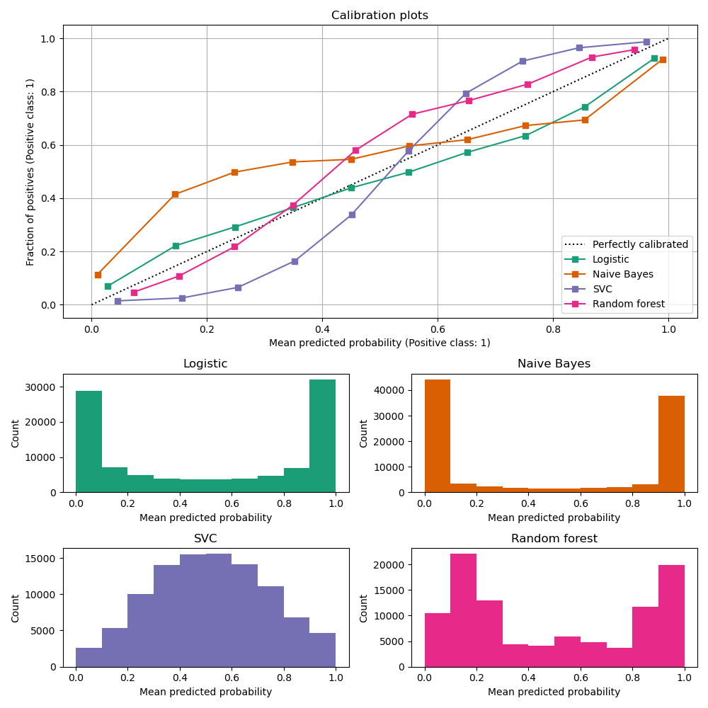
-
Logistic regression returns well calibrated predictions by default as it directly optimizes Log loss. In contrast, the other methods return biased probabilities; with different biases per method:
-
Naive Bayes tends to push probabilities to 0 or 1 (note the counts in the histograms). This is mainly because it makes the assumption that features are conditionally independent given the class, which is not the case in this dataset which contains 2 redundant features.
-
Random Forest Classifier shows the opposite behavior: the histograms show peaks at approximately 0.2 and 0.9 probability, while probabilities close to 0 or 1 are very rare. An explanation for this is given by Niculescu-Mizil and Caruana 1: “Methods such as bagging and random forests that average predictions from a base set of models can have difficulty making predictions near 0 and 1 because variance in the underlying base models will bias predictions that should be near zero or one away from these values. Because predictions are restricted to the interval [0,1], errors caused by variance tend to be one-sided near zero and one. For example, if a model should predict p = 0 for a case, the only way bagging can achieve this is if all bagged trees predict zero. If we add noise to the trees that bagging is averaging over, this noise will cause some trees to predict values larger than 0 for this case, thus moving the average prediction of the bagged ensemble away from 0. We observe this effect most strongly with random forests because the base-level trees trained with random forests have relatively high variance due to feature subsetting.” As a result, the calibration curve also referred to as the reliability diagram (Wilks 1995) shows a characteristic sigmoid shape, indicating that the classifier could trust its “intuition” more and return probabilities closer to 0 or 1 typically.
-
Linear Support Vector Classification (
LinearSVC) shows an even more sigmoid curve thanRandomForestClassifier, which is typical for maximum-margin methods (compare Niculescu-Mizil and Caruana), which focus on difficult to classify samples that are close to the decision boundary (the support vectors).
Calibrating a classifier
- Calibrating a classifier consists of fitting a regressor (called a calibrator) that maps the output of the classifier (as given by
decision_functionorpredict_proba) to a calibrated probability in[0, 1]. Denoting the output of the classifier for a given sample by \(f_{i}\), the calibrator tries to predict \(p\left(y_{i}=1 \mid f_{i}\right)\). - The samples that are used to fit the calibrator should not be the same samples used to fit the classifier, as this would introduce bias. This is because performance of the classifier on its training data would be better than for novel data. Using the classifier output of training data to fit the calibrator would thus result in a biased calibrator that maps to probabilities closer to 0 and 1 than it should.
Usage
- The CalibratedClassifierCV class from scikit-Learn is used to calibrate a classifier.
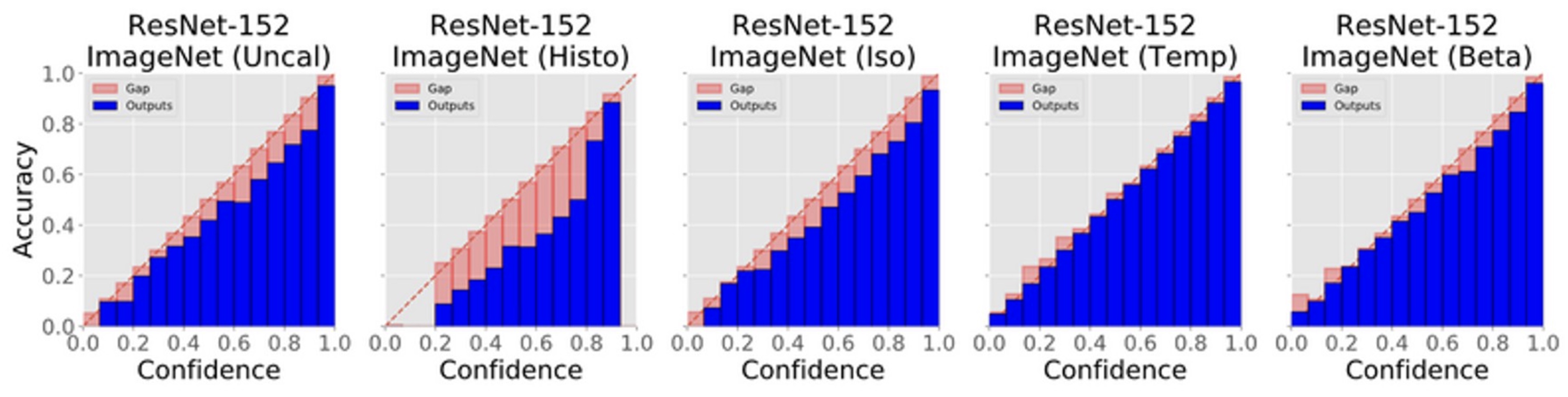
Effect of various calibration methods
- The figure below shows the gap between confidence and accuracy of the popular Resnet-152 on ImageNet, before and after various calibrations. From the diagram below, it is apparent that you can see temperature scaling closes the gap best.
Common Calibration Methods
- The following calibration methods are commonly used:
- Histogram binning - based on paper “Obtaining calibrated probability estimates from decision trees and naive bayesian classifiers”
- Isotonic regression - based on paper “Transforming classifier scores into accurate multiclass probability estimates”
- Temperature Scaling - based on paper “On Calibration of Modern Neural Networks”
- Beta Calibration - based on paper “Beta calibration: a well-founded and easily implemented improvement on logistic calibration for binary classifiers”
Brier score: Calibration metric
- Calibration can be represented using the Brier score which is the MSE between the actual and the estimated probabilities.
Implementation
- This Github repository contains all scripts needed to train neural networks (ResNet, DenseNet, DAN, etc.) and to calibrate the probabilities. These networks are trained on 4 different datasets and the model weights and output logits are available for use in this repository.
References
Citation
If you found our work useful, please cite it as:
@article{Chadha2020DistilledProbabilityCalibration,
  title   = {Probability Calibration},
  author  = {Chadha, Aman},
  journal = {Distilled AI},
  year    = {2020},
  note    = {\url{https://aman.ai}}
}