Aman's AI Journal • Primers • Physical AI

Overview
Foundations of Embodied Intelligence
Learning to Act
Vision-Language-Action Models
Isaac GR00T and Humanoid Foundation Models
Autonomous Driving as Physical AI
World Models for Physical AI
The Physical AI Data Engine
Training and Post-Training
Autonomy and Agentic Physical AI
Simulation, Sim-to-Real, and Digital Twins
Evaluation
Safety and Reliability for Physical AI
Engineering a Physical AI System
Open Problems and Research Directions
References
Citation

Overview

Physical AI combines perception, decision-making, and control in systems whose actions change their environment. The following sections establish its scope, operating loop, principal model families, and application domains.

Definition

What is Physical AI?

What is Physical AI? centers on a feedback process in which observations condition actions and those actions determine the next observations, making dynamics, latency, and recovery inseparable from model quality.
Physical AI refers to artificial intelligence systems that perceive, reason about, and act within the physical world. Unlike models whose outputs terminate in digital artifacts such as text, images, or software, a Physical AI system closes the loop between computation and physical consequences:
\[\text{Perceive} \rightarrow \text{Understand} \rightarrow \text{Reason} \rightarrow \text{Plan} \rightarrow \text{Act} \rightarrow \text{Observe consequences}\]
The defining feature is therefore not simply that AI is installed inside a physical machine. The system must continually map multimodal observations of the world into actions, observe how those actions alter the world, and adapt subsequent decisions accordingly.
A useful abstraction is a policy:
\[\pi_\theta(a_t \mid o_{\leq t}, g)\]
- where $o_{\leq t}$ represents the observation history, $g$ represents a goal or instruction, and $a_t$ represents an action executed in the physical environment. The action changes the state of that environment, producing the next observation:
  \[s_{t+1} \sim P(s_{t+1}\mid s_t,a_t)\] \[o_{t+1} \sim O(o_{t+1}\mid s_{t+1})\]
Physical AI therefore sits at the intersection of machine learning, robotics, computer vision, reinforcement learning, planning, control, simulation, and increasingly multimodal foundation models. In practice, the representation must preserve the task-relevant geometry, state, and uncertainty needed by downstream reasoning and control rather than only semantic appearance.
NVIDIA Cosmos World Foundation Model Platform for Physical AI by NVIDIA et al. (2025) frames the problem around two complementary learned representations: a policy model representing the intelligent agent and a world model representing the environment in which the agent operates.

From Digital Intelligence to Physical Intelligence

From Digital Intelligence to Physical Intelligence centers on a feedback process in which observations condition actions and those actions determine the next observations, making dynamics, latency, and recovery inseparable from model quality.
From Digital Intelligence to Physical Intelligence should be evaluated through the behavior it produces after integration, because component-level metrics can miss timing, state-distribution, and control-interface failures that only appear in closed-loop execution.
Large language models operate primarily over discrete tokens:
\[x_1,x_2,\ldots,x_T\]
A language model learns $p(x_t\mid x_{<t})$ and generates another token. The cost of an incorrect prediction is generally informational rather than immediately physical.
Physical intelligence introduces a fundamentally different loop. An autonomous system may observe camera images, depth, LiDAR, proprioception, force measurements, navigation information, or other sensors:
\[o_t = \{ I_t^{1:N}, d_t, q_t, \dot q_t, f_t, \ldots \}\]
- and must convert them into physically executable outputs such as joint positions, torques, end-effector poses, gripper commands, steering, acceleration, braking, or trajectories.
The system therefore learns a mapping closer to
\[(o_{\leq t},g) \xrightarrow{\pi_\theta} a_{t:t+H}\]
- where $a_{t:t+H}$ can be an action chunk or trajectory spanning a future horizon $H$.
The important distinction is that the prediction becomes an intervention. An erroneous text token can be regenerated; an erroneous steering trajectory, grasp, or humanoid motion can cause an irreversible physical transition.
This makes several problems that are secondary in conventional generative AI central to Physical AI: latency, dynamics, geometry, uncertainty, collision avoidance, embodiment constraints, temporal consistency, recovery, and safety. Its usefulness therefore depends less on visual plausibility alone than on whether predicted state changes preserve the consequences that would alter a downstream decision.

The Physical Intelligence Loop

This section develops the perception-reasoning-action loop in the context of the broader Physical AI system. It connects the underlying concepts to the implementation details discussed below.

The Perception-Reasoning-Action Loop

The Perception-Reasoning-Action Loop interleaves interpretation, action, and new environmental evidence so reasoning can be revised when the world does not respond as predicted.
The Perception-Reasoning-Action Loop should connect semantic intent to the current physical state and available actions, with execution feedback used to verify that the chosen interpretation actually produced the intended effect.
A useful conceptual decomposition consists of five interacting layers. In practice, the representation must preserve the task-relevant geometry, state, and uncertainty needed by downstream reasoning and control rather than only semantic appearance.

Perception

The system converts raw sensor measurements into representations of its surroundings. Modern Physical AI increasingly uses pretrained vision or vision-language representations rather than task-specific perception alone.
For a robot receiving images $I_t$ and language instruction $l$, a multimodal encoder may produce
\[z_t = f_{\mathrm{VLM}}(I_t,l)\]
This representation can encode objects, spatial relationships, semantic concepts, task intent, and eventually information relevant to action generation. In practice, the representation must preserve the task-relevant geometry, state, and uncertainty needed by downstream reasoning and control rather than only semantic appearance.
PaLM-E: An Embodied Multimodal Language Model by Driess et al. (2023) was an important step toward directly incorporating continuous sensor modalities into a language-model-centered architecture, establishing a path from multimodal foundation models toward embodied reasoning.

Reasoning

Reasoning determines what the observations mean relative to the agent’s goal. For example, a household robot instructed to “put away the groceries” must infer objects, destinations, ordering constraints, graspability, and possibly intermediate actions. Reasoning is particularly valuable when instructions underspecify the required physical behavior. Do As I Can, Not As I Say: Grounding Language in Robotic Affordances by Ahn et al. (2022) introduced SayCan, which combines language-model estimates of useful actions with learned affordance estimates of which actions are feasible in the current environment.
One simplified interpretation is
\[\pi(a\mid s,l) \propto p_{\mathrm{LLM}}(a\mid l) \, p_{\mathrm{affordance}}(\text{success}\mid s,a)\]
The first term asks whether an action makes semantic sense; the second asks whether the physical world currently permits it. For embodied use, that semantic interpretation must remain tied to the current scene, the robot state, and the actions that are actually feasible for the embodiment.
This distinction remains central to Physical AI. A model may know that a cup belongs in a cupboard without knowing whether the robot can currently reach the cupboard.

Planning

Planning converts goals into future actions or intermediate subgoals. A useful plan therefore has to connect high-level intent to reachable intermediate states and leave room to replan when execution produces an unexpected observation.
Classical robotics often makes this separation explicit:
\[\text{Perception} \rightarrow \text{World Model} \rightarrow \text{Planner} \rightarrow \text{Controller}\]
Foundation-model-based systems increasingly blur these boundaries. A VLA may predict low-level actions directly, while another architecture may use a large multimodal model for semantic planning and a specialized action model for continuous control. This latter separation is especially important in modern humanoid foundation models. GR00T N1: An Open Foundation Model for Generalist Humanoid Robots by NVIDIA et al. (2025) uses a dual-system architecture in which a vision-language component interprets observations and instructions while a Diffusion Transformer generates continuous robot actions.
The architecture illustrates an emerging pattern:
\[\text{slow semantic reasoning} + \text{fast continuous control}\]
This resembles the division between high-level deliberation and low-level motor behavior required by biological agents. In practice, the representation must preserve the task-relevant geometry, state, and uncertainty needed by downstream reasoning and control rather than only semantic appearance.

Action

The final output must be translated into commands supported by the embodiment. This is the point where learned predictions meet coordinate frames, control rates, actuator limits, and the closed-loop dynamics of the physical system.
For a manipulator, an action might be
\[a_t = [ \Delta x, \Delta y, \Delta z, \Delta \phi, \Delta \theta, \Delta \psi, g ]\]
- where the first six terms describe an end-effector pose displacement and $g$ controls the gripper.
Humanoids can require much higher-dimensional action vectors involving two arms, hands, torso, legs, and locomotion. Autonomous vehicles instead predict steering and acceleration commands or future trajectories.
This diversity creates the embodiment problem: two agents may understand the same instruction but require completely different motor representations to execute it. For embodied use, that semantic interpretation must remain tied to the current scene, the robot state, and the actions that are actually feasible for the embodiment.

Feedback

Physical action generates new observations, making control inherently closed-loop:
\[o_t \rightarrow a_t \rightarrow o_{t+1} \rightarrow a_{t+1} \rightarrow \cdots\]
This distinction between open-loop prediction and closed-loop interaction becomes especially important in autonomous driving. This is the point where learned predictions meet coordinate frames, control rates, actuator limits, and the closed-loop dynamics of the physical system.
A trajectory that looks plausible when evaluated against a recorded driving log may behave very differently when its own actions alter subsequent states. NVIDIA’s Alpamayo platform therefore couples reasoning VLAs with AlpaSim for closed-loop simulation and AlpaGym for reinforcement learning against the consequences of driving decisions.

Physical AI, Embodied AI, and Autonomy

Physical AI, Embodied AI, and Autonomy centers on a feedback process in which observations condition actions and those actions determine the next observations, making dynamics, latency, and recovery inseparable from model quality.
Physical AI, Embodied AI, and Autonomy benefits from explicit progress and completion signals so the agent can tell whether a subgoal actually changed the world as intended, rather than assuming that a plausible sequence of actions will compose successfully.
These terms overlap but describe somewhat different concepts. Embodied AI focuses on intelligence situated in an agent that interacts with an environment through perception and action. Embodiment matters because the agent’s capabilities, observations, and learning signals are constrained by its body. Physical AI is somewhat broader in current usage. It encompasses embodied robots but also autonomous vehicles, industrial systems, drones, and other AI systems whose decisions interact directly with physical dynamics.
Autonomy describes the degree to which such a system can pursue objectives without continuous human control. This is the point where learned predictions meet coordinate frames, control rates, actuator limits, and the closed-loop dynamics of the physical system.
A useful hierarchy is:
\[\text{Physical AI} \supset \{ \text{Robotics}, \text{Autonomous Driving}, \text{Industrial Autonomy}, \ldots \}\]
Embodied intelligence provides many of the learning principles underlying these systems, while autonomy describes how independently the resulting system operates. Reliable autonomy therefore requires explicit progress state, completion conditions, and recovery behavior rather than assuming that a plausible next action will compose into a successful long-horizon trajectory.
A robot executing a preprogrammed trajectory is physical automation but exhibits little learned autonomy. A robot that understands a natural-language goal, recognizes unfamiliar objects, decomposes the task, manipulates them, detects failures, and replans represents a substantially richer form of Physical AI.

Core Capabilities

This section develops from robotics models to robot foundation models in the context of the broader Physical AI system. It connects the underlying concepts to the implementation details discussed below.

From Robotics Models to Robot Foundation Models

From Robotics Models to Robot Foundation Models defines which parts of perception, reasoning, and control share a pretrained representation and which remain specialized, a boundary that governs transfer, latency, interpretability, and embodiment adaptation.
From Robotics Models to Robot Foundation Models should distinguish broadly reusable semantic and perceptual representations from robot-specific calibration in kinematics, dynamics, sensing, action ranges, and recovery behavior.
Traditional learned robot policies were typically specialized:
\[\pi_{\theta}^{(\text{task},\text{robot},\text{environment})}\]
Changing the robot, camera configuration, task, or environment could require training another policy. This is the point where learned predictions meet coordinate frames, control rates, actuator limits, and the closed-loop dynamics of the physical system.
The foundation-model paradigm instead seeks a shared policy:
\[\pi_\theta ( a \mid o, l, e )\]
- where $e$ describes or implicitly identifies the embodiment.
The objective is to transfer knowledge across
\[\text{tasks} \times \text{environments} \times \text{objects} \times \text{embodiments}\]
Open X-Embodiment: Robotic Learning Datasets and RT-X Models by Open X-Embodiment Collaboration et al. (2023) demonstrated this direction by standardizing data from 22 robot embodiments and showing positive transfer from cross-robot training. Octo: An Open-Source Generalist Robot Policy by Octo Model Team et al. (2024) subsequently trained a transformer policy on approximately 800,000 Open X-Embodiment trajectories and designed the model so that new observations and action spaces could be incorporated during fine-tuning.
The shift mirrors the evolution of NLP:
\[\text{task-specific model} \rightarrow \text{pretrained foundation model} \rightarrow \text{adaptation}\]
In robotics:
\[\text{task-specific policy} \rightarrow \text{generalist robot foundation model} \rightarrow \text{embodiment/task post-training}\]

Vision-Language-Action Models

Vision-Language-Action models extend multimodal understanding into control by conditioning action prediction on visual observations, language instructions, and robot state; their central design problem is how to convert broad semantic features into action representations that remain executable under the robot’s kinematics and control loop.
Vision-Language-Action Models should connect semantic intent to the current physical state and available actions, with execution feedback used to verify that the chosen interpretation actually produced the intended effect.
One of the most consequential architectural developments in Physical AI is the Vision-Language-Action model, or VLA. A VLA extends the familiar vision-language mapping $(I,l) \rightarrow \text{text}$ into $(I,l,s)\rightarrow a$. The model therefore connects semantic representations learned from large-scale image-text corpora to physically executable behavior.
RT-2: Vision-Language-Action Models Transfer Web Knowledge to Robotic Control by Brohan et al. (2023) established the VLA formulation by representing robot actions as tokens and co-fine-tuning vision-language models on web-scale vision-language tasks and robotic trajectories. This allowed semantic knowledge learned from the web to influence robot behavior. OpenVLA: An Open-Source Vision-Language-Action Model by Kim et al. (2024) provided an open 7B-parameter implementation trained on 970,000 real-world robot demonstrations, combining DINOv2 and SigLIP visual features with a Llama-family language backbone.
Robot control no longer has to begin from a blank policy network. A Physical AI system can inherit semantic knowledge about objects, concepts, relationships, and instructions from large-scale multimodal pretraining and then ground this knowledge through robot demonstrations.

Continuous Generative Action Models

Continuous Generative Action Models models a conditional distribution over continuous action sequences, making multimodal demonstrations and several valid motion strategies representable without averaging them into an invalid mean action.
Continuous Generative Action Models should be evaluated through the behavior it produces after integration, because component-level metrics can miss timing, state-distribution, and control-interface failures that only appear in closed-loop execution.
Physical actions differ fundamentally from language tokens. Robot motion is typically continuous, temporally correlated, and multimodal.
Suppose two valid demonstrations move around opposite sides of an obstacle. A regression policy minimizing:
\[\mathcal{L}_{\mathrm{MSE}} = \mathbb{E} \left[ \left\| a-\pi_\theta(o) \right\|_2^2 \right]\]
- can average the two behaviors and generate an action corresponding to neither valid trajectory.
Generative action models address this by learning distributions over actions. Diffusion Policy: Visuomotor Policy Learning via Action Diffusion by Chi et al. (2023) formulates robot control as conditional denoising diffusion, allowing policies to represent multimodal high-dimensional action distributions and generate action sequences under receding-horizon control. This idea has become increasingly important in robot foundation models. GR00T, for example, combines semantic VLM representations with a Diffusion Transformer action model rather than requiring the language model itself to generate every continuous motor command.
The architecture can be abstracted as:
\[z = f_{\mathrm{VLM}}(I,l)\]
- followed by
  \[a_{t:t+H} = f_{\mathrm{action}}(z,s_t)\]
This separation allows large-scale semantic representations and specialized continuous control architectures to complement each other. For embodied use, that semantic interpretation must remain tied to the current scene, the robot state, and the actions that are actually feasible for the embodiment.

Models and Learning

This section develops physical ai as a data problem in the context of the broader Physical AI system. It connects the underlying concepts to the implementation details discussed below.

Physical AI as a Data Problem

Physical AI as a Data Problem is governed by the distribution of physical experience available for learning: useful scale comes from covering tasks, embodiments, recovery states, and action consequences rather than simply accumulating more frames.
Physical AI as a Data Problem should be assessed by the new behavioral coverage it contributes, especially rare states, recovery situations, and observation-action combinations that are missing from the current training distribution.
The largest obstacle to scaling Physical AI is not simply model architecture. It is data. Internet-scale language and images are comparatively inexpensive. High-quality physical interaction trajectories require robots, environments, operators, sensors, calibration, and time.
A robot demonstration can be represented as
\[\tau = (o_0,a_0,o_1,a_1,\ldots,o_T)\]
Large robot foundation models require diverse distributions over such trajectories:
\[\mathcal{D} = \bigcup_{i=1}^{N} \mathcal{D}_i^{\text{embodiment}} \cup \mathcal{D}^{\text{simulation}} \cup \mathcal{D}^{\text{human}} \cup \mathcal{D}^{\text{synthetic}}\]
This motivates a Physical AI data flywheel:
\[\text{Real Data} \rightarrow \text{Model} \rightarrow \text{Simulation/Synthetic Data} \rightarrow \text{Training} \rightarrow \text{Deployment} \rightarrow \text{New Real Data}\]
GR00T N1 explicitly mixes real robot trajectories, human videos, and synthetic data, while later NVIDIA GR00T workflows use simulation and generative world models to expand the training distribution. Its usefulness therefore depends less on visual plausibility alone than on whether predicted state changes preserve the consequences that would alter a downstream decision.
Open X-Embodiment attacks the same bottleneck from another direction by pooling heterogeneous robot datasets, allowing experience from one embodiment to improve another. What matters is not only the number of examples but also their coverage of tasks, embodiments, recovery states, and observation-action alignments that the deployed policy will encounter.

World Models and Simulation

World Models and Simulation models how physical state evolves under actions, enabling counterfactual prediction, planning, synthetic experience, and closed-loop evaluation before every decision is attempted in the real world.
World Models and Simulation should vary or calibrate the physical and sensing factors that materially affect the deployed policy, with success measured by transfer to held-out real behavior rather than by simulator performance alone.
A policy answers:
\[\text{What should I do?}\]
A world model addresses:
\[\text{What will happen if I do it?}\]
Formally, a learned dynamics model approximates
\[p_\phi(s_{t+1}\mid s_t,a_t)\]
Given candidate future actions,
\[a_t,a_{t+1},\ldots,a_{t+H}\]
- the agent can predict possible futures before committing to them physically.
Mastering Diverse Domains through World Models by Hafner et al. (2023) develops DreamerV3, which learns environmental dynamics and improves its policy using imagined trajectories, illustrating the broader model-based principle that agents can learn from predicted experience rather than exclusively from physical interaction. Cosmos World Foundation Model Platform for Physical AI by NVIDIA et al. (2025) scales this idea toward general-purpose world foundation models that can be post-trained for robotics and autonomous-system applications.
This leads to an increasingly important architecture for Physical AI:
\[\boxed{ \text{Policy Foundation Model} + \text{World Foundation Model} + \text{Physics Simulator} }\]
The policy proposes behavior, the world model predicts plausible outcomes, and simulation provides an environment in which those behaviors can be trained and evaluated without incurring the cost and risk of every experiment in the real world. This is the point where learned predictions meet coordinate frames, control rates, actuator limits, and the closed-loop dynamics of the physical system.

Systems and Applications

This section develops physical ai across robots and autonomous vehicles in the context of the broader Physical AI system. It connects the underlying concepts to the implementation details discussed below.

Physical AI Across Robots and Autonomous Vehicles

Physical AI Across Robots and Autonomous Vehicles makes closed-loop effects especially visible because steering and braking alter the future traffic scene, so a trajectory must be evaluated through the states it causes rather than only against a recorded log.
Physical AI Across Robots and Autonomous Vehicles must be evaluated interactively because ego actions change the future traffic scene and can provoke different responses from other agents; fixed-log replay cannot capture those feedback effects.
Robotics and autonomous driving appear different at the actuator level but increasingly share the same learning abstractions. This is the point where learned predictions meet coordinate frames, control rates, actuator limits, and the closed-loop dynamics of the physical system.
For manipulation:
\[(\text{camera},\text{language},\text{proprioception}) \rightarrow \text{arm/hand trajectory}\]
For autonomous driving:
\[(\text{multi-camera video},\text{route},\text{vehicle state}) \rightarrow \text{vehicle trajectory}\]
NVIDIA’s Alpamayo applies the VLA paradigm to autonomous vehicles, processing multi-camera observations and driving context to produce trajectories together with explicit Chain-of-Causation reasoning traces. As of September 2026, the family extends to Alpamayo 2 Super, a 34B reasoning VLA accompanied by AlpaGym for closed-loop RL and generative simulation infrastructure for long-tail driving scenarios.
The architectural convergence is significant. Humanoid robotics and autonomous driving increasingly share the same broad recipe:
\[\text{multimodal perception} + \text{foundation-model reasoning} + \text{continuous action generation} + \\ \text{world models/simulation} + \text{closed-loop learning}\]
What differs is the embodiment, dynamics, action space, safety envelope, and deployment stack. This is the point where learned predictions meet coordinate frames, control rates, actuator limits, and the closed-loop dynamics of the physical system.

Toward Generalist Physical Agents

Toward Generalist Physical Agents should be analyzed along separate axes such as task, object, scene, language, dynamics, and embodiment because success on one axis does not imply broad physical generalization.
Toward Generalist Physical Agents should distinguish broadly reusable semantic and perceptual representations from robot-specific calibration in kinematics, dynamics, sensing, action ranges, and recovery behavior.
The long-term objective is not simply a robot capable of executing a larger catalog of memorized skills. It is an agent that can transfer knowledge to new physical situations.
$\pi_{0.5}$: a Vision-Language-Action Model with Open-World Generalization by Physical Intelligence et al. (2025) combines robot data, web data, high-level semantic prediction, and heterogeneous multimodal examples to target this problem, demonstrating long-horizon manipulation in previously unseen homes.
General physical intelligence therefore requires generalization along several axes:
\[G = G_{\text{task}} \times G_{\text{object}} \times G_{\text{scene}} \times G_{\text{embodiment}} \times G_{\text{dynamics}} \times G_{\text{instruction}}\]
A system that generalizes only to a differently colored object has solved a much narrower problem than one that transfers a learned concept between robot embodiments, environments, and task compositions. Transfer is therefore easiest for semantic and perceptual structure, while action normalization, kinematics, reachable states, and safety limits still require embodiment-aware handling.
This is why Physical AI increasingly looks less like conventional robotics with a larger neural network and more like a complete foundation-model stack for interacting with reality:
\[\boxed{ \begin{array}{c} \text{Multimodal Foundation Models}\\ \downarrow\\ \text{World Models + Physical Reasoning}\\ \downarrow\\ \text{Planning + VLA Policies}\\ \downarrow\\ \text{Continuous Control}\\ \downarrow\\ \text{Physical Environment}\\ \downarrow\\ \text{Feedback + Data}\\ \circlearrowleft \end{array} }\]
The remainder of the primer will unpack each layer, beginning with the foundations of embodied intelligence and the progression from classical perception-planning-control pipelines to modern multimodal embodied foundation models. In practice, the representation must preserve the task-relevant geometry, state, and uncertainty needed by downstream reasoning and control rather than only semantic appearance.

Foundations of Embodied Intelligence

Embodied intelligence depends on the relationship between sensing, physical constraints, learning, and interaction. These foundations explain how robot policies connect abstract goals to actions in changing environments.

Embodiment and Formal Foundations

This section develops embodiment as a computational constraint in the context of the broader Physical AI system. It connects the underlying concepts to the implementation details discussed below.

Embodiment as a Computational Constraint

Embodiment as a Computational Constraint distinguishes reusable semantic and perceptual structure from the robot-specific kinematics, dynamics, sensing, and action conventions required for successful execution.
Embodiment as a Computational Constraint requires enforcement outside the learned policy for constraints that must hold even when the model is uncertain, out of distribution, or wrong.
Embodied intelligence studies agents whose cognition is coupled to a body and an environment. The central idea is that intelligence in the physical world cannot be reduced to mapping abstract inputs to abstract outputs: what an agent can observe, infer, and accomplish depends on its sensors, actuators, morphology, dynamics, and interaction history. A Survey on Robotics with Foundation Models: toward Embodied AI by Xu et al. (2024) characterizes embodied AI as integrating perception, learning, reasoning, decision-making, control, and generalization so that agents can perform tasks in open, dynamic environments.
Consider two agents observing the same cup. A language model may represent the cup semantically, while a robot must additionally reason about whether the cup is reachable, how it should be grasped, whether it is full, how much force is appropriate, and how its own kinematics constrain the motion.
Thus, an embodied agent operates under a coupling
\[\text{Intelligence} = f( \text{Model}, \text{Body}, \text{Environment}, \text{Interaction} )\]
The body is not merely the output device for an otherwise independent intelligence. It determines the agent’s action space, observation space, reachable states, and physical constraints.
For example, a manipulator might expose an action
\[a_t = [ \Delta x_t, \Delta y_t, \Delta z_t, \Delta r_t, \Delta p_t, \Delta y_t^{\mathrm{rot}}, g_t ]\]
- while a humanoid may instead expose dozens of joint targets:
  \[a_t = [ q_{1,t}^{*}, q_{2,t}^{*}, \ldots, q_{n,t}^{*} ]\]
A mobile robot may operate through linear and angular velocity,
\[a_t = [v_t,\omega_t]\]
- and an autonomous vehicle may execute steering, acceleration, and braking commands.
The same semantic objective, move the object from the table to the shelf, induces different policies for different embodiments.
This gives rise to the embodiment gap: knowledge may transfer between robots even when executable behavior does not. The Embodiment Gap in Robot Foundation Models by Domae et al. (2026) formalizes this distinction by separating reusable semantic, perceptual, data, and representation-level knowledge from the adaptation still required to execute successfully on a new robot.

The Agent-Environment Loop

The Agent-Environment Loop evaluates behavior through the feedback loop created when each action changes the next state and observation, exposing compounding errors that static prediction metrics can hide.
The Agent-Environment Loop benefits from explicit progress and completion signals so the agent can tell whether a subgoal actually changed the world as intended, rather than assuming that a plausible sequence of actions will compose successfully.
The canonical abstraction for embodied intelligence is an agent interacting sequentially with an environment. This is the point where learned predictions meet coordinate frames, control rates, actuator limits, and the closed-loop dynamics of the physical system.
At time $t$:
1. the environment occupies state $s_t$;
2. the agent receives observation $o_t$;
3. the policy selects action $a_t$;
4. the environment transitions to $s_{t+1}$;
5. the agent receives the next observation.
Formally,
\[o_t \sim O(o_t\mid s_t)\] \[a_t \sim \pi_\theta(a_t\mid o_{\leq t},g)\] \[s_{t+1}\sim P(s_{t+1}\mid s_t,a_t)\]
The resulting trajectory is
\[\tau = (s_0,o_0,a_0,s_1,o_1,a_1,\ldots,s_T)\]
This sequential structure is fundamental. Physical intelligence is not a collection of independent predictions because an action changes the distribution of observations the agent will subsequently receive. For example, moving a camera changes the visual observation. Moving a robot arm may occlude an object. Picking up an object changes its pose. Steering a vehicle changes which future traffic configurations are encountered.
The policy therefore influences its own future input distribution:
\[\pi_\theta \rightarrow P(s_{t+1}) \rightarrow P(o_{t+1}) \rightarrow \pi_\theta\]
This feedback loop is one reason physical agents are substantially harder to evaluate than static vision or language models. In practice, the representation must preserve the task-relevant geometry, state, and uncertainty needed by downstream reasoning and control rather than only semantic appearance.

Embodied Intelligence as a POMDP

Embodied Intelligence as a POMDP formalizes the fact that the agent rarely observes the complete physical state directly. History, internal state, and uncertainty estimates therefore matter because two visually similar observations can require different actions when their hidden histories or task phases differ.
Embodied Intelligence as a POMDP should be evaluated through the behavior it produces after integration, because component-level metrics can miss timing, state-distribution, and control-interface failures that only appear in closed-loop execution.
Most real-world embodied tasks are naturally modeled as partially observable Markov decision processes, or POMDPs. The key systems implication is that model quality must ultimately be judged through executable behavior under the sensing, dynamics, and timing constraints of the physical platform.
A POMDP can be written as
\[\mathcal{M} = (\mathcal{S}, \mathcal{A}, \mathcal{O}, P, O, R, \gamma)\]
- where:
$\mathcal{S}$ is the latent physical state space; $\mathcal{A}$ is the action space; $\mathcal{O}$ is the observation space; $P(s_{t+1}\mid s_t,a_t)$ is the transition model; In practice, the representation must preserve the task-relevant geometry, state, and uncertainty needed by downstream reasoning and control rather than only semantic appearance.
$O(o_t\mid s_t)$ is the observation model; $R(s_t,a_t)$ is the reward; $\gamma$ is the discount factor. The agent generally cannot observe $s_t$ directly.
A camera cannot see behind an occluding object. A robot may not know an object’s mass until interacting with it. A vehicle approaching an intersection cannot directly observe another driver’s intention.
The policy must therefore condition on history,
\[\pi_\theta(a_t\mid o_{\leq t},a_{<t},g)\]
- or maintain an internal state:
  \[h_t = f_\theta( h_{t-1}, o_t, a_{t-1} )\]
The policy then becomes:
\[a_t\sim\pi_\theta(a_t\mid h_t,g)\]
Transformers are particularly attractive here because the context window can implicitly function as a finite interaction memory:
\[h_t = \operatorname{Transformer} ( o_{t-k:t}, a_{t-k:t-1}, g )\]
This connection helps explain why architectures developed for sequence modeling transferred naturally into robotics. The stronger test is whether the learned representation and policy continue to work when several factors shift together rather than when only one superficial attribute changes.

Perception Is Not Merely Object Recognition

Perception Is Not Merely Object Recognition asks perception to retain the geometry, state, and uncertainty that matter for action, not merely to assign semantic labels to the current scene.
Perception Is Not Merely Object Recognition should be evaluated through the behavior it produces after integration, because component-level metrics can miss timing, state-distribution, and control-interface failures that only appear in closed-loop execution.
Classical computer vision often decomposes perception into tasks such as detection, segmentation, pose estimation, depth estimation, and tracking. In practice, the representation must preserve the task-relevant geometry, state, and uncertainty needed by downstream reasoning and control rather than only semantic appearance.
Embodied perception asks a more operational question:
\[\text{What information is required to act successfully?}\]
Suppose a robot must pick up a mug. Recognizing the category “mug” is insufficient. The policy may require:
\[\{ \text{location}, \text{orientation}, \text{handle pose}, \text{free space}, \text{reachability}, \text{grasp points} \}\]
This distinction motivates representations optimized for action rather than exclusively for semantic recognition. In practice, the representation must preserve the task-relevant geometry, state, and uncertainty needed by downstream reasoning and control rather than only semantic appearance.
CLIPort: What and Where Pathways for Robotic Manipulation by Shridhar et al. (2021) combines CLIP-derived semantic representations for determining “what” should be manipulated with Transporter-style spatial representations for determining “where” manipulation should occur, demonstrating how semantic and geometric information can complement each other in language-conditioned manipulation.
A useful abstraction is therefore:
\[z_t = f_{\mathrm{perception}}(o_t)\]
- where $z_t$ should preserve information relevant to the downstream policy rather than reconstruct every property of the environment.

Learning Visual Representations from Human Activity

Learning Visual Representations from Human Activity uses human video to learn object state, contact, and temporal structure at scale, while robot-specific training later grounds those visual regularities into executable actions.
Learning Visual Representations from Human Activity should be evaluated through the behavior it produces after integration, because component-level metrics can miss timing, state-distribution, and control-interface failures that only appear in closed-loop execution.
Robot datasets are expensive, but humans generate enormous quantities of video showing interactions with the physical world. This motivates learning representations from human video and transferring them to robots.
R3M: A Universal Visual Representation for Robot Manipulation by Nair et al. (2022) pretrains visual representations on Ego4D human video using temporal contrastive learning, video-language alignment, and regularization, then uses the representation as a frozen perceptual backbone for robot policies.
Conceptually,
\[\text{Human Video} \xrightarrow{\text{pretraining}} f_\phi(I) \xrightarrow{\text{robot data}} \pi_\theta(a\mid f_\phi(I))\]
The important assumption is that visual regularities such as object state, contact, motion, and human-object interaction contain information that transfers across embodiments. In practice, the representation must preserve the task-relevant geometry, state, and uncertainty needed by downstream reasoning and control rather than only semantic appearance.
Human video does not directly specify robot actions:
\[a_t^{\mathrm{human}} \neq a_t^{\mathrm{robot}}\]
But it can teach representations of the physical world that make robot-specific learning more data efficient. In practice, the representation must preserve the task-relevant geometry, state, and uncertainty needed by downstream reasoning and control rather than only semantic appearance.
This distinction between transferable perceptual knowledge and embodiment-specific control will recur throughout Physical AI. In practice, the representation must preserve the task-relevant geometry, state, and uncertainty needed by downstream reasoning and control rather than only semantic appearance.

Perception and Language Grounding

This section develops grounding language in physical interaction in the context of the broader Physical AI system. It connects the underlying concepts to the implementation details discussed below.

Grounding Language in Physical Interaction

Grounding Language in Physical Interaction asks perception to retain the geometry, state, and uncertainty that matter for action, not merely to assign semantic labels to the current scene.
Grounding Language in Physical Interaction should connect semantic intent to the current physical state and available actions, with execution feedback used to verify that the chosen interpretation actually produced the intended effect.
Language models can encode substantial semantic knowledge but do not inherently know whether a particular physical action is executable in the current environment. For embodied use, that semantic interpretation must remain tied to the current scene, the robot state, and the actions that are actually feasible for the embodiment.
Consider the instruction: “Bring me the apple.” A language model can infer plausible subgoals:
\[\text{find apple} \rightarrow \text{approach apple} \rightarrow \text{pick apple} \rightarrow \text{return}\]
But successful execution additionally requires answering questions such as:
Is an apple visible? Is it reachable? Is the gripper already occupied? Can the robot navigate to it?
Is the proposed grasp physically feasible? Do As I Can, Not As I Say: Grounding Language in Robotic Affordances by Ahn et al. (2022) introduced SayCan to connect semantic reasoning from large language models with learned robotic affordances.
Let $l$ denote the instruction and $s$ the current physical state. A simplified decomposition is
\[\operatorname{score}(a) = p_{\mathrm{LLM}}(a\mid l) \, Q(s,a)\]
- where $p_{\mathrm{LLM}}(a\mid l)$ captures whether the action is useful for satisfying the instruction, while $Q(s,a)$ estimates whether the robot can successfully execute it.
The highest-scoring action is selected:
\[a^* = \arg\max_a p_{\mathrm{LLM}}(a\mid l)Q(s,a)\]
This separates two distinct questions: $\text{Should I do this?}$ and $\text{Can I do this?}$.
The distinction between semantic plausibility and physical feasibility remains one of the foundational ideas behind modern embodied agents. For embodied use, that semantic interpretation must remain tied to the current scene, the robot state, and the actions that are actually feasible for the embodiment.

Affordances

Affordances represents perception in terms of actions available to a particular embodiment, connecting object and scene understanding to what the robot can successfully do from the current state.
Affordances should be evaluated through the behavior it produces after integration, because component-level metrics can miss timing, state-distribution, and control-interface failures that only appear in closed-loop execution.
The concept underlying SayCan is broader than robotics foundation models. An affordance describes an action that an environment or object makes available to an agent.
A cup may afford $\{\text{grasp},\text{lift},\text{pour},\text{place}\}$, while a closed drawer may afford $\{\text{grasp handle}, \text{pull}\}$.
Critically, affordances depend on the agent. A shelf may be reachable for a humanoid but not for a short mobile manipulator. A heavy object may be liftable by one robot but not another.
Thus an affordance is more accurately modeled as
\[A(s,e,a)\]
- where $s$ describes the environment, $e$ describes the embodiment, and $a$ is a candidate action.
This makes affordances a natural bridge between semantic reasoning and physical control. For embodied use, that semantic interpretation must remain tied to the current scene, the robot state, and the actions that are actually feasible for the embodiment.

From Modular Robotics to Learned Policies

Explicit perception, state-estimation, planning, and control modules make intermediate assumptions testable, while learned policies trade some of that modularity for representations optimized jointly with the downstream task.
From Modular Robotics to Learned Policies should be evaluated through the behavior it produces after integration, because component-level metrics can miss timing, state-distribution, and control-interface failures that only appear in closed-loop execution.
Classical autonomous robots are frequently organized as explicit modules:
\[\boxed{ \text{Sensors} \rightarrow \text{Perception} \rightarrow \text{State Estimation} \rightarrow \text{Planning} \rightarrow \text{Control} \rightarrow \text{Actuators} }\]
Each component exposes a structured interface. The key systems implication is that model quality must ultimately be judged through executable behavior under the sensing, dynamics, and timing constraints of the physical platform.
For example:
\[I_t \xrightarrow{\text{detector}} \text{objects} \xrightarrow{\text{pose estimator}} \text{6D poses} \xrightarrow{\text{planner}} \text{trajectory} \xrightarrow{\text{controller}} \text{torques}\]
This architecture has substantial engineering advantages. Intermediate states are interpretable, components can be independently tested, and known physical constraints can be incorporated explicitly. However, every interface potentially discards information.
A learned policy instead attempts
\[\pi_\theta: (o_t,g)\rightarrow a_t\]
The extreme version is end-to-end control:
\[\text{pixels} \rightarrow \text{actions}\]
Modern Physical AI increasingly occupies a middle ground. Large learned representations replace many hand-engineered perception and reasoning components, while structured planners, controllers, safety systems, or specialized action heads remain useful.
The important architectural question is therefore no longer simply “modular or end-to-end.” It is:
\[\text{Which abstractions should be learned, and where should structure be retained?}\]

Imitation Learning as the Basic Robot-Learning Primitive

Imitation Learning as the Basic Robot-Learning Primitive learns directly from demonstrated observation-action pairs, but robust deployment depends on whether those demonstrations cover the states the policy will reach after its own inevitable small errors.
Imitation Learning as the Basic Robot-Learning Primitive should be evaluated through the behavior it produces after integration, because component-level metrics can miss timing, state-distribution, and control-interface failures that only appear in closed-loop execution.
Much modern embodied AI begins with demonstrations. What matters is not only the number of examples but also their coverage of tasks, embodiments, recovery states, and observation-action alignments that the deployed policy will encounter.
Given a dataset $\mathcal{D} = \{(o_t^{(i)},g^{(i)},a_t^{(i)})\}$ behavioral cloning trains the policy to reproduce demonstrated actions:
\[\mathcal{L}_{\mathrm{BC}}(\theta) = -\mathbb{E}_{(o,g,a)\sim\mathcal{D}} [ \log \pi_\theta(a\mid o,g) ]\]
For continuous deterministic actions, this may reduce to regression:
\[\mathcal{L}_{\mathrm{BC}} = \mathbb{E} \left[ \| a-\hat a_\theta \|_2^2 \right]\]
The attraction is straightforward: humans demonstrate successful behavior, and the robot learns the mapping from observations and instructions to actions. The difficulty is distribution shift.
During training:
\[o_t \sim p_{\mathrm{expert}}(o)\]
During deployment:
\[o_t \sim p_{\pi_\theta}(o)\]
A small prediction error may place the robot in a state absent from the demonstration dataset. Subsequent predictions then become less reliable, producing compounding error.
This is one reason temporal action modeling, large diverse datasets, intervention data, simulation, and reinforcement-learning post-training become important. For embodied use, that semantic interpretation must remain tied to the current scene, the robot state, and the actions that are actually feasible for the embodiment.

Scaling Demonstrations Enables Generalization

Scaling Demonstrations Enables Generalization learns directly from demonstrated observation-action pairs, but robust deployment depends on whether those demonstrations cover the states the policy will reach after its own inevitable small errors.
Scaling Demonstrations Enables Generalization should be assessed by the new behavioral coverage it contributes, especially rare states, recovery situations, and observation-action combinations that are missing from the current training distribution.
Early robot-learning systems often learned one task from one dataset. A major transition occurred when researchers began asking whether a sufficiently diverse demonstration distribution could produce general-purpose behavior.
BC-Z: Zero-Shot Task Generalization with Robotic Imitation Learning by Jang et al. (2022) scaled imitation learning beyond 100 manipulation tasks and conditioned policies using language or human-video task representations, demonstrating zero-shot execution on previously unseen manipulation tasks.
Instead of training $\pi_{\theta,k}(a\mid o)$ for each task $k$, the objective becomes a shared conditioned policy $\pi_\theta(a\mid o,g)$.
The task descriptor $g$ can take multiple forms:
\[g \in \{ \text{text}, \text{image}, \text{video}, \text{goal state}, \text{demonstration} \}\]
This transition is foundational because it converts task identity from something encoded in the model weights into something specified at inference time. What matters is not only the number of examples but also their coverage of tasks, embodiments, recovery states, and observation-action alignments that the deployed policy will encounter.

Robot Learning Fundamentals

This section develops multimodal prompting for robots in the context of the broader Physical AI system. It connects the underlying concepts to the implementation details discussed below.

Multimodal Prompting for Robots

Multimodal robot prompts turn task specification into a combination of language and visual references, allowing one policy to condition behavior on objects, demonstrations, and goals without defining a new controller for each task.
Multimodal Prompting for Robots should connect semantic intent to the current physical state and available actions, with execution feedback used to verify that the chosen interpretation actually produced the intended effect.
Human instructions are rarely restricted to text. A person can communicate a task by pointing, demonstrating, showing an image, or combining visual and linguistic cues. VIMA: General Robot Manipulation with Multimodal Prompts by Jiang et al. (2022) formalizes robot tasks as multimodal prompts interleaving visual and textual tokens, and trains a transformer to autoregressively produce motor actions across thousands of procedurally generated manipulation tasks.
A prompt might conceptually take the form $p = [\text{"put"},I_{\mathrm{object}},\text{"inside"},I_{\mathrm{container}}]$.
The policy becomes:
\[\pi_\theta(a_t\mid o_{\leq t},p)\]
This is a significant conceptual change. Rather than defining each robotic task through a separate reward function or policy, tasks become prompts to a shared embodied model.
The idea foreshadows modern VLA models, where natural-language instructions and visual observations jointly condition physical actions. In practice, the representation must preserve the task-relevant geometry, state, and uncertainty needed by downstream reasoning and control rather than only semantic appearance.

Action Chunking and Temporal Abstraction

Action Chunking and Temporal Abstraction predicts multiple temporally coupled actions together, improving motion coherence and amortizing inference while trading away some per-timestep responsiveness.
Action Chunking and Temporal Abstraction changes how the policy represents and executes motion, so the chosen temporal horizon and action parameterization must remain compatible with controller rate, embodiment limits, and opportunities for feedback correction.
A robot policy need not predict only one action at a time. This is the point where learned predictions meet coordinate frames, control rates, actuator limits, and the closed-loop dynamics of the physical system.
Instead of $\pi_\theta(o_t)\rightarrow a_t$, it can predict a chunk:
\[\pi_\theta(o_t) \rightarrow (a_t,a_{t+1},\ldots,a_{t+H})\]
Learning Fine-Grained Bimanual Manipulation with Low-Cost Hardware by Zhao et al. (2023) introduces Action Chunking with Transformers (ACT), using a conditional VAE and transformer architecture to generate sequences of actions for precise bimanual manipulation while mitigating compounding errors and temporal variability in human demonstrations.
ACT learns a distribution of action sequences,
\[p_\theta(a_{t:t+H}\mid o_t,z)\]
- where $z$ is a latent variable encoding variation in demonstrations.
A generic conditional VAE objective is
\[\mathcal{L}_{\mathrm{ACT}} = \mathbb{E}_{q_\phi(z\mid a,o)} [ -\log p_\theta(a\mid o,z) ] + \beta D_{\mathrm{KL}} \left( q_\phi(z\mid a,o) \| p(z) \right)\]
Action chunking provides temporal abstraction:
\[\text{observation} \rightarrow \underbrace{ [a_t,\ldots,a_{t+H}] }_{\text{coherent motion}}\]
- rather than requiring the policy to reconstruct the intended trajectory independently at every control step.
This concept later becomes important in VLAs and diffusion/flow-based action models. This is the point where learned predictions meet coordinate frames, control rates, actuator limits, and the closed-loop dynamics of the physical system.

Transformers Enter Robot Control

Transformers provide a natural way to model temporally ordered observations and actions, letting a robot policy condition each decision on task language and a finite history rather than on the latest frame alone.
Transformers Enter Robot Control must be analyzed as part of the timed execution path from observation to actuation, because stale state, wrong frames, or delayed commands can invalidate an otherwise accurate prediction.
The same sequence-modeling machinery that transformed language modeling also provides a natural abstraction for robot trajectories. For embodied use, that semantic interpretation must remain tied to the current scene, the robot state, and the actions that are actually feasible for the embodiment.
A robot trajectory can be represented as a sequence:
\[[ g, o_1, a_1, o_2, a_2, \ldots, o_T, a_T ]\]
A causal transformer can model:
\[p(a_t\mid g,o_{\leq t},a_{<t})\]
RT-1: Robotics Transformer for Real-World Control at Scale by Brohan et al. (2022) demonstrated this approach at substantial real-world scale, training on roughly 130,000 episodes spanning more than 700 tasks collected using 13 robots over 17 months. RT-1 takes a short image history and natural-language task instruction and produces tokenized robot actions. Its visual pathway uses an ImageNet-pretrained EfficientNet-B3, language-conditioned FiLM layers, and TokenLearner compression before a transformer predicts discretized actions.
Conceptually,
\[I_{t-k:t} \xrightarrow{\mathrm{EfficientNet}} F_{t-k:t}\] \[F_{t-k:t} \xrightarrow{\mathrm{FiLM}(g)} \tilde F_{t-k:t}\] \[\tilde F \xrightarrow{\mathrm{TokenLearner}} z_{1:N}\]
- followed by:
  \[(z_{1:N},g) \xrightarrow{\mathrm{Transformer}} a_t\]
Continuous action dimensions are discretized into bins, converting control into categorical prediction:
\[\mathcal{L} = -\sum_j \log p_\theta(a_t^{(j)}\mid o_{\leq t},g)\]
The importance of RT-1 extends beyond its particular architecture. It demonstrated that three scaling dimensions familiar from foundation models matter in robot learning:
\[\boxed{ \text{model capacity} + \text{data volume} + \text{task diversity} }\]
- and that a single policy could absorb a broad distribution of real-world robotic experience.

From Robotics Transformers to Generalist Agents

From Robotics Transformers to Generalist Agents should be analyzed along separate axes such as task, object, scene, language, dynamics, and embodiment because success on one axis does not imply broad physical generalization.
From Robotics Transformers to Generalist Agents should distinguish broadly reusable semantic and perceptual representations from robot-specific calibration in kinematics, dynamics, sensing, action ranges, and recovery behavior.
The broader foundation-model hypothesis suggests going beyond multiple robot tasks and training one model across entirely different modalities and embodiments. A Generalist Agent by Reed et al. (2022) introduced Gato, a single transformer capable of processing and producing sequences spanning text, images, Atari actions, simulated environments, and real robot control. The central abstraction is tokenization.
Different modalities are serialized into a common sequence:
\[x = [x_1,x_2,\ldots,x_T]\]
- and the transformer predicts appropriate targets conditioned on context.
Depending on that context, the same network may produce
\[x_{t+1} \in \{ \text{text token}, \text{game action}, \text{robot action}, \ldots \}\]
Gato is important less because it solved general robotics and more because it demonstrated that the sequence-modeling paradigm could extend beyond language:
\[\text{general sequence model} \rightarrow \text{general agent}\]
This idea directly anticipates today’s multimodal Physical AI models. Reliable autonomy therefore requires explicit progress state, completion conditions, and recovery behavior rather than assuming that a plausible next action will compose into a successful long-horizon trajectory.

Foundation Models and Generalization

This section develops embodied multimodal language models in the context of the broader Physical AI system. It connects the underlying concepts to the implementation details discussed below.

Embodied Multimodal Language Models

Injecting visual and continuous sensor embeddings into a language-model backbone makes physical observations part of the same sequence used for reasoning, while downstream control still requires a mechanism that maps those representations into feasible actions.
Embodied Multimodal Language Models should connect semantic intent to the current physical state and available actions, with execution feedback used to verify that the chosen interpretation actually produced the intended effect.
Another line of development begins with large language models rather than robot policies. Instead of converting everything into a robot-specific architecture, multimodal observations can be injected directly into an LLM. PaLM-E: An Embodied Multimodal Language Model by Driess et al. (2023) introduced this approach by interleaving continuous sensor-derived representations with language tokens inside a large language-model backbone.
Conceptually, an image encoder produces $z_I=f_{\mathrm{vision}}(I)$ while robot state may be encoded as $z_s=f_{\mathrm{state}}(s)$.
These embeddings are inserted alongside text embeddings:
\[[ e(w_1), \ldots, z_I, \ldots, z_s, \ldots, e(w_n) ] \xrightarrow{\mathrm{LLM}} y\]
This allows the model to reason jointly over linguistic concepts and embodied observations rather than treating perception as a completely separate symbolic preprocessing stage. In practice, the representation must preserve the task-relevant geometry, state, and uncertainty needed by downstream reasoning and control rather than only semantic appearance.
The broader implication is significant:
\[\text{LLM} + \text{sensor grounding} \rightarrow \text{embodied multimodal model}\]
Once such models are additionally trained to generate executable actions, the progression naturally leads toward Vision-Language-Action models. In practice, the representation must preserve the task-relevant geometry, state, and uncertainty needed by downstream reasoning and control rather than only semantic appearance.

The Transition from VLMs to VLAs

Moving from a VLM to a VLA changes the output contract from describing the world to acting in it: representations that are sufficient for recognition or language generation must now support action selection, temporal consistency, and embodiment-specific control.
The Transition from VLMs to VLAs should connect semantic intent to the current physical state and available actions, with execution feedback used to verify that the chosen interpretation actually produced the intended effect.
A vision-language model learns mappings such as:
\[(I,l)\rightarrow y_{\mathrm{text}}\]
An embodied multimodal model adds physical state:
\[(I,s,l)\rightarrow y_{\mathrm{text}}\]
A Vision-Language-Action model closes the final gap:
\[(I,s,l)\rightarrow a\]
RT-2: Vision-Language-Action Models Transfer Web Knowledge to Robotic Control by Brohan et al. (2023) makes this transition explicit by representing robot actions as another output vocabulary and co-fine-tuning vision-language models on both web-scale vision-language examples and robotic trajectories.
The conceptual progression can therefore be summarized as
\[\boxed{ \begin{array}{ccccc} \text{Vision Model} & \rightarrow & \text{Vision-Language Model} & \rightarrow & \text{Vision-Language-Action Model} \\ I\rightarrow z && (I,l)\rightarrow y && (I,l,s)\rightarrow a \end{array} }\]
The crucial change is not merely adding another modality. Actions alter the environment. Once a foundation model emits actions, it becomes part of a feedback-controlled dynamical system.

Cross-Embodiment Learning

Cross-Embodiment Learning distinguishes reusable semantic and perceptual structure from the robot-specific kinematics, dynamics, sensing, and action conventions required for successful execution.
Cross-Embodiment Learning must be analyzed as part of the timed execution path from observation to actuation, because stale state, wrong frames, or delayed commands can invalidate an otherwise accurate prediction.
Scaling robot learning requires moving beyond training on multiple tasks with a single robot toward learning across diverse robot embodiments, tasks, and environments. The training stage should therefore be interpreted by the capability it is intended to add: broad representations, embodiment grounding, task adaptation, or closed-loop behavioral improvement.
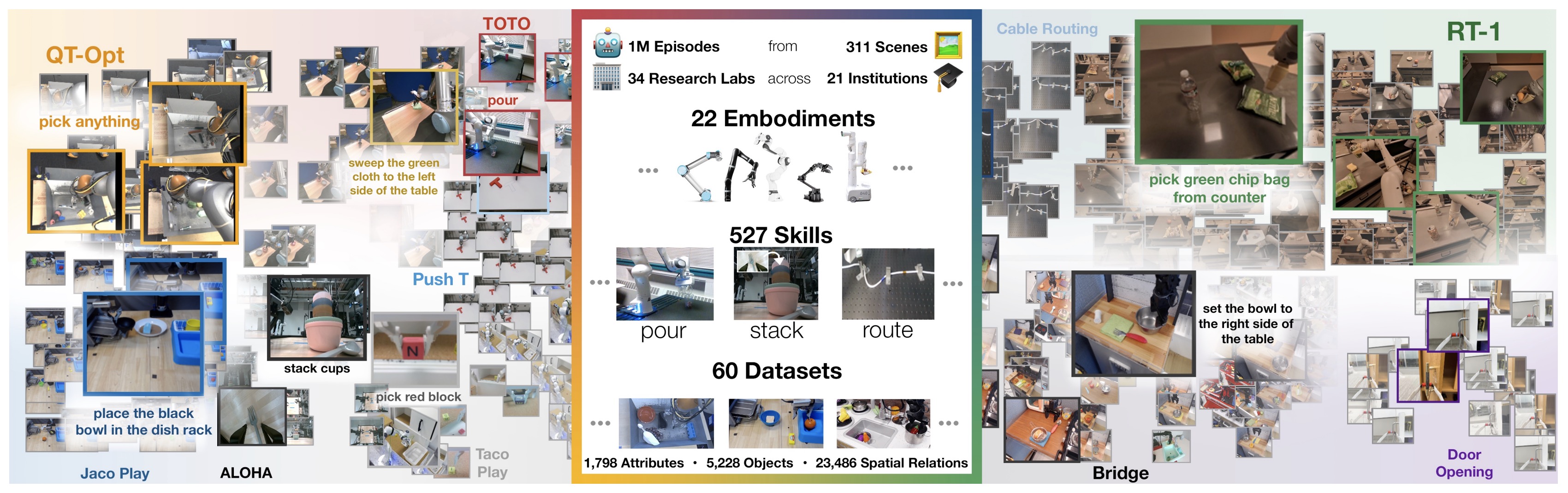
The following figure (source) illustrates this approach through the Open X-Embodiment dataset, which aggregates robot demonstrations from 21 institutions and spans a wide range of robot platforms, behaviors, and environments.

Suppose robot $i$ produces demonstrations $\mathcal{D}_i = \{(o_t^{(i)},a_t^{(i)},g^{(i)})\}$. Cross-embodiment training attempts to learn:
\[\pi_\theta \sim \bigcup_{i=1}^{N} \mathcal{D}_i\]
The challenge is that $\mathcal{A}_i \neq \mathcal{A}_j$ in general. Robots differ in degrees of freedom, coordinate systems, grippers, cameras, control rates, and kinematics. Open X-Embodiment: Robotic Learning Datasets and RT-X Models by Open X-Embodiment Collaboration et al. (2023) addresses this problem by standardizing heterogeneous datasets from 22 robot embodiments into a shared format and training RT-X models across the resulting mixture.
This introduces an important distinction between semantic universality and motor universality. Semantic concepts such as $\text{"pick up the cup"}$ can be shared broadly. The actual motor realization $a_{1:T}^{(i)}$ remains embodiment dependent.
A scalable Physical AI system therefore needs some combination of:
\[\text{shared semantics} + \text{shared physical representations} + \text{embodiment-specific adaptation}\]

Generalization as the Central Objective

Generalization as the Central Objective tests whether a policy can apply learned manipulation concepts to unseen instances or categories without relying on memorized appearance or object-specific trajectories.
Generalization as the Central Objective should report the task distribution, trial protocol, failure criteria, and interaction budget explicitly so improvements can be attributed to capability rather than easier scenarios or hidden assistance.
Embodied intelligence is ultimately a problem of generalization under interaction. This is the point where learned predictions meet coordinate frames, control rates, actuator limits, and the closed-loop dynamics of the physical system.
A useful decomposition is
\[G = \{ G_{\mathrm{object}}, G_{\mathrm{task}}, G_{\mathrm{scene}}, G_{\mathrm{language}}, G_{\mathrm{embodiment}}, G_{\mathrm{dynamics}} \}\]
An increasingly difficult sequence might be:
\[\text{known task + known object}\\ \downarrow\\ \text{known task + novel object}\\ \downarrow\\ \text{novel task composition}\\ \downarrow\\ \text{novel environment}\\ \downarrow\\ \text{novel embodiment}\\ \downarrow\\ \text{open-world physical autonomy}\]
VIMA explicitly evaluates increasingly difficult levels of generalization over multimodal manipulation prompts, while BC-Z investigates zero-shot task generalization and Open X-Embodiment examines transfer across robot datasets and embodiments. For embodied use, that semantic interpretation must remain tied to the current scene, the robot state, and the actions that are actually feasible for the embodiment.
These are not independent capabilities. General-purpose Physical AI requires them simultaneously.

The Emerging Embodied Foundation-Model Stack

The Emerging Embodied Foundation-Model Stack defines which parts of perception, reasoning, and control share a pretrained representation and which remain specialized, a boundary that governs transfer, latency, interpretability, and embodiment adaptation.
The Emerging Embodied Foundation-Model Stack should distinguish broadly reusable semantic and perceptual representations from robot-specific calibration in kinematics, dynamics, sensing, action ranges, and recovery behavior.
The evolution from classical robotics toward embodied foundation models can now be summarized as several architectural transitions. The design choice determines how much semantic knowledge can be shared across tasks while still preserving the precision and timing required by the robot-specific action interface.
First, perception shifted from task-specific visual pipelines toward reusable pretrained representations:
\[\text{task-specific vision} \rightarrow \text{foundation representations}\]
Second, task identity moved from separate policy weights into prompts:
\[\pi_{\theta,k}(a\mid o) \rightarrow \pi_\theta(a\mid o,g)\]
Third, robot control shifted from specialized architectures toward scalable sequence models:
\[\text{specialized policy} \rightarrow \text{Transformer policy}\]
Fourth, semantic reasoning became increasingly grounded in physical observations:
\[\text{LLM} \rightarrow \text{embodied multimodal model}\]
Finally, actions themselves became outputs of foundation models:
\[\text{VLM} \rightarrow \text{VLA}\]
Together these developments produce the modern embodied Physical AI stack:
\[\boxed{ \begin{array}{c} \text{Language / Goal / Prompt}\\ \downarrow\\ \text{Multimodal Perception}\\ \downarrow\\ \text{Semantic + Spatial Representation}\\ \downarrow\\ \text{Reasoning / Task Planning}\\ \downarrow\\ \text{Action Policy}\\ \downarrow\\ \text{Robot Controller}\\ \downarrow\\ \text{Physical World}\\ \circlearrowleft \end{array} }\]
The key research question has consequently shifted. The problem is no longer simply how to make a robot execute a particular behavior. It is how to construct models that can acquire broad knowledge from heterogeneous data, ground that knowledge through physical interaction, transfer it across tasks and embodiments, and reliably convert high-level intent into temporally coherent actions.
The next section will build directly on these foundations by examining “Learning to Act”: behavioral cloning, imitation learning, offline and online reinforcement learning, action chunking, diffusion and flow-matching policies, hierarchical control, and the training objectives used to turn demonstrations and interaction into executable physical behavior.

Learning to Act

Learning a useful policy requires choosing both a supervision signal and an action representation. This chapter connects imitation learning, generative action modeling, reinforcement learning, and deployment tradeoffs.

Imitation Learning and Action Representations

This section develops from understanding the world to controlling it in the context of the broader Physical AI system. It connects the underlying concepts to the implementation details discussed below.

From Understanding the World to Controlling It

A representation becomes useful for control only when it supports decisions about what to do next, so the transition from perception to policy requires grounding semantic features in state, dynamics, and action consequences.
From Understanding the World to Controlling It must be analyzed as part of the timed execution path from observation to actuation, because stale state, wrong frames, or delayed commands can invalidate an otherwise accurate prediction.
Perception and reasoning are useful only insofar as an embodied agent can convert them into successful physical behavior. The central learning problem in Physical AI is therefore to construct a policy
\[\pi_\theta(a_t \mid o_{\leq t}, g)\]
- that maps observations $o_{\leq t}$ and a goal $g$ into actions $a_t$.
The difficulty is that physical action spaces are fundamentally different from text. They are typically continuous, high-dimensional, temporally correlated, multimodal, embodiment-specific, and constrained by dynamics.
A robot may need to predict
\[a_t = [ \Delta x_t, \Delta y_t, \Delta z_t, \Delta r_t, \Delta p_t, \Delta y_t^{\mathrm{rot}}, g_t ]\]
- while a humanoid might simultaneously control dozens of joints.
The learning problem is therefore not merely:
\[\text{What action is correct?}\]
- but rather:
  \[\text{What coherent sequence of physically executable actions will achieve the goal?}\]
Modern Physical AI approaches this problem through several increasingly powerful paradigms:
\[\boxed{ \text{Behavioral Cloning} \rightarrow \text{Generative Policies} \rightarrow \text{Offline RL} \rightarrow \text{Online RL} \rightarrow \\ \text{Model-Based / World-Model Learning} }\]
These approaches are complementary rather than mutually exclusive. A modern robot foundation model can be pretrained by imitation, represented using a diffusion or flow-matching action head, and subsequently improved through reinforcement learning.

Behavioral Cloning

Behavioral Cloning learns directly from demonstrated observation-action pairs, but robust deployment depends on whether those demonstrations cover the states the policy will reach after its own inevitable small errors.
Behavioral cloning should therefore be evaluated beyond one-step imitation error, with particular attention to how errors compound when the learned policy controls its own future state distribution.
The simplest approach to learning physical behavior is behavioral cloning.
Suppose an expert generates demonstrations:
\[\mathcal{D} = \{ (o_t^{(i)},g^{(i)},a_t^{(i)}) \}_{i,t}\]
Behavioral cloning treats policy learning as supervised learning:
\[\theta^* = \arg\min_\theta \mathbb{E}_{(o,g,a)\sim\mathcal{D}} [ \mathcal{L}( \pi_\theta(o,g), a ) ]\]
For a probabilistic policy:
\[\mathcal{L}_{\mathrm{BC}} = - \mathbb{E}_{(o,g,a)\sim\mathcal{D}} [ \log \pi_\theta(a\mid o,g) ]\]
For deterministic continuous actions, a simple implementation can use:
\[\mathcal{L}_{\mathrm{MSE}} = \mathbb{E} \left[ \| a-\hat a_\theta(o,g) \|_2^2 \right]\]
The appeal of behavioral cloning is considerable. Robot demonstrations can be converted directly into supervised examples, and training can use the same large-scale optimization infrastructure as other foundation models. Learning Fine-Grained Bimanual Manipulation with Low-Cost Hardware by Zhao et al. (2023) demonstrates how imitation learning combined with temporal action prediction can produce precise bimanual manipulation from human demonstrations.
However, behavioral cloning contains two fundamental limitations: distribution shift and multimodality.

Distribution Shift and Compounding Errors

Distribution Shift and Compounding Errors becomes important because deployment changes the state distribution seen by the policy. Errors that are individually small can move the system into unfamiliar states, so robust control requires either broader data coverage, corrective examples, explicit recovery behavior, or online mechanisms that can re-establish a familiar state.
Distribution shift becomes consequential because small policy errors move the robot into states absent from the expert data, after which subsequent predictions are conditioned on increasingly unfamiliar observations.
The demonstrations in behavioral cloning are collected under the expert policy:
\[s_t \sim d^{\pi_E}(s)\]
Deployment instead produces states according to the learned policy:
\[s_t \sim d^{\pi_\theta}(s)\]
Even if $\pi_\theta(a\mid s) \approx \pi_E(a\mid s)$ on the training distribution, small errors alter subsequent states.
Suppose the expert follows
\[s_0 \xrightarrow{a_0^*} s_1^* \xrightarrow{a_1^*} s_2^*\]
The learned policy may instead execute:
\[s_0 \xrightarrow{\hat a_0} \hat s_1\]
If $\hat s_1 \notin \operatorname{support}(\mathcal{D})$, the next action prediction is now made from an unfamiliar state.
Errors can therefore compound:
\[\epsilon_1 \rightarrow \Delta s_1 \rightarrow \epsilon_2 \rightarrow \Delta s_2 \rightarrow \cdots\]
This problem motivated interactive imitation-learning methods such as DAgger, which repeatedly deploy a learned policy and request expert labels on states that the learner itself encounters. The resulting dataset increasingly approximates the learner’s deployment distribution rather than only the original expert distribution.
The underlying principle remains important for modern Physical AI:
\[\boxed{ \text{training data should cover states induced by the learned policy} }\]
- rather than exclusively states generated by successful expert demonstrations.

Why Mean-Squared Error Can Fail for Physical Actions

Pointwise regression can average across distinct valid behaviors, motivating objectives that represent multimodal action distributions rather than collapsing them into a single mean trajectory.
Why Mean-Squared Error Can Fail for Physical Actions should be evaluated through the behavior it produces after integration, because component-level metrics can miss timing, state-distribution, and control-interface failures that only appear in closed-loop execution.
Physical behavior is frequently multimodal.
Consider a robot moving around an obstacle. Two demonstrations may be equally valid:
\[a^{(1)} = \text{move left}\] \[a^{(2)} = \text{move right}\]
A deterministic regression model minimizing $\mathcal{L}_{\mathrm{MSE}} = \| a-\hat a \|^2$ is encouraged to predict the conditional mean:
\[\hat a = \mathbb{E}[a\mid o]\]
For a multimodal action distribution, the mean may correspond to no successful behavior:
\[\frac{1}{2} a^{(1)} + \frac{1}{2} a^{(2)} = \text{move directly toward obstacle}\]
Thus,
\[\boxed{ \text{average of valid actions} \neq \text{valid action} }\]
- in many physical control problems.
This observation motivates generative action models that represent the complete conditional distribution
\[p(a\mid o,g)\]
- rather than predicting a single point estimate.

Action Chunking

Action Chunking predicts multiple temporally coupled actions together, improving motion coherence and amortizing inference while trading away some per-timestep responsiveness.
Action Chunking changes how the policy represents and executes motion, so the chosen temporal horizon and action parameterization must remain compatible with controller rate, embodiment limits, and opportunities for feedback correction.
Physical actions are also strongly correlated through time. This is the point where learned predictions meet coordinate frames, control rates, actuator limits, and the closed-loop dynamics of the physical system.
Instead of predicting $a_t = \pi_\theta(o_t)$, a policy can generate an action chunk:
\[A_t = [ a_t, a_{t+1}, \ldots, a_{t+H-1} ]\]
The policy becomes:
\[A_t \sim \pi_\theta( A_t \mid o_{\leq t},g )\]
Learning Fine-Grained Bimanual Manipulation with Low-Cost Hardware by Zhao et al. (2023) introduced Action Chunking with Transformers, or ACT, which predicts temporally coherent action sequences rather than independently predicting every low-level command. Action chunking provides several advantages.
First, it captures temporal structure:
\[a_t \not\perp a_{t+1}\]
Second, it reduces the effective planning horizon. A task requiring $T$ low-level actions becomes approximately
\[\frac{T}{H}\]
- high-level prediction decisions when chunks of length $H$ are used.
Third, the model can represent coherent motion primitives such as
\[\text{approach} \rightarrow \text{grasp} \rightarrow \text{lift}\]
- rather than reconstructing the intended trajectory independently at every control cycle.

Receding-Horizon Execution

Receding-Horizon Execution repeatedly executes only part of a predicted action sequence before replanning from a new observation, balancing the smoothness of multi-step prediction with feedback-driven correction.
Receding-Horizon Execution should be evaluated through the behavior it produces after integration, because component-level metrics can miss timing, state-distribution, and control-interface failures that only appear in closed-loop execution.
Predicting an entire action sequence does not mean executing the entire sequence blindly. This is the point where learned predictions meet coordinate frames, control rates, actuator limits, and the closed-loop dynamics of the physical system.
Suppose the model predicts:
\[A_t = [a_t,\ldots,a_{t+H-1}]\]
The controller may execute only the first $K$ actions with $K < H$, then observe the environment again and replan:
\[o_t \xrightarrow{\pi} A_t \xrightarrow{\text{execute first }K} o_{t+K} \xrightarrow{\pi} A_{t+K}\]
This is receding-horizon control.
It combines the temporal coherence of action chunks with the robustness of feedback:
\[\boxed{ \text{long prediction horizon} + \text{short execution horizon} }\]
Diffusion Policy: Visuomotor Policy Learning via Action Diffusion by Chi et al. (2023) makes receding-horizon execution a central component of its visuomotor policy architecture, combining action-sequence generation with repeated visual feedback.

Action Chunking and Generative Policies

This section connects action chunking with transformers with diffusion policies. The discussion develops the relevant methods, implementation details, and practical tradeoffs.

Action Chunking with Transformers

Action Chunking with Transformers uses sequence modeling to predict a short block of coordinated actions, reducing the need to reconstruct the same motion intention independently at every control timestep.
Action Chunking with Transformers changes how the policy represents and executes motion, so the chosen temporal horizon and action parameterization must remain compatible with controller rate, embodiment limits, and opportunities for feedback correction.
ACT models action sequences using a conditional variational autoencoder. This is the point where learned predictions meet coordinate frames, control rates, actuator limits, and the closed-loop dynamics of the physical system.
The following figure (source) shows the ACT conditional-VAE architecture, including the training encoder and the action-chunk prediction decoder. Left: The encoder of the CVAE compresses action sequence and joint observation into z, the style variable. The encoder is discarded at test time. Right: The decoder or policy of ACT synthesizes images from multiple viewpoints, joint positions, and $z$with a transformer encoder, and predicts a sequence of actions with a transformer decoder. $z$is simply set to the mean of the prior (i.e. zero) at test time.

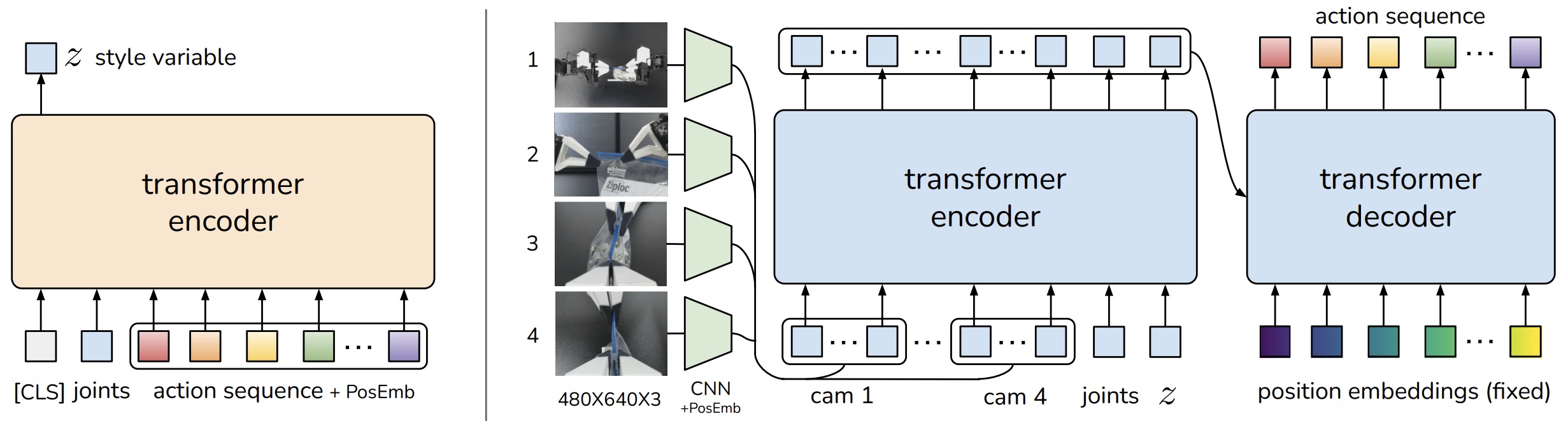
During training, an encoder receives the demonstration action sequence and contextual observations and infers a latent variable
\[z \sim q_\phi( z\mid A_t,o_t )\]
The decoder predicts the action chunk:
\[\hat A_t = f_\theta( o_t,z )\]
A simplified objective is:
\[\mathcal{L}_{\mathrm{ACT}} = \mathcal{L}_{\mathrm{reconstruction}} + \beta D_{\mathrm{KL}} \left( q_\phi(z\mid A_t,o_t) \| p(z) \right)\]
The latent variable captures variability in demonstrations, while the transformer models relationships across observations, robot state, and the future action sequence. In practice, the representation must preserve the task-relevant geometry, state, and uncertainty needed by downstream reasoning and control rather than only semantic appearance.
This approach is particularly useful for teleoperated demonstrations, where human behavior can exhibit substantial timing and trajectory variation even when the task outcome is identical. This is the point where learned predictions meet coordinate frames, control rates, actuator limits, and the closed-loop dynamics of the physical system.

Diffusion Policies

Diffusion Policies models a conditional distribution over continuous action sequences, making multimodal demonstrations and several valid motion strategies representable without averaging them into an invalid mean action.
Diffusion Policies changes how the policy represents and executes motion, so the chosen temporal horizon and action parameterization must remain compatible with controller rate, embodiment limits, and opportunities for feedback correction.
Diffusion models provide a more expressive solution to multimodal action generation. This is the point where learned predictions meet coordinate frames, control rates, actuator limits, and the closed-loop dynamics of the physical system.
The following figure (source) shows the diffusion-policy formulation and CNN/Transformer variants for denoising observation-conditioned action sequences.

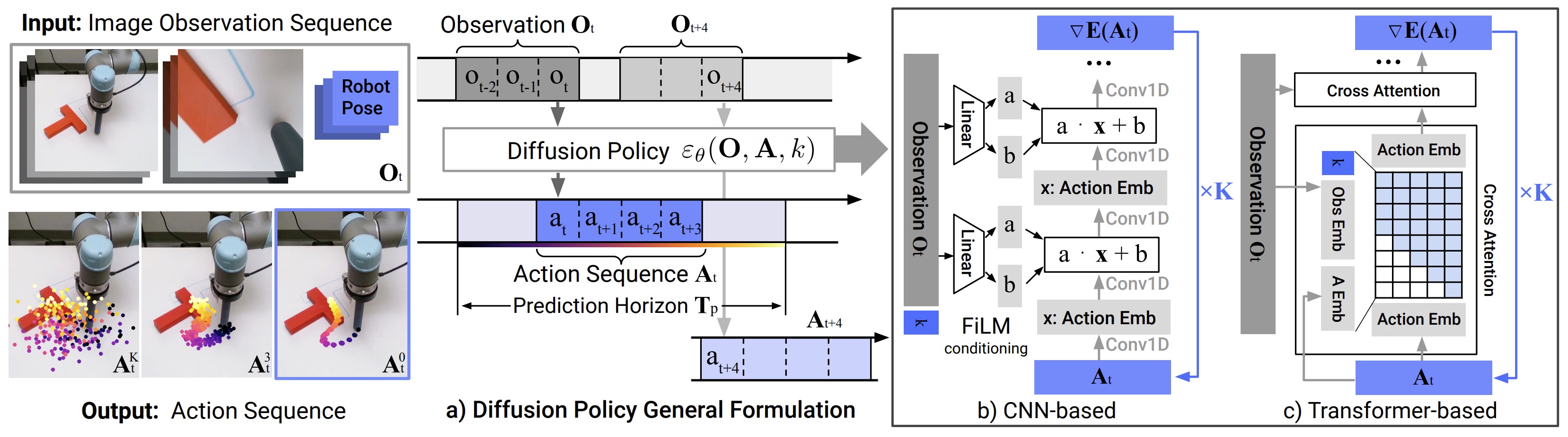
Diffusion Policy: Visuomotor Policy Learning via Action Diffusion by Chi et al. (2023) formulates robot policy learning as conditional denoising diffusion over action trajectories, demonstrating strong performance across diverse manipulation benchmarks and highlighting multimodal action modeling, high-dimensional control, and training stability as key advantages.
Instead of directly predicting $A_t = f_\theta(o_t)$, Diffusion Policy begins with noise $A_t^{K} \sim \mathcal{N}(0,I)$ and iteratively denoises it:
\[A_t^{K} \rightarrow A_t^{K-1} \rightarrow \cdots \rightarrow A_t^0\]
The final sample $A_t^0$ is the predicted action trajectory. This is the point where learned predictions meet coordinate frames, control rates, actuator limits, and the closed-loop dynamics of the physical system.
During training, noise is added to an expert action sequence:
\[A^k = \sqrt{\bar\alpha_k}A^0 + \sqrt{1-\bar\alpha_k}\epsilon\]
- where:
  \[\epsilon\sim\mathcal{N}(0,I)\]
The network learns to predict the noise:
\[\epsilon_\theta ( A^k, k, o )\]
A standard diffusion objective is:
\[\mathcal{L}_{\mathrm{diff}} = \mathbb{E}_{A^0,\epsilon,k} \left[ \| \epsilon - \epsilon_\theta( A^k,k,o ) \|_2^2 \right]\]
At inference time, iterative denoising generates an action trajectory conditioned on the current observation. In practice, the representation must preserve the task-relevant geometry, state, and uncertainty needed by downstream reasoning and control rather than only semantic appearance.

Why Diffusion Works Well for Robot Actions

Why Diffusion Works Well for Robot Actions benefits from diffusion’s ability to represent several valid action modes and denoise entire action sequences jointly, avoiding the averaging behavior of unimodal regression losses.
Why Diffusion Works Well for Robot Actions changes how the policy represents and executes motion, so the chosen temporal horizon and action parameterization must remain compatible with controller rate, embodiment limits, and opportunities for feedback correction.
Diffusion models have several properties that align naturally with physical control. This is the point where learned predictions meet coordinate frames, control rates, actuator limits, and the closed-loop dynamics of the physical system.

Multimodality

A diffusion policy can represent $p(A\mid o)$ with several distinct modes rather than averaging incompatible trajectories.

High-dimensional outputs

An action chunk can be represented as:
\[A \in \mathbb{R}^{H\times d_a}\]
For a humanoid or bimanual robot, both $H$ and $d_a$ can be large. Diffusion models can generate the complete structured object jointly.

Temporal coherence

The policy models $p(a_t, a_{t+1}, \ldots, a_{t+H} \mid o)$ rather than treating actions as conditionally independent.

Stable supervised training

Diffusion policy training remains essentially supervised learning over demonstration trajectories, avoiding many optimization instabilities associated with online reinforcement learning. This is the point where learned predictions meet coordinate frames, control rates, actuator limits, and the closed-loop dynamics of the physical system.
The tradeoff is inference cost. A diffusion policy may require several network evaluations to produce one action sequence, so the number of denoising steps directly affects control frequency and compute requirements.

Diffusion Transformers for Large Robot Policies

Diffusion Transformers for Large Robot Policies uses transformer capacity inside a generative action model to condition continuous trajectory generation on multimodal context while preserving temporal dependencies across the predicted action horizon.
Diffusion Transformers for Large Robot Policies changes how the policy represents and executes motion, so the chosen temporal horizon and action parameterization must remain compatible with controller rate, embodiment limits, and opportunities for feedback correction.
The combination of diffusion objectives with transformer backbones naturally extends to foundation-scale robot models. The training stage should therefore be interpreted by the capability it is intended to add: broad representations, embodiment grounding, task adaptation, or closed-loop behavioral improvement.
RDT-1B: a Diffusion Foundation Model for Bimanual Manipulation by Liu et al. (2024) scales a Robotics Diffusion Transformer to approximately 1.2B parameters, introduces a physically interpretable unified action representation across robots, and pretrains on heterogeneous multi-robot data before task-specific fine-tuning.
A generic architecture is:
\[z_{\mathrm{vision}} = f_{\mathrm{vision}}(I)\] \[z_{\mathrm{text}} = f_{\mathrm{text}}(g)\] \[z_{\mathrm{state}} = f_{\mathrm{state}}(s)\]
- followed by:
  \[\epsilon_\theta = \operatorname{DiT} ( A^k, k, z_{\mathrm{vision}}, z_{\mathrm{text}}, z_{\mathrm{state}} )\]
The Diffusion Transformer therefore functions as an action expert conditioned on representations supplied by perception and language systems. In practice, the representation must preserve the task-relevant geometry, state, and uncertainty needed by downstream reasoning and control rather than only semantic appearance.

From Diffusion to Flow Matching

From Diffusion to Flow Matching learns a continuous transport field from a simple base distribution to robot action trajectories, providing a multimodal action decoder that can often be sampled with fewer integration steps than diffusion.
From Diffusion to Flow Matching changes how the policy represents and executes motion, so the chosen temporal horizon and action parameterization must remain compatible with controller rate, embodiment limits, and opportunities for feedback correction.
Flow matching learns a continuous vector field that transports samples from a simple source distribution to the target action distribution. This is the point where learned predictions meet coordinate frames, control rates, actuator limits, and the closed-loop dynamics of the physical system.
Let $x_0\sim p_0$ be noise and $x_1\sim p_{\mathrm{data}}$ be an expert action trajectory. A simple interpolation is:
\[x_\tau = (1-\tau)x_0+\tau x_1, \qquad \tau\in[0,1]\]
The target velocity is:
\[u_\tau=x_1-x_0\]
A neural network learns:
\[v_\theta(x_\tau,\tau,c)\approx u_\tau\]
- where $c$ contains conditioning information such as images, language, and robot state.
The flow-matching objective can be written:
\[\mathcal{L}_{\mathrm{FM}} = \mathbb{E} \left[ \| v_\theta(x_\tau,\tau,c)-u_\tau \|_2^2 \right]\]
At inference time, actions are generated by integrating:
\[\frac{dx}{d\tau} = v_\theta(x,\tau,c)\]
- from noise toward the learned action distribution.

Flow Matching in Modern VLAs

Flow Matching in Modern VLAs learns a continuous transport field from a simple base distribution to robot action trajectories, providing a multimodal action decoder that can often be sampled with fewer integration steps than diffusion.
Flow Matching in Modern VLAs changes how the policy represents and executes motion, so the chosen temporal horizon and action parameterization must remain compatible with controller rate, embodiment limits, and opportunities for feedback correction.
$\pi_0$: A Vision-Language-Action Flow Model for General Robot Control by Black et al. (2024) applies flow matching to robot action generation, combining a pretrained vision-language model with a dedicated action expert that produces continuous action chunks.
The key architectural separation is
\[\text{VLM} \rightarrow \text{semantic representation}\] \[\text{action expert} \rightarrow \text{continuous control}\]
The successor $\pi_{0.5}$: a Vision-Language-Action Model with Open-World Generalization by Black et al. (2025) extends this approach with heterogeneous co-training across robot data, web data, semantic subtasks, object detections, and low-level actions to improve long-horizon generalization in unfamiliar environments.

Diffusion Versus Flow Matching

Diffusion Versus Flow Matching compares two continuous generative parameterizations: diffusion learns iterative denoising, while flow matching learns a vector field that transports samples toward the action distribution, with different sampling-cost and training tradeoffs.
Diffusion Versus Flow Matching changes how the policy represents and executes motion, so the chosen temporal horizon and action parameterization must remain compatible with controller rate, embodiment limits, and opportunities for feedback correction.
At a high level, both approaches learn generative action distributions:
\[p_\theta(A\mid o,g)\]
Diffusion commonly learns a denoising or score function and solves a reverse stochastic process, while flow matching learns a velocity field and solves an ODE. For control, the benefit is the ability to represent multimodal temporally coherent action distributions, while inference cost and replanning cadence remain deployment constraints.
Conceptually:
\[\text{Diffusion}:\text{ iterative denoising}\] \[\text{Flow Matching}:\text{ continuous transport}\]
Both are attractive for Physical AI because they naturally model multimodal, high-dimensional action sequences. This is the point where learned predictions meet coordinate frames, control rates, actuator limits, and the closed-loop dynamics of the physical system.

Reinforcement Learning

This section connects why imitation alone is not enough with value functions and physical decision making. The discussion develops the relevant methods, implementation details, and practical tradeoffs.

Why Imitation Alone Is Not Enough

Why Imitation Alone Is Not Enough follows from covariate shift: a policy trained only on expert states eventually encounters its own off-trajectory states, where supervised demonstrations provide progressively weaker guidance.
Why Imitation Alone Is Not Enough should be evaluated through the behavior it produces after integration, because component-level metrics can miss timing, state-distribution, and control-interface failures that only appear in closed-loop execution.
Imitation learning asks:
\[\text{What did the demonstrator do?}\]
Reinforcement learning asks:
\[\text{What behavior maximizes the objective?}\]
The reinforcement-learning objective is:
\[J(\pi) = \mathbb{E}_{\tau\sim\pi} \left[ \sum_{t=0}^{T} \gamma^t r(s_t,a_t) \right]\]
Rather than matching actions, the policy is optimized for consequences. This makes RL particularly attractive for post-training a Physical AI model that already possesses useful behavior from imitation learning.

Value Functions and Physical Decision Making

Value Functions and Physical Decision Making uses reward or value information to distinguish better and worse actions without requiring unrestricted online exploration. Its reliability depends on how far policy improvement moves beyond the support of the logged data, because value estimates become less trustworthy for actions or states that were rarely observed.
Value Functions and Physical Decision Making depends on the feedback channel available during adaptation: offline supervision favors conservative updates within known data, whereas interactive feedback can correct new failure states at the cost of additional exploration and safety management.
The action-value function is:
\[Q^\pi(s,a) = \mathbb{E}_\pi \left[ \sum_{k=0}^{\infty} \gamma^k r_{t+k} \mid s_t=s,a_t=a \right]\]
The state-value function is:
\[V^\pi(s) = \mathbb{E}_{a\sim\pi}[Q^\pi(s,a)]\]
The advantage function is:
\[A^\pi(s,a)=Q^\pi(s,a)-V^\pi(s)\]
These functions allow robot learning to move beyond pure imitation by preferring actions associated with higher eventual success. This is the point where learned predictions meet coordinate frames, control rates, actuator limits, and the closed-loop dynamics of the physical system.

Offline Reinforcement Learning

Offline Reinforcement Learning uses reward or value information to distinguish better and worse actions without requiring unrestricted online exploration. Its reliability depends on how far policy improvement moves beyond the support of the logged data, because value estimates become less trustworthy for actions or states that were rarely observed.
Offline Reinforcement Learning is constrained by the support of the logged dataset, so optimization must improve decisions without assigning unwarranted value to actions that were rarely or never observed.
Real-world robot interaction is expensive and potentially dangerous. Physical AI therefore often begins with static datasets
\[\mathcal{D} = \{(s_t,a_t,r_t,s_{t+1})\}\]
Offline RL attempts to improve a policy using this fixed dataset without additional environment interaction. This is the point where learned predictions meet coordinate frames, control rates, actuator limits, and the closed-loop dynamics of the physical system.
The central challenge is extrapolation. A learned Q-function may assign high value to actions absent from the dataset:
\[a_{\mathrm{OOD}}\notin\mathcal{D}\]
Because estimates for such actions are poorly constrained, maximizing $Q_\theta(s,a)$ can select actions whose apparent value results from function-approximation error. This is the point where learned predictions meet coordinate frames, control rates, actuator limits, and the closed-loop dynamics of the physical system.

Conservative Q-Learning

Conservative Q-Learning uses reward or value information to distinguish better and worse actions without requiring unrestricted online exploration. Its reliability depends on how far policy improvement moves beyond the support of the logged data, because value estimates become less trustworthy for actions or states that were rarely observed.
Conservative Q-Learning is constrained by the support of the logged dataset, so optimization must improve decisions without assigning unwarranted value to actions that were rarely or never observed.
Conservative Q-Learning for Offline Reinforcement Learning by Kumar et al. (2020) addresses offline-RL distribution shift by penalizing high Q-values for actions unsupported by the dataset.
A simplified objective is:
\[\mathcal{L}_{\mathrm{CQL}} = \mathcal{L}_{\mathrm{Bellman}} + \alpha \left[ \mathbb{E}_{s}\log\sum_a\exp Q(s,a) - \mathbb{E}_{(s,a)\sim\mathcal{D}}Q(s,a) \right]\]
The intuition is:
\[\boxed{ \text{do not trust apparently excellent actions that the data cannot support} }\]

Implicit Q-Learning

Implicit Q-Learning uses reward or value information to distinguish better and worse actions without requiring unrestricted online exploration. Its reliability depends on how far policy improvement moves beyond the support of the logged data, because value estimates become less trustworthy for actions or states that were rarely observed.
Implicit Q-Learning is constrained by the support of the logged dataset, so optimization must improve decisions without assigning unwarranted value to actions that were rarely or never observed.
Offline Reinforcement Learning with Implicit Q-Learning by Kostrikov et al. (2021) avoids evaluating unseen actions during policy improvement, using expectile regression to estimate high-value behavior within the support of the offline dataset.
IQL fits the value function using:
\[\mathcal{L}_V = \mathbb{E}_{(s,a)\sim\mathcal{D}} [ L_\tau^2(Q(s,a)-V(s)) ]\]
- where:
  \[L_\tau^2(u) = |\tau-\mathbb{1}(u<0)|u^2\]
Policy extraction resembles advantage-weighted behavioral cloning:
\[\mathcal{L}_{\pi} = - \mathbb{E}_{(s,a)\sim\mathcal{D}} \left[ \exp(\beta A(s,a)) \log\pi_\theta(a\mid s) \right]\]
The practical interpretation is:
\[\text{imitate the dataset} + \text{prefer its better behaviors}\]

Advantage-Weighted Policy Learning

Advantage-Weighted Policy Learning uses reward or value information to distinguish better and worse actions without requiring unrestricted online exploration. Its reliability depends on how far policy improvement moves beyond the support of the logged data, because value estimates become less trustworthy for actions or states that were rarely observed.
Advantage-Weighted Policy Learning is constrained by the support of the logged dataset, so optimization must improve decisions without assigning unwarranted value to actions that were rarely or never observed.
Advantage-Weighted Regression: Simple and Scalable Off-Policy Reinforcement Learning by Peng et al. (2019) formulates policy learning as weighted maximum likelihood with weights determined by estimated advantages.
A typical objective is:
\[\mathcal{L}_{\mathrm{AWR}} = - \mathbb{E}_{(s,a)\sim\mathcal{D}} [ w(s,a)\log\pi_\theta(a\mid s) ]\]
- with:
  \[w(s,a)=\exp\left(\frac{A(s,a)}{\beta}\right)\]
This creates a useful bridge between imitation learning and RL because policy updates remain structurally similar to supervised post-training while incorporating reward information. This is the point where learned predictions meet coordinate frames, control rates, actuator limits, and the closed-loop dynamics of the physical system.

Hierarchical and Model-Based Control

This section connects online reinforcement learning with reward design. The discussion develops the relevant methods, implementation details, and practical tradeoffs.

Online Reinforcement Learning

Online Reinforcement Learning allows the policy to learn from the consequences of its own behavior rather than demonstrations alone. This can correct systematic imitation errors, but it also makes reward specification, exploration safety, reset cost, and intervention handling first-class parts of the training system.
Online Reinforcement Learning can discover useful behavior outside the offline dataset because the policy collects new experience, but exploration cost and safety become part of the learning problem.
Online RL allows the policy to interact with the environment:
\[\pi_\theta \rightarrow \tau \rightarrow r \rightarrow \text{update }\theta \rightarrow \pi_{\theta'}\]
This enables exploration and direct correction of policy-induced distribution shift, but real-world online RL faces sample cost, hardware wear, reset cost, safety risk, and human-supervision constraints. In practice, the representation must preserve the task-relevant geometry, state, and uncertainty needed by downstream reasoning and control rather than only semantic appearance.
Practical Physical AI systems often use a staged recipe:
\[\boxed{ \text{large-scale pretraining} \rightarrow \text{behavioral cloning} \rightarrow \text{offline RL} \rightarrow \text{simulation RL} \rightarrow \\ \text{limited real-world online RL} }\]

Reward Design

Reward Design allows the policy to learn from the consequences of its own behavior rather than demonstrations alone. This can correct systematic imitation errors, but it also makes reward specification, exploration safety, reset cost, and intervention handling first-class parts of the training system.
Reward Design depends on the feedback channel available during adaptation: offline supervision favors conservative updates within known data, whereas interactive feedback can correct new failure states at the cost of additional exploration and safety management.
For a manipulation task, a sparse reward might be:
\[r_t = \begin{cases} 1 & \text{task completed}\\ 0 & \text{otherwise}. \end{cases}\]
A shaped reward may instead include:
\[r_t = w_1r_{\mathrm{reach}} + w_2r_{\mathrm{grasp}} + w_3r_{\mathrm{transport}} + w_4r_{\mathrm{success}} - w_5r_{\mathrm{collision}}\]
Reward shaping improves credit assignment but creates the possibility that optimizing the specified reward does not produce the intended behavior. Physical AI therefore increasingly combines simulator state, task-completion detectors, learned reward models, vision-language models, human feedback, and rule-based safety constraints.

Hierarchical Control

Hierarchical Control separates decisions that benefit from slower semantic reasoning from those that require fast, stable control. The boundary between these levels is operationally important: high-level modules should expose goals or constraints that remain meaningful long enough for the low-level controller to execute them.
Hierarchical Control must be analyzed as part of the timed execution path from observation to actuation, because stale state, wrong frames, or delayed commands can invalidate an otherwise accurate prediction.
Long-horizon tasks create enormous low-level action horizons. Hierarchical control introduces different temporal scales:
\[g \xrightarrow{\pi_{\mathrm{high}}} z_k \xrightarrow{\pi_{\mathrm{low}}} a_{t:t+H}\]
The high-level policy predicts subgoals or skills, while the low-level policy converts each skill into continuous actions. This separates the semantic horizon from the motor horizon.

System 2 and System 1 Control

System 2 and System 1 Control separates decisions that benefit from slower semantic reasoning from those that require fast, stable control. The boundary between these levels is operationally important: high-level modules should expose goals or constraints that remain meaningful long enough for the low-level controller to execute them.
System 2 and System 1 Control must be analyzed as part of the timed execution path from observation to actuation, because stale state, wrong frames, or delayed commands can invalidate an otherwise accurate prediction.
An increasingly useful abstraction for Physical AI is a two-timescale architecture. A slower reasoning system handles scene understanding, task decomposition, planning, and recovery reasoning. A faster motor system handles continuous trajectories, reactive control, and contact dynamics.
Conceptually,
\[\boxed{ \text{System 2} \xrightarrow{\text{subgoal}} \text{System 1} \xrightarrow{\text{actions}} \text{World} }\]
- with feedback returning to both systems.
This division is useful because high-level reasoning and low-level motor control have very different latency and compute requirements. In practice, the representation must preserve the task-relevant geometry, state, and uncertainty needed by downstream reasoning and control rather than only semantic appearance.

Model-Based Reinforcement Learning

Model-Based Reinforcement Learning supports reinforcement learning by producing imagined or simulated experience in which policies can explore consequences more cheaply than on hardware, subject to the risk of exploiting model errors.
Model-Based Reinforcement Learning depends on the feedback channel available during adaptation: offline supervision favors conservative updates within known data, whereas interactive feedback can correct new failure states at the cost of additional exploration and safety management.
Model-based RL learns or uses a transition model to predict how the environment evolves in response to actions, enabling the agent to plan using predicted outcomes. For example, TD-MPC2 learns a latent world model that predicts future states, rewards, and values without reconstructing future observations. Its transition model is expressed as:
\[\hat s_{t+1}=f_\phi(s_t,a_t)\]
The following figure (source) shows the TD-MPC2 latent world-model architecture, which predicts rewards and values without reconstructing future observations.

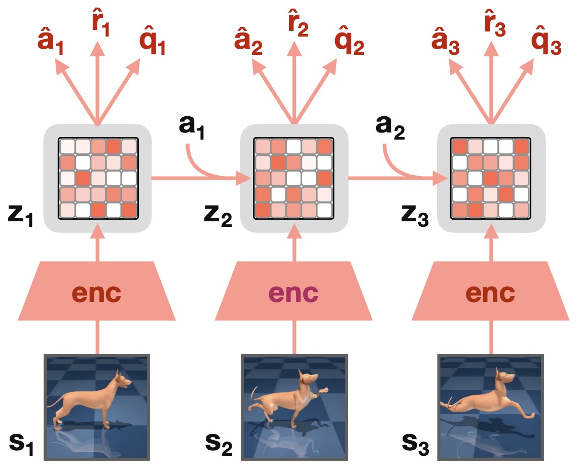
The agent can evaluate hypothetical futures:
\[s_t \xrightarrow{a_t} \hat s_{t+1} \xrightarrow{a_{t+1}} \hat s_{t+2} \rightarrow\cdots\]
An action sequence can be selected by maximizing predicted return:
\[a_{t:t+H}^* = \arg\max_{a_{t:t+H}} \sum_{k=0}^{H} \gamma^k \hat r(\hat s_{t+k},a_{t+k})\]
This creates the connection:
\[\boxed{ \text{learn dynamics} \rightarrow \text{imagine futures} \rightarrow \text{choose actions} }\]
- that underlies world-model-based Physical AI.

Latent World Models

Latent World Models predicts dynamics in a compressed state space, reducing rollout cost while relying on the latent representation to preserve the factors that change rewards and optimal actions.
Latent World Models is useful only if compression preserves the variables that change rewards and action rankings; high reconstruction quality is neither necessary nor sufficient for that decision-level requirement.
Instead of predicting raw future pixels, an encoder can map observations into latent states:
\[z_t=e_\phi(o_t)\]
- with learned latent dynamics:
  \[\hat z_{t+1}=f_\phi(z_t,a_t)\]
TD-MPC2: Scalable, Robust World Models for Continuous Control by Hansen et al. (2024) performs local trajectory optimization inside a learned decoder-free latent world model and demonstrates scaling across many continuous-control tasks and embodiments.
A simplified planning objective is:
\[A^* = \arg\max_A \left[ \sum_{k=0}^{H-1} \gamma^k R_\phi(z_k,a_k) + \gamma^H Q_\phi(z_H,a_H) \right]\]
The model need not reconstruct every pixel. It only needs a latent representation sufficiently accurate for evaluating actions.

Training in Simulation

Training in Simulation models how physical state evolves under actions, enabling counterfactual prediction, planning, synthetic experience, and closed-loop evaluation before every decision is attempted in the real world.
Training in Simulation should vary or calibrate the physical and sensing factors that materially affect the deployed policy, with success measured by transfer to held-out real behavior rather than by simulator performance alone.
One solution to the cost of physical interaction is to move reinforcement learning into simulation:
\[s_{t+1}^{\mathrm{sim}} = F_{\mathrm{sim}}(s_t^{\mathrm{sim}},a_t)\]
Simulation provides large-scale parallel rollouts, automatic resets, and privileged reward signals. Because each executed command changes the next input distribution, the relevant unit of evaluation is the resulting rollout rather than an isolated one-step prediction.
The central problem becomes sim-to-real transfer:
\[P_{\mathrm{sim}}(s'|s,a) \neq P_{\mathrm{real}}(s'|s,a)\]
Differences in friction, mass, lighting, sensor noise, actuator response, object geometry, and contact dynamics can cause policies trained in simulation to fail physically. This motivates domain randomization, system identification, digital twins, and learned world models.

Deployment and Adaptation

This section connects combining demonstrations and reinforcement learning with closed-loop policy improvement. The discussion develops the relevant methods, implementation details, and practical tradeoffs.

Combining Demonstrations and Reinforcement Learning

Combining Demonstrations and Reinforcement Learning combines the stable initialization of demonstrations with interactive optimization, allowing the policy to refine behavior in states that were missing or rare in the offline dataset.
Combining Demonstrations and Reinforcement Learning should be assessed by the new behavioral coverage it contributes, especially rare states, recovery situations, and observation-action combinations that are missing from the current training distribution.
A powerful Physical AI training recipe combines imitation and RL. What matters is not only the number of examples but also their coverage of tasks, embodiments, recovery states, and observation-action alignments that the deployed policy will encounter.
Start with expert demonstrations $\mathcal{D}_E$ train an initial policy:
\[\pi_0=\operatorname{BC}(\mathcal{D}_E)\]
- collect or generate policy experience $\mathcal{D}_\pi$, estimate outcome quality, and improve the policy while remaining near useful demonstrated behavior.
The pipeline becomes
\[\boxed{ \text{Demonstrations} \rightarrow \text{SFT / BC} \rightarrow \text{Rollouts} \rightarrow \text{Rewards} \rightarrow \text{RL Post-Training} \rightarrow \text{Improved Policy} }\]
This resembles post-training pipelines for language models, but the rollouts occur in physical or simulated environments and the outputs are actions rather than text. For embodied use, that semantic interpretation must remain tied to the current scene, the robot state, and the actions that are actually feasible for the embodiment.

Closed-Loop Policy Improvement

Closed-Loop Policy Improvement evaluates behavior through the feedback loop created when each action changes the next state and observation, exposing compounding errors that static prediction metrics can hide.
Closed-Loop Policy Improvement depends on the feedback channel available during adaptation: offline supervision favors conservative updates within known data, whereas interactive feedback can correct new failure states at the cost of additional exploration and safety management.
Deployment generates trajectories:
\[\tau_k\sim P(\tau\mid\pi_k)\]
Failures reveal weaknesses in the policy’s own state distribution. New training data can focus on:
\[\mathcal{D}_{k+1} = \mathcal{D}_k \cup \mathcal{D}_{\mathrm{failure}} \cup \mathcal{D}_{\mathrm{recovery}}\]
Retraining produces $\pi_{k+1}$, and the process repeats:
\[\boxed{ \pi_k \rightarrow \text{Deploy} \rightarrow \text{Observe Failures} \rightarrow \text{Collect Corrections} \rightarrow \text{Train} \rightarrow \pi_{k+1} }\]
The most valuable data is often concentrated near the current policy’s failure boundary. This is the point where learned predictions meet coordinate frames, control rates, actuator limits, and the closed-loop dynamics of the physical system.

Learning Recovery Behavior

Learning Recovery Behavior becomes important because deployment changes the state distribution seen by the policy. Errors that are individually small can move the system into unfamiliar states, so robust control requires either broader data coverage, corrective examples, explicit recovery behavior, or online mechanisms that can re-establish a familiar state.
Learning Recovery Behavior should report the task distribution, trial protocol, failure criteria, and interaction budget explicitly so improvements can be attributed to capability rather than easier scenarios or hidden assistance.
Robust autonomy requires behavior under off-nominal states, not merely successful demonstrations. What matters is not only the number of examples but also their coverage of tasks, embodiments, recovery states, and observation-action alignments that the deployed policy will encounter.
A robust policy should learn:
\[\pi(a_{\mathrm{recover}}\mid s_{\mathrm{off-nominal}})\]
- in addition to:
  \[\pi(a_{\mathrm{expert}}\mid s_{\mathrm{nominal}})\]
This suggests:
\[\boxed{ \text{competence} = \text{successful execution} + \text{failure detection} + \text{recovery} }\]
- as a more complete definition of long-horizon physical autonomy.

Action Representations

Action representation determines what the policy must learn: joint targets, end-effector deltas, trajectories, latent actions, and tokenized commands impose different invariances, temporal scales, and embodiment assumptions.
Action Representations changes how the policy represents and executes motion, so the chosen temporal horizon and action parameterization must remain compatible with controller rate, embodiment limits, and opportunities for feedback correction.
A policy might predict joint positions $a_t=q_t^*$ joint velocities $a_t=\dot q_t^*$ joint torques $a_t=\tau_t$ or Cartesian end-effector commands:
\[a_t=[\Delta x,\Delta R,g]\]
Lower-level actions expose more control but require the learned model to understand more dynamics. Higher-level actions simplify learning but rely more heavily on downstream controllers.
This creates a hierarchy:
\[\text{semantic skill} \rightarrow \text{Cartesian trajectory} \rightarrow \text{joint trajectory} \rightarrow \text{torque}\]
A foundation model does not necessarily need to operate at the bottom of this hierarchy. A useful plan therefore has to connect high-level intent to reachable intermediate states and leave room to replan when execution produces an unexpected observation.

Cross-Embodiment Action Spaces

Cross-Embodiment Action Spaces must reconcile robot-specific units, ranges, joint structures, and control conventions so a shared model can learn common behavior without confusing incompatible command semantics.
Cross-Embodiment Action Spaces must be analyzed as part of the timed execution path from observation to actuation, because stale state, wrong frames, or delayed commands can invalidate an otherwise accurate prediction.
Foundation models introduce the challenge:
\[\mathcal{A}_{\mathrm{robot\ A}} \neq \mathcal{A}_{\mathrm{robot\ B}}\]
RDT-1B addresses this with a physically interpretable unified action representation intended to preserve physical semantics while supporting heterogeneous robots. For embodied use, that semantic interpretation must remain tied to the current scene, the robot state, and the actions that are actually feasible for the embodiment.
More generally,
\[a_t^{(e)}=f_e(z_t)\]
- where $z_t$ is a shared latent action representation and $f_e$ maps that representation into embodiment-specific commands.
This separates what motion should occur from how a particular robot realizes that motion. This is the point where learned predictions meet coordinate frames, control rates, actuator limits, and the closed-loop dynamics of the physical system.

The Modern Action-Learning Stack

The Modern Action-Learning Stack defines which parts of perception, reasoning, and control share a pretrained representation and which remain specialized, a boundary that governs transfer, latency, interpretability, and embodiment adaptation.
The Modern Action-Learning Stack should be evaluated through the behavior it produces after integration, because component-level metrics can miss timing, state-distribution, and control-interface failures that only appear in closed-loop execution.
The evolution of learned control can be summarized as several transitions:
\[\text{single-action regression} \rightarrow \text{action chunking}\] \[\text{unimodal regression} \rightarrow \text{generative action distributions}\] \[\text{behavior cloning} \rightarrow \text{reward-aware policy improvement}\] \[\text{offline demonstrations} \rightarrow \text{closed-loop interaction}\] \[\text{model-free control} \rightarrow \text{world-model-assisted learning}\]
The resulting architecture increasingly resembles:
\[\boxed{ \begin{array}{c} \text{Multimodal Observation + Goal}\\ \downarrow\\ \text{Foundation Representation}\\ \downarrow\\ \text{High-Level Reasoning / Subgoal}\\ \downarrow\\ \text{Generative Action Expert}\\ \downarrow\\ \text{Action Chunk}\\ \downarrow\\ \text{Low-Level Controller}\\ \downarrow\\ \text{Physical Environment}\\ \downarrow\\ \text{Reward + New Observation}\\ \circlearrowleft \end{array} }\]
The central trend is a shift from learning a deterministic mapping from images to individual motor commands toward learning rich distributions over temporally extended behavior and improving those distributions using interaction. In practice, the representation must preserve the task-relevant geometry, state, and uncertainty needed by downstream reasoning and control rather than only semantic appearance.
This provides the algorithmic foundation for modern Vision-Language-Action models. The next section will examine those models directly, including RT-2, OpenVLA, Octo, $\pi_0$, $\pi_{0.5}$, tokenized versus continuous action representations, cross-embodiment training, and the engineering details required to turn a pretrained multimodal model into a generalist robot policy.
World-action models add another transition to this stack by fusing world-model-assisted learning with the action generator itself. Instead of maintaining a strict separation between a policy that proposes actions and a world model that predicts consequences, a WAM learns a joint conditional distribution over future observations and actions:
\[p_\theta\left(o_{t+1:t+H},a_{t:t+H}\mid o_{\leq t},s_{\leq t},g\right)\]
World Action Models are Zero-shot Policies by Ye et al. (2026) demonstrates this formulation with DreamZero, while FLUX 3 Action applies it to a 7B robot-control model. The resulting progression therefore extends beyond using a world model as an external planner:
\[\text{world-model-assisted policy} \rightarrow \text{joint world-action prediction}\]

Vision-Language-Action Models

Vision-Language-Action models connect multimodal understanding to executable robot behavior. The sections below compare tokenized and continuous policies, representative systems, and practical adaptation choices.
A detailed discourse on Vision-Language-Action models and World Models is offered in our World Models primer. In practice, the representation must preserve the task-relevant geometry, state, and uncertainty needed by downstream reasoning and control rather than only semantic appearance.

VLA Foundations

This section develops from vision-language models to physical policies in the context of the broader Physical AI system. It connects the underlying concepts to the implementation details discussed below.

From Vision-Language Models to Physical Policies

Converting a vision-language backbone into a physical policy requires more than attaching an action head: the learned representation must expose the spatial, temporal, and task-conditioned information needed to predict valid controls from the current robot state.
From Vision-Language Models to Physical Policies should connect semantic intent to the current physical state and available actions, with execution feedback used to verify that the chosen interpretation actually produced the intended effect.
Vision-Language-Action models, or VLAs, are one of the central architectural abstractions in modern Physical AI. They extend vision-language models by adding physically executable actions to the model’s output space.
A conventional vision-language model approximates:
\[p_\theta(y\mid I,l)\]
- where $I$ is an image, $l$ is a textual prompt, and $y$ is a textual response.
A VLA instead models
\[\pi_\theta(a\mid I,l,s)\]
- where $s$ may contain proprioceptive or other robot state and $a$ represents an executable action.
For temporally extended control, this becomes:
\[\pi_\theta( a_{t:t+H} \mid I_{\leq t}, s_{\leq t}, l )\]
The conceptual change appears small:
\[\boxed{ \text{Vision} + \text{Language} \rightarrow \text{Text} }\]
- becomes:
  \[\boxed{ \text{Vision} + \text{Language} + \text{Robot State} \rightarrow \text{Action} }\]
  - but this changes the role of the model fundamentally. Its predictions now participate directly in a closed-loop dynamical system.
RT-2: Vision-Language-Action Models Transfer Web Knowledge to Robotic Control by Brohan et al. (2023) formalized this VLA paradigm by co-fine-tuning pretrained vision-language models on both web-scale vision-language tasks and robot trajectories, representing robot actions in the same token vocabulary used for language.

Why Start from a Vision-Language Model?

Vision-language pretraining provides broad object, language, and relational knowledge that robot policies can reuse, reducing the amount of robot-specific data needed to learn semantics from scratch while leaving physical grounding and control to downstream adaptation.
Why Start from a Vision-Language Model? should connect semantic intent to the current physical state and available actions, with execution feedback used to verify that the chosen interpretation actually produced the intended effect.
A robot policy trained exclusively on robot demonstrations can only learn concepts represented in those demonstrations. Suppose $\mathcal{D}_{\mathrm{robot}}$ contains demonstrations involving cups, bowls, fruit, and utensils but no demonstration involving a dinosaur toy. A robot-only policy has little reason to understand the concept $\text{"dinosaur"}$. A VLM pretrained on internet-scale image-text data may already encode such knowledge.
The VLA hypothesis is therefore:
\[\boxed{ \text{Internet semantic knowledge} + \text{robot interaction data} \rightarrow \text{semantically capable physical policy}. }\]
The robot data teaches the model how semantic concepts map into physical actions, while vision-language pretraining provides much broader conceptual coverage. This creates two forms of generalization $G_{\mathrm{physical}}$ from robot demonstrations and $G_{\mathrm{semantic}}$ from vision-language pretraining.
An effective VLA attempts to preserve both.

The Generic VLA Architecture

A generic VLA combines a multimodal encoder or backbone with an action-decoding path that maps the shared representation into robot commands, making the representation-to-action interface a first-class architectural choice rather than a thin output layer.
The Generic VLA Architecture should connect semantic intent to the current physical state and available actions, with execution feedback used to verify that the chosen interpretation actually produced the intended effect.
A modern VLA can be decomposed into four conceptual stages:
\[\boxed{ \text{Perception} \rightarrow \text{Multimodal Fusion} \rightarrow \text{Policy Representation} \rightarrow \text{Action Decoder} }\]
Given images $I_t^{1:N}$ language instruction $l$ and robot state $s_t$, a vision encoder first produces visual tokens:
\[z_v = f_{\mathrm{vision}}(I_t^{1:N})\]
Language is tokenized and embedded:
\[z_l = f_{\mathrm{text}}(l)\]
Proprioception can be encoded separately:
\[z_s = f_{\mathrm{state}}(s_t)\]
A multimodal transformer then produces a shared representation:
\[h = f_{\mathrm{VLM}} ( z_v, z_l, z_s )\]
Finally, an action decoder maps $h$ into actions:
\[a_{t:t+H} = f_{\mathrm{action}}(h)\]
The largest architectural differences between VLA families arise in the last step:
\[f_{\mathrm{action}}\]
Actions can be represented as discrete tokens, direct continuous regression targets, diffusion samples, or flow-matching trajectories. This is the point where learned predictions meet coordinate frames, control rates, actuator limits, and the closed-loop dynamics of the physical system.

Action Tokenization

Action Tokenization determines how continuous control trajectories are represented inside a sequence model. Discretization can reuse language-model machinery, but token granularity, sequence length, temporal compression, and reconstruction error directly affect both optimization and the fidelity of executed motion.
Action Tokenization changes how the policy represents and executes motion, so the chosen temporal horizon and action parameterization must remain compatible with controller rate, embodiment limits, and opportunities for feedback correction.
RT-2 demonstrated that robot actions could be represented as ordinary language-model tokens. For embodied use, that semantic interpretation must remain tied to the current scene, the robot state, and the actions that are actually feasible for the embodiment.
Suppose the robot action contains seven dimensions:
\[a_t = [ x_t, y_t, z_t, r_t, p_t, y_t^{\mathrm{rot}}, g_t ]\]
Each continuous dimension can be discretized into $B$ bins:
\[q(a^{(j)}) \in \{0,\ldots,B-1\}\]
The resulting action becomes a sequence of discrete symbols:
\[[ q(x_t), q(y_t), q(z_t), q(r_t), q(p_t), q(y_t^{\mathrm{rot}}), q(g_t) ]\]
These values can be mapped onto tokens in the language model’s vocabulary. For embodied use, that semantic interpretation must remain tied to the current scene, the robot state, and the actions that are actually feasible for the embodiment.
The policy objective becomes standard autoregressive next-token prediction:
\[\mathcal{L}_{\mathrm{action}} = - \sum_{j=1}^{d_a} \log p_\theta( q(a_t^{(j)}) \mid I,l,a_t^{(<j)} )\]
This design has an important engineering advantage:
\[\boxed{ \text{robot control becomes another sequence-generation problem}. }\]
The same transformer architecture and training infrastructure used for language can therefore be reused for action prediction. For embodied use, that semantic interpretation must remain tied to the current scene, the robot state, and the actions that are actually feasible for the embodiment.

RT-2

RT-2 by Brohan et al. (2023) makes robot actions part of the same token space used for language, allowing web-scale vision-language knowledge and robot trajectories to be co-trained in one autoregressive model while transferring semantic concepts into control.
RT-2’s web-scale semantic transfer is meaningful only when those concepts alter robot action selection correctly under real observations, rather than improving language-only reasoning in isolation.
RT-2: Vision-Language-Action Models Transfer Web Knowledge to Robotic Control by Brohan et al. (2023) was built by adapting large pretrained VLMs into robot policies through co-fine-tuning.
The training mixture contains two broad distributions:
\[\mathcal{D} = \mathcal{D}_{\mathrm{web}} \cup \mathcal{D}_{\mathrm{robot}}\]
Web examples retain conventional VLM targets:
\[(I,l)\rightarrow y_{\mathrm{text}}\]
- while robot examples use:
  \[(I,l)\rightarrow y_{\mathrm{action}}\]
Because actions are represented as text-compatible tokens, both examples can be trained through essentially the same autoregressive objective. This is the point where learned predictions meet coordinate frames, control rates, actuator limits, and the closed-loop dynamics of the physical system.
A simplified joint objective is:
\[\mathcal{L} = \lambda_{\mathrm{web}} \mathcal{L}_{\mathrm{VLM}} + \lambda_{\mathrm{robot}} \mathcal{L}_{\mathrm{action}}\]
The web component is important because fine-tuning exclusively on robot data risks catastrophic forgetting of semantic capabilities acquired during pretraining. RT-2 showed that internet-derived concepts could influence physical behavior, including instructions requiring recognition of previously unseen semantic categories and elementary reasoning about which object should be manipulated.
This established a foundational VLA principle:
\[\boxed{ \text{semantic knowledge learned for perception and language can transfer into action}. }\]

Semantic Reasoning Versus Motor Control

Semantic Reasoning Versus Motor Control separates decisions that benefit from slower semantic reasoning from those that require fast, stable control. The boundary between these levels is operationally important: high-level modules should expose goals or constraints that remain meaningful long enough for the low-level controller to execute them.
Semantic Reasoning Versus Motor Control should connect semantic intent to the current physical state and available actions, with execution feedback used to verify that the chosen interpretation actually produced the intended effect.
The success of RT-2 also reveals a distinction between two types of intelligence required by a robot. For embodied use, that semantic interpretation must remain tied to the current scene, the robot state, and the actions that are actually feasible for the embodiment.
Semantic reasoning answers questions such as:
\[\text{Which object satisfies the instruction?}\]
Motor control answers:
\[\text{How should the robot move to manipulate it?}\]
These correspond roughly to $p(z_{\mathrm{semantic}}\mid I,l)$ and $p(a\mid z_{\mathrm{semantic}},s)$. For embodied use, that semantic interpretation must remain tied to the current scene, the robot state, and the actions that are actually feasible for the embodiment.
A monolithic autoregressive VLA asks the same network to solve both. For embodied use, that semantic interpretation must remain tied to the current scene, the robot state, and the actions that are actually feasible for the embodiment.
Later architectures increasingly separate them:
\[\boxed{ \text{VLM semantic backbone} + \text{specialized action expert} }\]
This becomes particularly important when actions are continuous, high-frequency, and temporally correlated. For embodied use, that semantic interpretation must remain tied to the current scene, the robot state, and the actions that are actually feasible for the embodiment.

Token-Based VLAs

This section develops openvla in the context of the broader Physical AI system. It connects the underlying concepts to the implementation details discussed below.

OpenVLA

OpenVLA by Kim et al. (2024) demonstrates an open VLA design in which pretrained visual and language representations are adapted to robot action prediction, making the action interface and fine-tuning recipe central to downstream embodiment performance.
OpenVLA should connect semantic intent to the current physical state and available actions, with execution feedback used to verify that the chosen interpretation actually produced the intended effect.
OpenVLA: An Open-Source Vision-Language-Action Model by Kim et al. (2024) provides an open 7B-parameter VLA trained on approximately 970,000 real-world robot trajectories drawn from Open X-Embodiment.
OpenVLA builds on a pretrained Prismatic VLM and consists of three major components:
\[\boxed{ \text{DINOv2 + SigLIP} \rightarrow \text{Projector} \rightarrow \text{Llama 2 7B} }\]
The OpenVLA project page describes the visual encoder as a fusion of DINOv2 and SigLIP features, followed by a projector that maps visual embeddings into the language-model embedding space and a Llama 2 7B backbone that predicts tokenized actions. The fused vision representation is important because the two pretrained encoders emphasize complementary properties. DINOv2: Learning Robust Visual Features without Supervision by Oquab et al. (2023) learns general-purpose self-supervised visual representations with strong spatial and visual structure.
SigLIP contributes image-language-aligned semantic representations. In practice, the representation must preserve the task-relevant geometry, state, and uncertainty needed by downstream reasoning and control rather than only semantic appearance.
Abstractly:
\[z_{\mathrm{DINO}} = f_{\mathrm{DINO}}(I)\] \[z_{\mathrm{SigLIP}} = f_{\mathrm{SigLIP}}(I)\]
- and:
  \[z_v = f_{\mathrm{fuse}} ( z_{\mathrm{DINO}}, z_{\mathrm{SigLIP}} )\]
The combination attempts to preserve both spatially useful visual information and language-aligned semantics. In practice, the representation must preserve the task-relevant geometry, state, and uncertainty needed by downstream reasoning and control rather than only semantic appearance.

OpenVLA Action Decoding

OpenVLA’s action decoder turns the shared multimodal representation into robot-control outputs, so discretization, action normalization, and the mapping back to continuous commands directly affect both precision and transfer across embodiments.
OpenVLA Action Decoding changes how the policy represents and executes motion, so the chosen temporal horizon and action parameterization must remain compatible with controller rate, embodiment limits, and opportunities for feedback correction.
OpenVLA follows the tokenized-action paradigm. This is the point where learned predictions meet coordinate frames, control rates, actuator limits, and the closed-loop dynamics of the physical system.
Continuous robot actions are discretized and mapped to tokens:
\[a_t \rightarrow q(a_t) \rightarrow \text{action tokens}\]
The language-model backbone then predicts:
\[p_\theta( q(a_t) \mid I_t,l )\]
After generation, tokens are converted back to continuous actions:
\[\text{action tokens} \rightarrow q^{-1} \rightarrow \hat a_t\]
This design makes VLA training closely resemble language-model supervised fine-tuning. For embodied use, that semantic interpretation must remain tied to the current scene, the robot state, and the actions that are actually feasible for the embodiment.

Fine-Tuning VLAs to New Robots

Adapting a VLA to a new robot primarily changes the embodiment-specific part of the problem: observation conventions, action normalization, control frequency, and reachable motions must be aligned even when the semantic backbone is reused.
Fine-Tuning VLAs to New Robots depends on the feedback channel available during adaptation: offline supervision favors conservative updates within known data, whereas interactive feedback can correct new failure states at the cost of additional exploration and safety management.
A pretrained VLA is not automatically optimal for every embodiment. The training stage should therefore be interpreted by the capability it is intended to add: broad representations, embodiment grounding, task adaptation, or closed-loop behavioral improvement.
Suppose the pretrained action space is $\mathcal{A}_{\mathrm{pretrain}}$ while the target robot exposes $\mathcal{A}_{\mathrm{target}}$.
The two may differ in coordinate conventions, action dimensionality, gripper representation, camera placement, control frequency, or proprioceptive inputs. This is the point where learned predictions meet coordinate frames, control rates, actuator limits, and the closed-loop dynamics of the physical system.
Adaptation therefore requires learning:
\[\pi_{\theta'} ( a^{\mathrm{target}} \mid o^{\mathrm{target}},l )\]
OpenVLA demonstrates both full fine-tuning and parameter-efficient adaptation. Its project results report that LoRA can match full fine-tuning in tested settings while modifying only a small fraction of model parameters.
This suggests a practical deployment workflow:
\[\boxed{ \text{generalist VLA checkpoint} \rightarrow \text{small target-robot dataset} \rightarrow \text{fine-tuning} \rightarrow \text{specialized deployment policy}. }\]

Limitations of Autoregressive Action Tokens

Limitations of Autoregressive Action Tokens arises because token-by-token action generation can accumulate local mistakes and incur inference latency, motivating chunked or continuous generative decoders for high-frequency control.
Limitations of Autoregressive Action Tokens changes how the policy represents and executes motion, so the chosen temporal horizon and action parameterization must remain compatible with controller rate, embodiment limits, and opportunities for feedback correction.
Action tokenization is conceptually elegant, but it creates several limitations. This is the point where learned predictions meet coordinate frames, control rates, actuator limits, and the closed-loop dynamics of the physical system.
First, discretization introduces quantization error:
\[a \neq q^{-1}(q(a))\]
Second, autoregressive decoding introduces latency:
\[p(a) = \prod_{j=1}^{d_a} p( a^{(j)} \mid a^{(<j)},h )\]
Third, tokenized categorical distributions are not naturally matched to continuous geometric action spaces. This is the point where learned predictions meet coordinate frames, control rates, actuator limits, and the closed-loop dynamics of the physical system.
These limitations motivated continuous-action VLA architectures. This is the point where learned predictions meet coordinate frames, control rates, actuator limits, and the closed-loop dynamics of the physical system.

OpenVLA-OFT

OpenVLA-OFT focuses adaptation on efficient robot-specific post-training, illustrating how a broadly pretrained VLA can be specialized through targeted updates rather than relearning the full perception-language stack.
OpenVLA-OFT should connect semantic intent to the current physical state and available actions, with execution feedback used to verify that the chosen interpretation actually produced the intended effect.
Fine-Tuning Vision-Language-Action Models: Optimizing Speed and Success by Kim et al. (2025) systematically studies how OpenVLA should be adapted for downstream robot control and introduces OpenVLA-OFT.
The optimized recipe combines
\[\text{parallel decoding} + \text{action chunking} + \text{continuous actions} + L_1\text{ regression}\]
Instead of generating each action dimension autoregressively, the policy predicts multiple continuous actions simultaneously. This is the point where learned predictions meet coordinate frames, control rates, actuator limits, and the closed-loop dynamics of the physical system.
The loss can be written as:
\[\mathcal{L}_{\mathrm{OFT}} = \frac{1}{H} \sum_{k=0}^{H-1} \| a_{t+k} - \hat a_{t+k} \|_1\]
The important architectural lesson is that the semantic benefits of a pretrained VLA do not require retaining its original token-based action decoder. For embodied use, that semantic interpretation must remain tied to the current scene, the robot state, and the actions that are actually feasible for the embodiment.

Octo

Octo by the Octo Model Team et al. (2024) is designed around flexible observation and action readouts, separating a reusable transformer backbone from embodiment-specific interfaces so new robots can be incorporated during fine-tuning.
Octo’s flexibility is ultimately tested by whether its shared representation can be adapted to new sensor and action interfaces without losing closed-loop task reliability.
Octo: An Open-Source Generalist Robot Policy by the Octo Model Team et al. (2024) takes a different approach to generalist robot learning.
The following figure (source) shows Octo, an open-source, generalist policy for robotic manipulation. Octo is a transformer-based policy pretrained on 800k diverse robot episodes from the Open X-Embodiment dataset. It supports flexible task and observation definitions and can be quickly finetuned to new observation and action spaces

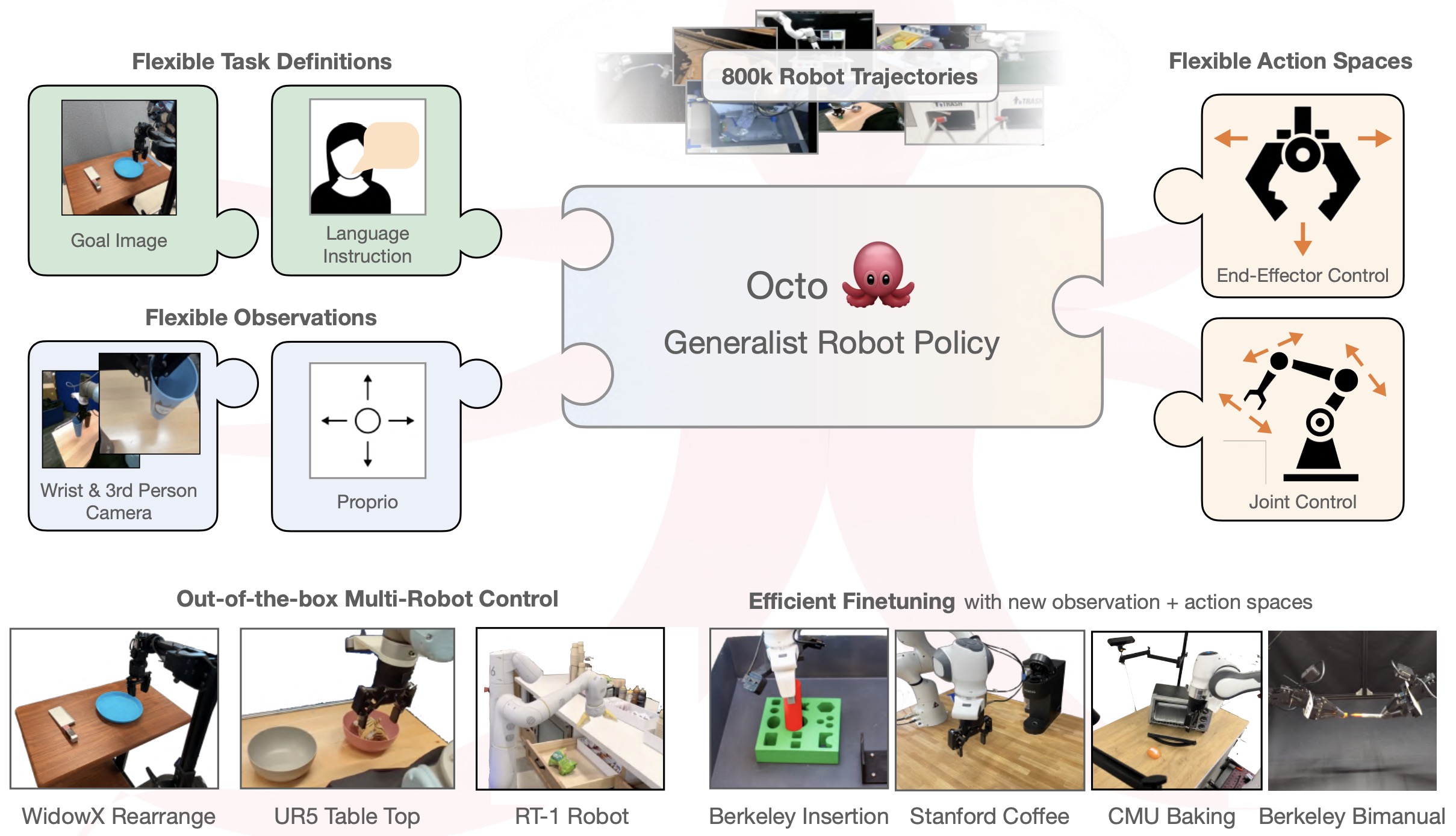
The following figure (source) shows the Octo model architecture with task and observation tokenization, transformer readout tokens, and adaptable action heads.

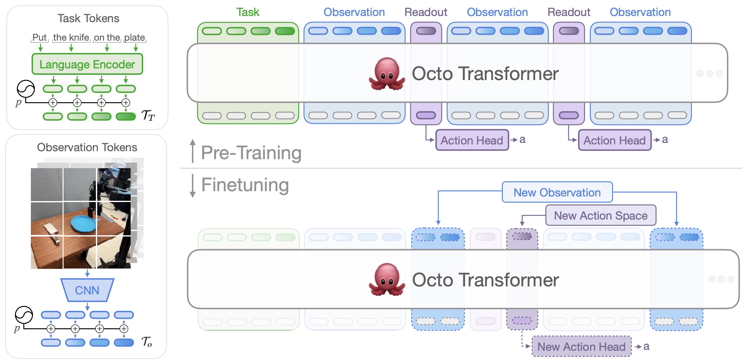
Octo is a transformer-based diffusion policy pretrained on approximately 800,000 trajectories from Open X-Embodiment. Unlike OpenVLA, Octo is designed primarily as a flexible robot policy rather than as a large internet-pretrained VLM converted into a policy. Its inputs can include images, proprioception, language, and goal images.
The Octo project page describes two released model sizes, Octo-Small at 27M parameters and Octo-Base at 93M parameters, with a design explicitly intended to support new sensors, task specifications, and action spaces during fine-tuning. In practice, the representation must preserve the task-relevant geometry, state, and uncertainty needed by downstream reasoning and control rather than only semantic appearance.

Open and Generalist Policies

This section connects octo’s readout architecture with flexible observation spaces. The discussion develops the relevant methods, implementation details, and practical tradeoffs.

Octo’s Readout Architecture

Octo’s readout design treats action prediction as a configurable interface over a shared transformer representation, which makes heterogeneous robot data easier to absorb without forcing every embodiment into an identical native action space.
Octo’s Readout Architecture changes how the policy represents and executes motion, so the chosen temporal horizon and action parameterization must remain compatible with controller rate, embodiment limits, and opportunities for feedback correction.
Octo uses learned readout tokens to extract policy information from the transformer. Let $T_O$ represent observation tokens, $T_G$ task tokens, and $T_R$ learned readout tokens.
The transformer computes:
\[H = \operatorname{Transformer} ( T_O,T_G,T_R )\]
The readout representation $h_R$ is passed to a lightweight action head:
\[a \sim f_{\mathrm{action}}(h_R)\]
In Octo’s default configuration, the action head implements a diffusion objective. This is the point where learned predictions meet coordinate frames, control rates, actuator limits, and the closed-loop dynamics of the physical system.
This creates the separation:
\[\text{shared transformer} \rightarrow \text{readout representation} \rightarrow \text{replaceable output head}\]

Flexible Observation Spaces

A foundation policy benefits from observation interfaces that can absorb different camera layouts, proprioceptive channels, and task inputs without retraining the entire backbone for each sensor configuration.
Flexible Observation Spaces should be evaluated through the behavior it produces after integration, because component-level metrics can miss timing, state-distribution, and control-interface failures that only appear in closed-loop execution.
Robot platforms differ not only in actions but also in sensors. In practice, the representation must preserve the task-relevant geometry, state, and uncertainty needed by downstream reasoning and control rather than only semantic appearance.
A modular token interface can represent:
\[\mathcal{T} = \{ T_{\mathrm{vision}}, T_{\mathrm{state}}, T_{\mathrm{force}}, T_{\mathrm{language}}, T_{\mathrm{goal}}, \ldots \}\]
The transformer can operate on whichever token blocks are available, making modularity increasingly important as Physical AI expands from standardized robot arms toward humanoids and heterogeneous autonomous machines. In practice, the representation must preserve the task-relevant geometry, state, and uncertainty needed by downstream reasoning and control rather than only semantic appearance.

Two Paths to Generalist Robot Policies

Two Paths to Generalist Robot Policies should be analyzed along separate axes such as task, object, scene, language, dynamics, and embodiment because success on one axis does not imply broad physical generalization.
Two Paths to Generalist Robot Policies should distinguish broadly reusable semantic and perceptual representations from robot-specific calibration in kinematics, dynamics, sensing, action ranges, and recovery behavior.
OpenVLA and Octo illustrate two complementary approaches:
\[\boxed{ \text{internet-pretrained semantic model} \rightarrow \text{robot action model} }\]
- and:
  \[\boxed{ \text{large heterogeneous robot dataset} \rightarrow \text{flexible robot foundation policy} }\]
Modern systems increasingly combine both:
\[\boxed{ \text{internet-scale multimodal knowledge} + \text{cross-embodiment robot data} + \text{continuous generative action modeling} }\]

$\pi_0$

$\pi_0$ treats robot control as a foundation-model problem in which multimodal understanding and action generation are trained together, with the action pathway responsible for translating high-level task context into continuous behavior.
For $\pi_0$, the practical question is whether multimodal pretraining and continuous action generation remain aligned once the policy is deployed on a particular robot with its own timing and action conventions.
$\pi_0$: A Vision-Language-Action Flow Model for General Robot Control by Black et al. (2024) introduces a VLA architecture built on a pretrained VLM combined with a flow-matching action expert.
The following figure (source) shows the $\pi_0$ generalist policy, which augments a pretrained VLM with a flow-matching action expert for cross-embodiment dexterous control using a diverse cross-embodiment dataset with a variety of dexterous manipulation tasks. The model is adapted to robot control by adding a separate action expert that produces continuous actions via flow matching, enabling precise and fluent manipulation skills. The model can then be used directly to perform tasks based on a prompt, or fine-tuned on high-quality data to enable complex multi-stage tasks, such as folding multiple articles of laundry or assembling a box.

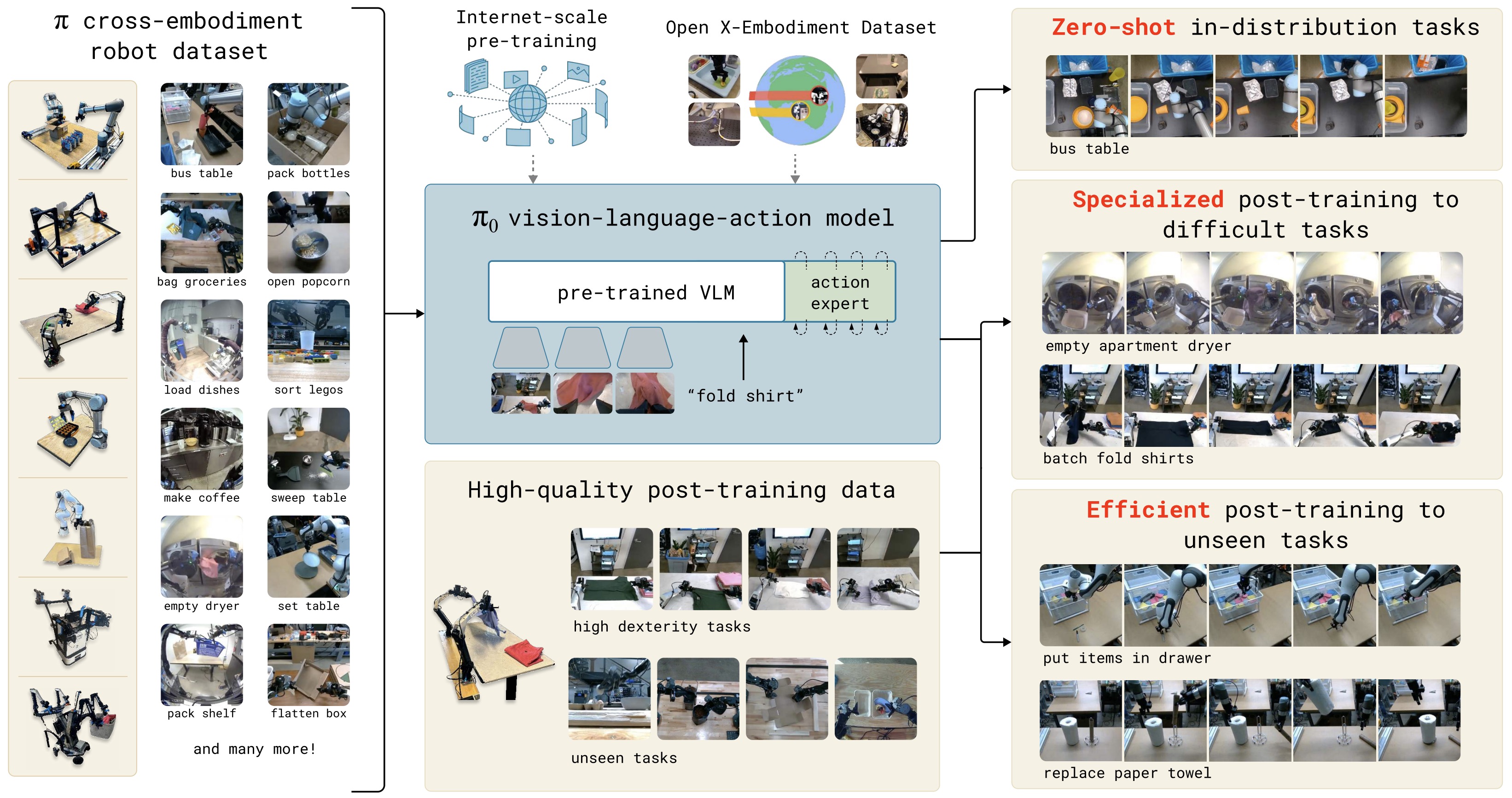
The architecture can be conceptualized as:
\[\boxed{ \text{VLM} + \text{Action Expert} }\]
- rather than treating actions as ordinary language tokens.
The VLM processes visual observations and language:
\[h_{\mathrm{semantic}} = f_{\mathrm{VLM}}(I,l)\]
- while the action expert predicts a continuous vector field:
  \[v_\theta( A^\tau, \tau \mid h_{\mathrm{semantic}}, s )\]
Starting from noise $A^0\sim\mathcal{N}(0,I)$ the action trajectory is transported toward the learned robot-action distribution through:
\[\frac{dA^\tau}{d\tau} = v_\theta( A^\tau, \tau \mid h_{\mathrm{semantic}}, s )\]

The Action Expert

The Action Expert couples model quality to the timing behavior of the deployed system. Observation age, inference duration, action-horizon length, controller frequency, and active compute all affect whether a nominally accurate prediction is still valid when it reaches the actuators.
The Action Expert changes how the policy represents and executes motion, so the chosen temporal horizon and action parameterization must remain compatible with controller rate, embodiment limits, and opportunities for feedback correction.
Instead of requiring the VLM to directly model actions using its text vocabulary, the VLM produces representations consumed by a dedicated motor model:
\[h=f_{\mathrm{VLM}}(I,l)\] \[A=f_{\mathrm{expert}}(h,s,\epsilon)\]
The action expert can operate at a different dimensionality, precision, architecture, and inference cadence from the semantic backbone. For embodied use, that semantic interpretation must remain tied to the current scene, the robot state, and the actions that are actually feasible for the embodiment.
This makes it possible to use a large semantic model for understanding and a specialized generative model for motor control. For embodied use, that semantic interpretation must remain tied to the current scene, the robot state, and the actions that are actually feasible for the embodiment.

Isaac 0.5: Unified Perception, Reasoning, and Control

Isaac 0.5: Unified Perception, Reasoning, and Control integrates perception with downstream reasoning and control so visual representations are trained for the decisions the robot must make rather than for recognition in isolation.
Isaac 0.5: Percepts Scale Control by Perceptron Team et al. (2026) introduces a 36B-parameter open-weight embodied foundation model that unifies video perception, spatial grounding, embodied visual reasoning, and robot control in one sparse backbone. Rather than attaching a policy head to a frozen perceptual encoder, Isaac 0.5 co-trains perception, semantic future prediction, discrete action generation, and continuous control through a shared representation, allowing structure learned from large-scale action-free video to directly influence the context used for control. The accompanying Introducing Isaac 0.5 release describes the model as a single interface over images, video, language, robot state, previous actions, grounding outputs, task progress, and robot actions.
The design can be summarized as a shared embodied representation with several output interfaces:
\[\left( I_{\leq t}, l, s_{\leq t}, a_{<t} \right) \xrightarrow{f_\theta} h_t \rightarrow \left\{ \begin{array}{l} \text{text and grounding}\\ \text{embodied reasoning}\\ \text{FAST action tokens}\\ \text{continuous Flow actions} \end{array} \right\}\]
This differs from architectures in which perception is learned first and then frozen before policy learning. In Isaac 0.5, semantic objectives, autoregressive action supervision, and continuous control all update or condition on the same backbone, so the model is explicitly designed to transfer visual-temporal structure into action prediction. FAST: Efficient Action Tokenization for Vision-Language-Action Models by Pertsch et al. (2025) provides the compression-based action tokenizer used for Isaac 0.5’s discrete action route, while Flow Matching for Generative Modeling by Lipman et al. (2023) provides the continuous generative modeling principle used by its Flow route.

Shared Sparse Backbone and Null-Expert Routing

Isaac 0.5 uses a Qwen-family multimodal architecture with a 2,048-wide trunk of 40 sparse decoder blocks, comprising 30 GDN linear-attention blocks and 10 full-attention blocks. Each block contains 256 routed MLP experts, an always-on shared expert, and a learned null route that allows the number of executed routed experts to vary token by token. Improving MoE Compute Efficiency by Composing Weight and Data Sparsity by Kilian et al. (2026) develops the null-expert mechanism that enables causal token-choice Mixture-of-Experts models to skip routed computation for tokens that do not need the full expert budget.
Standard top-$k$ MoE routing spends a fixed number of expert evaluations on every token. Isaac 0.5 instead exposes eight routing slots but permits any subset of them to become no-op null routes. If $j$ real-expert scores exceed the learned null score, the number of executed and skipped routes is:
\[k_{\mathrm{real}} = \min(8,j)\] \[k_{\mathrm{null}} = 8-k_{\mathrm{real}}\]
- so a token can execute between zero and eight routed experts while retaining access to the full 256-expert library. At the paper’s 50% null reference point, four of eight routes are real and approximately 2.5B of the model’s 36B parameters are active per token; the reported routed active-parameter range is approximately 0.1B to 3B as the number of real routes varies.
Token-adaptive computation is particularly relevant to embodied multimodal sequences because text, image patches, robot state, and action tokens need not require the same amount of processing. The sparse backbone can therefore allocate more routed computation to information-rich regions while allowing less informative tokens to pass primarily through the residual and shared-expert paths.
The following figure (source) shows token-adaptive null routing and the continuous-control DiT: every backbone layer uses the same sparse feed-forward block, null routes skip routed MLP computation, and the continuous-control DiT cross-attends to masked pre-action backbone context before predicting the velocity field whose integration yields a continuous action chunk.

Semantic Future-Percept Prediction

A central contribution of Isaac 0.5 is a self-supervised semantic world-modeling objective over action-free video. Instead of reconstructing future pixels, the model predicts a future percept: a task-relevant visible state or change such as an object state, spatial relation, affordance, task phase, visible contact transition, or likely near-future task state. Isaac 0.5: Percepts Scale Control by Perceptron Team et al. (2026) places this target between low-level video prediction and direct action prediction, with the goal of retaining semantic information that is useful for downstream control.
Given observation history $o_{\leq t}$ and a future percept target $z_{t+\Delta}$, the disclosed boundary of the objective is:
\[\mathcal{L}_{\mathrm{sem}} = \mathbb{E}_{(o_{\leq t},z_{t+\Delta})} \left[ \ell \left( g_\theta(o_{\leq t}), z_{t+\Delta} \right) \right]\]
- where $g_\theta$ is the semantic predictor and $\Delta>0$ is the prediction offset. The construction of $z_{t+\Delta}$ and the implementation of $\ell$ are not disclosed; importantly, the targets are generated automatically from future video observations without human action labels.
This formulation creates a third route between pixel-level world modeling and action-only policies:
\[\boxed{ \text{future pixels} \quad\longleftrightarrow\quad \text{future percepts} \quad\longleftrightarrow\quad \text{future actions} }\]
The distinction is useful for Physical AI because a control-relevant representation need not predict every visual detail. A semantic percept objective can instead emphasize state changes and task progress that matter for action while still exploiting video that contains no robot proprioception or control labels.

Dual Discrete and Continuous Action Interfaces

Isaac 0.5 exposes both autoregressive discrete control and continuous generative control from the same backbone. The discrete route converts a normalized action chunk $a$ into a FAST token sequence $q=\operatorname{FAST}(a)$ and trains those tokens under the same autoregressive next-token objective used by the model’s other discrete outputs:
\[\mathcal{L}_{\mathrm{FAST}} = -\sum_j \log p_\theta \left( q_j \mid c,q_{<j} \right)\]
- where $c$ is the shared-backbone context. FAST: Efficient Action Tokenization for Vision-Language-Action Models by Pertsch et al. (2025) compresses temporally structured continuous actions in frequency space so autoregressive VLAs can model dexterous, high-frequency trajectories more effectively than per-dimension binning.
The continuous route uses a dedicated 36-block, width-768 Diffusion Transformer conditioned on the shared backbone through cross-attention. For each action chunk, Isaac 0.5 samples $S=4$ independent noise levels using:
\[\epsilon_s \sim \mathcal{N}(0,I)\] \[z_s \sim \operatorname{Beta}(1.5,1)\] \[\tau_s = 0.001+0.999z_s\] \[x_s = (1-\tau_s)a+\tau_s\epsilon_s\]
- and uses Flow time $t_s=1-\tau_s$. The straight conditional path has target velocity $a-\epsilon_s$, yielding the masked action-chunk objective:
\[\mathcal{L}_{\mathrm{Flow}} = \frac{1}{S} \sum_{s=1}^{S} \frac{ \left\| M \odot \left[ \hat v_\theta(x_s,t_s;c) - (a-\epsilon_s) \right] \right\|_2^2 }{ \|M\|_1 }\]
- where $M$ masks padded time steps and unused action dimensions. This is closely related to the flow-matching action generation used by $\pi_0$: A Vision-Language-Action Flow Model for General Robot Control by Black et al. (2024), but Isaac 0.5 retains both the FAST autoregressive route and the continuous Flow route within one shared embodied model.
The resulting joint objective combines next-token prediction, semantic future-percept prediction, continuous Flow control, and sparse-routing regularization:
\[\mathcal{L}_{\mathrm{train}} = \mathcal{L}_{\mathrm{NTP}} + \mathcal{L}_{\mathrm{sem}} + 10^{-4}\mathcal{L}^{\mathrm{LM}}_{z} + \mathcal{L}_{\mathrm{Flow}} + 0.02\mathcal{L}_{\mathrm{MoE\mbox{-}LB} } + 10^{-3}\mathcal{L}^{\mathrm{router}}_{z}\]
The important coupling is that the Flow objective is not isolated behind a detached frozen representation: the control loss updates the Flow path and shared backbone, while semantic, autoregressive, and router objectives also update the backbone. Consequently, the representation used by the action generator is shaped jointly by video understanding, embodied reasoning, and control supervision.

Typed Multimodal Training with mHarmony

Training one representation across heterogeneous embodied sources requires preserving modality- and embodiment-specific semantics rather than flattening every input into an undifferentiated token stream. Isaac 0.5: Percepts Scale Control by Perceptron Team et al. (2026) uses mHarmony, a typed multimodal compiler that validates source schemas, resolves embodiment-specific state and coordinate conventions, aligns clocks, and emits packed TensorStream events containing text, vision, time, robot state, and FAST tokens.
Continuous Flow targets remain keyed outside the discrete token stream but are aligned to the same observations, while causal action history can re-enter the context as typed history. This preserves a crucial distinction: missing robot actions in ordinary video are not treated as negative action labels, and continuous control targets are not forced into a representation intended for language tokens.
The following figure (source) shows the heterogeneous-data path into Isaac 0.5: mHarmony validates and lowers source schemas into typed TensorStream events before packing, after which the shared visual encoder and sparse backbone support perception, embodied reasoning, FAST discrete control, and a Flow/DiT continuous-control interface.

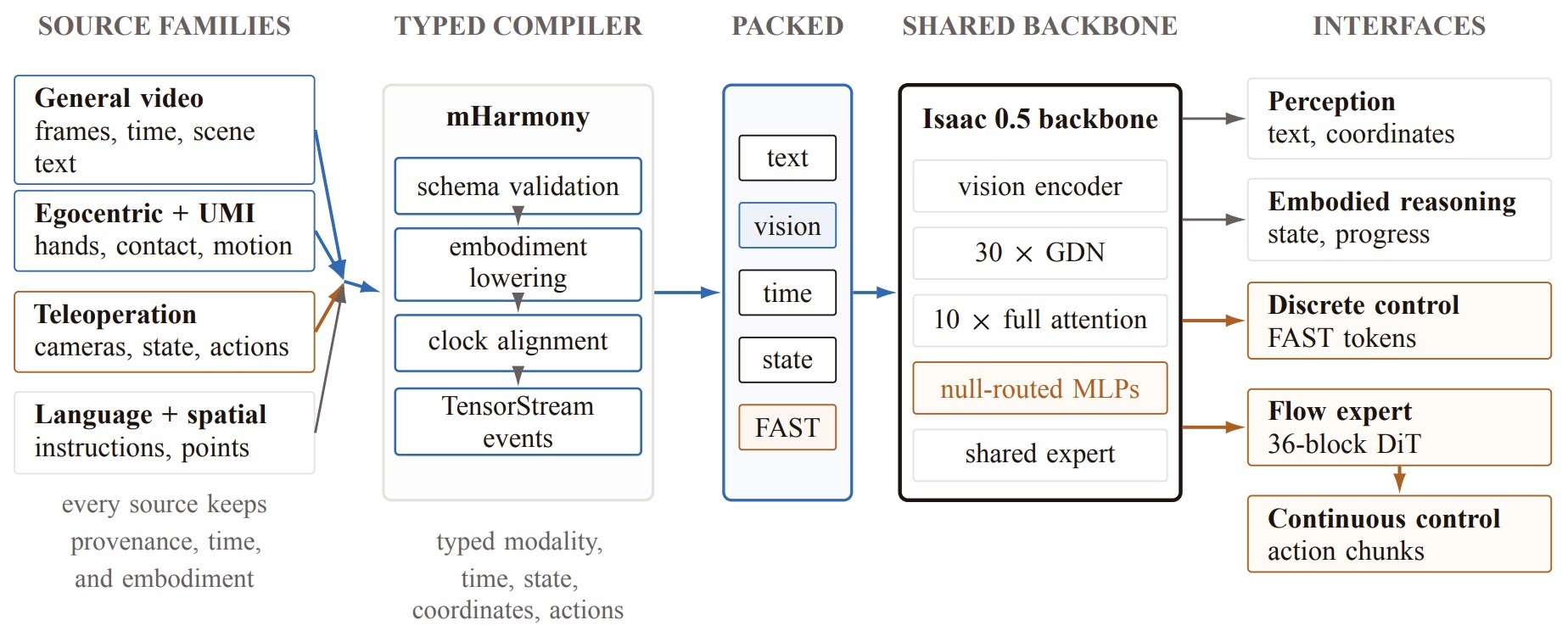
Scaling Action-Free Video Against Teleoperation

Isaac 0.5 directly studies whether broad action-free video can reduce the amount of expensive teleoperated robot data required to reach a fixed control-quality target. The training inventory spans one million hours of general video, 375,000 hours of egocentric video, 375,000 hours of UMI-style handheld-gripper video, approximately 100,000 hours of robotics-oriented experience, and 3T multimodal tokens, with robot interfaces covering more than 35 embodiment configurations. Universal Manipulation Interface: In-The-Wild Robot Teaching Without In-The-Wild Robots by Chi et al. (2024) motivates the UMI-style intermediate regime by collecting manipulation demonstrations through portable handheld grippers rather than requiring a deployed robot for every trajectory.
The data sources provide complementary forms of supervision. General video supplies broad object, activity, and environment coverage; egocentric video concentrates on hands, contact, and task progress; UMI provides gripper motion and timing closer to robot manipulation; teleoperation supplies the strongest embodiment-specific state-action grounding. Introducing Isaac 0.5 describes these sources as a continuum from inexpensive visual experience to costly but precise robot control supervision.
To isolate the interaction between video and robot action data, the scaling experiment holds the relative general-video:egocentric:UMI composition at $80:30:30$ while varying total video exposure and teleoperation hours. At the reported offline action-loss threshold $\tau=2.50$, increasing general video from $1{,}000$ to $1{,}000{,}000$ hours moves the interpolated within-grid teleoperation crossing from $5{,}884$ hours to $28$ hours:
\[\frac{5{,}884}{28} \approx 210.3\]
This should not be interpreted as a universal constant exchange rate between video and robot data. Isaac 0.5: Percepts Scale Control by Perceptron Team et al. (2026) reports that the adjacent measured teleoperation rungs bound the headline ratio at approximately $83\times$ to $300\times$, and the benefit of additional video is strongly conditioned on sufficient action grounding. With only one hour of teleoperation, a $10\times$ increase in video changes loss by only about $-0.006$; from roughly 100 teleoperation hours onward, the empirical change stabilizes near $-0.21$ loss per $10\times$ increase in video.
The following figure (source) shows the measured video-teleoperation scaling grid: fixed-loss contours reveal the reported 210.3× reduction in teleoperation at loss 2.50, empirical slopes show that video becomes more useful once sufficient action grounding is present, and non-perceptive comparison runs remain above loss 2.75 across the measured video budgets.

Cross-Embodiment Control and Adaptation

The released checkpoint contains robot-specific observation, action, normalization, timing, and safety configurations for more than 35 embodiment interfaces represented during training. A shared policy can therefore retain common visual and task representations while resolving control semantics through an embodiment configuration rather than assuming that heterogeneous robots expose interchangeable action spaces.
The technical report demonstrates this interface by executing the same requested cup-stacking task on YAM and SO-101 hardware with one checkpoint and changing the embodiment string in the configuration prompt. This does not imply zero-shot transfer to arbitrary unseen kinematics; rather, it demonstrates that multiple trained embodiments can share one backbone while preserving platform-specific control contracts.
The following figure (source) shows one Isaac 0.5 checkpoint executing the same cup-stacking task on YAM and SO-101 embodiments, with paired rollouts aligned by task phase from initial reach through intermediate placement to the completed stack.

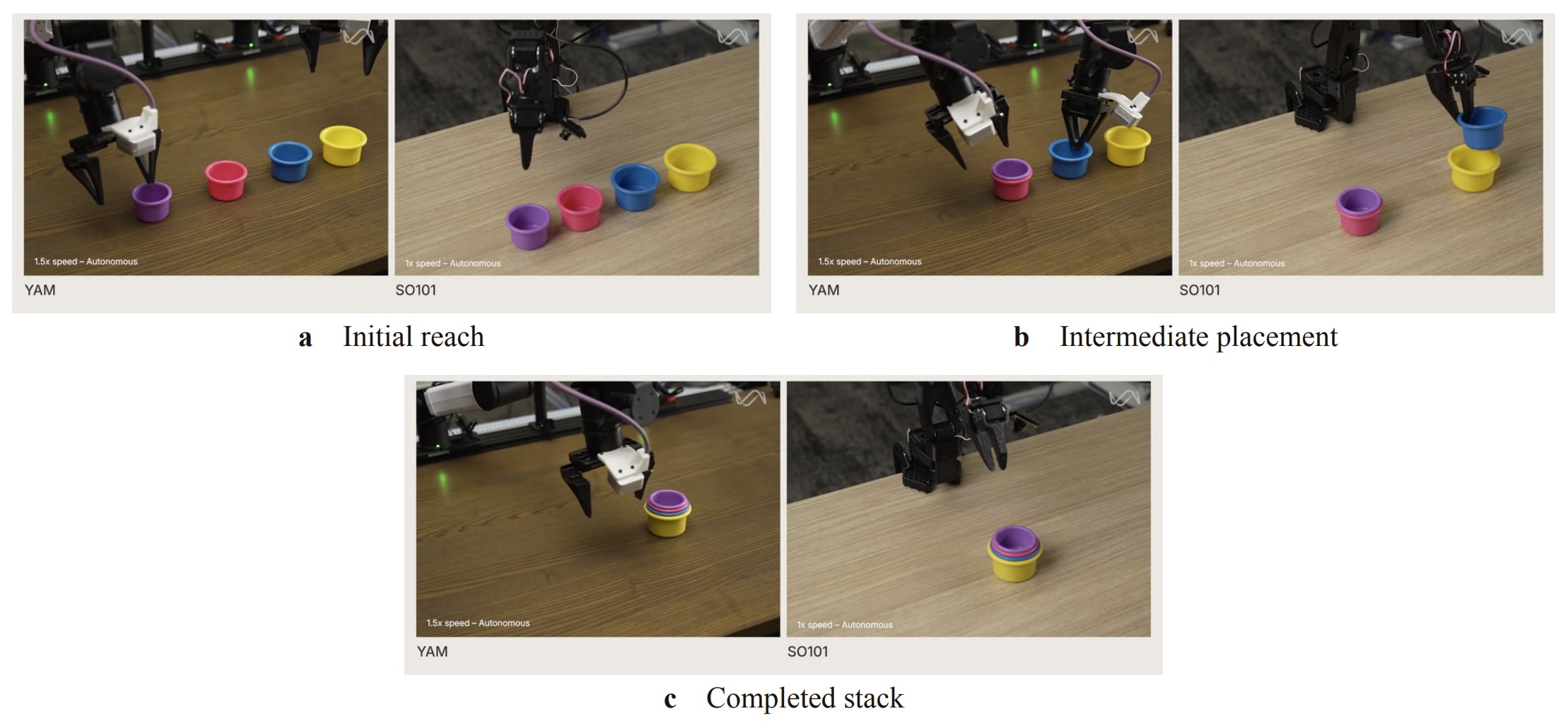
Implications for Generalist Physical AI

Isaac 0.5 extends the generalist-policy design space along three axes. First, it treats action-free video as a first-class source of control-relevant representation learning rather than merely a source for initializing a visual encoder. Second, it unifies semantic perception, embodied reasoning, and multiple action-generation interfaces inside one trainable backbone. Third, null-expert routing introduces token-adaptive sparse compute, allowing model capacity to scale without requiring every multimodal token to execute the same routed workload.
The model therefore combines ideas that appear separately elsewhere in the Physical AI stack:
\[\boxed{ \text{video-scale representation learning} + \text{semantic future prediction} + \\ \text{cross-embodiment action grounding} + \text{FAST and Flow control} + \\ \text{adaptive sparse compute} }\]
This architecture also sharpens the distinction between a general-purpose multimodal backbone and a deployment-ready robot controller. The shared model can transfer visual-temporal and semantic structure broadly, but execution still depends on embodiment-specific state definitions, action normalization, timing, safety limits, and adaptation. Generality therefore comes from sharing representations and training signals while retaining explicit physical interfaces rather than erasing embodiment differences.

Suggested Narrative Edits Elsewhere in the Primer

The Physical AI Data Engine — Human Video, UMI, and Data Mixtures: add Isaac 0.5 as a quantitative example of the hypothesis that action-free video can reduce dependence on teleoperated robot demonstrations when sufficient action grounding is present. The key narrative addition is that general video, egocentric video, UMI-style handheld-gripper data, and teleoperation should be treated as complementary supervision sources rather than interchangeable samples, with the measured benefit of video depending strongly on the amount of robot action data.
Training and Post-Training — From Foundation Model to Physical Policy: add Isaac 0.5 as a counterpoint to pipelines that pretrain a visual-language encoder and attach or fine-tune a downstream action head. Its semantic, autoregressive, continuous-control, and router objectives co-train the shared backbone, illustrating a training regime in which perception, reasoning, and control remain coupled throughout pretraining.
World Models for Physical AI — World Models and Policies: add semantic future-percept prediction as an intermediate world-model target between future-pixel generation and direct action prediction. Isaac 0.5 is useful here because its percept objective predicts task-relevant future states and changes from action-free video while deliberately avoiding full pixel reconstruction.
Vision-Language-Action Models — Tokenized Versus Continuous Actions: extend the tokenized-versus-continuous comparison with Isaac 0.5’s dual interface. The same shared backbone supports autoregressive FAST tokens and a continuous Flow/DiT action expert, demonstrating that these action parameterizations need not be mutually exclusive at the foundation-model level.
Engineering a Physical AI System — Inference and Compute: add null-expert routing as an example of adaptive inference for heterogeneous multimodal workloads. Isaac 0.5 permits each token to execute between zero and eight routed experts, separating total model capacity from active routed compute while retaining an always-on shared path.
Open Problems and Research Directions — Scaling Robot Data: add the Isaac 0.5 video-teleoperation experiment as evidence that the marginal value of passive video depends on action grounding. The result motivates scaling laws over data composition rather than treating total hours or total tokens as sufficient predictors of embodied capability.

Flow-Based VLAs

This section connects flow matching for continuous control with cross-embodiment training in $\pi_0$. The discussion develops the relevant methods, implementation details, and practical tradeoffs.

Flow Matching for Continuous Control

Flow Matching for Continuous Control learns a continuous transport field from a simple base distribution to robot action trajectories, providing a multimodal action decoder that can often be sampled with fewer integration steps than diffusion.
Flow Matching for Continuous Control changes how the policy represents and executes motion, so the chosen temporal horizon and action parameterization must remain compatible with controller rate, embodiment limits, and opportunities for feedback correction.
For expert action chunk $A_1$ and noise $A_0$, define:
\[A_\tau=(1-\tau)A_0+\tau A_1\]
The desired vector field is:
\[u_\tau=A_1-A_0\]
The action expert learns $v_\theta(A_\tau,\tau,c)$ using:
\[\mathcal{L}_{\mathrm{flow}} = \mathbb{E} \left[ \| v_\theta(A_\tau,\tau,c)-u_\tau \|_2^2 \right]\]
- where:
  \[c=\{I,l,s\}\]
At inference time, numerical integration generates a coherent continuous action chunk. This is the point where learned predictions meet coordinate frames, control rates, actuator limits, and the closed-loop dynamics of the physical system.

Cross-Embodiment Training in $\pi_0$

Cross-Embodiment Training in $\pi_0$ distinguishes reusable semantic and perceptual structure from the robot-specific kinematics, dynamics, sensing, and action conventions required for successful execution.
Cross-Embodiment Training in pi_0 must be analyzed as part of the timed execution path from observation to actuation, because stale state, wrong frames, or delayed commands can invalidate an otherwise accurate prediction.
A generalist VLA must train across heterogeneous robots:
\[\mathcal{D} = \mathcal{D}_{e_1} \cup \mathcal{D}_{e_2} \cup \cdots \cup \mathcal{D}_{e_N}\]
$\pi_0$: A Vision-Language-Action Flow Model for General Robot Control by Black et al. (2024) trains across diverse dexterous platforms including single-arm, dual-arm, and mobile-manipulator systems.
Training requires normalized or embodiment-aware action representations so shared parameters can learn reusable structure without confusing incompatible control semantics. For embodied use, that semantic interpretation must remain tied to the current scene, the robot state, and the actions that are actually feasible for the embodiment.

$\pi_{0.5}$ and Open-World Generalization

$\pi_{0.5}$ by Physical Intelligence et al. (2025) extends the VLA objective toward open-world manipulation by combining web-scale semantic data with robot experience so that linguistic and visual generalization can support long-horizon physical tasks.
$pi_{0.5}$ and Open-World Generalization should report the task distribution, trial protocol, failure criteria, and interaction budget explicitly so improvements can be attributed to capability rather than easier scenarios or hidden assistance.
$\pi_{0.5}$: a Vision-Language-Action Model with Open-World Generalization by Black et al. (2025) extends the VLA paradigm toward long-horizon operation in previously unseen environments.
The training distribution combines heterogeneous sources:
\[\mathcal{D} = \mathcal{D}_{\mathrm{robot}} + \mathcal{D}_{\mathrm{web}} + \mathcal{D}_{\mathrm{semantic}} + \mathcal{D}_{\mathrm{perception}}\]
The model can consequently learn both low-level action mappings and higher-level semantic predictions, moving from pure motor generalization toward open-world physical reasoning. For embodied use, that semantic interpretation must remain tied to the current scene, the robot state, and the actions that are actually feasible for the embodiment.

Hierarchical Prediction in VLAs

Hierarchical Prediction in VLAs separates decisions that benefit from slower semantic reasoning from those that require fast, stable control. The boundary between these levels is operationally important: high-level modules should expose goals or constraints that remain meaningful long enough for the low-level controller to execute them.
Hierarchical Prediction in VLAs should optimize for decision-relevant prediction: contact, geometry, timing, and task progress matter when they change which action is preferred, whereas visually conspicuous errors may be harmless if they do not affect control.
Long-horizon tasks benefit from separating semantic subgoals from low-level actions:
\[l \xrightarrow{\text{semantic policy}} g_k \xrightarrow{\text{action policy}} A_k\]
This reduces the effective reasoning horizon and allows high-level planning to operate at a slower cadence than motor control. For embodied use, that semantic interpretation must remain tied to the current scene, the robot state, and the actions that are actually feasible for the embodiment.

Tokenized Versus Continuous Actions

Tokenized Versus Continuous Actions determines how continuous control trajectories are represented inside a sequence model. Discretization can reuse language-model machinery, but token granularity, sequence length, temporal compression, and reconstruction error directly affect both optimization and the fidelity of executed motion.
Tokenized Versus Continuous Actions changes how the policy represents and executes motion, so the chosen temporal horizon and action parameterization must remain compatible with controller rate, embodiment limits, and opportunities for feedback correction.
Modern VLA design can be organized around a central choice. This is the point where learned predictions meet coordinate frames, control rates, actuator limits, and the closed-loop dynamics of the physical system.

Tokenized actions

Examples include RT-2 and the original OpenVLA:
\[p(q(a)\mid I,l)\]
Advantages include architectural simplicity and reuse of language-model training infrastructure. Limitations include quantization, sequential decoding latency, and a mismatch between categorical tokens and continuous control geometry.

Continuous regression

OpenVLA-OFT demonstrates direct regression:
\[\hat A=f_\theta(I,l,s)\]
- with an objective such as:
  \[\mathcal{L}=\|A-\hat A\|_1\]
This provides fast parallel decoding but can struggle with strongly multimodal action distributions. This is the point where learned predictions meet coordinate frames, control rates, actuator limits, and the closed-loop dynamics of the physical system.

Diffusion

Octo and Diffusion Policy-style architectures model $p(A\mid I,l,s)$ through iterative denoising. This is the point where learned predictions meet coordinate frames, control rates, actuator limits, and the closed-loop dynamics of the physical system.

Flow matching

$\pi_0$ uses $\frac{dA}{d\tau} = v_\theta(A,\tau,c)$. For control, the benefit is the ability to represent multimodal temporally coherent action distributions, while inference cost and replanning cadence remain deployment constraints.
The appropriate choice depends on control frequency, task multimodality, model size, inference hardware, embodiment, and required precision. This is the point where learned predictions meet coordinate frames, control rates, actuator limits, and the closed-loop dynamics of the physical system.
These action representations can also be contrasted with the emerging WAM formulation. Tokenized, regression, diffusion, and flow-matching VLAs primarily parameterize an action distribution, whereas FLUX 3 Action jointly predicts a future visual trajectory and the action chunk associated with that trajectory:
\[\underbrace{p_\theta\left(a_{t:t+H}\mid o_{\leq t},s_{\leq t},g\right)}_{\text{VLA}} \quad\longrightarrow\quad \underbrace{p_\theta\left(o_{t+1:t+H},a_{t:t+H}\mid o_{\leq t},s_{\leq t},g\right)}_{\text{WAM}}\]
The distinction is architectural rather than merely a choice of action decoder. World Action Models are Zero-shot Policies by Ye et al. (2026) shows how a video-pretrained generative model can become a closed-loop policy, while mimic-video: Video-Action Models for Generalizable Robot Control Beyond VLAs by Pai et al. (2025) instead retains a pretrained video representation and attaches an action decoder. These approaches place video prediction at different points on the path from perception to control.

The VLA Training Mixture

VLA performance depends on the composition of the training mixture because web data, robot trajectories, synthetic examples, and embodiment-specific demonstrations contribute different kinds of supervision: semantics, task diversity, physical grounding, and control calibration.
The VLA Training Mixture should connect semantic intent to the current physical state and available actions, with execution feedback used to verify that the chosen interpretation actually produced the intended effect.
A foundation VLA may draw from several data sources:
\[\mathcal{D}_{\mathrm{total}} = \mathcal{D}_{\mathrm{VLM}} \cup \mathcal{D}_{\mathrm{robot}} \cup \mathcal{D}_{\mathrm{human}} \cup \mathcal{D}_{\mathrm{synthetic}}\]
Vision-language data provides semantic knowledge, robot trajectories provide action grounding, human video provides physical interaction priors, and simulation and synthetic data provide scale and coverage. In practice, the representation must preserve the task-relevant geometry, state, and uncertainty needed by downstream reasoning and control rather than only semantic appearance.
The mixture weights become an important hyperparameter:
\[\mathcal{L} = \lambda_{\mathrm{VLM}} \mathcal{L}_{\mathrm{VLM}} + \lambda_{\mathrm{robot}} \mathcal{L}_{\mathrm{robot}} + \lambda_{\mathrm{aux}} \mathcal{L}_{\mathrm{aux}}\]
VLA training is therefore partly a problem of balancing semantic retention against physical specialization. For embodied use, that semantic interpretation must remain tied to the current scene, the robot state, and the actions that are actually feasible for the embodiment.

Action Representations and Deployment

This section connects normalizing heterogeneous robot data with control frequency and inference latency. The discussion develops the relevant methods, implementation details, and practical tradeoffs.

Normalizing Heterogeneous Robot Data

Normalizing Heterogeneous Robot Data prevents representational mismatches from being mistaken for learning problems. Units, coordinate frames, action conventions, timing, padding, and embodiment metadata must remain explicit so heterogeneous examples describe comparable physical quantities.
Normalizing Heterogeneous Robot Data should be assessed by the new behavioral coverage it contributes, especially rare states, recovery situations, and observation-action combinations that are missing from the current training distribution.
Cross-embodiment datasets rarely share action conventions. This is the point where learned predictions meet coordinate frames, control rates, actuator limits, and the closed-loop dynamics of the physical system.
Actions can be normalized as
\[\tilde a^{(e)} = N_e(a^{(e)})\]
- where $N_e$ is an embodiment- or dataset-specific normalization function.
The policy learns:
\[\tilde a=\pi_\theta(o,l,e)\]
- and deployment applies:
  \[a^{(e)}=N_e^{-1}(\tilde a)\]
Data standardization is therefore part of the model architecture in practice, not merely preprocessing. What matters is not only the number of examples but also their coverage of tasks, embodiments, recovery states, and observation-action alignments that the deployed policy will encounter.

Control Frequency and Inference Latency

Control Frequency and Inference Latency couples model quality to the timing behavior of the deployed system. Observation age, inference duration, action-horizon length, controller frequency, and active compute all affect whether a nominally accurate prediction is still valid when it reaches the actuators.
Control Frequency and Inference Latency determines whether observations are still current when the corresponding action reaches the controller, making end-to-end delay and overlap between sensing, inference, and actuation part of policy correctness.
A VLA deployed on a robot is a real-time system. This is the point where learned predictions meet coordinate frames, control rates, actuator limits, and the closed-loop dynamics of the physical system.
For target control frequency $f_c$, the inference budget is approximately:
\[T_{\max}=\frac{1}{f_c}\]
The latency budget includes:
\[T_{\mathrm{camera}} + T_{\mathrm{preprocess}} + T_{\mathrm{vision}} + T_{\mathrm{policy}} + T_{\mathrm{decode}} + T_{\mathrm{communication}}\]
If $T_{\mathrm{total}}>T_{\max}$, the policy cannot maintain the desired control rate. This is the point where learned predictions meet coordinate frames, control rates, actuator limits, and the closed-loop dynamics of the physical system.
Autoregressive generation, diffusion sampling, numerical flow integration, image resolution, context length, and model size therefore directly affect physical control performance. In practice, the representation must preserve the task-relevant geometry, state, and uncertainty needed by downstream reasoning and control rather than only semantic appearance.

Asynchronous Inference

Asynchronous Inference couples model quality to the timing behavior of the deployed system. Observation age, inference duration, action-horizon length, controller frequency, and active compute all affect whether a nominally accurate prediction is still valid when it reaches the actuators.
Asynchronous Inference determines whether observations are still current when the corresponding action reaches the controller, making end-to-end delay and overlap between sensing, inference, and actuation part of policy correctness.
One solution is to overlap policy inference and robot execution. While the robot executes $A_t$, the model can begin computing $A_{t+K}$.
This reduces idle time but introduces stale-observation risk, producing a tradeoff between latency and observation freshness. In practice, the representation must preserve the task-relevant geometry, state, and uncertainty needed by downstream reasoning and control rather than only semantic appearance.

Fine-Tuning Strategy

Fine-Tuning Strategy is where a broad foundation policy is aligned with the target robot, task distribution, and deployment constraints. The adaptation procedure must decide which shared representations should remain stable and which components must change to capture embodiment-specific dynamics, action conventions, and failure modes.
Fine-Tuning Strategy depends on the feedback channel available during adaptation: offline supervision favors conservative updates within known data, whereas interactive feedback can correct new failure states at the cost of additional exploration and safety management.
Adapting a VLA can involve full fine-tuning, frozen-backbone action-head training, or parameter-efficient fine-tuning. This is the point where learned predictions meet coordinate frames, control rates, actuator limits, and the closed-loop dynamics of the physical system.
LoRA introduces low-rank updates:
\[W'=W+BA\]
- where:
  \[\operatorname{rank}(BA)\ll\operatorname{dim}(W)\]
The OpenVLA project reports strong LoRA-based adaptation results. The training stage should therefore be interpreted by the capability it is intended to add: broad representations, embodiment grounding, task adaptation, or closed-loop behavioral improvement.
The appropriate strategy depends on the size of the domain shift:
\[\boxed{ \text{fine-tuning scope} \propto \text{magnitude of distribution shift} }\]

What Makes a VLA Generalist?

A VLA becomes meaningfully generalist when the same policy can preserve competence as tasks, objects, scenes, language, and embodiments vary, rather than merely sharing a backbone across narrowly related datasets.
What Makes a VLA Generalist? should connect semantic intent to the current physical state and available actions, with execution feedback used to verify that the chosen interpretation actually produced the intended effect.
Generalization can occur along several dimensions:
\[G_{\mathrm{VLA}} = G_{\mathrm{semantic}} \times G_{\mathrm{visual}} \times G_{\mathrm{task}} \times G_{\mathrm{motion}} \times G_{\mathrm{environment}} \times G_{\mathrm{embodiment}}\]
A model can perform strongly on one dimension while failing on another. Evaluating VLA generality therefore requires substantially richer benchmarks than measuring success on tasks drawn from the training distribution.

The Emerging VLA Design Pattern

Modern VLA systems increasingly separate broad multimodal reasoning from specialized action generation, allowing semantic representations to scale with foundation-model pretraining while continuous control is handled by token, diffusion, or flow-based action modules.
The Emerging VLA Design Pattern should connect semantic intent to the current physical state and available actions, with execution feedback used to verify that the chosen interpretation actually produced the intended effect.
Across RT-2, OpenVLA, Octo, OpenVLA-OFT, $\pi_0$, and $\pi_{0.5}$, a common architecture is emerging:
\[\boxed{ \begin{array}{c} \text{Images + Language + Robot State}\\ \downarrow\\ \text{Pretrained Visual / Multimodal Representations}\\ \downarrow\\ \text{Shared Transformer Backbone}\\ \downarrow\\ \text{Semantic / Physical Representation}\\ \downarrow\\ \text{Specialized Action Decoder}\\ \downarrow\\ \text{Action Chunk}\\ \downarrow\\ \text{Robot Controller} \end{array} }\]
The major trend is away from treating robot actions as merely another type of language token and toward preserving a powerful pretrained multimodal backbone while introducing action-specific architectures. For embodied use, that semantic interpretation must remain tied to the current scene, the robot state, and the actions that are actually feasible for the embodiment.
This can be summarized as:
\[\boxed{ \text{foundation semantics} + \text{robot experience} + \text{continuous generative control} }\]
The semantic model answers what should happen. The action model determines how the embodiment should make it happen.
This architecture forms the basis for increasingly capable humanoid foundation models. The next section will examine NVIDIA Isaac GR00T and the broader humanoid Physical AI stack, including GR00T N1, later GR00T models, dual-system architectures, whole-body and bimanual control, embodiment adaptation, synthetic robot data, GR00T-Dreams, Isaac Sim, Isaac Lab, Newton, and sim-to-real training.

Isaac GR00T and Humanoid Foundation Models

Humanoid foundation models must bridge broad semantic understanding and precise physical control. This chapter follows the GR00T architecture through its data sources, model evolution, training infrastructure, and evaluation.

Humanoid Learning and GR00T Architecture

This section develops why humanoids are a distinct physical ai problem in the context of the broader Physical AI system. It connects the underlying concepts to the implementation details discussed below.

Why Humanoids Are a Distinct Physical AI Problem

Why Humanoids Are a Distinct Physical AI Problem is distinguished by whole-body coordination, contact, balance, and high-dimensional actuation, which couple perception and planning tightly to dynamics and control frequency.
Why Humanoids Are a Distinct Physical AI Problem couples multiple physical constraints such as contact, balance, actuator limits, timing, and whole-body coordination, so local action plausibility is insufficient without trajectory-level execution context.
Humanoid robots occupy an unusual position in Physical AI. Their morphology is designed around environments built for humans, which potentially allows them to use doors, tools, shelves, workstations, vehicles, and other infrastructure without redesigning the environment.
At the same time, humanoid control combines several difficult problems:
\[\text{Humanoid Intelligence} = \text{Perception} + \text{Reasoning} + \text{Manipulation} + \text{Locomotion} + \text{Whole-Body Control}\]
A mobile manipulator may control one arm and a mobile base. A humanoid may need to coordinate two arms, dexterous hands, torso, head, and legs while simultaneously maintaining balance.
The action space can therefore contain dozens of coupled degrees of freedom:
\[a_t = [ a_t^{\mathrm{left\ arm}}, a_t^{\mathrm{right\ arm}}, a_t^{\mathrm{torso}}, a_t^{\mathrm{hands}}, a_t^{\mathrm{legs}} ]\]
The challenge becomes even greater because many useful tasks are long-horizon:
\[\text{navigate} \rightarrow \text{locate object} \rightarrow \text{reach} \rightarrow \text{grasp} \rightarrow \text{manipulate} \rightarrow \text{recover}\]
A general-purpose humanoid therefore needs semantic reasoning at long timescales and precise motor control at short timescales. For embodied use, that semantic interpretation must remain tied to the current scene, the robot state, and the actions that are actually feasible for the embodiment.
NVIDIA’s Isaac GR00T platform is designed around this broader problem, combining robot foundation models, data pipelines, simulation, middleware, accelerated runtime libraries, and deployment infrastructure rather than treating the VLA as an isolated model.

From Project GR00T to GR00T N1

From Project GR00T to GR00T N1 highlights the additional coupling introduced by high-dimensional embodiments. Manipulation quality depends not only on local hand or arm motion but also on coordinated state estimation, balance, reachability, contact, and the timing relationships among multiple controlled body segments.
From Project GR00T to GR00T N1 couples multiple physical constraints such as contact, balance, actuator limits, timing, and whole-body coordination, so local action plausibility is insufficient without trajectory-level execution context.
NVIDIA introduced Project GR00T in 2024 as an initiative to develop general-purpose foundation models for humanoid robots. The design choice determines how much semantic knowledge can be shared across tasks while still preserving the precision and timing required by the robot-specific action interface.
The first major open model from this effort was GR00T N1: An Open Foundation Model for Generalist Humanoid Robots by NVIDIA et al. (2025), a Vision-Language-Action model designed around a dual-system architecture and trained from real robot trajectories, human video, simulation, and synthetic data.
The high-level architecture can be represented as:
\[\boxed{ \text{Vision + Language + Robot State} \rightarrow \text{System 2} \rightarrow \text{System 1} \rightarrow \text{Continuous Actions} }\]
- where the two systems operate at different levels of abstraction.
This separation addresses a fundamental mismatch in embodied intelligence:
\[T_{\mathrm{reasoning}} \gg T_{\mathrm{control}}\]
A robot may need substantial computation to interpret a novel instruction but must continue producing smooth physical actions at a much faster cadence. For embodied use, that semantic interpretation must remain tied to the current scene, the robot state, and the actions that are actually feasible for the embodiment.

The Dual-System Architecture

The Dual-System Architecture separates slower multimodal reasoning from faster continuous action generation, allowing each pathway to operate at the representation and cadence best matched to its role while sharing task context.
The Dual-System Architecture should be evaluated through the behavior it produces after integration, because component-level metrics can miss timing, state-distribution, and control-interface failures that only appear in closed-loop execution.
GR00T N1 explicitly adopts a dual-system design inspired by the distinction between deliberate reasoning and fast intuitive behavior. For embodied use, that semantic interpretation must remain tied to the current scene, the robot state, and the actions that are actually feasible for the embodiment.
GR00T N1: An Open Foundation Model for Generalist Humanoid Robots by NVIDIA et al. (2025) implements System 2 as a vision-language module that interprets visual observations and language instructions, while System 1 is a Diffusion Transformer that converts the resulting representation and robot state into continuous motor actions. Conceptually, $h_t = f_{\mathrm{VLM}}(I_t,l)$ produces a semantic representation.
The motor model then predicts:
\[A_t = f_{\mathrm{DiT}} ( h_t,s_t,\epsilon )\]
- where $A_t = [a_t,\ldots,a_{t+H}]$ is an action chunk.
The architecture can therefore be viewed as:
\[\boxed{ \underbrace{ f_{\mathrm{VLM}}(I,l) }_{\text{understand}} \rightarrow \underbrace{ f_{\mathrm{DiT}}(h,s) }_{\text{act}} }\]
This resembles the action-expert architecture discussed for $\pi_0$, but GR00T is explicitly developed as part of a broader humanoid robotics stack. This is the point where learned predictions meet coordinate frames, control rates, actuator limits, and the closed-loop dynamics of the physical system.

System 2: Vision-Language Understanding

System 2: Vision-Language Understanding separates decisions that benefit from slower semantic reasoning from those that require fast, stable control. The boundary between these levels is operationally important: high-level modules should expose goals or constraints that remain meaningful long enough for the low-level controller to execute them.
System 2: Vision-Language Understanding should connect semantic intent to the current physical state and available actions, with execution feedback used to verify that the chosen interpretation actually produced the intended effect.
System 2 answers questions at the semantic level:
\[\text{What does the instruction mean?}\] \[\text{Which objects are relevant?}\] \[\text{What state is the environment in?}\] \[\text{What behavior should occur?}\]
For an instruction such as “Place the blue cup inside the drawer,” the VLM must connect language tokens to visual entities:
\[l \rightarrow \{ \text{blue cup}, \text{drawer}, \text{place inside} \}\]
The resulting representation needs to encode both semantic and spatial information because System 1 must ultimately ground it into motor behavior. This distinction is important. A VLM that knows what a drawer is but cannot distinguish its actionable geometry provides insufficient information for physical control.
GR00T therefore illustrates the broader evolution from $\text{semantic VLM}$ toward $\text{physically grounded VLM}$. In practice, the representation must preserve the task-relevant geometry, state, and uncertainty needed by downstream reasoning and control rather than only semantic appearance.

System 1: The Diffusion Transformer

System 1: The Diffusion Transformer uses transformer capacity inside a generative action model to condition continuous trajectory generation on multimodal context while preserving temporal dependencies across the predicted action horizon.
System 1: The Diffusion Transformer changes how the policy represents and executes motion, so the chosen temporal horizon and action parameterization must remain compatible with controller rate, embodiment limits, and opportunities for feedback correction.
System 1 generates continuous robot behavior. Rather than autoregressively generating discrete action tokens, GR00T N1 uses a Diffusion Transformer, or DiT, for continuous action generation.
A simplified diffusion process starts with an expert trajectory:
\[A^0\]
- and constructs noisy versions:
  \[A^k = \sqrt{\bar{\alpha}_k}A^0 + \sqrt{1-\bar{\alpha}_k}\epsilon\]
  - where:
    \[\epsilon\sim\mathcal{N}(0,I)\]
The DiT receives the noisy action sequence together with conditioning information:
\[\epsilon_\theta = f_{\mathrm{DiT}} ( A^k, k, h_{\mathrm{VLM}}, s_t )\]
Training minimizes a denoising objective such as:
\[\mathcal{L}_{\mathrm{diff}} = \mathbb{E} \left[ \| \epsilon - \epsilon_\theta \|_2^2 \right]\]
At inference time, $A^K \sim \mathcal{N}(0,I)$ is progressively transformed into $A^0$ a coherent continuous motor trajectory. This is the point where learned predictions meet coordinate frames, control rates, actuator limits, and the closed-loop dynamics of the physical system.
This architecture allows the policy to model multiple physically valid behaviors rather than collapsing them into their mean. This is the point where learned predictions meet coordinate frames, control rates, actuator limits, and the closed-loop dynamics of the physical system.

Data and Synthetic Training

This section connects why separate reasoning and action? with gr00t’s data pyramid. The discussion develops the relevant methods, implementation details, and practical tradeoffs.

Why Separate Reasoning and Action?

Why Separate Reasoning and Action? separates decisions that benefit from slower semantic reasoning from those that require fast, stable control. The boundary between these levels is operationally important: high-level modules should expose goals or constraints that remain meaningful long enough for the low-level controller to execute them.
Why Separate Reasoning and Action? should connect semantic intent to the current physical state and available actions, with execution feedback used to verify that the chosen interpretation actually produced the intended effect.
A single model could theoretically predict motor actions directly from pixels and language:
\[(I,l,s) \xrightarrow{f_\theta} A\]
However, the semantic and motor problems have different statistical structures. For embodied use, that semantic interpretation must remain tied to the current scene, the robot state, and the actions that are actually feasible for the embodiment.
Semantic representations benefit from internet-scale multimodal data:
\[\mathcal{D}_{\mathrm{web}} \gg \mathcal{D}_{\mathrm{robot}}\]
Motor control requires specialized physical trajectories:
\[\mathcal{D}_{\mathrm{action}} = \{ I_t,s_t,a_t \}\]
The two-system architecture permits broad semantic knowledge to coexist with specialized continuous control. For embodied use, that semantic interpretation must remain tied to the current scene, the robot state, and the actions that are actually feasible for the embodiment.

GR00T’s Data Pyramid

GR00T’s Data Pyramid is fundamentally a question of information value rather than raw sample count. Different sources contribute different forms of supervision, so mixture design should account for coverage, action grounding, embodiment specificity, cost, and the failure regions that remain underrepresented after training.
GR00T’s Data Pyramid should be assessed by the new behavioral coverage it contributes, especially rare states, recovery situations, and observation-action combinations that are missing from the current training distribution.
A major theme in GR00T is that robot intelligence cannot scale through manually collected robot demonstrations alone. GR00T N1: An Open Foundation Model for Generalist Humanoid Robots by NVIDIA et al. (2025) trains on a heterogeneous mixture that includes internet-scale data, human videos, real robot trajectories, simulated trajectories, and synthetic data.
The data hierarchy can be conceptualized as:
\[\boxed{ \begin{array}{c} \text{Web + Human Video}\\ \downarrow\\ \text{Synthetic / Simulated Robot Data}\\ \downarrow\\ \text{Real Robot Demonstrations} \end{array} }\]
The levels differ in cost and physical fidelity. What matters is not only the number of examples but also their coverage of tasks, embodiments, recovery states, and observation-action alignments that the deployed policy will encounter.
Web and human-video data are abundant:
\[N_{\mathrm{web}} \gg N_{\mathrm{robot}}\]
But they lack direct robot action labels. Simulation provides action labels cheaply but introduces a reality gap. Real robot demonstrations provide the highest embodiment fidelity but are expensive to collect.
The training problem is therefore one of combining:
\[\boxed{ \text{scale} + \text{physical grounding} + \text{embodiment fidelity} }\]

Learning from Human Video

Learning from Human Video is fundamentally a question of information value rather than raw sample count. Different sources contribute different forms of supervision, so mixture design should account for coverage, action grounding, embodiment specificity, cost, and the failure regions that remain underrepresented after training.
Learning from Human Video should be evaluated through the behavior it produces after integration, because component-level metrics can miss timing, state-distribution, and control-interface failures that only appear in closed-loop execution.
Human video is attractive because humans continuously demonstrate useful physical behavior. However, human video usually contains observations $I_{1:T}$ without corresponding robot actions $a_{1:T}$.
Thus, $\mathcal{D}_{\mathrm{video}} = \{I_{1:T}\}$ cannot directly supervise:
\[\pi_\theta(a_t\mid I_t)\]
One abstraction is:
\[I_t,I_{t+1} \xrightarrow{\mathrm{latent\ action}} z_t\]
- where $z_t$ captures the transformation responsible for the observed transition.
The robot policy can then learn physical regularities from much larger quantities of unlabeled interaction video. This is the point where learned predictions meet coordinate frames, control rates, actuator limits, and the closed-loop dynamics of the physical system.

Real Robot Demonstrations

Real Robot Demonstrations provides the highest-fidelity supervision for sensing, dynamics, and actuator behavior, but its hardware and operator cost makes coverage and data efficiency central concerns.
Real Robot Demonstrations should be assessed by the new behavioral coverage it contributes, especially rare states, recovery situations, and observation-action combinations that are missing from the current training distribution.
Real robot demonstrations remain the highest-fidelity source of action supervision. In practice, the representation must preserve the task-relevant geometry, state, and uncertainty needed by downstream reasoning and control rather than only semantic appearance.
A trajectory contains:
\[\tau = \{ I_t, s_t, l, a_t \}_{t=1}^{T}\]
Teleoperation provides a practical mechanism for collecting these trajectories. What matters is not only the number of examples but also their coverage of tasks, embodiments, recovery states, and observation-action alignments that the deployed policy will encounter.
The human operator supplies actions:
\[a_t^{\mathrm{human}}\]
- while the robot records synchronized observations and state.
The resulting dataset directly supervises:
\[\pi_\theta( a_t \mid I_{\leq t},s_{\leq t},l )\]
However, collecting thousands of hours of diverse humanoid teleoperation is expensive. What matters is not only the number of examples but also their coverage of tasks, embodiments, recovery states, and observation-action alignments that the deployed policy will encounter.
This produces the central data bottleneck:
\[\boxed{ \text{robot model scale} > \text{available real robot data} }\]

Synthetic Motion Generation

Synthetic Motion Generation is fundamentally a question of information value rather than raw sample count. Different sources contribute different forms of supervision, so mixture design should account for coverage, action grounding, embodiment specificity, cost, and the failure regions that remain underrepresented after training.
Synthetic Motion Generation should be evaluated through the behavior it produces after integration, because component-level metrics can miss timing, state-distribution, and control-interface failures that only appear in closed-loop execution.
Simulation provides a mechanism for transforming a small amount of human demonstration data into much larger robot datasets. NVIDIA’s Isaac GR00T Blueprint uses simulation and synthetic-data workflows to expand motion data for humanoid imitation learning.
A simplified pipeline is:
\[\text{Human Demonstration} \rightarrow \text{Motion Retargeting} \rightarrow \text{Simulation} \rightarrow \text{Domain Randomization} \rightarrow \\ \text{Robot Trajectories}\]
If one motion trajectory is $\tau$, simulation can generate variations $\{\tau_1,\tau_2,\ldots,\tau_N\}$ by modifying object poses, lighting, camera viewpoints, robot configurations, physical parameters, and environment layouts. This is the point where learned predictions meet coordinate frames, control rates, actuator limits, and the closed-loop dynamics of the physical system.

GR00T Model Evolution

This section connects gr00t-mimic with gr00t-dreams. The discussion develops the relevant methods, implementation details, and practical tradeoffs.

GR00T-Mimic

GR00T-Mimic highlights the additional coupling introduced by high-dimensional embodiments. Manipulation quality depends not only on local hand or arm motion but also on coordinated state estimation, balance, reachability, contact, and the timing relationships among multiple controlled body segments.
GR00T-Mimic couples multiple physical constraints such as contact, balance, actuator limits, timing, and whole-body coordination, so local action plausibility is insufficient without trajectory-level execution context.
GR00T-Mimic takes a simulation-centered approach to scaling robot training data by transforming human demonstrations into diverse robot trajectories. Given a human demonstration, motion retargeting first maps the demonstrated movements onto the target robot’s embodiment:
\[\tau_{\mathrm{human}} \xrightarrow{R_e} \tau_{\mathrm{robot}}\]
The retargeted trajectory is then replayed in simulation, where variations in the environment generate diverse training scenarios from the original demonstration:
\[E \rightarrow \{ E_1,E_2,\ldots,E_N \}\]
The retargeted behavior can be replayed or adapted across these variations, producing:
\[\mathcal{D}_{\mathrm{Mimic}} = \{ \tau_{i,j} \}\]
The advantage is physical consistency. The limitation is that the diversity remains related to the seed demonstrations.

GR00T-Dreams

GR00T-Dreams highlights the additional coupling introduced by high-dimensional embodiments. Manipulation quality depends not only on local hand or arm motion but also on coordinated state estimation, balance, reachability, contact, and the timing relationships among multiple controlled body segments.
GR00T-Dreams couples multiple physical constraints such as contact, balance, actuator limits, timing, and whole-body coordination, so local action plausibility is insufficient without trajectory-level execution context.
GR00T-Dreams uses world foundation models to generate new robot videos from an initial image and language instruction, then recovers actions from those generated videos to create training trajectories. In practice, the representation must preserve the task-relevant geometry, state, and uncertainty needed by downstream reasoning and control rather than only semantic appearance.
The pipeline can be summarized as:
\[\boxed{ \text{Image + Instruction} \rightarrow \text{World Model} \rightarrow \text{Synthetic Robot Video} \rightarrow \text{Action Extraction} \rightarrow \\ \text{VLA Training Data} }\]
Suppose the seed observation is $I_0$ and the instruction is $l$. A video world model generates:
\[\hat I_{1:T} \sim p_\phi( I_{1:T} \mid I_0,l )\]
An inverse dynamics model then estimates actions:
\[\hat a_t = f_{\mathrm{IDM}} ( \hat I_t,\hat I_{t+1} )\]
This produces a synthetic trajectory:
\[\hat\tau = \{ \hat I_t,\hat a_t \}_{t=1}^{T}\]

DreamGen

DreamGen uses generated experience to expand the behavioral distribution available for policy learning, illustrating how synthetic trajectories can target states and tasks that are expensive to collect repeatedly on hardware.
DreamGen should be evaluated through the behavior it produces after integration, because component-level metrics can miss timing, state-distribution, and control-interface failures that only appear in closed-loop execution.
DreamGen: Unlocking Generalization in Robot Learning through Video World Models by Jang et al. (2025) develops this idea by adapting video world models to robot domains, generating synthetic task videos, extracting corresponding actions, and using the resulting trajectories to improve robot policies.
The workflow is:
\[\text{Robot Data} \rightarrow \text{Fine-Tune World Model} \rightarrow \text{Generate Novel Videos} \rightarrow \text{Infer Actions} \rightarrow \text{Post-Train Policy}\]
This creates a training loop in which one generative model supplies experience to another:
\[\boxed{ \text{World Model} \rightarrow \text{Synthetic Experience} \rightarrow \text{VLA}. }\]

GR00T N1.5

GR00T N1.5 highlights the additional coupling introduced by high-dimensional embodiments. Manipulation quality depends not only on local hand or arm motion but also on coordinated state estimation, balance, reachability, contact, and the timing relationships among multiple controlled body segments.
GR00T N1.5 couples multiple physical constraints such as contact, balance, actuator limits, timing, and whole-body coordination, so local action plausibility is insufficient without trajectory-level execution context.
GR00T N1.5 was introduced in June 2025 as an improved GR00T N1 model with architectural, data, and modeling changes targeting stronger generalization and language following. Like N1, N1.5 uses a VLM to encode language and visual observations and a DiT to process robot state and noisy actions. A particularly important architectural change is that the VLM is frozen during both pretraining and fine-tuning.
Thus,
\[\theta_{\mathrm{VLM}} = \text{constant}\]
- while $\theta_{\mathrm{DiT}}$ and associated adaptation components learn robot behavior.
The motivation is intuitive: broad visual-language knowledge is expensive to acquire and easy to damage through narrow robot fine-tuning. In practice, the representation must preserve the task-relevant geometry, state, and uncertainty needed by downstream reasoning and control rather than only semantic appearance.

GR00T N1.5 and Synthetic Post-Training

GR00T N1.5 and Synthetic Post-Training is where a broad foundation policy is aligned with the target robot, task distribution, and deployment constraints. The adaptation procedure must decide which shared representations should remain stable and which components must change to capture embodiment-specific dynamics, action conventions, and failure modes.
GR00T N1.5 and Synthetic Post-Training depends on the feedback channel available during adaptation: offline supervision favors conservative updates within known data, whereas interactive feedback can correct new failure states at the cost of additional exploration and safety management.
N1.5 also demonstrates how world-model-generated data can participate directly in robot post-training. The practical question is whether the generated variation covers the geometry, dynamics, sensing, and timing errors that materially affect transfer to the real system.
The broader training loop is:
\[\pi_k \rightarrow \text{identify missing capability} \rightarrow \text{generate synthetic experience} \rightarrow \text{post-train} \rightarrow \pi_{k+1}\]
This suggests a scalable alternative to repeatedly returning to physical teleoperation whenever a new task or environment is introduced. The practical question is whether the generated variation covers the geometry, dynamics, sensing, and timing errors that materially affect transfer to the real system.

Whole-Body Skills

This section connects gr00t n1.6 with gr00t n1.7 and the evolution toward deployment. The discussion develops the relevant methods, implementation details, and practical tradeoffs.

GR00T N1.6

GR00T N1.6 highlights the additional coupling introduced by high-dimensional embodiments. Manipulation quality depends not only on local hand or arm motion but also on coordinated state estimation, balance, reachability, contact, and the timing relationships among multiple controlled body segments.
GR00T N1.6 couples multiple physical constraints such as contact, balance, actuator limits, timing, and whole-body coordination, so local action plausibility is insufficient without trajectory-level execution context.
GR00T N1.6 was released in December 2025 as another architectural and data update to the GR00T family. N1.6 replaces the earlier Eagle-based vision-language component with an internal Cosmos-2B VLM variant trained on both general vision-language tasks and embodied reasoning tasks such as next-action prediction. It also increases the depth of the action DiT relative to N1.5.
The change illustrates an important trend:
\[\text{general VLM} + \text{embodied reasoning} \rightarrow \text{robot VLM}\]
Thus, physical intelligence increasingly enters not only the action head but also the semantic backbone. For embodied use, that semantic interpretation must remain tied to the current scene, the robot state, and the actions that are actually feasible for the embodiment.

GR00T N1.7 and the Evolution Toward Deployment

GR00T N1.7 and the Evolution Toward Deployment highlights the additional coupling introduced by high-dimensional embodiments. Manipulation quality depends not only on local hand or arm motion but also on coordinated state estimation, balance, reachability, contact, and the timing relationships among multiple controlled body segments.
GR00T N1.7 and the Evolution Toward Deployment couples multiple physical constraints such as contact, balance, actuator limits, timing, and whole-body coordination, so local action plausibility is insufficient without trajectory-level execution context.
The GR00T family has continued beyond N1.6. NVIDIA’s 2026 GR00T development materials describe GR00T N1.7 alongside ONNX and TensorRT export support for deployment.
This progression is significant because robot foundation models must eventually satisfy constraints beyond benchmark success:
\[\text{Model Quality} + \text{Inference Latency} + \text{Runtime Portability} + \text{Hardware Integration}\]
A research checkpoint that cannot satisfy on-robot latency or deployment requirements is not yet a complete Physical AI system. The systems tradeoff is therefore not model size alone but the amount of active computation that must finish within the observation-to-action deadline.

Bimanual Manipulation

Bimanual Manipulation highlights the additional coupling introduced by high-dimensional embodiments. Manipulation quality depends not only on local hand or arm motion but also on coordinated state estimation, balance, reachability, contact, and the timing relationships among multiple controlled body segments.
Bimanual Manipulation couples multiple physical constraints such as contact, balance, actuator limits, timing, and whole-body coordination, so local action plausibility is insufficient without trajectory-level execution context.
Humanoids frequently need both arms.
The policy therefore predicts:
\[A_t = [ A_t^{L}, A_t^{R} ]\]
- where $A_t^{L}$ and $A_t^{R}$ represent left- and right-arm trajectories.
The difficulty is that the two trajectories are not independent:
\[p( A^L,A^R ) \neq p(A^L)p(A^R)\]
A joint generative action model can represent these dependencies directly by predicting both arms as one structured trajectory. This is the point where learned predictions meet coordinate frames, control rates, actuator limits, and the closed-loop dynamics of the physical system.

From Manipulation to Whole-Body Control

From Manipulation to Whole-Body Control highlights the additional coupling introduced by high-dimensional embodiments. Manipulation quality depends not only on local hand or arm motion but also on coordinated state estimation, balance, reachability, contact, and the timing relationships among multiple controlled body segments.
From Manipulation to Whole-Body Control couples multiple physical constraints such as contact, balance, actuator limits, timing, and whole-body coordination, so local action plausibility is insufficient without trajectory-level execution context.
Whole-body humanoid behavior may require coordinating:
\[q_t = [ q_t^{\mathrm{legs}}, q_t^{\mathrm{torso}}, q_t^{\mathrm{left\ arm}}, q_t^{\mathrm{right\ arm}} ]\]
A manipulation objective may conflict with balance. This is the point where learned predictions meet coordinate frames, control rates, actuator limits, and the closed-loop dynamics of the physical system.
A whole-body controller must therefore satisfy constraints such as:
\[\operatorname{CoM}(q_t) \in \mathcal{S}_{\mathrm{support}}\]
- while simultaneously optimizing the manipulation trajectory.
This coupling is one reason humanoids require accurate physics simulation and specialized low-level controllers even when high-level behavior is learned. For embodied use, that semantic interpretation must remain tied to the current scene, the robot state, and the actions that are actually feasible for the embodiment.

Isaac Sim

Isaac Sim is most useful when the simulation variables correspond to uncertainties that matter in deployment. Geometry, dynamics, sensing, latency, and actuation should therefore be calibrated or randomized deliberately, with transfer judged by held-out real behavior rather than simulation performance alone.
Isaac Sim is most informative when policies trained or tested there retain performance after differences in sensing, latency, contacts, and actuator behavior are introduced on hardware.
Simulation is a central component of the GR00T ecosystem. The practical question is whether the generated variation covers the geometry, dynamics, sensing, and timing errors that materially affect transfer to the real system.
A simulated rollout produces:
\[\tau_{\mathrm{sim}} = \{ s_t, o_t, a_t, r_t \}_{t=1}^{T}\]
Unlike real-world collection, simulation provides access to privileged state such as object poses, contacts, velocities, and forces. The practical question is whether the generated variation covers the geometry, dynamics, sensing, and timing errors that materially affect transfer to the real system.
The challenge remains:
\[P_{\mathrm{sim}} \neq P_{\mathrm{real}}\]
The sim-to-real pipeline is therefore concerned with making policies insensitive to this difference. The practical question is whether the generated variation covers the geometry, dynamics, sensing, and timing errors that materially affect transfer to the real system.

Simulation and Adaptation

This section connects isaac lab with newton physics engine. The discussion develops the relevant methods, implementation details, and practical tradeoffs.

Isaac Lab

Isaac Lab is most useful when the simulation variables correspond to uncertainties that matter in deployment. Geometry, dynamics, sensing, latency, and actuation should therefore be calibrated or randomized deliberately, with transfer judged by held-out real behavior rather than simulation performance alone.
Isaac Lab is most informative when policies trained or tested there retain performance after differences in sensing, latency, contacts, and actuator behavior are introduced on hardware.
Isaac Lab provides a robot-learning framework on top of the simulation stack, supporting workflows such as reinforcement learning, imitation learning, motion planning, and large-scale parallel simulation. A useful plan therefore has to connect high-level intent to reachable intermediate states and leave room to replan when execution produces an unexpected observation.
GPU simulation can execute $E_1,E_2,\ldots,E_N$ in parallel. If each environment generates experience at rate $r$, $R_{\mathrm{total}} \approx Nr$, this parallelism can dramatically increase policy experience generation.

Newton Physics Engine

Newton Physics Engine is most useful when the simulation variables correspond to uncertainties that matter in deployment. Geometry, dynamics, sensing, latency, and actuation should therefore be calibrated or randomized deliberately, with transfer judged by held-out real behavior rather than simulation performance alone.
Newton Physics Engine should vary or calibrate the physical and sensing factors that materially affect the deployed policy, with success measured by transfer to held-out real behavior rather than by simulator performance alone.
Newton is an open-source GPU-accelerated physics engine developed by NVIDIA, Google DeepMind, and Disney Research and integrated with Isaac Lab. The practical question is whether the generated variation covers the geometry, dynamics, sensing, and timing errors that materially affect transfer to the real system.
At a high level, the simulator approximates:
\[s_{t+1} = F_{\mathrm{physics}} ( s_t, a_t, \phi )\]
- where $\phi$ contains physical parameters such as mass, friction, inertia, stiffness, and damping.

Domain Randomization

Domain Randomization is most useful when the simulation variables correspond to uncertainties that matter in deployment. Geometry, dynamics, sensing, latency, and actuation should therefore be calibrated or randomized deliberately, with transfer judged by held-out real behavior rather than simulation performance alone.
Domain Randomization varies deployment-sensitive parameters such as appearance, camera properties, friction, mass, latency, and actuator response so the learned policy does not depend on one narrow simulator configuration.
Perfectly modeling the real world is generally impossible. Instead of training under one simulator configuration $\phi=\phi_0$, sample $\phi \sim p(\phi)$. Parameters can include mass, friction, lighting, texture, camera pose, latency, and motor strength.
The policy optimizes:
\[J(\pi) = \mathbb{E}_{\phi\sim p(\phi)} [ R(\pi;\phi) ]\]
The goal is to make the real world another plausible sample from the training distribution:
\[\phi_{\mathrm{real}} \in \operatorname{support}(p(\phi))\]

Sim-and-Real Co-Training

Sim-and-Real Co-Training is most useful when the simulation variables correspond to uncertainties that matter in deployment. Geometry, dynamics, sensing, latency, and actuation should therefore be calibrated or randomized deliberately, with transfer judged by held-out real behavior rather than simulation performance alone.
Sim-and-Real Co-Training should be evaluated through the behavior it produces after integration, because component-level metrics can miss timing, state-distribution, and control-interface failures that only appear in closed-loop execution.
Another strategy is to train jointly on simulated and physical data:
\[\mathcal{D} = \mathcal{D}_{\mathrm{real}} \cup \mathcal{D}_{\mathrm{sim}}\]
The training objective becomes:
\[\mathcal{L} = \lambda_{\mathrm{real}} \mathcal{L}_{\mathrm{real}} + \lambda_{\mathrm{sim}} \mathcal{L}_{\mathrm{sim}}\]
Simulation supplies scale and diversity. Real data anchors the policy to true sensor statistics and dynamics.

Embodiment Adaptation

Embodiment Adaptation specializes shared perceptual and semantic knowledge to the target robot by calibrating its action interface, dynamics, workspace, and control frequency with embodiment-specific experience.
Embodiment Adaptation should distinguish broadly reusable semantic and perceptual representations from robot-specific calibration in kinematics, dynamics, sensing, action ranges, and recovery behavior.
A humanoid foundation model should ideally transfer knowledge across robots. The design choice determines how much semantic knowledge can be shared across tasks while still preserving the precision and timing required by the robot-specific action interface.
Suppose two embodiments have states: $s_t^{(1)} \in \mathbb{R}^{d_1}$ and $s_t^{(2)} \in \mathbb{R}^{d_2}$.
A foundation model therefore needs an embodiment-aware interface:
\[z_s^{(e)} = f_{\mathrm{state}}^{(e)} ( s^{(e)} )\] \[a^{(e)} = f_{\mathrm{action}}^{(e)} ( z_a )\]
The shared model operates on latent representations while embodiment-specific adapters map between shared representations and physical hardware. Transfer is therefore easiest for semantic and perceptual structure, while action normalization, kinematics, reachable states, and safety limits still require embodiment-aware handling.

Evaluation and the Data Flywheel

This section connects post-training a humanoid foundation model with closed-loop evaluation. The discussion develops the relevant methods, implementation details, and practical tradeoffs.

Post-Training a Humanoid Foundation Model

Post-Training a Humanoid Foundation Model is where a broad foundation policy is aligned with the target robot, task distribution, and deployment constraints. The adaptation procedure must decide which shared representations should remain stable and which components must change to capture embodiment-specific dynamics, action conventions, and failure modes.
Post-Training a Humanoid Foundation Model depends on the feedback channel available during adaptation: offline supervision favors conservative updates within known data, whereas interactive feedback can correct new failure states at the cost of additional exploration and safety management.
A practical pipeline is:
\[\boxed{ \text{GR00T Base Model} \rightarrow \text{Target Embodiment Data} \rightarrow \text{Task Data} \rightarrow \text{Post-Training} \rightarrow \\ \text{Closed-Loop Evaluation} }\]
The target data can combine:
\[\mathcal{D}_{\mathrm{target}} = \mathcal{D}_{\mathrm{teleop}} + \mathcal{D}_{\mathrm{sim}} + \mathcal{D}_{\mathrm{synthetic}}\]
The resulting policy is:
\[\pi_{\theta'} = \operatorname{PostTrain} ( \pi_\theta, \mathcal{D}_{\mathrm{target}} )\]

Closed-Loop Evaluation

Closed-Loop Evaluation evaluates behavior through the feedback loop created when each action changes the next state and observation, exposing compounding errors that static prediction metrics can hide.
Closed-Loop Evaluation should separate prediction on fixed logs from interactive execution, since only the latter captures how the policy’s actions alter future observations and compound errors.
Robot foundation models cannot be evaluated adequately using only action prediction error. This is the point where learned predictions meet coordinate frames, control rates, actuator limits, and the closed-loop dynamics of the physical system.
The meaningful quantity is task-level rollout performance:
\[S(\tau) \in \{0,1\}\]
- or a graded score:
  \[S(\tau)\in[0,1]\]
Evaluation therefore requires repeatedly executing the policy:
\[\pi \rightarrow E \rightarrow \tau \rightarrow S(\tau)\]
A robust evaluation matrix should vary task, object, initial state, environment, instruction, and embodiment. For embodied use, that semantic interpretation must remain tied to the current scene, the robot state, and the actions that are actually feasible for the embodiment.

The Humanoid Data Flywheel

The Humanoid Data Flywheel is fundamentally a question of information value rather than raw sample count. Different sources contribute different forms of supervision, so mixture design should account for coverage, action grounding, embodiment specificity, cost, and the failure regions that remain underrepresented after training.
The Humanoid Data Flywheel should be assessed by the new behavioral coverage it contributes, especially rare states, recovery situations, and observation-action combinations that are missing from the current training distribution.
The broader GR00T stack can be interpreted as a data flywheel. What matters is not only the number of examples but also their coverage of tasks, embodiments, recovery states, and observation-action alignments that the deployed policy will encounter.
Begin with a policy $\pi_k$. Deploy it in simulation and reality, identify failure regions, generate additional data using teleoperation, simulation, or world models, post-train, and repeat:
\[\boxed{ \text{Train} \rightarrow \text{Simulate} \rightarrow \text{Deploy} \rightarrow \text{Find Failures} \rightarrow \text{Generate Data} \rightarrow \text{Train}. }\]
This feedback loop is arguably more important than any single model checkpoint. Because each executed command changes the next input distribution, the relevant unit of evaluation is the resulting rollout rather than an isolated one-step prediction.

The GR00T Physical AI Stack

The GR00T Physical AI Stack combines sensing, multimodal reasoning, action generation, simulation, and runtime safeguards into a single feedback system whose interfaces determine what information survives from perception to execution.
The GR00T Physical AI Stack couples multiple physical constraints such as contact, balance, actuator limits, timing, and whole-body coordination, so local action plausibility is insufficient without trajectory-level execution context.
GR00T is best understood not as one model but as a vertically integrated Physical AI development stack:
\[\boxed{ \begin{array}{c} \text{Human + Robot + Web Data}\\ \downarrow\\ \text{GR00T-Mimic / GR00T-Dreams}\\ \downarrow\\ \text{Isaac Sim + Isaac Lab + Newton}\\ \downarrow\\ \text{GR00T Foundation Model}\\ \downarrow\\ \text{Embodiment Post-Training}\\ \downarrow\\ \text{Accelerated Robot Runtime}\\ \downarrow\\ \text{Physical Humanoid}\\ \downarrow\\ \text{New Experience}\\ \circlearrowleft \end{array} }\]
The important systems insight is that generalist humanoid intelligence depends on the entire loop:
\[\boxed{ \text{model} + \text{data engine} + \text{simulation} + \text{physics} + \text{runtime} + \text{robot}. }\]

From Humanoid Models to General Physical Intelligence

From Humanoid Models to General Physical Intelligence is distinguished by whole-body coordination, contact, balance, and high-dimensional actuation, which couple perception and planning tightly to dynamics and control frequency.
From Humanoid Models to General Physical Intelligence couples multiple physical constraints such as contact, balance, actuator limits, timing, and whole-body coordination, so local action plausibility is insufficient without trajectory-level execution context.
GR00T illustrates several broader trends that extend beyond humanoid robots. Closed-loop evaluation is especially important here because the planned trajectory changes the future traffic configuration that the policy will subsequently observe.
First, Physical AI is moving toward dual-system architectures:
\[\text{slow semantic reasoning} + \text{fast continuous control}\]
Second, training data is becoming increasingly heterogeneous:
\[\text{web} + \text{human video} + \text{robot demonstrations} + \text{simulation} + \text{world-model generation}\]
Third, synthetic experience is becoming part of the model-development loop:
\[\text{model weakness} \rightarrow \text{generate experience} \rightarrow \text{post-train}\]
Fourth, robot foundation models are increasingly paired with foundation-level simulation and world models. Its usefulness therefore depends less on visual plausibility alone than on whether predicted state changes preserve the consequences that would alter a downstream decision.
Finally, the unit of progress is shifting from a single model toward an integrated autonomy stack:
\[\boxed{ \text{Physical AI} = \text{Foundation Model} + \text{World Model} + \text{Data Engine} + \text{Simulator} + \text{Control Stack}. }\]
The next section will move from humanoid manipulation to another major branch of Physical AI: autonomous driving. It will examine the autonomy stack, modular versus end-to-end driving, perception and prediction, learned planning, driving VLAs, NVIDIA Alpamayo, Chain-of-Causation reasoning, simulation, closed-loop reinforcement learning, and the distinct safety constraints that arise when Physical AI operates at road scale.

Autonomous Driving as Physical AI

Autonomous driving illustrates Physical AI in a safety-critical, dynamic environment. The discussion connects perception and prediction to reasoning, planning, simulation, and deployment.

Driving as Embodied Intelligence

This section develops autonomous driving as an embodied intelligence problem in the context of the broader Physical AI system. It connects the underlying concepts to the implementation details discussed below.

Autonomous Driving as an Embodied Intelligence Problem

Autonomous Driving as an Embodied Intelligence Problem must account for the fact that an autonomous vehicle changes the future scene through its own motion and through the reactions of other agents. Closed-loop evaluation is therefore essential for separating trajectories that look plausible in recorded logs from policies that remain safe and effective under interaction.
Autonomous Driving as an Embodied Intelligence Problem must be evaluated interactively because ego actions change the future traffic scene and can provoke different responses from other agents; fixed-log replay cannot capture those feedback effects.
Autonomous driving is one of the most demanding forms of Physical AI because perception, prediction, reasoning, planning, and control must operate continuously in an open world populated by other intelligent agents. In practice, the representation must preserve the task-relevant geometry, state, and uncertainty needed by downstream reasoning and control rather than only semantic appearance.
The vehicle receives observations:
\[o_t=\{I_t^{1:N},L_t,R_t,G_t,v_t,\omega_t,n_t\}\]
- where the inputs may include multi-camera images, lidar, radar, GPS, ego velocity, angular velocity, and navigation information.
The system must produce a future trajectory or control action:
\[a_t=\{\delta_t,a_t^{\mathrm{long}}\}\]
- where $\delta_t$ denotes steering and $a_t^{\mathrm{long}}$ denotes longitudinal acceleration or braking.
More commonly, a learned planner predicts a future ego trajectory:
\[\tau_t=\{(x_{t+k},y_{t+k},\theta_{t+k})\}_{k=1}^{H}\]
- which a downstream controller converts into actuator commands.
The complete closed loop is:
\[\boxed{\text{Sense}\rightarrow\text{Understand}\rightarrow\text{Predict}\rightarrow\text{Plan}\rightarrow\text{Control}\rightarrow\text{Observe Consequences}}\]
Unlike many manipulation tasks, errors can unfold at high velocity and involve pedestrians, cyclists, other vehicles, and infrastructure. Autonomous driving therefore combines the learning problems of Physical AI with unusually demanding requirements for safety, latency, robustness, and verification.

The Classical Autonomous Driving Stack

The Classical Autonomous Driving Stack must account for the fact that an autonomous vehicle changes the future scene through its own motion and through the reactions of other agents. Closed-loop evaluation is therefore essential for separating trajectories that look plausible in recorded logs from policies that remain safe and effective under interaction.
The Classical Autonomous Driving Stack must be evaluated interactively because ego actions change the future traffic scene and can provoke different responses from other agents; fixed-log replay cannot capture those feedback effects.
Traditional autonomous-driving systems divide the problem into modules:
\[\boxed{\text{Sensors}\rightarrow\text{Perception}\rightarrow\text{Prediction}\rightarrow\text{Planning}\rightarrow\text{Control}}\]
Perception estimates the current scene:
\[o_t\rightarrow\hat s_t\]
Prediction estimates how other agents may evolve:
\[p(s_{t+1:t+H}^{\mathrm{agents}}\mid s_{\leq t})\]
Planning chooses the ego trajectory:
\[\tau_{\mathrm{ego}}^*=\arg\min_\tau C(\tau,\hat s,\hat s_{\mathrm{agents}})\]
The modular design provides explicit interfaces, but errors can propagate:
\[\epsilon_{\mathrm{perception}}\rightarrow\epsilon_{\mathrm{prediction}}\rightarrow\epsilon_{\mathrm{planning}}\]

From Modular Pipelines to End-to-End Driving

From Modular Pipelines to End-to-End Driving must account for the fact that an autonomous vehicle changes the future scene through its own motion and through the reactions of other agents. Closed-loop evaluation is therefore essential for separating trajectories that look plausible in recorded logs from policies that remain safe and effective under interaction.
End-to-end autonomous driving moves beyond independently optimized perception, prediction, and planning modules by jointly optimizing the driving stack around the final planning objective. As illustrated in the following figure (source), this approach contrasts with traditional modular and multitask frameworks by explicitly aligning intermediate representations with downstream planning.

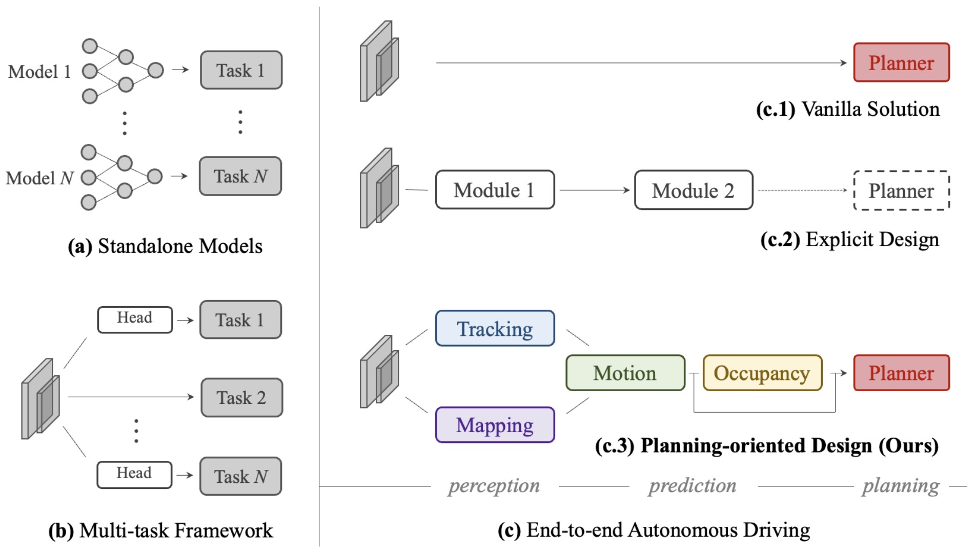
From Modular Pipelines to End-to-End Driving must be evaluated interactively because ego actions change the future traffic scene and can provoke different responses from other agents; fixed-log replay cannot capture those feedback effects.
At its core, end-to-end driving learns to map an observation history directly to a planned future trajectory:
\[I_{\leq t}\rightarrow\tau_{t:t+H}\]
Planning-oriented Autonomous Driving by Hu et al. (2022) introduced UniAD, integrating detection, tracking, mapping, motion forecasting, occupancy prediction, and planning into a unified network organized around planning.
A joint objective may be written as:
\[\mathcal{L}=\lambda_{\mathrm{det}}\mathcal{L}_{\mathrm{det}}+\lambda_{\mathrm{track}}\mathcal{L}_{\mathrm{track}}+\lambda_{\mathrm{map}}\mathcal{L}_{\mathrm{map}}+\lambda_{\mathrm{pred}}\mathcal{L}_{\mathrm{pred}}+\lambda_{\mathrm{plan}}\mathcal{L}_{\mathrm{plan}}\]

Scene Representations for Learned Driving

Scene Representations for Learned Driving must account for the fact that an autonomous vehicle changes the future scene through its own motion and through the reactions of other agents. Closed-loop evaluation is therefore essential for separating trajectories that look plausible in recorded logs from policies that remain safe and effective under interaction.
Scene Representations for Learned Driving must be evaluated interactively because ego actions change the future traffic scene and can provoke different responses from other agents; fixed-log replay cannot capture those feedback effects.
A dense representation might encode occupancy:
\[O(x,y,t)=P(\text{occupied}\mid x,y,t)\]
A vectorized representation instead represents individual scene elements:
\[S=\{V_1,\ldots,V_N,L_1,\ldots,L_M\}\]
VAD: Vectorized Scene Representation for Efficient Autonomous Driving by Jiang et al. (2023) represents agents and map elements as vectors and uses them as explicit planning constraints.

Driving as a Multimodal Prediction Problem

Driving as a Multimodal Prediction Problem must account for the fact that an autonomous vehicle changes the future scene through its own motion and through the reactions of other agents. Closed-loop evaluation is therefore essential for separating trajectories that look plausible in recorded logs from policies that remain safe and effective under interaction.
Driving as a Multimodal Prediction Problem should optimize for decision-relevant prediction: contact, geometry, timing, and task progress matter when they change which action is preferred, whereas visually conspicuous errors may be harmless if they do not affect control.
Driving behavior is inherently multimodal. A deterministic regression model minimizing:
\[\mathcal{L}=\|\tau-\hat\tau\|_2^2\]
- may average multiple valid modes.
  \[\boxed{\text{average of valid trajectories}\neq\text{valid trajectory}.}\]
A policy can instead represent:
\[p_\theta(\tau\mid o_{\leq t},n)\]

Prediction Is Interactive

In an interactive system, predictions alter the state from which the next observation is obtained, so errors compound through the policy-induced state distribution rather than remaining independent across timesteps.
Prediction Is Interactive should optimize for decision-relevant prediction: contact, geometry, timing, and task progress matter when they change which action is preferred, whereas visually conspicuous errors may be harmless if they do not affect control.
A conventional predictor estimates:
\[p(\tau_{\mathrm{others}}\mid o)\]
- while an interactive predictor considers:
  \[p(\tau_{\mathrm{others}}\mid o,\tau_{\mathrm{ego}})\]
Planning therefore becomes a coupled multi-agent problem:
\[\tau_{\mathrm{ego}}\leftrightarrow\tau_{\mathrm{others}}\]

Prediction and Closed-Loop Evaluation

This section connects open-loop versus closed-loop evaluation with vision-language models for driving. The discussion develops the relevant methods, implementation details, and practical tradeoffs.

Open-Loop Versus Closed-Loop Evaluation

Open-Loop Versus Closed-Loop Evaluation distinguishes replaying predictions against fixed recorded observations from executing actions that change subsequent observations; only the latter exposes policy-induced distribution shift and compounding errors.
Open-Loop Versus Closed-Loop Evaluation should separate prediction on fixed logs from interactive execution, since only the latter captures how the policy’s actions alter future observations and compound errors.
Open-loop evaluation compares a prediction with a recorded trajectory:
\[E_{\mathrm{open}}=d(\hat\tau,\tau^*)\]
Closed-loop evaluation instead executes the policy:
\[a_t\sim\pi_\theta(o_t),\qquad s_{t+1}\sim P(s_{t+1}\mid s_t,a_t)\]
Thus,
\[\boxed{\text{open loop evaluates predictions;}\qquad\text{closed loop evaluates behavior}.}\]

Why Long-Tail Scenarios Dominate Autonomous Driving

Why Long-Tail Scenarios Dominate Autonomous Driving must account for the fact that an autonomous vehicle changes the future scene through its own motion and through the reactions of other agents. Closed-loop evaluation is therefore essential for separating trajectories that look plausible in recorded logs from policies that remain safe and effective under interaction.
Why Long-Tail Scenarios Dominate Autonomous Driving must be evaluated interactively because ego actions change the future traffic scene and can provoke different responses from other agents; fixed-log replay cannot capture those feedback effects.
Routine driving is common while difficult edge cases are rare:
\[\mathcal{D}_{\mathrm{long-tail}}\ll\mathcal{D}_{\mathrm{routine}}\]
The challenge is therefore:
\[\boxed{\text{generalization under sparse supervision}}\]

Vision-Language Models for Driving

In autonomous driving, vision-language models contribute scene interpretation and causal reasoning, but useful deployment requires those representations to remain aligned with route context, ego state, dynamic actors, and the trajectory-generation interface.
Vision-Language Models for Driving should connect semantic intent to the current physical state and available actions, with execution feedback used to verify that the chosen interpretation actually produced the intended effect.
DriveVLM: The Convergence of Autonomous Driving and Large Vision-Language Models by Tian et al. (2024) introduced a VLM-based driving system organized around scene description, scene analysis, and hierarchical planning, together with DriveVLM-Dual.
A VLM may be effective at semantic reasoning but comparatively weak at precise spatial control, motivating hybrid architectures. In practice, the representation must preserve the task-relevant geometry, state, and uncertainty needed by downstream reasoning and control rather than only semantic appearance.

From Driving VLMs to Driving VLAs

A driving VLA closes the gap between scene understanding and vehicle control by predicting trajectories or control-relevant outputs from multimodal driving context, making closed-loop consequences part of the model’s effective objective.
From Driving VLMs to Driving VLAs should connect semantic intent to the current physical state and available actions, with execution feedback used to verify that the chosen interpretation actually produced the intended effect.
A driving VLA receives:
\[x_t=\{I_{\leq t}^{1:N},n_t,e_{\leq t}\}\]
- and can predict reasoning and action:
  \[\pi_\theta(r_t,\tau_t\mid x_t)\]
A Survey on Vision-Language-Action Models for Autonomous Driving by Jiang et al. (2025) characterizes this emerging class as integrating visual perception, language understanding, reasoning, and vehicle control.

NVIDIA Alpamayo

NVIDIA Alpamayo must account for the fact that an autonomous vehicle changes the future scene through its own motion and through the reactions of other agents. Closed-loop evaluation is therefore essential for separating trajectories that look plausible in recorded logs from policies that remain safe and effective under interaction.
NVIDIA Alpamayo must be evaluated interactively because ego actions change the future traffic scene and can provoke different responses from other agents; fixed-log replay cannot capture those feedback effects.
NVIDIA Alpamayo is a family of reasoning VLA models, simulation frameworks, and datasets for autonomous-driving development.
\[\boxed{\text{Alpamayo}+\text{AlpaSim}+\text{AlpaGym}}\]
The NVIDIA Alpamayo platform describes Alpamayo models as consuming multi-camera video, navigation inputs, and driving context and producing future trajectories and Chain-of-Causation reasoning traces. For embodied use, that semantic interpretation must remain tied to the current scene, the robot state, and the actions that are actually feasible for the embodiment.

Reasoning-Based Driving Models

This section connects Alpamayo 1 with why reasoning-action alignment matters. The discussion develops the relevant methods, implementation details, and practical tradeoffs.

Alpamayo 1

Alpamayo 1 must account for the fact that an autonomous vehicle changes the future scene through its own motion and through the reactions of other agents. Closed-loop evaluation is therefore essential for separating trajectories that look plausible in recorded logs from policies that remain safe and effective under interaction.
Alpamayo 1 must be evaluated interactively because ego actions change the future traffic scene and can provoke different responses from other agents; fixed-log replay cannot capture those feedback effects.
Alpamayo 1: Bridging Reasoning and Action Prediction for Generalizable Autonomous Driving in the Long Tail integrates explicit reasoning with trajectory prediction for difficult long-tail driving scenarios. For embodied use, that semantic interpretation must remain tied to the current scene, the robot state, and the actions that are actually feasible for the embodiment.
Conceptually,
\[h_t=f_{\mathrm{reason}}(I_{\leq t},n_t,e_{\leq t})\]
- followed by:
  \[\tau_t=f_{\mathrm{trajectory}}(h_t,\epsilon)\]

Chain of Causation Reasoning

Chain-of-Causation reasoning makes the factors behind a maneuver explicit, linking observed actors and constraints to a planned trajectory so driving decisions can be inspected alongside their physical outputs.
Chain of Causation Reasoning should connect semantic intent to the current physical state and available actions, with execution feedback used to verify that the chosen interpretation actually produced the intended effect.
Chain of Causation connects observations to causal factors that determine driving action:
\[\text{Observation}\rightarrow\text{Relevant Agent}\rightarrow\text{Predicted Interaction}\rightarrow\text{Driving Constraint}\rightarrow\text{Action}\]
Thus,
\[r_t\leftrightarrow\tau_t\]

Why Reasoning-Action Alignment Matters

Reasoning is useful only when it changes action selection in ways consistent with the current scene; a mismatch between the stated rationale and the executed trajectory can therefore expose a failure at the reasoning-control interface.
Why Reasoning-Action Alignment Matters should connect semantic intent to the current physical state and available actions, with execution feedback used to verify that the chosen interpretation actually produced the intended effect.
A model could produce plausible reasoning while independently producing an unrelated trajectory:
\[p(r,\tau\mid o)=p(r\mid o)p(\tau\mid o)\]
A reasoning VLA instead seeks strong consistency with a structure closer to:
\[o\rightarrow r\rightarrow\tau\]

Training Reasoning VLAs

Reasoning-oriented VLAs add supervision for intermediate causal or semantic structure alongside action targets, aiming to make trajectory generation depend on an explicit account of relevant agents, constraints, and intended maneuvers rather than visual pattern matching alone.
Training Reasoning VLAs should connect semantic intent to the current physical state and available actions, with execution feedback used to verify that the chosen interpretation actually produced the intended effect.
A simplified pipeline is:
\[\boxed{\text{Foundation Model}\rightarrow\text{Driving SFT}\rightarrow\text{Reasoning SFT}\rightarrow\text{RL}\rightarrow\text{Driving VLA}.}\]
A supervised objective can be represented as:
\[\mathcal{L}_{\mathrm{SFT}}=\lambda_r\mathcal{L}_{\mathrm{reason}}+\lambda_\tau\mathcal{L}_{\mathrm{trajectory}}\]
Reinforcement learning can optimize:
\[J(\pi)=\mathbb{E}_{\tau\sim\pi}[R(\tau,r)]\]

Trajectory Generation as an Action Expert

Trajectory Generation as an Action Expert must account for the fact that an autonomous vehicle changes the future scene through its own motion and through the reactions of other agents. Closed-loop evaluation is therefore essential for separating trajectories that look plausible in recorded logs from policies that remain safe and effective under interaction.
An action expert is useful when generated trajectories expand coverage of hard states while remaining consistent with the target robot’s dynamics and task constraints, not merely when they increase sample count.
A driving VLA often predicts a future trajectory:
\[\tau=[p_1,p_2,\ldots,p_H]\]
- where:
  \[p_k=(x_k,y_k,\theta_k)\]
A downstream controller computes:
\[u_t=f_{\mathrm{control}}(\tau,s_t)\]
Thus,
\[\boxed{\text{Reasoning}\rightarrow\text{Trajectory}\rightarrow\text{Control}\rightarrow\text{Actuation}.}\]

Training and Action Generation

This section connects diffusion-based trajectory prediction with foundation models as te. The discussion develops the relevant methods, implementation details, and practical tradeoffs.

Diffusion-Based Trajectory Prediction

Diffusion-Based Trajectory Prediction represents future motion as a distribution rather than a single deterministic path, which is useful when multiple maneuvers remain physically plausible from the same observation.
Diffusion-based trajectory models contribute data diversity by representing several plausible futures, but the training benefit depends on whether those samples preserve the geometry and dynamics that distinguish successful from unsafe motion.
Given noisy trajectory $\tau^k$, a diffusion decoder learns:
\[\epsilon_\theta(\tau^k,k,h)\]
A standard objective is:
\[\mathcal{L}_{\mathrm{diff}}=\mathbb{E}\left[\|\epsilon-\epsilon_\theta(\tau^k,k,h)\|_2^2\right]\]
At inference,
\[\tau^K\sim\mathcal{N}(0,I)\]
- is transformed into a physically plausible trajectory.

Alpamayo 1.5

Alpamayo 1.5 must account for the fact that an autonomous vehicle changes the future scene through its own motion and through the reactions of other agents. Closed-loop evaluation is therefore essential for separating trajectories that look plausible in recorded logs from policies that remain safe and effective under interaction.
Alpamayo 1.5 must be evaluated interactively because ego actions change the future traffic scene and can provoke different responses from other agents; fixed-log replay cannot capture those feedback effects.
The Alpamayo family subsequently expanded to Alpamayo 1.5, continuing the pattern:
\[\boxed{\text{Video + Navigation + Ego History}\rightarrow\text{Reasoning}\rightarrow\text{Trajectory}.}\]

Alpamayo 2 Super

Alpamayo 2 Super must account for the fact that an autonomous vehicle changes the future scene through its own motion and through the reactions of other agents. Closed-loop evaluation is therefore essential for separating trajectories that look plausible in recorded logs from policies that remain safe and effective under interaction.
Alpamayo 2 Super must be evaluated interactively because ego actions change the future traffic scene and can provoke different responses from other agents; fixed-log replay cannot capture those feedback effects.
NVIDIA announced Alpamayo 2 Super in May 2026 as part of the continuing Alpamayo family for autonomous-driving and robotaxi development. Closed-loop evaluation is especially important here because the planned trajectory changes the future traffic configuration that the policy will subsequently observe.
The broader scaling direction is:
\[\text{specialized planner}\rightarrow\text{driving foundation model}\]

Foundation Models as Teachers

Foundation Models as Teachers uses a larger model to supply semantic supervision, plans, labels, or trajectories that can train a smaller physical policy without requiring the teacher itself to meet deployment latency.
Foundation Models as Teachers should distinguish broadly reusable semantic and perceptual representations from robot-specific calibration in kinematics, dynamics, sensing, action ranges, and recovery behavior.
A large driving foundation model need not be the final deployed model. The design choice determines how much semantic knowledge can be shared across tasks while still preserving the precision and timing required by the robot-specific action interface.
For teacher $\pi_T$ and student $\pi_S$,
\[(r_T,\tau_T)\sim\pi_T(o)\]
- and the student can minimize:
  \[\mathcal{L}_{\mathrm{distill}}=\lambda_rD(r_S,r_T)+\lambda_\tau D(\tau_S,\tau_T)\]
Thus,
\[\boxed{\text{large foundation teacher}\rightarrow\text{distillation}\rightarrow\text{real-time driving policy}.}\]

AlpaSim

AlpaSim evaluates driving policies by applying their predicted actions inside an interactive simulator and rendering the resulting observations, exposing feedback effects that open-loop replay cannot capture.
AlpaSim should be evaluated through the behavior it produces after integration, because component-level metrics can miss timing, state-distribution, and control-interface failures that only appear in closed-loop execution.
AlpaSim is NVIDIA’s open-source closed-loop autonomous-driving simulation framework. Because each executed command changes the next input distribution, the relevant unit of evaluation is the resulting rollout rather than an isolated one-step prediction.
The simulator implements:
\[s_{t+1}=F_{\mathrm{sim}}(s_t,a_t)\]
- while the policy observes:
  \[o_t=O_{\mathrm{sim}}(s_t)\]
  - and produces:
    \[a_t=\pi_\theta(o_t)\]

Why Closed-Loop Simulation Changes the Optimization Problem

Why Closed-Loop Simulation Changes the Optimization Problem evaluates behavior through the feedback loop created when each action changes the next state and observation, exposing compounding errors that static prediction metrics can hide.
Why Closed-Loop Simulation Changes the Optimization Problem should vary or calibrate the physical and sensing factors that materially affect the deployed policy, with success measured by transfer to held-out real behavior rather than by simulator performance alone.
Trajectory similarity is not identical to driving quality:
\[\boxed{\text{trajectory similarity}\neq\text{driving quality}.}\]
A more appropriate objective is closer to:
\[R=R_{\mathrm{safety}}+R_{\mathrm{progress}}+R_{\mathrm{comfort}}+R_{\mathrm{rules}}+R_{\mathrm{interaction}}\]

Simulation and Reinforcement Learning

This section connects alpagym with counterfactual driving experience. The discussion develops the relevant methods, implementation details, and practical tradeoffs.

AlpaGym

AlpaGym turns closed-loop driving rollouts into reinforcement-learning experience, so the policy can be optimized on the consequences of its own steering and braking rather than only on logged expert trajectories.
AlpaGym should be evaluated through the behavior it produces after integration, because component-level metrics can miss timing, state-distribution, and control-interface failures that only appear in closed-loop execution.
AlpaGym connects model decisions with feedback from closed-loop simulation for reinforcement-learning post-training. Because each executed command changes the next input distribution, the relevant unit of evaluation is the resulting rollout rather than an isolated one-step prediction.
The learning loop is:
\[\pi_{\theta_k}\rightarrow\text{AlpaSim Rollout}\rightarrow R(\tau)\rightarrow\text{RL Update}\rightarrow\pi_{\theta_{k+1}}\]
Imitation learning seeks:
\[\pi_\theta\approx\pi_{\mathrm{human}}\]
- whereas reinforcement learning seeks:
  \[\pi_\theta=\arg\max_\pi\mathbb{E}[R(\tau)]\]

Closed-Loop RL for Driving

Closed-Loop RL for Driving trains on trajectories generated by the policy’s own steering and braking, allowing rewards to reflect downstream driving consequences that are absent from one-step imitation targets.
Closed-Loop RL for Driving must be evaluated interactively because ego actions change the future traffic scene and can provoke different responses from other agents; fixed-log replay cannot capture those feedback effects.
A reward can combine:
\[R(\tau)=w_sR_{\mathrm{safety}}+w_pR_{\mathrm{progress}}+w_cR_{\mathrm{comfort}}+w_rR_{\mathrm{rules}}\]
For example,
\[R_{\mathrm{safety}}=-\mathbb{1}[\text{collision}]\] \[R_{\mathrm{progress}}=d_{t-1}^{\mathrm{goal}}-d_t^{\mathrm{goal}}\]
- and:
  \[R_{\mathrm{comfort}}=-\sum_t\|j_t\|^2\]

Counterfactual Driving Experience

Counterfactual Driving Experience must account for the fact that an autonomous vehicle changes the future scene through its own motion and through the reactions of other agents. Closed-loop evaluation is therefore essential for separating trajectories that look plausible in recorded logs from policies that remain safe and effective under interaction.
Counterfactual Driving Experience should be judged by whether the model preserves the relative consequences of alternative actions, even if their rendered futures are not pixel-perfect.
Starting from state $s_t$, simulation can test candidate trajectories:
\[\tau^{(1)},\tau^{(2)},\ldots,\tau^{(K)}\]
Each produces a different future:
\[s_{t+H}^{(k)}=F(s_t,\tau^{(k)})\]
This transforms driving data from what happened into what could have happened. What matters is not only the number of examples but also their coverage of tasks, embodiments, recovery states, and observation-action alignments that the deployed policy will encounter.

World Models for Autonomous Driving

World Models for Autonomous Driving must predict interactive traffic futures conditioned on ego actions, because surrounding agents may react to the vehicle’s planned motion and invalidate open-loop forecasts.
World Models for Autonomous Driving should optimize for decision-relevant prediction: contact, geometry, timing, and task progress matter when they change which action is preferred, whereas visually conspicuous errors may be harmless if they do not affect control.
A driving world model estimates:
\[p_\phi(o_{t+1:t+H}\mid o_{\leq t},a_{t:t+H})\]
This creates the loop:
\[\boxed{\text{Driving Policy}\rightarrow\text{Candidate Action}\rightarrow\text{World Model}\rightarrow\text{Predicted Consequence}\rightarrow\text{Policy Improvement}.}\]

Neural Reconstruction and Digital Twins

Neural Reconstruction and Digital Twins turns recorded sensor data into an interactive scene representation, enabling repeatable viewpoint changes and policy tests while retaining much of the captured environment’s visual structure.
Neural Reconstruction and Digital Twins uses a scene-specific simulation surrogate to preserve geometry, sensing, and dynamics well enough to replay or perturb real failures for controlled regression testing.
Given fleet observations:
\[\{I_t,L_t,P_t\}_{t=1}^{T}\]
- a system can reconstruct a three-dimensional scene:
  \[\hat E=f_{\mathrm{reconstruct}}(I_{1:T},L_{1:T},P_{1:T})\]
The original scenario can then become a family of counterfactual scenarios:
\[E\rightarrow\{E_1,E_2,\ldots,E_N\}\]

Long-Tail Scenario Generation

Long-tail scenario generation is valuable when it deliberately increases coverage of rare interactions, boundary conditions, and safety-critical states rather than merely producing more nominal driving data.
Long-Tail Scenario Generation must be evaluated interactively because ego actions change the future traffic scene and can provoke different responses from other agents; fixed-log replay cannot capture those feedback effects.
A generative scenario engine can vary factors such as speed, visibility, pedestrian timing, road geometry, weather, and traffic density:
\[E_i=G(E_0,z_i)\]
The key objective is behaviorally meaningful scenario diversity. The training stage should therefore be interpreted by the capability it is intended to add: broad representations, embodiment grounding, task adaptation, or closed-loop behavioral improvement.

Data, Safety, and Deployment

This section connects the autonomous driving data engine with safety layers around learned policies. The discussion develops the relevant methods, implementation details, and practical tradeoffs.

The Autonomous Driving Data Engine

The Autonomous Driving Data Engine must account for the fact that an autonomous vehicle changes the future scene through its own motion and through the reactions of other agents. Closed-loop evaluation is therefore essential for separating trajectories that look plausible in recorded logs from policies that remain safe and effective under interaction.
The Autonomous Driving Data Engine should be assessed by the new behavioral coverage it contributes, especially rare states, recovery situations, and observation-action combinations that are missing from the current training distribution.
A modern Physical AI data engine can combine:
\[\mathcal{D}=\mathcal{D}_{\mathrm{fleet}}+\mathcal{D}_{\mathrm{human}}+\mathcal{D}_{\mathrm{sim}}+\mathcal{D}_{\mathrm{world-model}}+\mathcal{D}_{\mathrm{RL}}\]
The resulting loop is:
\[\boxed{\text{Deploy}\rightarrow\text{Mine Failures}\rightarrow\text{Reconstruct}\rightarrow\text{Generate Variants}\rightarrow\text{Simulate}\rightarrow\text{Post-Train}\rightarrow\text{Deploy}.}\]

Safety Is a Trajectory Property

Safety Is a Trajectory Property must account for the fact that an autonomous vehicle changes the future scene through its own motion and through the reactions of other agents. Closed-loop evaluation is therefore essential for separating trajectories that look plausible in recorded logs from policies that remain safe and effective under interaction.
Safety labels are most informative at the trajectory level because a locally acceptable action can create a later hazard through speed, contact, accumulated error, or an unrecoverable state transition.
A simple clearance constraint is:
\[d(\tau_{\mathrm{ego}}(t),\tau_i(t))>d_{\min}\]
Robust safety also involves uncertainty:
\[p(\tau_i\mid o_{\leq t})\]
A desired risk constraint is:
\[P(\text{collision}\mid\tau_{\mathrm{ego}})<\epsilon\]

Safety Layers Around Learned Policies

Safety Layers Around Learned Policies should be implemented as a system property rather than inferred from average policy success. Learned behavior, uncertainty estimates, runtime constraints, independent monitors, and fallback behavior provide complementary layers because they fail under different assumptions.
Safety Layers Around Learned Policies requires enforcement outside the learned policy for constraints that must hold even when the model is uncertain, out of distribution, or wrong.
A safety layer can transform nominal learned action:
\[a_t^{\mathrm{policy}}\]
- into:
  \[a_t^{\mathrm{safe}}=\mathcal{S}(a_t^{\mathrm{policy}},s_t)\]
This produces:
\[\boxed{\text{learned intelligence}+\text{independent safety envelope}.}\]

Reasoning Is Not a Safety Proof

Reasoning Is Not a Safety Proof should be implemented as a system property rather than inferred from average policy success. Learned behavior, uncertainty estimates, runtime constraints, independent monitors, and fallback behavior provide complementary layers because they fail under different assumptions.
Reasoning Is Not a Safety Proof requires enforcement outside the learned policy for constraints that must hold even when the model is uncertain, out of distribution, or wrong.
Natural-language reasoning can improve interpretability, training, and debugging, but:
\[\boxed{\text{explainability}\neq\text{verification}}\]
Reasoning traces should be evaluated for consistency with observed evidence and behavior, while trajectory safety should be evaluated independently. For embodied use, that semantic interpretation must remain tied to the current scene, the robot state, and the actions that are actually feasible for the embodiment.

The Driving Physical AI Stack

The Driving Physical AI Stack combines sensing, multimodal reasoning, action generation, simulation, and runtime safeguards into a single feedback system whose interfaces determine what information survives from perception to execution.
The Driving Physical AI Stack must be evaluated interactively because ego actions change the future traffic scene and can provoke different responses from other agents; fixed-log replay cannot capture those feedback effects.
The emerging architecture can be summarized as:
\[\boxed{ \begin{array}{c} \text{Fleet + Synthetic + Simulation Data}\\ \downarrow\\ \text{Multimodal Foundation Model}\\ \downarrow\\ \text{Scene Reasoning}\\ \downarrow\\ \text{Trajectory Action Expert}\\ \downarrow\\ \text{Safety / Control Layer}\\ \downarrow\\ \text{Vehicle}\\ \downarrow\\ \text{Closed-Loop Environment}\\ \downarrow\\ \text{New Experience}\\ \circlearrowleft \end{array} }\]
The transition from classical autonomous driving to Physical AI includes shifts from hand-designed to learned representations, separate modules to jointly optimized systems, trajectory imitation to reasoning plus generative planning, open-loop evaluation to closed-loop simulation, and offline supervised learning to closed-loop post-training.
The result is an increasingly general development pattern:
\[\boxed{\text{Reason}\rightarrow\text{Act}\rightarrow\text{Simulate Consequences}\rightarrow\text{Learn}}\]
The next section will examine World Models for Physical AI in detail, including predictive dynamics, latent world models, model-based reinforcement learning, Dreamer, Cosmos, video world models, neural reconstruction, digital twins, counterfactual simulation, and how world models can become learned environments for training physical agents.
It will also include the requested reference to our World Models primer for a more detailed treatment of VLAs and World Models. Its usefulness therefore depends less on visual plausibility alone than on whether predicted state changes preserve the consequences that would alter a downstream decision.

World Models for Physical AI

World models predict the consequences of actions and support planning, training, and evaluation. This chapter moves from latent dynamics to generative simulation and integration with robot policies.
A detailed discourse on World Modeling is available in our World Modeling primer.

World-Model Foundations

This section develops why physical agents need world models in the context of the broader Physical AI system. It connects the underlying concepts to the implementation details discussed below.

Why Physical Agents Need World Models

Why Physical Agents Need World Models models how physical state evolves under actions, enabling counterfactual prediction, planning, synthetic experience, and closed-loop evaluation before every decision is attempted in the real world.
Why Physical Agents Need World Models should optimize for decision-relevant prediction: contact, geometry, timing, and task progress matter when they change which action is preferred, whereas visually conspicuous errors may be harmless if they do not affect control.
A policy answers:
\[\text{What should I do?}\]
A world model answers a different question:
\[\text{What is likely to happen if I do it?}\]
For an agent interacting with a physical environment, this distinction is fundamental. A policy maps observations and goals to actions,
\[a_t \sim \pi_\theta(a_t\mid o_{\leq t},g)\]
- while a world model approximates the environment’s dynamics,
  \[p_\phi(s_{t+1}\mid s_t,a_t)\]
  - or, over a longer horizon,
    \[p_\phi(s_{t+1:t+H}\mid s_t,a_{t:t+H-1})\]
The model can therefore simulate possible consequences before the agent commits to them in the physical world. World Models by Ha and Schmidhuber (2018) demonstrated the core idea using learned compressed spatial and temporal representations, including training a controller inside trajectories generated by the learned environment model.
A substantially more detailed treatment of world models, JEPA-style predictive learning, and their relationship to Vision-Language-Action models is available in our World Models primer. In practice, the representation must preserve the task-relevant geometry, state, and uncertainty needed by downstream reasoning and control rather than only semantic appearance.

World Models as Learned Dynamics

World Models as Learned Dynamics models how physical state evolves under actions, enabling counterfactual prediction, planning, synthetic experience, and closed-loop evaluation before every decision is attempted in the real world.
World Models as Learned Dynamics should optimize for decision-relevant prediction: contact, geometry, timing, and task progress matter when they change which action is preferred, whereas visually conspicuous errors may be harmless if they do not affect control.
Consider an environment with latent state $s_t$ action $a_t$ and observation $o_t$. The physical environment evolves according to an unknown transition function:
\[s_{t+1} \sim P( s_{t+1}\mid s_t,a_t )\]
A learned world model approximates this distribution:
\[\hat P_\phi( s_{t+1}\mid s_t,a_t ) \approx P( s_{t+1}\mid s_t,a_t )\]
In partially observed environments, the agent does not have direct access to $s_t$. Instead, an encoder constructs a latent representation:
\[z_t = f_\phi( o_{\leq t} )\]
The dynamics model then predicts:
\[\hat z_{t+1} = g_\phi( z_t,a_t )\]
A decoder may optionally reconstruct observations:
\[\hat o_{t+1} = d_\phi( \hat z_{t+1} )\]
This gives the canonical learned dynamics pipeline:
\[\boxed{ o_t \rightarrow z_t \xrightarrow{a_t} z_{t+1} \rightarrow o_{t+1}. }\]

Why Predict in Latent Space?

Latent dynamics models compress observations before predicting future state, reducing rollout cost and allowing planning to focus on task-relevant structure instead of reconstructing every pixel at every step.
Why Predict in Latent Space? is useful only if compression preserves the variables that change rewards and action rankings; high reconstruction quality is neither necessary nor sufficient for that decision-level requirement.
Predicting every pixel of the future can force a model to allocate capacity to details irrelevant to action. Suppose a robot moves toward a cup. The future image may depend on shadows, reflections, textures, background motion, sensor noise, and lighting.
Yet the controller may primarily need to know:
\[\text{cup pose}, \quad \text{gripper pose}, \quad \text{contact state}, \quad \text{collision geometry}\]
A latent world model instead learns:
\[z_t=f(o_t)\]
- and predicts:
  \[z_{t+1}=g(z_t,a_t)\]
The objective can be:
\[\mathcal{L}_{\mathrm{pred}} = \| g_\phi(z_t,a_t) - \operatorname{sg}(z_{t+1}) \|_2^2\]
- where $\operatorname{sg}$ denotes stop-gradient.
The desired latent space preserves information useful for future prediction and control while discarding irrelevant visual variability. In practice, the representation must preserve the task-relevant geometry, state, and uncertainty needed by downstream reasoning and control rather than only semantic appearance.

Observation Models Versus State Models

Observation Models Versus State Models prevents representational mismatches from being mistaken for learning problems. Units, coordinate frames, action conventions, timing, padding, and embodiment metadata must remain explicit so heterogeneous examples describe comparable physical quantities.
Observation Models Versus State Models should be evaluated through the behavior it produces after integration, because component-level metrics can miss timing, state-distribution, and control-interface failures that only appear in closed-loop execution.
World models can operate at several levels.
A pixel-space model predicts:
\[p( o_{t+1} \mid o_{\leq t},a_t )\]
A latent model predicts:
\[p( z_{t+1} \mid z_t,a_t )\]
A structured state model may instead predict explicit quantities such as:
\[s_t = [ p_{\mathrm{objects}}, v_{\mathrm{objects}}, q_{\mathrm{robot}}, \dot q_{\mathrm{robot}}, c_{\mathrm{contacts}} ]\]
Each representation has different advantages. Pixel models can preserve rich visual information. Structured models provide interpretable physical state. Latent models can learn compact representations without requiring manually defined state variables.
Modern foundation world models increasingly combine these ideas by learning rich latent dynamics while retaining the ability to decode photorealistic observations. In practice, the representation must preserve the task-relevant geometry, state, and uncertainty needed by downstream reasoning and control rather than only semantic appearance.

Deterministic Versus Stochastic Dynamics

Stochastic dynamics are necessary when the same observed state can lead to several plausible futures, whereas deterministic predictors risk collapsing uncertainty into a single trajectory that may be overconfident.
Deterministic Versus Stochastic Dynamics should preserve multiple plausible futures when the environment is uncertain, because a single averaged prediction can conceal low-probability outcomes that dominate risk-sensitive decisions.
A deterministic model assumes:
\[z_{t+1} = f_\phi(z_t,a_t)\]
But physical environments often contain uncertainty. A pedestrian may turn left or right. An object may slip or remain stable. Another robot may respond in several plausible ways.
A stochastic world model instead learns:
\[p_\phi( z_{t+1} \mid z_t,a_t )\]
Over multiple timesteps,
\[p_\phi( z_{t+1:t+H} \mid z_t,a_{t:t+H-1} )\]
- represents a distribution over possible futures.
This distinction matters because
\[\boxed{ \text{one predicted future} \neq \text{the distribution of plausible futures}. }\]
Physical planning should often reason over the latter. For embodied use, that semantic interpretation must remain tied to the current scene, the robot state, and the actions that are actually feasible for the embodiment.

Multi-Step Prediction

Multi-step rollout quality matters because small one-step errors can accumulate into physically inconsistent futures, so useful world models must preserve decision-relevant structure across the horizon on which actions are compared.
Multi-Step Prediction exposes compounding model error over the same horizon used for planning, which is more relevant to control than isolated one-step prediction accuracy.
One-step accuracy is not sufficient for planning. A useful plan therefore has to connect high-level intent to reachable intermediate states and leave room to replan when execution produces an unexpected observation.
A world model used for decision making must recursively predict:
\[\hat z_{t+1} = f_\phi(z_t,a_t)\] \[\hat z_{t+2} = f_\phi(\hat z_{t+1},a_{t+1})\]
- and eventually:
  \[\hat z_{t+H}\]
Small errors can compound:
\[\epsilon_{t+H} \approx \sum_{k=1}^{H} J_k\epsilon_{t+k}\]
- where $J_k$ represents how prediction errors propagate through the learned dynamics.
Long-horizon consistency is therefore one of the central challenges in world-model research. Maintaining this context is important because delayed effects, partial observability, and earlier execution errors can all change which action is appropriate at the current step.

Model-Based Reinforcement Learning

Model-Based Reinforcement Learning supports reinforcement learning by producing imagined or simulated experience in which policies can explore consequences more cheaply than on hardware, subject to the risk of exploiting model errors.
Model-Based Reinforcement Learning depends on the feedback channel available during adaptation: offline supervision favors conservative updates within known data, whereas interactive feedback can correct new failure states at the cost of additional exploration and safety management.
Once an agent possesses a learned dynamics model, it can use that model to improve its policy. This is the central idea of model-based reinforcement learning.
Instead of obtaining every trajectory from the real environment,
\[\tau \sim P_{\mathrm{real}}\]
- the agent can generate imagined trajectories:
  \[\hat\tau \sim P_\phi\]
A candidate action sequence:
\[A = [ a_t,\ldots,a_{t+H-1} ]\]
- can be evaluated by rolling it through the model:
  \[\hat s_{t+k+1} \sim P_\phi( \hat s_{t+k+1} \mid \hat s_{t+k}, a_{t+k} )\]
The planner then estimates:
\[J(A) = \sum_{k=0}^{H-1} \gamma^k r( \hat s_{t+k}, a_{t+k} )\]
Planning selects:
\[A^* = \arg\max_A J(A)\]
Only the first action may be executed:
\[a_t=A_0^*\]
The agent then observes the real environment and replans. A useful plan therefore has to connect high-level intent to reachable intermediate states and leave room to replan when execution produces an unexpected observation.
This is learned model-predictive control.

Learning and Planning with Latent Dynamics

This section connects planning by imagination with dreamer. The discussion develops the relevant methods, implementation details, and practical tradeoffs.

Planning by Imagination

Planning by Imagination must account for the fact that an autonomous vehicle changes the future scene through its own motion and through the reactions of other agents. Closed-loop evaluation is therefore essential for separating trajectories that look plausible in recorded logs from policies that remain safe and effective under interaction.
Planning by Imagination should optimize for decision-relevant prediction: contact, geometry, timing, and task progress matter when they change which action is preferred, whereas visually conspicuous errors may be harmless if they do not affect control.
A world model transforms planning into counterfactual search. A useful plan therefore has to connect high-level intent to reachable intermediate states and leave room to replan when execution produces an unexpected observation.
Given current state $s_t$, consider candidate futures
\[A^{(1)},A^{(2)},\ldots,A^{(K)}\]
The world model generates:
\[\hat\tau^{(k)} = M_\phi( s_t,A^{(k)} )\]
A reward or value model evaluates each rollout:
\[V_k = R( \hat\tau^{(k)} )\]
The agent selects:
\[k^* = \arg\max_k V_k\]
Conceptually,
\[\boxed{ \text{Imagine} \rightarrow \text{Evaluate} \rightarrow \text{Act} }\]
This resembles human mental simulation: considering possible consequences before acting. A useful plan therefore has to connect high-level intent to reachable intermediate states and leave room to replan when execution produces an unexpected observation.

Dreamer

Dreamer learns a compact dynamics model and improves the policy through imagined latent trajectories, making model-generated experience part of the reinforcement-learning loop rather than only an auxiliary prediction task.
Dreamer should optimize for decision-relevant prediction: contact, geometry, timing, and task progress matter when they change which action is preferred, whereas visually conspicuous errors may be harmless if they do not affect control.
Mastering Diverse Domains through World Models by Hafner et al. (2023) introduced DreamerV3, which learns a world model and trains behavior using imagined trajectories generated within its learned latent dynamics; the same configuration was demonstrated across more than 150 tasks.
The following figure (source) shows DreamerV3 training: sensory inputs are encoded into latent dynamics, while actor and critic learn from imagined trajectories. Specifically, the world model encodes sensory inputs into discrete representations $z_t$ that are predicted by a sequence model with recurrent state $h_t$ given actions $a_t$. The inputs are reconstructed to shape the representations. The actor and critic predict actions $a_t$ and values $v_t$ and learn from trajectories of abstract representations predicted by the world model.

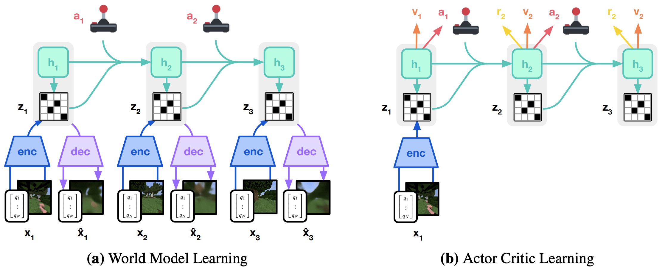
Dreamer’s architecture can be summarized as:
\[o_t \rightarrow z_t \rightarrow \text{latent dynamics} \rightarrow \hat z_{t+1:t+H}\]
An actor $\pi_\theta(a_t\mid z_t)$ and critic $V_\psi(z_t)$ are trained using imagined trajectories. The training stage should therefore be interpreted by the capability it is intended to add: broad representations, embodiment grounding, task adaptation, or closed-loop behavioral improvement.
Rather than repeatedly querying the physical environment, policy optimization occurs largely inside
\[\boxed{ \text{learned latent imagination} }\]
This substantially increases data efficiency when real interaction is expensive. This is the point where learned predictions meet coordinate frames, control rates, actuator limits, and the closed-loop dynamics of the physical system.

Representation, Dynamics, Reward, and Continuation Models

Separating representation, transition, reward, and continuation predictions lets a latent world model learn the quantities needed for imagined control without requiring every internal state to reconstruct the observation exactly.
Representation, Dynamics, Reward, and Continuation Models should optimize for decision-relevant prediction: contact, geometry, timing, and task progress matter when they change which action is preferred, whereas visually conspicuous errors may be harmless if they do not affect control.
A practical latent world model often contains several components. Its usefulness therefore depends less on visual plausibility alone than on whether predicted state changes preserve the consequences that would alter a downstream decision.
The encoder maps observations to representations:
\[z_t=f_{\mathrm{enc}}(o_t)\]
The dynamics model predicts future latent states:
\[z_{t+1} \sim p_\phi( z_{t+1}\mid z_t,a_t )\]
A reward model predicts:
\[\hat r_t = f_r(z_t,a_t)\]
A continuation model may predict whether the episode continues:
\[\hat c_t = P( \text{continue}\mid z_t )\]
The learned simulator can therefore provide most of the information required for reinforcement learning:
\[\boxed{ \text{state} + \text{transition} + \text{reward} + \text{termination} }\]

World Models as Data Generators

World Models as Data Generators turns learned dynamics into a source of additional experience, allowing targeted counterfactual trajectories to supplement expensive real interaction when their fidelity is sufficient for the downstream policy.
World Models as Data Generators should be assessed by the new behavioral coverage it contributes, especially rare states, recovery situations, and observation-action combinations that are missing from the current training distribution.
World models can also generate training data rather than directly controlling a policy. This is the point where learned predictions meet coordinate frames, control rates, actuator limits, and the closed-loop dynamics of the physical system.
Suppose a robot dataset contains:
\[\mathcal{D}_{\mathrm{real}} = \{ \tau_1,\ldots,\tau_N \}\]
A generative world model can produce additional trajectories:
\[\mathcal{D}_{\mathrm{synthetic}} = \{ \hat\tau_1,\ldots,\hat\tau_M \}\]
Training then uses:
\[\mathcal{D} = \mathcal{D}_{\mathrm{real}} \cup \mathcal{D}_{\mathrm{synthetic}}\]
This creates a different use of a world model:
\[\boxed{ \text{World Model} \rightarrow \text{Synthetic Experience} \rightarrow \text{Policy Training} }\]
The GR00T-Dreams and DreamGen workflows discussed earlier are examples of this broader pattern. Its usefulness therefore depends less on visual plausibility alone than on whether predicted state changes preserve the consequences that would alter a downstream decision.

Video Generation Becomes World Modeling

Video Generation Becomes World Modeling reframes video generation as action-conditioned prediction: the model is valuable when generated futures respond coherently to interventions rather than merely looking plausible.
Video Generation Becomes World Modeling should optimize for decision-relevant prediction: contact, geometry, timing, and task progress matter when they change which action is preferred, whereas visually conspicuous errors may be harmless if they do not affect control.
A conventional video generator models:
\[p( I_{t+1:T} \mid I_{\leq t},c )\]
- where $c$ might be text.
A world model becomes substantially more useful for Physical AI when generation is conditioned on actions:
\[p( I_{t+1:T} \mid I_{\leq t},a_{t:T},c )\]
The distinction is crucial:
- A video model asks:
  \[\text{What might happen next?}\]
- An action-conditioned world model asks:
  \[\text{What might happen if the agent does this?}\]
Thus,
\[\boxed{ \text{video prediction} + \text{action conditioning} \rightarrow \text{interactive world modeling} }\]

Foundation World Models

Foundation World Models seeks reusable predictive structure across many scenes and tasks, so a broadly pretrained dynamics model can be adapted into specialized simulators or policy components rather than learned from scratch for each domain.
Foundation World Models should optimize for decision-relevant prediction: contact, geometry, timing, and task progress matter when they change which action is preferred, whereas visually conspicuous errors may be harmless if they do not affect control.
Traditional world models are often trained for one environment. A foundation world model instead seeks a broad prior over physical environments:
\[p_\phi( \text{future} \mid \text{history}, \text{actions}, \text{context} )\]
The model can then be adapted to a specific downstream environment:
\[M_{\mathrm{foundation}} \xrightarrow{\mathrm{post\text{-}training}} M_{\mathrm{domain}}\]
This mirrors the transition from task-specific language models to LLMs and from task-specific robot policies to VLAs. For embodied use, that semantic interpretation must remain tied to the current scene, the robot state, and the actions that are actually feasible for the embodiment.
The desired progression is:
\[\boxed{ \text{task-specific simulator} \rightarrow \text{world foundation model} \rightarrow \text{specialized physical simulator} }\]

NVIDIA Cosmos

Cosmos treats world modeling as reusable infrastructure for Physical AI, supporting controllable future generation, synthetic-data creation, and post-training for robotics and autonomous-system applications.
NVIDIA Cosmos should optimize for decision-relevant prediction: contact, geometry, timing, and task progress matter when they change which action is preferred, whereas visually conspicuous errors may be harmless if they do not affect control.
Cosmos World Foundation Model Platform for Physical AI by NVIDIA et al. (2025) introduced an open platform for building customized world models for Physical AI, including pretrained world foundation models, video tokenizers, data-curation infrastructure, and post-training workflows.
Cosmos explicitly frames Physical AI as requiring two complementary learned systems:
\[\boxed{ \text{policy model} + \text{world model} }\]
The policy approximates:
\[\pi_\theta( a_t \mid o_{\leq t},g )\]
- while the world model approximates
  \[p_\phi( o_{t+1:t+H} \mid o_{\leq t}, a_{t:t+H-1} )\]
Together, they form an agent-environment pair that can increasingly be trained and evaluated digitally before deployment into the physical world. The training stage should therefore be interpreted by the capability it is intended to add: broad representations, embodiment grounding, task adaptation, or closed-loop behavioral improvement.

Generative and Foundation World Models

This section connects the cosmos data pipeline with video tokenization. The discussion develops the relevant methods, implementation details, and practical tradeoffs.

The Cosmos Data Pipeline

A world-model data pipeline must curate temporally coherent, physically meaningful video at scale because model quality depends as much on the distribution and cleanliness of trajectories as on the generative architecture.
The Cosmos Data Pipeline should be assessed by the new behavioral coverage it contributes, especially rare states, recovery situations, and observation-action combinations that are missing from the current training distribution.
World foundation models require enormous quantities of video. However,
\[\text{raw video} \neq \text{high-quality physical training data}\]
A scalable pipeline must perform operations such as:
\[\text{ingestion} \rightarrow \text{filtering} \rightarrow \text{deduplication} \rightarrow \text{captioning} \rightarrow \text{quality scoring} \rightarrow \text{sharding}\]
Cosmos therefore treats data curation as part of the world-model platform rather than as a preprocessing detail. What matters is not only the number of examples but also their coverage of tasks, embodiments, recovery states, and observation-action alignments that the deployed policy will encounter.
This mirrors the broader Physical AI pattern:
\[\boxed{ \text{model capability} \approx f( \text{architecture}, \text{data engine}, \text{post-training} ). }\]

Video Tokenization

Video tokenization determines the spatial and temporal information retained before world-model training, creating a tradeoff between compression efficiency and preservation of motion, geometry, and interaction details.
Video Tokenization changes how the policy represents and executes motion, so the chosen temporal horizon and action parameterization must remain compatible with controller rate, embodiment limits, and opportunities for feedback correction.
High-resolution video is computationally expensive. What matters is not only the number of examples but also their coverage of tasks, embodiments, recovery states, and observation-action alignments that the deployed policy will encounter.
Suppose a video tensor has shape:
\[T\times H\times W\times C\]
A tokenizer compresses it into latent tokens:
\[V \xrightarrow{\mathrm{encoder}} Z\]
If the compression ratio is $r$,
\[|Z| \ll |V|\]
The generative model operates in this compressed space:
\[p_\theta( Z_{t+1:T} \mid Z_{\leq t},c )\]
A decoder reconstructs video:
\[\hat V = D(Z)\]
Efficient tokenization is therefore a foundational systems problem for large-scale world modeling. Its usefulness therefore depends less on visual plausibility alone than on whether predicted state changes preserve the consequences that would alter a downstream decision.

Diffusion World Models

Diffusion World Models applies generative denoising to future-state prediction, allowing the model to represent several plausible physical evolutions instead of collapsing uncertainty into one forecast.
Diffusion World Models should optimize for decision-relevant prediction: contact, geometry, timing, and task progress matter when they change which action is preferred, whereas visually conspicuous errors may be harmless if they do not affect control.
Many modern visual world models use diffusion-style generation. In practice, the representation must preserve the task-relevant geometry, state, and uncertainty needed by downstream reasoning and control rather than only semantic appearance.
Starting with clean latent future $z_0$,
\[z_k = \sqrt{\bar\alpha_k}z_0 + \sqrt{1-\bar\alpha_k}\epsilon\]
The model learns:
\[\epsilon_\theta( z_k,k,c )\]
- under:
  \[\mathcal{L}_{\mathrm{diff}} = \mathbb{E} \left[ \| \epsilon-\epsilon_\theta(z_k,k,c) \|_2^2 \right]\]
For an action-conditioned model $c = \{o_{\leq t},a_{t:t+H},l\}$, the resulting generated future depends explicitly on the behavior being simulated. This is the point where learned predictions meet coordinate frames, control rates, actuator limits, and the closed-loop dynamics of the physical system.

Google DeepMind Genie

Genie-style world models learn action-controllable environments from visual experience, reframing generative video as a substrate for interactive agent training rather than only passive media synthesis.
Google DeepMind Genie should optimize for decision-relevant prediction: contact, geometry, timing, and task progress matter when they change which action is preferred, whereas visually conspicuous errors may be harmless if they do not affect control.
Genie: Generative Interactive Environments by Bruce et al. (2024) introduced an 11B-parameter generative interactive environment trained from unlabeled internet video, combining a spatiotemporal video tokenizer, autoregressive dynamics model, and latent action model. A particularly important idea is latent action discovery.
Given observations $o_t,o_{t+1}$ the model can infer latent action:
\[\hat a_t = f_{\mathrm{latent}} ( o_t,o_{t+1} )\]
This provides a mechanism for learning controllable dynamics even when internet video does not contain explicit action labels. This is the point where learned predictions meet coordinate frames, control rates, actuator limits, and the closed-loop dynamics of the physical system.
The conceptual transformation is:
\[\boxed{ \text{unlabeled video} \rightarrow \text{latent actions} \rightarrow \text{interactive environment} }\]

Genie 2

Genie 2 explores generative interactive environments in which actions condition future observations, providing a mechanism for producing diverse worlds that can be used for agent experience and evaluation.
Genie 2 should optimize for decision-relevant prediction: contact, geometry, timing, and task progress matter when they change which action is preferred, whereas visually conspicuous errors may be harmless if they do not affect control.
Genie 2: A large-scale foundation world model extended this direction to action-controllable 3D environments that can be generated from an initial image and interacted with by humans or agents. In practice, the representation must preserve the task-relevant geometry, state, and uncertainty needed by downstream reasoning and control rather than only semantic appearance.
Its inference loop can be represented as:
\[z_{t+1} \sim p_\phi( z_{t+1} \mid z_{\leq t},a_t )\]
After decoding,
\[I_{t+1} = D(z_{t+1})\]
The agent then chooses another action:
\[a_{t+1} = \pi( I_{\leq t+1} )\]
Thus the generated environment becomes interactive rather than a predetermined video. What matters is not only the number of examples but also their coverage of tasks, embodiments, recovery states, and observation-action alignments that the deployed policy will encounter.

Genie 3 and Real-Time Interactive Worlds

Interactive world models such as Genie 3 move from offline video generation toward environments that react continuously to actions, making temporal consistency and controllability central evaluation criteria.
Genie 3 and Real-Time Interactive Worlds should optimize for decision-relevant prediction: contact, geometry, timing, and task progress matter when they change which action is preferred, whereas visually conspicuous errors may be harmless if they do not affect control.
Genie 3: A new frontier for world models extends foundation world modeling toward longer-lived, real-time interactive environments generated from text prompts. For embodied use, that semantic interpretation must remain tied to the current scene, the robot state, and the actions that are actually feasible for the embodiment.
The trajectory is significant:
\[\text{video generation} \rightarrow \text{interactive video} \rightarrow \text{persistent generated environment}\]
A sufficiently capable interactive world model begins to function as a learned simulator. Its usefulness therefore depends less on visual plausibility alone than on whether predicted state changes preserve the consequences that would alter a downstream decision.
Instead of constructing every training environment manually,
\[E_i = \text{human-designed simulator}\]
- one can imagine generating environments from descriptions:
  \[E_i \sim p_\phi( E\mid\text{prompt} )\]
This could make environment generation itself scalable.

World Models as Infinite Curricula

World Models as Infinite Curricula models how physical state evolves under actions, enabling counterfactual prediction, planning, synthetic experience, and closed-loop evaluation before every decision is attempted in the real world.
World Models as Infinite Curricula should optimize for decision-relevant prediction: contact, geometry, timing, and task progress matter when they change which action is preferred, whereas visually conspicuous errors may be harmless if they do not affect control.
Suppose an agent struggles with a particular capability:
\[c = \text{opening unfamiliar doors}\]
A generative world model could construct environments $E_1,E_2,\ldots,E_N$ containing variations of that challenge. Its usefulness therefore depends less on visual plausibility alone than on whether predicted state changes preserve the consequences that would alter a downstream decision.
The agent trains:
\[\pi_k \xrightarrow{E_{1:N}} \pi_{k+1}\]
Failures are identified:
\[F_{k+1} = \operatorname{Failures}( \pi_{k+1} )\]
The world model then generates new environments concentrated around those failures:
\[E_{N+1:N+M} \sim p_\phi( E\mid F_{k+1} )\]
The resulting loop is:
\[\boxed{ \text{Agent} \rightarrow \text{Failures} \rightarrow \text{World Generation} \rightarrow \text{Training} \rightarrow \text{Agent} }\]
This turns environment generation into part of the learning algorithm. Its usefulness therefore depends less on visual plausibility alone than on whether predicted state changes preserve the consequences that would alter a downstream decision.

Interactive Simulation and Evaluation

This section connects counterfactual simulation with world models for policy evaluation. The discussion develops the relevant methods, implementation details, and practical tradeoffs.

Counterfactual Simulation

Counterfactual Simulation evaluates alternative actions from the same starting state, giving the agent information that logged experience cannot provide because only one action was actually taken in the recorded trajectory.
Counterfactual Simulation should vary or calibrate the physical and sensing factors that materially affect the deployed policy, with success measured by transfer to held-out real behavior rather than by simulator performance alone.
One of the most important capabilities of a world model is generating alternative futures from the same state. Its usefulness therefore depends less on visual plausibility alone than on whether predicted state changes preserve the consequences that would alter a downstream decision.
Given $s_t$, consider actions:
\[a_t^{(1)}, a_t^{(2)},\ldots,a_t^{(K)}\]
The model generates:
\[\hat s_{t+1:t+H}^{(k)} \sim p_\phi( s_{t+1:t+H} \mid s_t,a_t^{(k)} )\]
The agent can evaluate each outcome. This is especially valuable when real-world exploration is expensive or unsafe. A robot need not physically attempt every grasp. An autonomous vehicle need not physically execute every evasive maneuver.

The world model allows the system to ask $\boxed{\text{What if?}}$ before acting.

World Models for Policy Evaluation

World Models for Policy Evaluation should be judged by whether predicted futures rank or reject candidate actions correctly, not only by pixel similarity, because small visual errors may be harmless while small contact errors can reverse a control decision.
World Models for Policy Evaluation should optimize for decision-relevant prediction: contact, geometry, timing, and task progress matter when they change which action is preferred, whereas visually conspicuous errors may be harmless if they do not affect control.
Suppose two candidate policies are $\pi_A$ and $\pi_B$.
Instead of immediately deploying both physically, a world model can generate $\tau_A \sim M_\phi(\pi_A)$ and $\tau_B \sim M_\phi(\pi_B)$. This is the point where learned predictions meet coordinate frames, control rates, actuator limits, and the closed-loop dynamics of the physical system.
An evaluator computes:
\[R_A = R(\tau_A)\] \[R_B = R(\tau_B)\]
This enables rapid iteration. However, this procedure is trustworthy only when the world model is accurate in the regions visited by the evaluated policies.

Model Exploitation

A policy trained against a learned world model can exploit inaccuracies in that model, so high predicted reward is not sufficient unless the corresponding behavior remains valid under a more faithful simulator or real environment.
Model exploitation occurs when the policy discovers unrealistic behaviors that look successful only under world-model errors, so imagined gains must be checked in a stronger simulator or the real environment.
A central failure mode of model-based RL occurs when the policy discovers inaccuracies in the learned model. This is the point where learned predictions meet coordinate frames, control rates, actuator limits, and the closed-loop dynamics of the physical system.
Suppose:
\[\hat R(s,a) > R_{\mathrm{real}}(s,a)\]
Optimization may deliberately seek such regions:
\[\pi^* = \arg\max_\pi \mathbb{E}_{M_\phi}[R]\]
The policy then succeeds inside the learned simulator while failing in reality. This is model exploitation. The problem becomes more severe as optimization pressure increases:
\[\boxed{ \text{stronger optimizer} + \text{imperfect model} \rightarrow \text{greater exploitation risk}. }\]
World-model-based policy improvement therefore requires uncertainty estimation, real-world validation, and mechanisms for keeping imagined trajectories near regions where the model is reliable. This is the point where learned predictions meet coordinate frames, control rates, actuator limits, and the closed-loop dynamics of the physical system.

Uncertainty-Aware World Models

Uncertainty-Aware World Models should represent uncertainty over plausible futures so planning can distinguish robust actions from choices whose predicted success depends on one fragile forecast.
Uncertainty-Aware World Models should optimize for decision-relevant prediction: contact, geometry, timing, and task progress matter when they change which action is preferred, whereas visually conspicuous errors may be harmless if they do not affect control.
A useful world model should represent not only predictions but confidence. Its usefulness therefore depends less on visual plausibility alone than on whether predicted state changes preserve the consequences that would alter a downstream decision.
One approach uses an ensemble:
\[\{ M_{\phi_1},\ldots,M_{\phi_K} \}\]
For candidate transition $x$, disagreement:
\[U(x) = \operatorname{Var}_k [ M_{\phi_k}(x) ]\]
- can approximate epistemic uncertainty.
Planning can penalize uncertain trajectories:
\[J(\tau) = R(\tau) - \lambda U(\tau)\]
The agent therefore prefers high-reward futures that the world model also understands. Its usefulness therefore depends less on visual plausibility alone than on whether predicted state changes preserve the consequences that would alter a downstream decision.

The Reality Gap

The reality gap arises when simulation omits visual, dynamical, or interaction details that a deployed policy relies on; effective transfer therefore depends on matching or randomizing the factors that materially affect behavior.
The Reality Gap should be evaluated through the behavior it produces after integration, because component-level metrics can miss timing, state-distribution, and control-interface failures that only appear in closed-loop execution.
World models introduce a learned analogue of the traditional sim-to-real problem. Its usefulness therefore depends less on visual plausibility alone than on whether predicted state changes preserve the consequences that would alter a downstream decision.
For a conventional simulator:
\[P_{\mathrm{sim}} \neq P_{\mathrm{real}}\]
For a learned world model:
\[P_\phi \neq P_{\mathrm{real}}\]
Thus both physics simulators and neural world models face a reality gap. Their errors, however, may differ. A physics simulator may fail because physical parameters are inaccurate. A neural world model may fail because the training distribution did not sufficiently cover the relevant state-action region. This suggests combining them.

Neural World Models and Physics Simulators

Neural World Models and Physics Simulators combines learned prediction with explicit or implicit physical structure so candidate actions can be tested against contact, geometry, timing, and dynamics before real execution.
Neural World Models and Physics Simulators should vary or calibrate the physical and sensing factors that materially affect the deployed policy, with success measured by transfer to held-out real behavior rather than by simulator performance alone.
A physics engine provides explicit dynamics:
\[s_{t+1} = F_{\mathrm{physics}} ( s_t,a_t,\phi )\]
A neural world model learns dynamics from data:
\[s_{t+1} \sim M_\theta( s_t,a_t )\]
Hybrid systems can use both:
\[s_{t+1} = F( F_{\mathrm{physics}}, M_\theta )\]
The physics engine supplies structural constraints and reliable contact mechanics where modeled accurately. The neural model can capture appearance, unmodeled dynamics, human behavior, and other phenomena difficult to specify analytically.
Thus,
\[\boxed{ \text{physics simulation} + \text{neural world modeling} }\]
- is likely more useful than treating them as mutually exclusive approaches.

Neural Reconstruction and Digital Twins

Neural Reconstruction and Digital Twins turns recorded sensor data into an interactive scene representation, enabling repeatable viewpoint changes and policy tests while retaining much of the captured environment’s visual structure.
Neural Reconstruction and Digital Twins uses a scene-specific simulation surrogate to preserve geometry, sensing, and dynamics well enough to replay or perturb real failures for controlled regression testing.
Another important approach begins with the real world rather than generating an environment from scratch. The practical question is whether the generated variation covers the geometry, dynamics, sensing, and timing errors that materially affect transfer to the real system.
Suppose a robot or vehicle records:
\[\mathcal{O} = \{ I_t, D_t, P_t \}_{t=1}^{T}\]
- where $I_t$ is imagery, $D_t$ is depth or lidar information, and $P_t$ is sensor pose.
A reconstruction system estimates:
\[\hat E = f_{\mathrm{recon}}( \mathcal{O} )\]
The resulting environment is a digital twin of a real scene. The practical question is whether the generated variation covers the geometry, dynamics, sensing, and timing errors that materially affect transfer to the real system.
It can then be modified:
\[\hat E \rightarrow \{ \hat E_1,\ldots,\hat E_N \}\]
This is particularly powerful for rare events. The practical question is whether the generated variation covers the geometry, dynamics, sensing, and timing errors that materially affect transfer to the real system.
One real-world scenario can become hundreds of controlled counterfactual variants. This is the point where learned predictions meet coordinate frames, control rates, actuator limits, and the closed-loop dynamics of the physical system.

Robustness, Digital Twins, and VLA Integration

This section connects generative digital twins with world models and synthetic data. The discussion develops the relevant methods, implementation details, and practical tradeoffs.

Generative Digital Twins

Generative Digital Twins turns recorded sensor data into an interactive scene representation, enabling repeatable viewpoint changes and policy tests while retaining much of the captured environment’s visual structure.
Generative Digital Twins uses a scene-specific simulation surrogate to preserve geometry, sensing, and dynamics well enough to replay or perturb real failures for controlled regression testing.
Traditional digital twins attempt to reproduce a specific environment. The practical question is whether the generated variation covers the geometry, dynamics, sensing, and timing errors that materially affect transfer to the real system.
Generative world models allow the twin to become a distribution:
\[E \sim p_\phi( E\mid E_{\mathrm{real}} )\]
The system can vary:
\[\text{objects}, \quad \text{agents}, \quad \text{lighting}, \quad \text{weather}, \quad \text{geometry}, \quad \text{dynamics}\]
The goal shifts from $\text{reconstruct this scene}$ to $\text{construct the neighborhood of plausible scenes around it}$. The practical question is whether the generated variation covers the geometry, dynamics, sensing, and timing errors that materially affect transfer to the real system.
This turns digital twins into training distributions. The practical question is whether the generated variation covers the geometry, dynamics, sensing, and timing errors that materially affect transfer to the real system.

World Models and Synthetic Data

World Models and Synthetic Data turns learned dynamics into a source of additional experience, allowing targeted counterfactual trajectories to supplement expensive real interaction when their fidelity is sufficient for the downstream policy.
World Models and Synthetic Data should be assessed by the new behavioral coverage it contributes, especially rare states, recovery situations, and observation-action combinations that are missing from the current training distribution.
Synthetic data generation becomes particularly powerful when it is targeted. Its usefulness therefore depends less on visual plausibility alone than on whether predicted state changes preserve the consequences that would alter a downstream decision.
Suppose evaluation identifies failure set:
\[\mathcal{F} = \{ f_1,\ldots,f_K \}\]
A world model generates:
\[\mathcal{D}_{\mathrm{synthetic}} \sim p_\phi( \tau\mid\mathcal{F} )\]
The policy is post-trained:
\[\pi_{k+1} = \operatorname{Train} ( \pi_k, \mathcal{D}_{\mathrm{real}} \cup \mathcal{D}_{\mathrm{synthetic}} )\]
This creates targeted synthetic experience rather than indiscriminate data expansion. Its usefulness therefore depends less on visual plausibility alone than on whether predicted state changes preserve the consequences that would alter a downstream decision.
The data engine becomes:
\[\boxed{ \text{Evaluate} \rightarrow \text{Find Failure} \rightarrow \text{Generate Counterfactuals} \rightarrow \text{Post-Train} \rightarrow \text{Re-evaluate} }\]

World-Action Models

World-action models (WAMs) collapse a distinction that is explicit in conventional Physical AI stacks: rather than using one model to predict an action and another to predict its consequences, they jointly model future observations and actions. World Action Models are Zero-shot Policies by Ye et al. (2026) develops this formulation through DreamZero, showing that a video-pretrained generative model can serve as a closed-loop policy by predicting how the visual world evolves together with the actions that produce that evolution. FLUX 3 Action applies the same principle in a 7B world-action model specialized for robot control.
For a conventional VLA, the principal conditional distribution is an action policy:
\[p_\theta\left(a_{t:t+H}\mid o_{\leq t},s_{\leq t},g\right)\]
- where $o_{\leq t}$ denotes visual observations, $s_{\leq t}$ denotes proprioceptive robot state, $g$ denotes the task instruction, and $a_{t:t+H}$ is a future action chunk. A WAM instead learns a joint predictive distribution:
  \[p_\theta\left(o_{t+1:t+H},a_{t:t+H}\mid o_{\leq t},s_{\leq t},g\right)\]
- The additional observation-prediction term forces the policy representation to retain information about how the physical scene changes under action. Learning Universal Policies via Text-Guided Video Generation by Du et al. (2023) established an earlier two-stage version of this idea by generating text-conditioned future video and recovering controls with an inverse dynamics model, while mimic-video: Video-Action Models for Generalizable Robot Control Beyond VLAs by Pai et al. (2025) conditions a flow-matching action decoder on latent representations from a pretrained video model rather than jointly decoding video and actions.

FLUX 3 Action

FLUX 3 Action treats action-conditioned visual prediction as a bridge between generative world modeling and control, using the effect of candidate actions on future observations as a supervision signal for physical behavior.
FLUX 3 Action is a 7B WAM that maps camera observations, robot state, and a natural-language instruction to a temporally extended action chunk while jointly predicting future video:
\[\left(I_{\leq t},s_{\leq t},g\right) \xrightarrow{\mathrm{FLUX\ 3\ Action}} \left(\hat I_{t+1:t+H},\hat a_{t:t+H}\right)\]
This differs from the standard VLA abstraction because future frames are not merely an auxiliary visualization after an action has been chosen. Video and action are generated together, allowing representations learned from large-scale temporal visual data to participate directly in action prediction. Cosmos 3: Omnimodal World Models for Physical AI by NVIDIA et al. (2026) develops a related omnimodal formulation that jointly processes and generates language, image, video, audio, and action sequences.
The following figure (source) shows FLUX 3 Action jointly predicting future video and robot actions, illustrating the core world-action-model formulation in which visual outcomes and control trajectories are generated together.

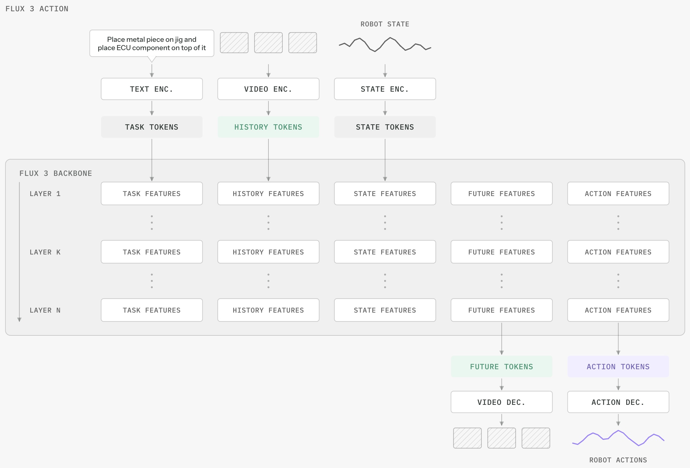
From Video Pretraining to Action Midtraining

Action midtraining introduces action-conditioned physical data after broad visual pretraining, adapting a general video representation toward controllable dynamics without discarding the visual priors learned at scale.
The central scaling hypothesis is that video supplies physical structure before expensive robot supervision is introduced. More than 95% of FLUX 3 Action’s pretraining tokens are video, with the remaining mixture primarily consisting of images and a small amount of audio. FLUX 3 Action reports that a checkpoint without this pretraining remains below 1% success in its controlled RoboLab adaptation experiment, whereas video-heavy pretraining substantially improves downstream action learning.
During action-focused midtraining, the model retains multimodal video data while introducing heterogeneous sources with aligned actions. The reported sample mixture contains 36.95% joint video/audio data, 19.55% game recordings, 13.54% egocentric video with hand-pose annotations, 14.03% handheld-gripper data, and 15.93% teleoperation data spanning 14 robot embodiments. This treats “action” more broadly than robot joint commands: game controls, human hand motion, handheld end-effectors, and robot teleoperation all provide temporally aligned evidence about how interventions change visual observations.
The training progression can therefore be summarized as:
\[\boxed{ \text{video-heavy multimodal pretraining} \rightarrow \text{heterogeneous action midtraining} \rightarrow \text{embodiment-specific post-training} }\]
Rather than expecting robot demonstrations to teach both visual dynamics and control from scratch, the video backbone supplies a prior over temporal change, while action-aligned data grounds that prior in executable control. In practice, the representation must preserve the task-relevant geometry, state, and uncertainty needed by downstream reasoning and control rather than only semantic appearance.
The following figure (source) shows RoboLab results across random initialization, multimodal-pretrained checkpoints, and action-midtrained checkpoints, highlighting the contribution of video-heavy pretraining and continued action midtraining to downstream robot-control performance.

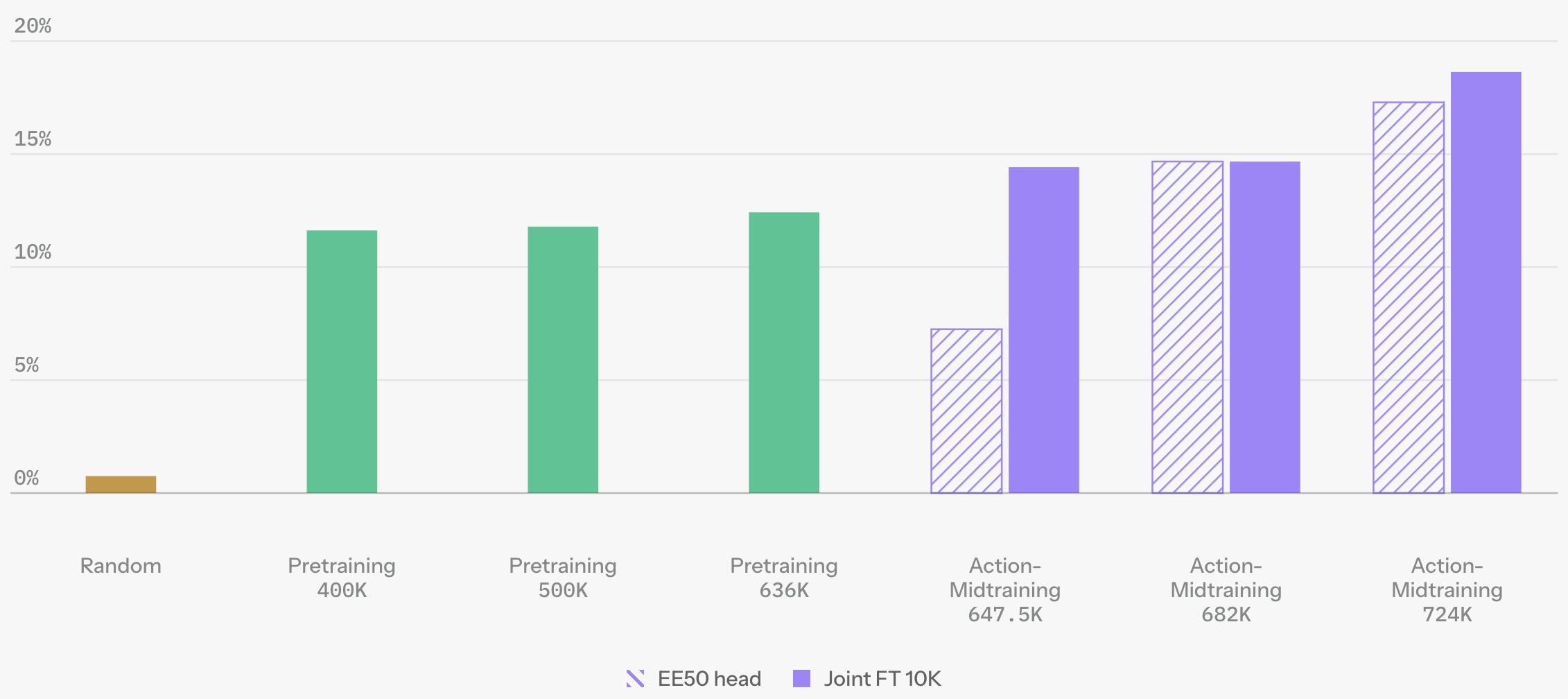
Action Representation and Embodiment Adaptation

Action Representation and Embodiment Adaptation specializes shared perceptual and semantic knowledge to the target robot by calibrating its action interface, dynamics, workspace, and control frequency with embodiment-specific experience.
FLUX 3 Action must reconcile heterogeneous embodiments whose native action spaces are incompatible. For pose-based egocentric, handheld, and teleoperation data, FLUX 3 Action describes an EE50 representation with 50 dimensions: 25 dimensions for each of two end-effectors, including translation, a 6D rotation representation, and hand-articulation or gripper channels; unused dimensions are zero-padded. Some robot datasets instead retain a 14-dimensional joint-space representation.
Embodiment-specific normalization and adaptation remain necessary even with a shared backbone:
\[z_t=f_\theta\left(I_{\leq t},g\right)\] \[\hat a_{t:t+H}^{(e)}=h_e\left(z_t,s_t^{(e)}\right)\]
- where $f_\theta$ captures broadly reusable visual-temporal structure and $h_e$ maps that structure into the action semantics of embodiment $e$. This mirrors the distinction between transferable physical knowledge and embodiment-specific actuation.
The released system demonstrates this adaptation pattern on DROID-style Franka manipulation and the low-cost SO-101 arm. The FLUX 3 Action fine-tuning guide provides DROID and SO-101 checkpoints and LeRobot integration, illustrating how a general WAM backbone can be specialized rather than retrained from scratch for each robot.
The following figure (source) shows RoboLab success across timestep distributions, distribution shifts, and action scales used for joint video-action denoising, including the high-performing logit-logistic configuration selected for subsequent training.

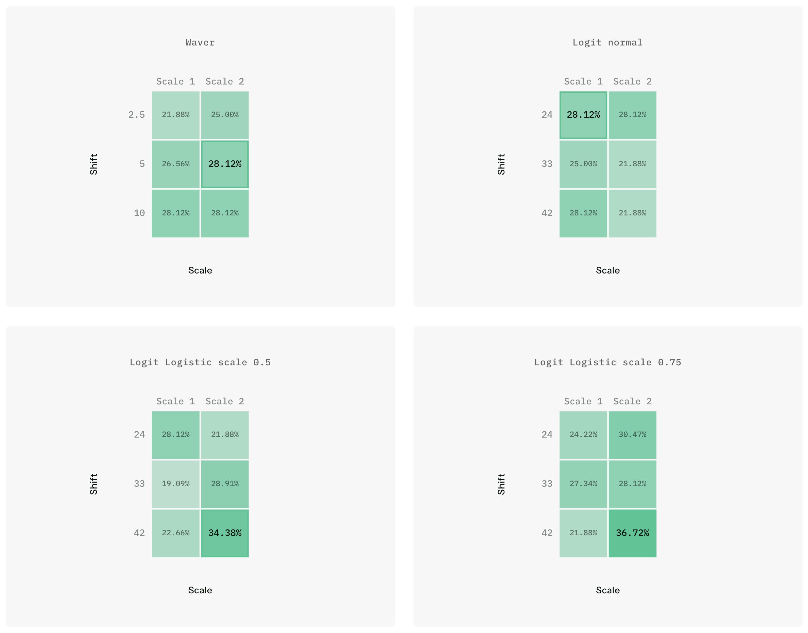
Receding-Horizon Closed-Loop Control

Receding-Horizon Closed-Loop Control alternates short-horizon action execution with fresh sensing, retaining enough commitment for smooth control while repeatedly correcting the plan as the physical state changes.
FLUX 3 Action predicts 32 actions per call at a 15 Hz control rate, corresponding to approximately 2.13 seconds of planned motion. The robot need not execute the entire chunk open-loop: it can execute a prefix, acquire a fresh observation, and invoke the model again:
\[\left(I_t,s_t,g\right) \rightarrow \hat a_{t:t+H} \rightarrow \text{execute first }K\text{ actions} \rightarrow I_{t+K},s_{t+K} \rightarrow \text{replan}\]
The replanning interval $K$ creates a direct tradeoff between responsiveness and inference cost. A larger $K$ amortizes model inference over a longer motion horizon, while a smaller $K$ incorporates environmental changes sooner. This is especially important for WAMs because joint video-action generation produces longer token sequences than action-only policies.
FLUX 3 Action reports that its fastest step-distilled variant improves real-time factor relative to $\pi_{0.5}$ largely because each call covers 2.13 seconds of robot motion rather than the 1.0-second chunk used in the comparison; this does not imply lower latency for every individual inference call. A useful systems quantity is:
\[\mathrm{RTF} = \frac{T_{\mathrm{inference}}}{T_{\mathrm{action\ chunk}}}\]
The following figure (source) shows the RoboLab success-rate versus inference-speed trade-off across FLUX 3 Action variants and competing policies, including the Pareto frontier across serving precisions and hardware settings.

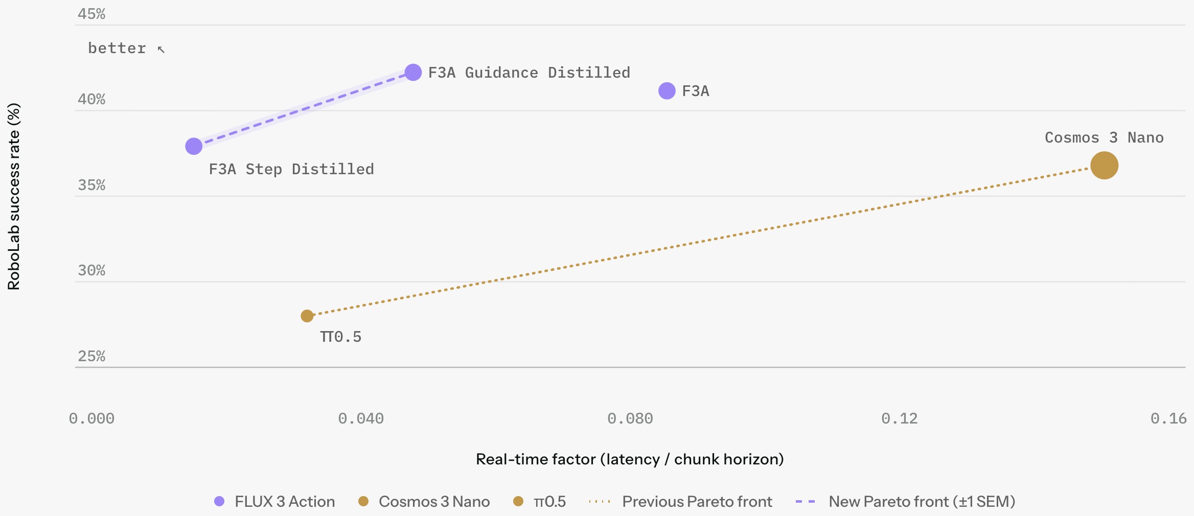
Simulation Evaluation and Real-Robot Validation

Simulation Evaluation and Real-Robot Validation models how physical state evolves under actions, enabling counterfactual prediction, planning, synthetic experience, and closed-loop evaluation before every decision is attempted in the real world.
RoboLab: A High-Fidelity Simulation Benchmark for Analysis of Task Generalist Policies by Yang et al. (2026) evaluates task-generalist robot policies on 120 manipulation tasks in Isaac Lab, with automated success detection and multiple forms of language specificity. FLUX 3 Action reported 515 successful trials out of 1,200, or 42.9%, on RoboLab-120; this placed it first on the public leaderboard at release, although the live leaderboard evolves as new policies are added.
The release-time comparison included $\pi_{0.5}$: a Vision-Language-Action Model with Open-World Generalization by Physical Intelligence et al. (2025), Cosmos 3: Omnimodal World Models for Physical AI by NVIDIA et al. (2026), and World Action Models are Zero-shot Policies by Ye et al. (2026). The broader result is evidence that video-pretrained action models can be competitive with VLA policies on simulated manipulation, not proof that WAMs universally dominate VLAs.
Simulation results must be separated from physical deployment. RoboLab is a high-fidelity simulation benchmark, so a high score measures performance under its task distribution and simulator rather than establishing equivalent robustness on real hardware. FLUX 3 Action additionally reports blind third-party Franka tests on ten single-object DROID tasks, where it completed 28 of 30 attempts. Such tests provide complementary evidence, but remain much narrower than open-world deployment.
The following figure (source) shows a physical Franka-arm rollout for the “Put the cube in the bowl” manipulation task, one of the blind DROID tasks used in the third-party real-robot evaluation.

The following figure (source) shows SO-101 rollouts under out-of-distribution object changes, illustrating object-level generalization after embodiment-specific fine-tuning.

WAMs Versus VLAs

VLAs map observations and instructions directly to actions, whereas world-action models additionally exploit predictive structure about how the scene evolves under candidate actions; the distinction is whether future-state modeling is implicit in the policy or exposed as an explicit modeling target.
WAMs and VLAs make different bets about where physical knowledge should enter the policy. A VLA can leverage strong semantic priors and learn:
\[\left(I_{\leq t},s_{\leq t},g\right)\rightarrow a_{t:t+H}\]
- whereas a WAM explicitly preserves future-world prediction:
  \[\left(I_{\leq t},s_{\leq t},g\right) \rightarrow \left(I_{t+1:t+H},a_{t:t+H}\right)\]
The WAM formulation offers a route to improved data efficiency because large-scale video can teach temporal regularities without robot action labels. World Action Models are Zero-shot Policies by Ye et al. (2026) reports that DreamZero can exploit video-only demonstrations and adapt across embodiments, while mimic-video: Video-Action Models for Generalizable Robot Control Beyond VLAs by Pai et al. (2025) reports substantial gains in sample efficiency by reusing a pretrained video backbone for control.
The cost is computational. Predicting future visual tokens in addition to actions increases sequence length and inference work, and generative policies may require multiple denoising or flow steps. FLUX 3 Action addresses this through guidance distillation, step distillation, FP8 inference, caching of prompt-dependent computation, and compilation optimizations. This makes the architectural comparison a systems tradeoff:
\[\boxed{ \text{physical prior from video} + \text{joint future prediction} \quad\leftrightarrow\quad \text{compute} + \text{latency} + \text{memory} }\]
The broader significance is that video generation and robot policy learning are becoming less separable. A temporal generative model can provide not only synthetic training data for a downstream policy, but also the representation and predictive mechanism used by the policy itself. FLUX 3 Action therefore sits between the conventional categories of “world model” and “action model”: it treats future-world prediction as part of action generation rather than as a separate simulator queried by the controller.

World Models and VLAs

World Models and VLAs models how physical state evolves under actions, enabling counterfactual prediction, planning, synthetic experience, and closed-loop evaluation before every decision is attempted in the real world.
World Models and VLAs should optimize for decision-relevant prediction: contact, geometry, timing, and task progress matter when they change which action is preferred, whereas visually conspicuous errors may be harmless if they do not affect control.
A VLA and world model solve complementary conditional prediction problems. Its usefulness therefore depends less on visual plausibility alone than on whether predicted state changes preserve the consequences that would alter a downstream decision.
The VLA predicts actions:
\[\boxed{ \text{VLA}: \quad p_\theta( a_{t:t+H} \mid o_{\leq t},g ) }\]
The world model predicts consequences:
\[\boxed{ \text{World Model}: \quad p_\phi( o_{t+1:t+H} \mid o_{\leq t},a_{t:t+H} ). }\]
Connecting them creates a closed reasoning loop:
\[\boxed{ \text{VLA proposes} \rightarrow \text{World Model predicts} \rightarrow \text{Evaluator scores} \rightarrow \text{VLA acts}. }\]
This can be interpreted as a learned version of model-predictive control. Instead of trusting the first proposed action sequence, the system can internally test candidate behaviors before executing them.
For a more extensive treatment of this relationship, including JEPA-style predictive architectures, latent dynamics, VLAs, and world-model learning, see our World Models primer. Its usefulness therefore depends less on visual plausibility alone than on whether predicted state changes preserve the consequences that would alter a downstream decision.

World Models as Critics

World Models as Critics uses predicted consequences to score candidate behavior, effectively turning the learned dynamics model into a critic over actions or plans before they are executed.
World Models as Critics should optimize for decision-relevant prediction: contact, geometry, timing, and task progress matter when they change which action is preferred, whereas visually conspicuous errors may be harmless if they do not affect control.
A world model can also support policy post-training without directly selecting actions. This is the point where learned predictions meet coordinate frames, control rates, actuator limits, and the closed-loop dynamics of the physical system.
Suppose a VLA proposes $A = a_{t:t+H}$, the world model predicts:
\[\hat\tau = M_\phi( o_{\leq t},A )\]
A critic evaluates:
\[R = C( \hat\tau )\]
The resulting signal can train the VLA:
\[\theta \leftarrow \theta + \eta \nabla_\theta J(\pi_\theta)\]
Thus,
\[\boxed{ \text{World Model} \rightarrow \text{Experience Generator} + \text{Counterfactual Evaluator} }\]
This creates a natural bridge between foundation world models and reinforcement-learning post-training. Its usefulness therefore depends less on visual plausibility alone than on whether predicted state changes preserve the consequences that would alter a downstream decision.

From Static Datasets to Interactive Data Engines

An interactive data engine uses model failures to decide what experience to collect or generate next, turning dataset construction into a feedback process rather than a one-time preprocessing step.
From Static Datasets to Interactive Data Engines should be assessed by the new behavioral coverage it contributes, especially rare states, recovery situations, and observation-action combinations that are missing from the current training distribution.
Traditional supervised learning assumes:
\[\mathcal{D} = \text{fixed}\]
Physical AI increasingly uses:
\[\mathcal{D}_{k+1} = f( \pi_k, M_k, \mathcal{E}_k )\]
- where the next training dataset depends on the current policy, world model, and evaluation results.
The dataset therefore evolves with the agent. What matters is not only the number of examples but also their coverage of tasks, embodiments, recovery states, and observation-action alignments that the deployed policy will encounter.
This is a major conceptual shift:
\[\boxed{ \text{dataset} \rightarrow \text{data engine}. }\]
World models make this possible because they can generate targeted experience on demand. Its usefulness therefore depends less on visual plausibility alone than on whether predicted state changes preserve the consequences that would alter a downstream decision.

World Models as Learned Simulators

World Models as Learned Simulators combines learned prediction with explicit or implicit physical structure so candidate actions can be tested against contact, geometry, timing, and dynamics before real execution.
World Models as Learned Simulators should vary or calibrate the physical and sensing factors that materially affect the deployed policy, with success measured by transfer to held-out real behavior rather than by simulator performance alone.
A sufficiently capable world model begins to approximate the interface of a simulator. Its usefulness therefore depends less on visual plausibility alone than on whether predicted state changes preserve the consequences that would alter a downstream decision.
A simulator exposes:
\[\operatorname{step}(s_t,a_t) \rightarrow ( s_{t+1},r_t )\]
A learned world model can approximate:
\[\operatorname{step}_\phi( z_t,a_t ) \rightarrow ( z_{t+1}, \hat r_t )\]
If observations can also be rendered $o_{t+1} = D(z_{t+1})$, the model becomes a complete learned interactive environment. In practice, the representation must preserve the task-relevant geometry, state, and uncertainty needed by downstream reasoning and control rather than only semantic appearance.
This leads toward a powerful abstraction:
\[\boxed{ \text{World Model} \approx \text{Generative Simulator} }\]

The World-Model Physical AI Stack

The World-Model Physical AI Stack matters because physical policies need a way to test counterfactual actions and observe their downstream consequences before every experiment is attempted on real hardware.
The World-Model Physical AI Stack should be evaluated through the behavior it produces after integration, because component-level metrics can miss timing, state-distribution, and control-interface failures that only appear in closed-loop execution.
The emerging stack can be summarized as:
\[\boxed{ \begin{array}{c} \text{Real-World Video + Robot Data}\\ \downarrow\\ \text{Representation Learning}\\ \downarrow\\ \text{World Foundation Model}\\ \downarrow\\ \text{Domain Post-Training}\\ \downarrow\\ \text{Interactive Simulation}\\ \downarrow\\ \text{Policy Rollouts}\\ \downarrow\\ \text{Counterfactual Evaluation}\\ \downarrow\\ \text{Policy Post-Training}\\ \downarrow\\ \text{Physical Deployment}\\ \circlearrowleft \end{array} }\]
The central idea is that a Physical AI system increasingly learns both sides of the interaction:
\[\boxed{ \underbrace{\pi_\theta}_{\text{agent}} + \underbrace{M_\phi}_{\text{world}} }\]
The policy learns how to act. The world model learns what actions do.
Together they enable an increasingly important training paradigm:
\[\boxed{ \text{observe reality} \rightarrow \text{learn a world} \rightarrow \text{imagine experience} \rightarrow \text{improve the agent} \rightarrow \text{return to reality}. }\]
The next section will examine the Physical AI Data Engine in detail, including teleoperation, robot demonstrations, Open X-Embodiment, human video, action normalization, cross-embodiment data, simulation, domain randomization, synthetic trajectories, world-model-generated experience, data mixtures, filtering, and curriculum construction.

The Physical AI Data Engine

Robot foundation models require diverse, well-structured experience, not merely more observations. This chapter traces how demonstrations, human video, simulation, and autonomous rollouts become training data.

Robot Data Fundamentals

This section develops why physical ai is a data problem in the context of the broader Physical AI system. It connects the underlying concepts to the implementation details discussed below.

Why Physical AI Is a Data Problem

Why Physical AI Is a Data Problem is governed by the distribution of physical experience available for learning: useful scale comes from covering tasks, embodiments, recovery states, and action consequences rather than simply accumulating more frames.
Why Physical AI Is a Data Problem should be assessed by the new behavioral coverage it contributes, especially rare states, recovery situations, and observation-action combinations that are missing from the current training distribution.
Physical AI is constrained not only by model capacity, but by the amount, diversity, and quality of experience available for training. Language models can learn from enormous corpora of naturally occurring text. Physical agents require observations paired with actions, state transitions, outcomes, and often task descriptions:
\[\tau = \{ (o_t,s_t,a_t,r_t) \}_{t=1}^{T}\]
Collecting such trajectories on real robots is expensive because every sample requires interaction with physical hardware. Robots operate in real time, demonstrations require operators or autonomous policies, hardware experiences wear and failure, and unsafe exploration cannot simply be scaled arbitrarily.
The central data challenge is:
\[\boxed{ \text{How can limited physical experience be transformed into sufficiently broad training experience?} }\]
Modern Physical AI systems increasingly answer this through a data engine combining real demonstrations, heterogeneous robot datasets, human video, simulation, synthetic data, world models, autonomous rollouts, and targeted failure collection. Because each executed command changes the next input distribution, the relevant unit of evaluation is the resulting rollout rather than an isolated one-step prediction.
The resulting pipeline is not a static dataset:
\[\boxed{ \text{Collect} \rightarrow \text{Train} \rightarrow \text{Evaluate} \rightarrow \text{Discover Failures} \rightarrow \text{Generate Data} \rightarrow \text{Retrain}. }\]

What Constitutes a Robot Trajectory?

What Constitutes a Robot Trajectory? must account for the fact that an autonomous vehicle changes the future scene through its own motion and through the reactions of other agents. Closed-loop evaluation is therefore essential for separating trajectories that look plausible in recorded logs from policies that remain safe and effective under interaction.
What Constitutes a Robot Trajectory? should be assessed by the new behavioral coverage it contributes, especially rare states, recovery situations, and observation-action combinations that are missing from the current training distribution.
A robot demonstration contains substantially more structure than an image-caption pair. In practice, the representation must preserve the task-relevant geometry, state, and uncertainty needed by downstream reasoning and control rather than only semantic appearance.
A trajectory may contain:
\[\tau = \{ I_t^{1:N}, D_t, q_t, \dot q_t, g_t, a_t, l, r_t \}_{t=1}^{T}\]
- where:
  - $I_t^{1:N}$ represents one or more camera streams.
  - $D_t$ represents depth or other spatial sensing.
  - $q_t$ and $\dot q_t$ represent robot joint positions and velocities.
  - $g_t$ represents gripper state.
  - $a_t$ represents the executed action.
  - $l$ represents the language instruction.
  - $r_t$ optionally represents reward or task feedback.
The training example is therefore temporally structured:
\[(o_{\leq t},l) \rightarrow a_{t:t+H}\]
For a VLA, the important supervision is not simply what appears in an image, but what action should follow from the current physical context. In practice, the representation must preserve the task-relevant geometry, state, and uncertainty needed by downstream reasoning and control rather than only semantic appearance.

Sources of Physical AI Data

Sources of Physical AI Data is governed by the distribution of physical experience available for learning: useful scale comes from covering tasks, embodiments, recovery states, and action consequences rather than simply accumulating more frames.
Sources of Physical AI Data should be assessed by the new behavioral coverage it contributes, especially rare states, recovery situations, and observation-action combinations that are missing from the current training distribution.
A modern Physical AI data mixture may be written as:
\[\mathcal{D} = \mathcal{D}_{\mathrm{robot}} + \mathcal{D}_{\mathrm{human}} + \mathcal{D}_{\mathrm{internet}} + \mathcal{D}_{\mathrm{sim}} + \mathcal{D}_{\mathrm{synthetic}} + \mathcal{D}_{\mathrm{autonomous}}\]
These sources provide different forms of supervision. Robot demonstrations provide direct action labels. Human video provides enormous visual coverage of physical interactions but usually lacks robot actions. Internet-scale image-text and video-text data provides semantic knowledge.
Simulation provides controllable state-action trajectories. Generative models can synthesize new observations and scenarios. Autonomous rollouts provide experience under the current policy’s own state distribution.
The challenge is therefore not merely collecting more data. It is combining heterogeneous data sources whose semantics, embodiments, observation spaces, and action spaces differ.

Human Demonstrations

Human Demonstrations provides dense examples of successful task structure, while embodiment mismatch means human motion usually must be retargeted or abstracted before it can supervise robot control directly.
Human Demonstrations should be assessed by the new behavioral coverage it contributes, especially rare states, recovery situations, and observation-action combinations that are missing from the current training distribution.
The most direct method for collecting robot data is to ask a human to demonstrate a task. What matters is not only the number of examples but also their coverage of tasks, embodiments, recovery states, and observation-action alignments that the deployed policy will encounter.
The following figure (source) shows ALOHA, a low-cost, open-source bimanual teleoperation system built using off-the-shelf robot arms and 3D-printed components. On the left, a human operator controls the follower robots by physically manipulating the leader robots. On the right, examples demonstrate the system’s ability to collect demonstrations for precise, contact-rich, and dynamic manipulation tasks, alongside tasks subsequently executed by learned policies.

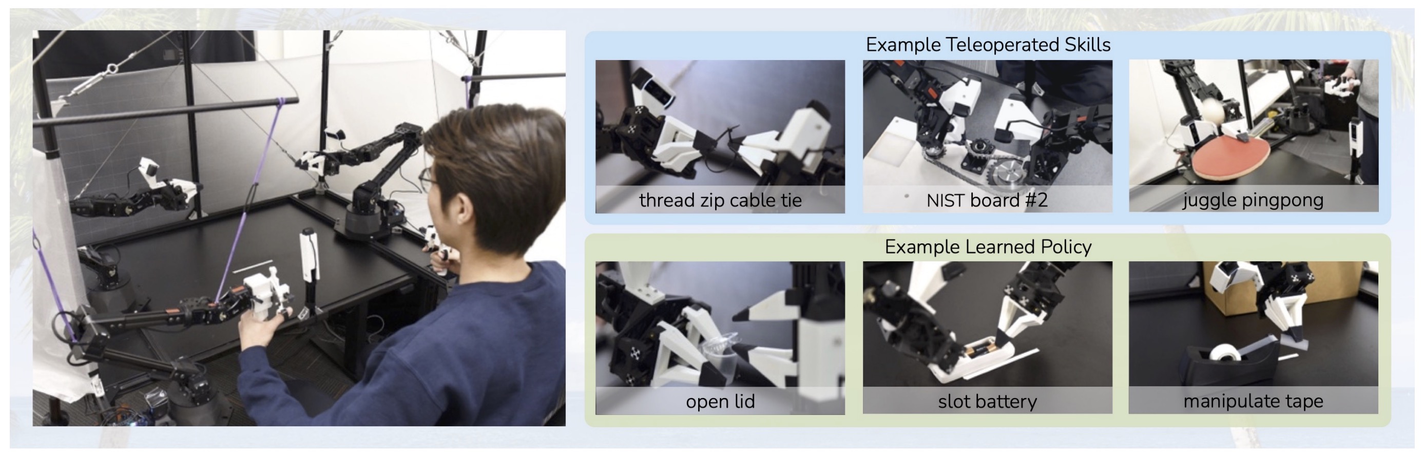
A demonstration provides:
\[\tau_E = \{ (o_t,a_t) \}_{t=1}^{T}\]
- where the subscript $E$ denotes an expert.
Behavioral cloning then learns:
\[\pi_\theta(a_t\mid o_{\leq t},l)\]
- by minimizing:
  \[\mathcal{L}_{\mathrm{BC}} = - \mathbb{E}_{(o,a)\sim\mathcal{D}_E} [ \log \pi_\theta(a\mid o,l) ]\]
Demonstrations are particularly valuable because they concentrate data around successful behavior rather than requiring the robot to discover useful actions through random exploration. This is the point where learned predictions meet coordinate frames, control rates, actuator limits, and the closed-loop dynamics of the physical system.
However, demonstration quality strongly influences the learned policy:
\[\boxed{ \text{policy quality} \lesssim \text{coverage and quality of demonstrations}. }\]

Teleoperation

Teleoperation is fundamentally a question of information value rather than raw sample count. Different sources contribute different forms of supervision, so mixture design should account for coverage, action grounding, embodiment specificity, cost, and the failure regions that remain underrepresented after training.
Teleoperation data is valuable because it records robot-native actions together with the observations that motivated them, but operator style and interface latency can become systematic biases in the training distribution.
Teleoperation allows a human to control a robot while the system records observations and actions. The operator may use devices such as joysticks, VR controllers, motion-capture systems, leader-follower robot arms, or other interfaces.
Conceptually,
\[u_t^{\mathrm{human}} \xrightarrow{f_{\mathrm{teleop}}} a_t^{\mathrm{robot}}\]
The resulting dataset contains:
\[(o_t,a_t^{\mathrm{robot}},l)\]
Teleoperation has become one of the primary mechanisms for collecting manipulation data because it produces robot-native action labels. This is the point where learned predictions meet coordinate frames, control rates, actuator limits, and the closed-loop dynamics of the physical system.
The challenge is scalability. If collecting one hour of robot experience requires approximately one hour of human operation, dataset growth remains constrained by human labor and hardware throughput.

Demonstration Quality Versus Demonstration Quantity

Demonstration Quality Versus Demonstration Quantity reflects a tradeoff between broad state coverage and precise action supervision: more demonstrations help only when their observation-action pairs are consistent enough to teach reliable behavior.
Demonstration Quality Versus Demonstration Quantity should be assessed by the new behavioral coverage it contributes, especially rare states, recovery situations, and observation-action combinations that are missing from the current training distribution.
Not all demonstrations contribute equally.
A useful dataset must balance:
\[\text{quantity}, \quad \text{quality}, \quad \text{diversity}\]
Repeating one task thousands of times can improve robustness around that task but may contribute less to generalization than collecting diverse objects, scenes, embodiments, and behaviors. What matters is not only the number of examples but also their coverage of tasks, embodiments, recovery states, and observation-action alignments that the deployed policy will encounter.
One can view dataset utility as:
\[U(\mathcal{D}) = f( N, C_{\mathrm{task}}, C_{\mathrm{object}}, C_{\mathrm{scene}}, C_{\mathrm{embodiment}}, Q )\]
- where $N$ is dataset size, $C$ terms denote different kinds of coverage, and $Q$ denotes demonstration quality.
The data-engine problem is therefore an allocation problem: determining which additional trajectories provide the greatest marginal improvement. What matters is not only the number of examples but also their coverage of tasks, embodiments, recovery states, and observation-action alignments that the deployed policy will encounter.

Language Annotation

Language annotations connect trajectories to reusable semantic concepts such as goals, object relations, and task phases, allowing one policy to share experience across demonstrations that differ at the raw action level.
Language annotation increases the reuse value of trajectories by attaching goals, subgoals, object relations, or task phases to physical experience that would otherwise be indexed only by raw sensor and action streams.
A robot trajectory becomes more useful for generalist instruction following when paired with language. A trajectory $\tau$ can be associated with instruction $l = \text{``place the red cup in the sink''}$.
Training then learns:
\[\pi_\theta(a\mid o,l)\]
Multiple linguistic descriptions can correspond to the same behavior:
\[\{ l_1,l_2,\ldots,l_K \} \leftrightarrow \tau\]
For example:
\[l_1 = \text{``put away the cup''}\] \[l_2 = \text{``move the red mug into the sink''}\]
Language augmentation can therefore increase linguistic diversity without requiring new physical trajectories. For embodied use, that semantic interpretation must remain tied to the current scene, the robot state, and the actions that are actually feasible for the embodiment.

Open X-Embodiment

Open X-Embodiment pools heterogeneous robot trajectories to learn shared structure across embodiments, while standardized observation and action interfaces make otherwise incompatible datasets jointly trainable.
Open X-Embodiment should distinguish broadly reusable semantic and perceptual representations from robot-specific calibration in kinematics, dynamics, sensing, action ranges, and recovery behavior.
One of the major developments in robot learning has been the aggregation of datasets collected across many institutions and robot platforms. Open X-Embodiment: Robotic Learning Datasets and RT-X Models by the Open X-Embodiment Collaboration et al. (2023) assembled data from 22 robot embodiments contributed by 21 institutions, producing a large cross-embodiment resource for training generalist robot policies. The central idea is that instead of learning $\pi_{\theta,e}$ for a single embodiment $e$, the model learns $\pi_\theta(a \mid o,l,e)$ across many embodiments.
The data mixture becomes:
\[\mathcal{D} = \bigcup_{e=1}^{E} \mathcal{D}_e\]
This is conceptually analogous to multilingual language modeling:
\[\text{many languages} \rightarrow \text{shared language model}\]
- while robot learning uses:
  \[\text{many embodiments} \rightarrow \text{shared physical policy}\]

Demonstrations and Cross-Embodiment Data

This section connects rt-x and positive transfer across robots with the cross-embodiment normalization problem. The discussion develops the relevant methods, implementation details, and practical tradeoffs.

RT-X and Positive Transfer Across Robots

RT-X pools trajectories across heterogeneous robots so that shared visual and task structure can transfer across embodiments, while robot-specific action conventions are normalized at the interfaces.
RT-X and Positive Transfer Across Robots must be analyzed as part of the timed execution path from observation to actuation, because stale state, wrong frames, or delayed commands can invalidate an otherwise accurate prediction.
Open X-Embodiment was used to train RT-X models that share knowledge across robot datasets. The work demonstrated that combining heterogeneous robot experience can improve performance relative to training exclusively on some individual datasets, while also exposing the difficulty of reconciling different embodiments and data distributions.
The important principle is positive transfer:
\[\mathcal{D}_A + \mathcal{D}_B \rightarrow \text{better performance on }A\]
This suggests that physical skills contain reusable structure. A useful plan therefore has to connect high-level intent to reachable intermediate states and leave room to replan when execution produces an unexpected observation.
For example,
\[\text{grasping}, \quad \text{placing}, \quad \text{pushing}, \quad \text{opening}\]
- share geometric and semantic regularities even when performed by different robots.
Cross-embodiment pretraining attempts to capture these regularities. The training stage should therefore be interpreted by the capability it is intended to add: broad representations, embodiment grounding, task adaptation, or closed-loop behavioral improvement.

The Cross-Embodiment Normalization Problem

The Cross-Embodiment Normalization Problem must reconcile robot-specific units, ranges, joint structures, and control conventions so a shared model can learn common behavior without confusing incompatible command semantics.
The Cross-Embodiment Normalization Problem must be analyzed as part of the timed execution path from observation to actuation, because stale state, wrong frames, or delayed commands can invalidate an otherwise accurate prediction.
Different robots expose different action spaces. This is the point where learned predictions meet coordinate frames, control rates, actuator limits, and the closed-loop dynamics of the physical system.
Robot $A$ may use $a_t^A \in \mathbb{R}^{7}$ while robot $B$ may use:
\[a_t^B \in \mathbb{R}^{14}\]
One robot may use Cartesian end-effector deltas:
\[a_t = [ \Delta x, \Delta y, \Delta z, \Delta r, g ]\]
- while another exposes joint-space targets:
  \[a_t = [ q_1,\ldots,q_n ]\]
Even identical quantities can have different ranges and units. Transfer is therefore easiest for semantic and perceptual structure, while action normalization, kinematics, reachable states, and safety limits still require embodiment-aware handling.
A common normalization is:
\[\tilde a_i = \frac{ a_i-\mu_i }{ \sigma_i }\]
- or percentile-based scaling such as:
  \[\tilde a_i = 2 \frac{ a_i-q_i^{0.01} }{ q_i^{0.99}-q_i^{0.01} } -1\]
At inference time,
\[a_i = f_e^{-1}( \tilde a_i )\]
- where $f_e^{-1}$ is embodiment-specific.
Normalization is not merely numerical preprocessing. It defines how heterogeneous physical control spaces are mapped into a shared policy representation.

Embodiment Metadata

Embodiment Metadata gives the policy explicit information about morphology, sensors, or action conventions, providing a conditioning signal for choosing behavior appropriate to the current robot.
Embodiment metadata makes heterogeneous trajectories interpretable to a shared policy by identifying robot morphology, sensor configuration, action conventions, and other context needed to decode each example correctly.
A generalist policy may explicitly condition on embodiment information:
\[e = \{ \text{robot type}, \text{DoF}, \text{camera configuration}, \text{action specification} \}\]
The policy becomes:
\[\pi_\theta( a \mid o,l,e )\]
Alternatively, embodiment can be inferred implicitly from observations. Explicit conditioning is useful when the same semantic instruction must map to substantially different physical actions.
For example, $\text{``pick up the cup''}$ could require different kinematics for a single-arm manipulator, dual-arm humanoid, or mobile manipulator.

Dataset Standardization

Dataset Standardization prevents representational mismatches from being mistaken for learning problems. Units, coordinate frames, action conventions, timing, padding, and embodiment metadata must remain explicit so heterogeneous examples describe comparable physical quantities.
Dataset standardization makes heterogeneous robot experience jointly trainable by aligning schemas, timestamps, coordinate conventions, task labels, and action representations before examples enter the shared mixture.
Cross-embodiment training requires a common data representation. What matters is not only the number of examples but also their coverage of tasks, embodiments, recovery states, and observation-action alignments that the deployed policy will encounter.
A standardized episode might contain:

episode/
    observations/
        camera_0
        camera_1
        proprioception
    actions/
    language/
    timestamps/
    embodiment_metadata/
    success/

At timestep $t$, the loader constructs $x_t = \{I_{t-k:t},s_{t-k:t},l,e\}$ and target $y_t = a_{t:t+H}$. The loader must also reconcile camera rates, control rates, missing modalities, action conventions, coordinate frames, and trajectory boundaries.
For large Physical AI systems, this data infrastructure can be as consequential as the policy architecture itself. This is the point where learned predictions meet coordinate frames, control rates, actuator limits, and the closed-loop dynamics of the physical system.

Temporal Alignment

Temporal alignment determines whether observations, language, proprioception, and actions describe the same physical moment; misalignment can teach a policy to associate commands with stale state or delayed consequences.
Temporal Alignment should be evaluated through the behavior it produces after integration, because component-level metrics can miss timing, state-distribution, and control-interface failures that only appear in closed-loop execution.
Sensors and controls frequently operate at different rates. Suppose cameras run at $f_{\mathrm{cam}}$ while actions are recorded at $f_{\mathrm{control}}$.
The dataset must align:
\[I(t) \leftrightarrow a(t)\]
If timestamps are inaccurate, the model may learn an artificial temporal offset:
\[I_t \rightarrow a_{t+\Delta}\]
For fast physical systems, even modest synchronization errors can materially degrade learning. Maintaining this context is important because delayed effects, partial observability, and earlier execution errors can all change which action is appropriate at the current step.
A robust data pipeline therefore preserves high-resolution timestamps and explicitly resamples modalities into a common training timeline. What matters is not only the number of examples but also their coverage of tasks, embodiments, recovery states, and observation-action alignments that the deployed policy will encounter.

Human Video as Physical Pretraining Data

Human Video as Physical Pretraining Data is fundamentally a question of information value rather than raw sample count. Different sources contribute different forms of supervision, so mixture design should account for coverage, action grounding, embodiment specificity, cost, and the failure regions that remain underrepresented after training.
Human video scales cheaply and captures rich object interactions, but it contributes indirect supervision because human motions must be abstracted or retargeted before they become robot-native action examples.
Robot data is scarce, but human video is abundant. What matters is not only the number of examples but also their coverage of tasks, embodiments, recovery states, and observation-action alignments that the deployed policy will encounter.
A human manipulation video contains useful information about:
\[\text{objects}, \quad \text{affordances}, \quad \text{contacts}, \quad \text{task structure}, \quad \text{temporal dynamics}\]
The central difficulty is that it does not directly contain robot actions:
\[I_{1:T}^{\mathrm{human}} \not\Rightarrow a_{1:T}^{\mathrm{robot}}\]
Nevertheless, video can provide representation learning, task understanding, motion priors, or latent-action supervision. In practice, the representation must preserve the task-relevant geometry, state, and uncertainty needed by downstream reasoning and control rather than only semantic appearance.
This creates an attractive scaling route:
\[\boxed{ \text{internet video} \rightarrow \text{physical representation} \rightarrow \text{robot adaptation} }\]

Learning Representations from Human Activity

Human activity video provides abundant supervision about object state, contact, and temporal structure, but transferring it to robots requires separating embodiment-independent visual knowledge from human-specific motion.
Learning Representations from Human Activity should be evaluated through the behavior it produces after integration, because component-level metrics can miss timing, state-distribution, and control-interface failures that only appear in closed-loop execution.
R3M: A Universal Visual Representation for Robot Manipulation by Nair et al. (2022) showed that representations pretrained on large-scale human video can transfer effectively to downstream robotic manipulation. Instead of learning visual features only from robot data, $f_{\mathrm{vision}} \leftarrow \mathcal{D}_{\mathrm{robot}}$ the model first learns from $\mathcal{D}_{\mathrm{human-video}}$ then adapts to $\mathcal{D}_{\mathrm{robot}}$.
This separates two problems $\boxed{\text{learning how the physical world looks}}$ from $\boxed{\text{learning how a particular robot acts}}$. The key systems implication is that model quality must ultimately be judged through executable behavior under the sensing, dynamics, and timing constraints of the physical platform.

Human Video and Representation Learning

This section connects learning latent actions from video with internet-scale semantic data. The discussion develops the relevant methods, implementation details, and practical tradeoffs.

Learning Latent Actions from Video

Latent-action learning infers compact control variables from video when explicit robot commands are unavailable, creating an intermediate behavior space that can later be grounded to a target embodiment.
Learning Latent Actions from Video is useful only if compression preserves the variables that change rewards and action rankings; high reconstruction quality is neither necessary nor sufficient for that decision-level requirement.
Human and internet video often lacks explicit actions. One strategy is to infer latent actions:
\[z_t^a = f_{\mathrm{action}} ( o_t,o_{t+1} )\]
A dynamics model then predicts:
\[\hat o_{t+1} = f_{\mathrm{dyn}} ( o_t,z_t^a )\]
The latent variable is encouraged to encode the transformation responsible for moving the environment from one observation to the next. In practice, the representation must preserve the task-relevant geometry, state, and uncertainty needed by downstream reasoning and control rather than only semantic appearance.
Later, a smaller amount of robot data can ground these latent actions into robot commands:
\[z_t^a \rightarrow a_t^{\mathrm{robot}}\]
This is attractive because it separates scalable physical-dynamics learning from expensive robot-action labeling. This is the point where learned predictions meet coordinate frames, control rates, actuator limits, and the closed-loop dynamics of the physical system.

Internet-Scale Semantic Data

Internet-scale image, video, and language data supplies broad semantic priors about objects and interactions, complementing robot data that is scarcer but necessary for grounding those concepts in executable behavior.
Internet-Scale Semantic Data should be assessed by the new behavioral coverage it contributes, especially rare states, recovery situations, and observation-action combinations that are missing from the current training distribution.
Physical agents also benefit from ordinary vision-language data. In practice, the representation must preserve the task-relevant geometry, state, and uncertainty needed by downstream reasoning and control rather than only semantic appearance.
Image-text and video-text pretraining can teach concepts such as:
\[\text{cup}, \quad \text{drawer}, \quad \text{fragile}, \quad \text{pour}, \quad \text{behind}\]
Robot data then grounds these semantic concepts in action. For embodied use, that semantic interpretation must remain tied to the current scene, the robot state, and the actions that are actually feasible for the embodiment.
The training mixture may therefore contain:
\[\mathcal{D} = \lambda_{\mathrm{VL}} \mathcal{D}_{\mathrm{VL}} + \lambda_{\mathrm{robot}} \mathcal{D}_{\mathrm{robot}}\]
This is the basic data rationale behind VLA architectures built from pretrained vision-language models. In practice, the representation must preserve the task-relevant geometry, state, and uncertainty needed by downstream reasoning and control rather than only semantic appearance.
Internet-scale data provides semantic breadth; robot data provides physical grounding. For embodied use, that semantic interpretation must remain tied to the current scene, the robot state, and the actions that are actually feasible for the embodiment.

Simulation as a Data Source

Simulation as a Data Source turns learned dynamics into a source of additional experience, allowing targeted counterfactual trajectories to supplement expensive real interaction when their fidelity is sufficient for the downstream policy.
Simulation as a Data Source should be assessed by the new behavioral coverage it contributes, especially rare states, recovery situations, and observation-action combinations that are missing from the current training distribution.
Simulation replaces expensive physical interaction with programmable experience. This is the point where learned predictions meet coordinate frames, control rates, actuator limits, and the closed-loop dynamics of the physical system.
A simulator implements:
\[s_{t+1} = F_{\mathrm{sim}} ( s_t,a_t;\phi )\]
- where $\phi$ contains environment parameters such as masses, friction coefficients, object geometry, lighting, and sensor properties.
The simulator can generate:
\[\tau_{\mathrm{sim}} = \{ (s_t,o_t,a_t,r_t) \}_{t=1}^{T}\]
Unlike real-world data collection, simulation can often be parallelized aggressively $\{E_1,E_2,\ldots,E_N\}$ can execute simultaneously. The practical question is whether the generated variation covers the geometry, dynamics, sensing, and timing errors that materially affect transfer to the real system.
This makes simulation particularly valuable for reinforcement learning, where policy improvement may require large numbers of environment interactions. This is the point where learned predictions meet coordinate frames, control rates, actuator limits, and the closed-loop dynamics of the physical system.

Domain Randomization

Domain Randomization is most useful when the simulation variables correspond to uncertainties that matter in deployment. Geometry, dynamics, sensing, latency, and actuation should therefore be calibrated or randomized deliberately, with transfer judged by held-out real behavior rather than simulation performance alone.
Domain Randomization varies deployment-sensitive parameters such as appearance, camera properties, friction, mass, latency, and actuator response so the learned policy does not depend on one narrow simulator configuration.
A policy trained in one perfectly deterministic simulator may overfit to its exact parameters. This is the point where learned predictions meet coordinate frames, control rates, actuator limits, and the closed-loop dynamics of the physical system.
Domain randomization instead samples:
\[\phi \sim p(\phi)\]
Parameters may include:
\[\phi = \{ m, \mu, k, c, L, T, \eta \}\]
- representing quantities such as mass, friction, stiffness, damping, lighting, textures, and sensor noise.
Training becomes:
\[\max_\theta \mathbb{E}_{\phi\sim p(\phi)} [ R( \pi_\theta; \phi ) ]\]
The policy therefore learns behavior robust across a family of environments rather than a single simulator configuration. This is the point where learned predictions meet coordinate frames, control rates, actuator limits, and the closed-loop dynamics of the physical system.
The intuition is:
\[\boxed{ \text{make simulation diverse enough that reality becomes another variation} }\]

Dynamics Randomization

Dynamics randomization varies masses, friction, delays, actuator response, and related physical parameters so a policy cannot overfit to one simulator configuration and is more likely to tolerate real-system uncertainty.
Dynamics Randomization should optimize for decision-relevant prediction: contact, geometry, timing, and task progress matter when they change which action is preferred, whereas visually conspicuous errors may be harmless if they do not affect control.
For control, visual randomization alone is insufficient. In practice, the representation must preserve the task-relevant geometry, state, and uncertainty needed by downstream reasoning and control rather than only semantic appearance.
Physical parameters can be randomized:
\[m \sim p(m)\] \[\mu \sim p(\mu)\] \[\tau_{\mathrm{motor}} \sim p(\tau_{\mathrm{motor}})\] \[\Delta t_{\mathrm{latency}} \sim p(\Delta t)\]
This exposes the policy to variation in mass, friction, motor strength, latency, and contact dynamics. A robust policy then learns:
\[\pi_\theta = \arg\max_\pi \mathbb{E}_{\phi} [ R(\pi;\phi) ]\]

Synthetic Visual Data

Synthetic Visual Data is fundamentally a question of information value rather than raw sample count. Different sources contribute different forms of supervision, so mixture design should account for coverage, action grounding, embodiment specificity, cost, and the failure regions that remain underrepresented after training.
Synthetic visual data can expand appearance and scene diversity without robot time, while its utility depends on whether the rendered cues that drive policy decisions transfer to real sensing.
Simulation can also generate labeled visual observations. In practice, the representation must preserve the task-relevant geometry, state, and uncertainty needed by downstream reasoning and control rather than only semantic appearance.
Because the simulator knows the full scene state, labels such as:
\[\text{depth}, \quad \text{segmentation}, \quad \text{pose}, \quad \text{optical flow}, \quad \text{contact}\]
- can be produced automatically.
If rendering function $R$ maps scene state to image,
\[I_t = R(s_t,\phi_{\mathrm{visual}})\]
- then changing visual parameters generates many appearances of the same physical trajectory.
This can improve robustness while preserving exact state-action supervision. In practice, the representation must preserve the task-relevant geometry, state, and uncertainty needed by downstream reasoning and control rather than only semantic appearance.

Procedural Environment Generation

Procedural generation expands coverage by varying layouts, objects, and task configurations under known rules, making it possible to sample structured diversity more systematically than with a fixed collection of scenes.
Procedural Environment Generation should vary or calibrate the physical and sensing factors that materially affect the deployed policy, with success measured by transfer to held-out real behavior rather than by simulator performance alone.
Simulation becomes substantially more useful when environments themselves are generated procedurally. Let $z \sim p(z)$ represent environment parameters. A generator creates $E = G(z)$.
Different samples can vary:
\[\text{room layout}, \quad \text{objects}, \quad \text{obstacles}, \quad \text{lighting}, \quad \text{task goals}\]
The policy trains over:
\[E_1,E_2,\ldots,E_N\]
Procedural generation therefore turns environmental diversity into a programmable quantity.

Synthetic Robot Demonstrations

Synthetic Robot Demonstrations expands supervision without equal real-robot cost, but synthetic actions remain useful only when their dynamics, observations, and task outcomes transfer to the deployment embodiment.
Synthetic Robot Demonstrations should be assessed by the new behavioral coverage it contributes, especially rare states, recovery situations, and observation-action combinations that are missing from the current training distribution.
Simulation can produce not only environments but demonstrations. The practical question is whether the generated variation covers the geometry, dynamics, sensing, and timing errors that materially affect transfer to the real system.
Suppose a privileged planner has access to simulator state:
\[a_t^* = \pi_{\mathrm{expert}}( s_t )\]
The training policy receives only observations:
\[o_t = O(s_t)\]
The resulting synthetic dataset is:
\[\mathcal{D}_{\mathrm{synthetic}} = \{ (o_t,a_t^*) \}\]
The policy then learns:
\[\pi_\theta( a_t \mid o_t )\]
This is privileged-information distillation:
\[\boxed{ \text{simulator-state expert} \rightarrow \text{observation-based physical policy}. }\]

Simulation and Synthetic Data

This section connects generative models as data engines with targeted data generation. The discussion develops the relevant methods, implementation details, and practical tradeoffs.

Generative Models as Data Engines

Generative models can act as data engines by producing targeted scenes, trajectories, and perturbations, but generated experience is useful only when it preserves the causal structure that the downstream policy must exploit.
Generative Models as Data Engines should be assessed by the new behavioral coverage it contributes, especially rare states, recovery situations, and observation-action combinations that are missing from the current training distribution.
Generative models add another source of synthetic data. The practical question is whether the generated variation covers the geometry, dynamics, sensing, and timing errors that materially affect transfer to the real system.
Instead of constructing every simulated scene manually,
\[E_i = \text{human-authored}\]
- a generative model can produce:
  \[E_i \sim p_\phi( E\mid c )\]
  - where $c$ describes a desired scenario.
For example,
\[c = \text{``cluttered kitchen with partially open drawers''}\]
A world model can then generate corresponding visual futures or interactive environments. In practice, the representation must preserve the task-relevant geometry, state, and uncertainty needed by downstream reasoning and control rather than only semantic appearance.
This allows the data engine to request experience rather than merely consume existing data. What matters is not only the number of examples but also their coverage of tasks, embodiments, recovery states, and observation-action alignments that the deployed policy will encounter.

Targeted Data Generation

Targeted generation is most valuable when driven by observed failure modes, because synthetic examples can then concentrate compute on underrepresented states instead of reproducing already-solved portions of the distribution.
Targeted Data Generation should be assessed by the new behavioral coverage it contributes, especially rare states, recovery situations, and observation-action combinations that are missing from the current training distribution.
Random synthetic generation is often inefficient. The practical question is whether the generated variation covers the geometry, dynamics, sensing, and timing errors that materially affect transfer to the real system.
Suppose evaluation identifies a failure distribution:
\[p_{\mathrm{fail}}(x)\]
The data generator should preferentially sample:
\[x \sim q(x)\]
- where:
  \[q(x) \propto p_{\mathrm{fail}}(x) \cdot w(x)\]
Here $w(x)$ can prioritize severity, uncertainty, or expected learning value. What matters is not only the number of examples but also their coverage of tasks, embodiments, recovery states, and observation-action alignments that the deployed policy will encounter.
The resulting loop is:
\[\boxed{ \text{Evaluate} \rightarrow \text{Cluster Failures} \rightarrow \text{Generate Similar Cases} \rightarrow \text{Train} \rightarrow \text{Re-evaluate}. }\]
This is more scalable than increasing dataset size indiscriminately. What matters is not only the number of examples but also their coverage of tasks, embodiments, recovery states, and observation-action alignments that the deployed policy will encounter.

GR00T-Dreams as a Synthetic Data Pipeline

GR00T-Dreams as a Synthetic Data Pipeline is fundamentally a question of information value rather than raw sample count. Different sources contribute different forms of supervision, so mixture design should account for coverage, action grounding, embodiment specificity, cost, and the failure regions that remain underrepresented after training.
GR00T-Dreams as a Synthetic Data Pipeline should be assessed by the new behavioral coverage it contributes, especially rare states, recovery situations, and observation-action combinations that are missing from the current training distribution.
NVIDIA’s GR00T-Dreams applies generative AI and simulation to robot-training data generation. The system uses world-generation and simulation tools to create synthetic robot experiences that can supplement limited real demonstrations.
The broader pipeline can be represented as:
\[\mathcal{D}_{\mathrm{real}} \rightarrow \text{scenario generation} \rightarrow \mathcal{D}_{\mathrm{synthetic}} \rightarrow \text{policy training}\]
The objective is to amplify scarce physical demonstrations:
\[N_{\mathrm{real}} \ll N_{\mathrm{train}}\]
- where:
  \[N_{\mathrm{train}} = N_{\mathrm{real}} + N_{\mathrm{synthetic}}\]
The synthetic data is valuable only if it preserves the task semantics and physical constraints required by the policy. For embodied use, that semantic interpretation must remain tied to the current scene, the robot state, and the actions that are actually feasible for the embodiment.

World-Model-Generated Experience

World-model rollouts can provide counterfactual experience beyond recorded trajectories, allowing policies to explore alternative actions while avoiding the cost and risk of executing every trial on real hardware.
World-Model-Generated Experience should be evaluated through the behavior it produces after integration, because component-level metrics can miss timing, state-distribution, and control-interface failures that only appear in closed-loop execution.
A world model provides another mechanism for synthetic trajectories. Its usefulness therefore depends less on visual plausibility alone than on whether predicted state changes preserve the consequences that would alter a downstream decision.
Given initial context $o_{\leq t}$ and action sequence $a_{t:t+H}$ the model generates:
\[\hat o_{t+1:t+H} \sim p_\phi( o_{t+1:t+H} \mid o_{\leq t}, a_{t:t+H} )\]
These imagined trajectories can be used for planning, policy evaluation, or training. The key advantage is that world-model generation can be conditioned on the current policy’s weaknesses. For example,
\[c = \text{``generate scenarios where this grasp fails because the object slips''}\]
The resulting experience can directly target failure modes.

Autonomous Data Collection

Autonomous collection closes the data loop by letting deployed agents identify uncertain or failed situations and contribute new trajectories, making coverage evolve with the policy rather than remain fixed.
Autonomous Data Collection should be assessed by the new behavioral coverage it contributes, especially rare states, recovery situations, and observation-action combinations that are missing from the current training distribution.
Once a policy becomes sufficiently capable, it can collect its own data. Instead of $a_t = a_t^{\mathrm{human}}$, the robot executes $a_t \sim \pi_\theta(a_t\mid o_t)$.
The resulting trajectories expose the policy’s actual state distribution:
\[s_t \sim d^{\pi_\theta}(s)\]
This is important because behavioral cloning trains primarily on $s_t \sim d^{\pi_E}(s)$ the expert distribution. What matters is not only the number of examples but also their coverage of tasks, embodiments, recovery states, and observation-action alignments that the deployed policy will encounter.
Autonomous rollouts reveal states caused by the learner’s own errors. Because each executed command changes the next input distribution, the relevant unit of evaluation is the resulting rollout rather than an isolated one-step prediction.

Human Intervention and Corrections

Human interventions provide high-value corrective examples near failure states, supplying supervision exactly where pure behavioral cloning often has the least support.
Human Intervention and Corrections should report the task distribution, trial protocol, failure criteria, and interaction budget explicitly so improvements can be attributed to capability rather than easier scenarios or hidden assistance.
Pure autonomous collection can be unsafe or produce low-quality data. A human can intervene when the policy begins to fail.
Suppose:
\[a_t^{\mathrm{policy}} = \pi_\theta(o_t)\]
When intervention trigger $I_t=1$,
\[a_t = a_t^{\mathrm{human}}\]
The correction provides particularly valuable supervision because it occurs near the policy’s failure boundary. In practice, the representation must preserve the task-relevant geometry, state, and uncertainty needed by downstream reasoning and control rather than only semantic appearance.
The resulting dataset contains
\[(o_t,a_t^{\mathrm{human}})\]
- precisely where $\pi_\theta(o_t)$ was inadequate.
This is a powerful form of active data collection. What matters is not only the number of examples but also their coverage of tasks, embodiments, recovery states, and observation-action alignments that the deployed policy will encounter.

DAgger and On-Policy Demonstration Collection

DAgger and On-Policy Demonstration Collection addresses distribution shift by collecting expert labels on states visited by the current policy, moving the training distribution toward the situations the learned controller will actually encounter.
DAgger and On-Policy Demonstration Collection should be assessed by the new behavioral coverage it contributes, especially rare states, recovery situations, and observation-action combinations that are missing from the current training distribution.
A Reduction of Imitation Learning and Structured Prediction to No-Regret Online Learning by Ross et al. (2011) introduced DAgger, which iteratively collects expert labels on states visited by the learner rather than training only on a fixed expert trajectory distribution.
The procedure is approximately:
\[\pi_k \rightarrow \text{rollout} \rightarrow s\sim d^{\pi_k} \rightarrow a^*=\pi_E(s) \rightarrow \mathcal{D}_{k+1}\]
The dataset grows as:
\[\mathcal{D}_{k+1} = \mathcal{D}_k \cup \{ (s,a^*) \}\]
This directly addresses covariate shift by training the policy on states it actually visits. This is the point where learned predictions meet coordinate frames, control rates, actuator limits, and the closed-loop dynamics of the physical system.
Modern robot data engines generalize this idea through autonomous rollouts, interventions, corrections, failure mining, and targeted recollection. This is the point where learned predictions meet coordinate frames, control rates, actuator limits, and the closed-loop dynamics of the physical system.

Success and Failure Data

Success and Failure Data is informative only when the evaluation distribution, success criteria, intervention policy, and trial protocol are explicit. Aggregate scores should be paired with failure categories and scenario coverage so improvements are not caused by easier task mixes or hidden changes in evaluation conditions.
Success-only datasets teach nominal behavior but provide little evidence about recovery; retaining failed and corrected trajectories gives the learner examples of the states that matter most once execution drifts off demonstration.
Early imitation-learning datasets often emphasize successful demonstrations. But failures contain important information.
A successful trajectory tells the model:
\[\text{what works}\]
A failed trajectory can reveal:
\[\text{what does not work and why}\]
Suppose the dataset contains outcome:
\[y_\tau \in \{ 0,1 \}\]
A value or success model can learn:
\[V_\psi(\tau) = P( y_\tau=1 \mid \tau )\]
Failures can then support reward learning, critic training, preference learning, and RL post-training. What matters is not only the number of examples but also their coverage of tasks, embodiments, recovery states, and observation-action alignments that the deployed policy will encounter.
The data engine should therefore preserve failure trajectories rather than discarding them automatically. What matters is not only the number of examples but also their coverage of tasks, embodiments, recovery states, and observation-action alignments that the deployed policy will encounter.

Autonomous Collection and Data Quality

This section connects automatic success detection with data filtering. The discussion develops the relevant methods, implementation details, and practical tradeoffs.

Automatic Success Detection

Automatic Success Detection is informative only when the evaluation distribution, success criteria, intervention policy, and trial protocol are explicit. Aggregate scores should be paired with failure categories and scenario coverage so improvements are not caused by easier task mixes or hidden changes in evaluation conditions.
Automatic Success Detection should be evaluated through the behavior it produces after integration, because component-level metrics can miss timing, state-distribution, and control-interface failures that only appear in closed-loop execution.
Scaling robot data collection requires automatic labeling of whether tasks succeeded. What matters is not only the number of examples but also their coverage of tasks, embodiments, recovery states, and observation-action alignments that the deployed policy will encounter.
A success classifier estimates
\[p_\psi( y=1 \mid o_{1:T},l )\]
This classifier may use final images, video, robot state, task metadata, or multimodal foundation models. In practice, the representation must preserve the task-relevant geometry, state, and uncertainty needed by downstream reasoning and control rather than only semantic appearance.
For instruction
\[l = \text{``put the apple in the bowl''}\]
- the evaluator determines whether the final state satisfies the instruction.
Automatic success detection enables large-scale autonomous rollouts because human reviewers no longer need to label every trajectory. This is the point where learned predictions meet coordinate frames, control rates, actuator limits, and the closed-loop dynamics of the physical system.
However, evaluator errors become part of the training signal, so success models themselves require careful calibration. The training stage should therefore be interpreted by the capability it is intended to add: broad representations, embodiment grounding, task adaptation, or closed-loop behavioral improvement.

Data Filtering

Filtering removes corrupted, low-quality, irrelevant, or inconsistent trajectories before training so model capacity is spent on examples whose observations and actions form a trustworthy learning signal.
Data Filtering should be assessed by the new behavioral coverage it contributes, especially rare states, recovery situations, and observation-action combinations that are missing from the current training distribution.
More data is not always better.
A raw trajectory corpus may contain
\[\text{failed teleoperation}, \quad \text{sensor corruption}, \quad \text{idle periods}, \quad \text{incorrect labels}, \quad \text{duplicate trajectories}\]
Define quality score
\[q_i = Q(\tau_i)\]
Training data can be filtered using
\[\mathcal{D}' = \{ \tau_i \mid q_i>\delta \}\]
Alternatively, examples can be weighted:
\[\mathcal{L} = \sum_i w_i \mathcal{L}(\tau_i)\]
- where
  \[w_i=f(q_i)\]
Filtering becomes increasingly important as synthetic and autonomous data expand dataset scale. The practical question is whether the generated variation covers the geometry, dynamics, sensing, and timing errors that materially affect transfer to the real system.

Deduplication

Deduplication reduces repeated near-identical trajectories that would otherwise distort the effective training distribution and make nominal dataset scale overstate behavioral diversity.
Deduplication should be assessed by the new behavioral coverage it contributes, especially rare states, recovery situations, and observation-action combinations that are missing from the current training distribution.
Repeated trajectories can distort the effective training distribution. The training stage should therefore be interpreted by the capability it is intended to add: broad representations, embodiment grounding, task adaptation, or closed-loop behavioral improvement.
If trajectory $\tau_i$ appears many times,
\[p_{\mathrm{train}}(\tau_i)\]
- becomes artificially large.
Exact duplicate detection is straightforward, but semantic duplication is harder. Two trajectories may be visually different while encoding nearly identical behavior.
Embedding-based similarity can estimate
\[d( f(\tau_i), f(\tau_j) ) < \epsilon\]
Near-duplicate clusters can then be downsampled.
The objective is not maximum raw dataset size but maximum useful diversity. What matters is not only the number of examples but also their coverage of tasks, embodiments, recovery states, and observation-action alignments that the deployed policy will encounter.

Data Balancing

Balancing adjusts the relative frequency of tasks, embodiments, outcomes, and state regimes so common behaviors do not dominate gradients at the expense of rare but important capabilities.
Data Balancing should be assessed by the new behavioral coverage it contributes, especially rare states, recovery situations, and observation-action combinations that are missing from the current training distribution.
Suppose the dataset contains
\[90\% \text{pick-and-place}\]
- and
  \[1\% \text{drawer opening}\]
Naive sampling trains primarily on the dominant task. What matters is not only the number of examples but also their coverage of tasks, embodiments, recovery states, and observation-action alignments that the deployed policy will encounter.
Instead, define task sampling distribution
\[p_{\mathrm{train}}(k) \propto w_kN_k^\alpha\]
- where $N_k$ is the number of examples for task $k$ and
  
  $0\leq\alpha\leq1$ controls how strongly raw frequency determines
  - sampling.
When
\[\alpha=1\]
- sampling follows the raw dataset.
When
\[\alpha=0\]
- tasks are sampled uniformly.
Intermediate values trade off diversity and statistical efficiency. What matters is not only the number of examples but also their coverage of tasks, embodiments, recovery states, and observation-action alignments that the deployed policy will encounter.

Mixing Data Sources

Mixing web, simulation, human, and robot data requires explicit sampling weights because each source has different scale, fidelity, action supervision, and relevance to deployment.
Mixing Data Sources should be assessed by the new behavioral coverage it contributes, especially rare states, recovery situations, and observation-action combinations that are missing from the current training distribution.
Suppose training uses robot data, simulation, human video, and vision-language data.
The objective can be written as
\[\mathcal{L} = \lambda_R \mathcal{L}_{\mathrm{robot}} + \lambda_S \mathcal{L}_{\mathrm{sim}} + \lambda_H \mathcal{L}_{\mathrm{human}} + \lambda_V \mathcal{L}_{\mathrm{VL}}\]
The coefficients
\[\lambda_R,\lambda_S,\lambda_H,\lambda_V\]
- determine the effective training curriculum.
These weights may change during training.
Early training can emphasize broad semantic and physical representation learning:
\[\lambda_H,\lambda_V \uparrow\]
Later training can emphasize robot-native actions:
\[\lambda_R \uparrow\]
Post-training may emphasize high-quality or task-specific trajectories. What matters is not only the number of examples but also their coverage of tasks, embodiments, recovery states, and observation-action alignments that the deployed policy will encounter.

Curriculum Learning

Curriculum learning orders or reweights experience so the policy acquires prerequisite behaviors before harder compositions, which can improve optimization when difficult tasks are otherwise too sparse or unstable.
Curriculum Learning should be assessed by the new behavioral coverage it contributes, especially rare states, recovery situations, and observation-action combinations that are missing from the current training distribution.
Not all physical tasks should necessarily be introduced with equal probability from the beginning.
A curriculum can progress from
\[\text{simple} \rightarrow \text{complex}\]
For manipulation:
\[\text{reach} \rightarrow \text{grasp} \rightarrow \text{place} \rightarrow \text{multi-object manipulation} \rightarrow \text{long-horizon task}\]
More generally, training distribution at step $k$ is
\[p_k(\tau)\]
- and the curriculum updates it:
  \[p_{k+1}(\tau) = f( p_k, \text{performance}_k )\]
Tasks the policy already masters can be downweighted while difficult but learnable tasks receive more sampling probability. This is the point where learned predictions meet coordinate frames, control rates, actuator limits, and the closed-loop dynamics of the physical system.

Automatic Curriculum Generation

Automatic curriculum generation uses learning progress or failure signals to choose the next tasks, turning task selection itself into an adaptive component of the training system.
Automatic Curriculum Generation should be assessed by the new behavioral coverage it contributes, especially rare states, recovery situations, and observation-action combinations that are missing from the current training distribution.
A stronger data engine uses evaluation results to construct the curriculum automatically. What matters is not only the number of examples but also their coverage of tasks, embodiments, recovery states, and observation-action alignments that the deployed policy will encounter.
Suppose task $i$ has success rate
\[s_i\]
A simple difficulty weight is
\[w_i = 1-s_i\]
But sampling only the hardest tasks may be inefficient if they are currently impossible.
One can instead prioritize tasks near the learning frontier:
\[w_i = f( s_i, \Delta s_i, u_i )\]
- where $\Delta s_i$ measures learning progress and $u_i$ represents uncertainty.
This yields an adaptive curriculum concentrated around tasks where additional experience is likely to improve the policy. This is the point where learned predictions meet coordinate frames, control rates, actuator limits, and the closed-loop dynamics of the physical system.

Data Mixtures and the Learning Flywheel

This section connects diversity across tasks, objects, and scenes with measuring dataset coverage. The discussion develops the relevant methods, implementation details, and practical tradeoffs.

Diversity Across Tasks, Objects, and Scenes

Dataset diversity should be measured across task, object, scene, embodiment, and behavior dimensions because raw trajectory count can grow without increasing the situations a policy can actually handle.
Diversity Across Tasks, Objects, and Scenes must be analyzed as part of the timed execution path from observation to actuation, because stale state, wrong frames, or delayed commands can invalidate an otherwise accurate prediction.
Physical generalization is multidimensional.
A useful data engine should cover the Cartesian product
\[\mathcal{G} = \mathcal{T} \times \mathcal{O} \times \mathcal{S} \times \mathcal{E} \times \mathcal{L}\]
- where:
  \[\mathcal{T} = \text{tasks}\] \[\mathcal{O} = \text{objects}\] \[\mathcal{S} = \text{scenes}\] \[\mathcal{E} = \text{embodiments}\]
  - and
    \[\mathcal{L} = \text{language}\]
The number of possible combinations grows approximately as
\[|\mathcal{G}| = |\mathcal{T}| |\mathcal{O}| |\mathcal{S}| |\mathcal{E}| |\mathcal{L}|\]
It is impossible to collect every combination physically.
Generalization therefore requires strategically sampling this space while relying on compositional transfer. The stronger test is whether the learned representation and policy continue to work when several factors shift together rather than when only one superficial attribute changes.

Measuring Dataset Coverage

Coverage metrics should expose which combinations of tasks, objects, scenes, embodiments, and recovery states are represented, making gaps visible before they appear as deployment failures.
Measuring Dataset Coverage should be assessed by the new behavioral coverage it contributes, especially rare states, recovery situations, and observation-action combinations that are missing from the current training distribution.
Dataset scale alone is an incomplete statistic. Suppose dataset $A$ contains one million trajectories from ten tasks while dataset $B$ contains 500,000 trajectories spanning one thousand tasks. Which is more useful depends on the target.
Coverage can be represented over feature space $z$:
\[z_i = f(\tau_i)\]
One can estimate density
\[p_{\mathcal{D}}(z)\]
- and identify sparse regions:
  \[p_{\mathcal{D}}(z) < \epsilon\]
These regions become candidates for targeted data collection. What matters is not only the number of examples but also their coverage of tasks, embodiments, recovery states, and observation-action alignments that the deployed policy will encounter.
Thus the data engine can explicitly optimize coverage rather than raw count. What matters is not only the number of examples but also their coverage of tasks, embodiments, recovery states, and observation-action alignments that the deployed policy will encounter.

Active Data Collection

Active collection prioritizes examples expected to reduce uncertainty or address known failures, improving the marginal value of expensive robot interaction compared with uniform data gathering.
Active Data Collection should be assessed by the new behavioral coverage it contributes, especially rare states, recovery situations, and observation-action combinations that are missing from the current training distribution.
Suppose candidate trajectory $x$ has estimated uncertainty
\[U(x)\]
The system can prioritize
\[x^* = \arg\max_x U(x)\]
More generally, data value may combine uncertainty, novelty, task importance, and failure severity:
\[V_{\mathrm{data}}(x) = \alpha U(x) + \beta N(x) + \gamma I(x) + \delta F(x)\]
The collection system then seeks
\[x^* = \arg\max_x V_{\mathrm{data}}(x)\]
This turns robot data acquisition into an active-learning problem. What matters is not only the number of examples but also their coverage of tasks, embodiments, recovery states, and observation-action alignments that the deployed policy will encounter.

Hard-Negative Mining

Hard-negative mining concentrates training on visually or semantically similar situations that require different actions, sharpening the distinctions most likely to cause consequential control errors.
Hard-Negative Mining should be assessed by the new behavioral coverage it contributes, especially rare states, recovery situations, and observation-action combinations that are missing from the current training distribution.
Policies often fail on examples close to the decision boundary. Suppose the model succeeds when objects are clearly separated but fails when distractors are visually similar.
Rather than collecting more random scenes, the data engine generates hard negatives:
\[x_{\mathrm{hard}} \sim p( x \mid \text{near policy failure boundary} )\]
For language grounding, examples might vary only a critical attribute:
\[\text{red cup} \leftrightarrow \text{orange cup}\]
For manipulation, they might vary grasp geometry slightly. The key systems implication is that model quality must ultimately be judged through executable behavior under the sensing, dynamics, and timing constraints of the physical platform.
Hard-negative mining increases the information density of additional data. What matters is not only the number of examples but also their coverage of tasks, embodiments, recovery states, and observation-action alignments that the deployed policy will encounter.

Failure Clustering

Clustering failures by mechanism can reveal recurring data gaps such as occlusion, unusual geometry, recovery states, or timing errors, which in turn provides a concrete target for the next collection cycle.
Failure Clustering should be evaluated through the behavior it produces after integration, because component-level metrics can miss timing, state-distribution, and control-interface failures that only appear in closed-loop execution.
Large-scale autonomous rollouts can produce millions of failures. Reviewing each individually is inefficient.
Embed each failure:
\[z_i = f_{\mathrm{failure}}( \tau_i )\]
Cluster
\[\{ z_1,\ldots,z_N \} \rightarrow \{ C_1,\ldots,C_K \}\]
Clusters may correspond to failure families such as
\[\text{grasp slip}, \quad \text{occlusion}, \quad \text{wrong object}, \quad \text{collision}, \quad \text{planning dead-end}\]
The data engine can then prioritize high-frequency or high-severity clusters. What matters is not only the number of examples but also their coverage of tasks, embodiments, recovery states, and observation-action alignments that the deployed policy will encounter.
This changes evaluation from a scalar success rate into an actionable data-generation system. This is the point where learned predictions meet coordinate frames, control rates, actuator limits, and the closed-loop dynamics of the physical system.

The Data Flywheel

The Data Flywheel is fundamentally a question of information value rather than raw sample count. Different sources contribute different forms of supervision, so mixture design should account for coverage, action grounding, embodiment specificity, cost, and the failure regions that remain underrepresented after training.
The Data Flywheel should be assessed by the new behavioral coverage it contributes, especially rare states, recovery situations, and observation-action combinations that are missing from the current training distribution.
The most important property of a mature Physical AI system is that deployment generates the information required for improvement. What matters is not only the number of examples but also their coverage of tasks, embodiments, recovery states, and observation-action alignments that the deployed policy will encounter.
Let policy version $k$ be
\[\pi_k\]
Deployment generates trajectories:
\[\mathcal{R}_k = \operatorname{Rollout}( \pi_k )\]
Evaluation identifies failures:
\[\mathcal{F}_k = \operatorname{Evaluate}( \mathcal{R}_k )\]
The data engine creates targeted training data:
\[\Delta\mathcal{D}_k = G( \mathcal{F}_k )\]
Training produces
\[\pi_{k+1} = \operatorname{Train}( \pi_k, \mathcal{D}_k \cup \Delta\mathcal{D}_k )\]
Then:
\[\boxed{ \pi_k \rightarrow \mathcal{R}_k \rightarrow \mathcal{F}_k \rightarrow \Delta\mathcal{D}_k \rightarrow \pi_{k+1}. }\]
This is the Physical AI data flywheel.

Data Engines Versus Datasets

A data engine differs from a static dataset because evaluation and deployment outcomes continuously influence what is collected, generated, filtered, and replayed in subsequent training rounds.
Data Engines Versus Datasets should be assessed by the new behavioral coverage it contributes, especially rare states, recovery situations, and observation-action combinations that are missing from the current training distribution.
A dataset is static:
\[\mathcal{D} = \text{constant}\]
A data engine is adaptive:
\[\mathcal{D}_{k+1} = f( \mathcal{D}_k, \pi_k, E_k )\]
- where $E_k$ represents evaluation results.
The distinction is fundamental.
A static dataset asks:
\[\text{How much data do we have?}\]
A data engine asks:
\[\text{What data should we collect next?}\]
For Physical AI, the second question increasingly determines the rate of progress. What matters is not only the number of examples but also their coverage of tasks, embodiments, recovery states, and observation-action alignments that the deployed policy will encounter.

The Emerging Physical AI Data Stack

The Emerging Physical AI Data Stack is governed by the distribution of physical experience available for learning: useful scale comes from covering tasks, embodiments, recovery states, and action consequences rather than simply accumulating more frames.
The Emerging Physical AI Data Stack should be assessed by the new behavioral coverage it contributes, especially rare states, recovery situations, and observation-action combinations that are missing from the current training distribution.
A mature Physical AI data system increasingly resembles:
\[\boxed{ \begin{array}{c} \text{Internet Images + Video}\\ +\\ \text{Human Demonstrations}\\ +\\ \text{Cross-Embodiment Robot Data}\\ +\\ \text{Simulation}\\ +\\ \text{Generative Synthetic Data}\\ +\\ \text{World-Model Rollouts}\\ +\\ \text{Autonomous Robot Experience}\\ \downarrow\\ \text{Standardization + Synchronization}\\ \downarrow\\ \text{Filtering + Deduplication}\\ \downarrow\\ \text{Normalization + Relabeling}\\ \downarrow\\ \text{Mixture Construction}\\ \downarrow\\ \text{Foundation Policy Training}\\ \downarrow\\ \text{Evaluation + Failure Mining}\\ \downarrow\\ \text{Targeted Data Generation}\\ \circlearrowleft \end{array} }\]
The broader transition is
\[\text{manual dataset collection} \rightarrow \text{automated data flywheel}\] \[\text{single-robot data} \rightarrow \text{cross-embodiment data}\] \[\text{real-only experience} \rightarrow \text{real + simulated + generated experience}\]
- and
  \[\text{random data growth} \rightarrow \text{failure-directed data acquisition}\]
Ultimately, scaling Physical AI requires scaling useful experience rather than merely scaling parameters:
\[\boxed{ \text{Physical AI capability} \approx f( \text{model scale}, \text{experience scale}, \text{experience diversity}, \text{feedback quality} ). }\]
The next section will examine Training and Post-Training Physical AI Models, including foundation-model pretraining, VLA supervised fine-tuning, behavioral cloning, offline and online reinforcement learning, reward construction, closed-loop RL, synthetic-data post-training, distillation, and the transition from broad pretrained models to deployment-ready physical policies.

Training and Post-Training

Physical AI training combines broad pretraining with embodiment-specific adaptation and task-level optimization. The sections below examine supervision, reinforcement learning, rewards, robustness, and deployment.

Training Pipeline

This section develops from foundation model to physical policy in the context of the broader Physical AI system. It connects the underlying concepts to the implementation details discussed below.

From Foundation Model to Physical Policy

From Foundation Model to Physical Policy defines which parts of perception, reasoning, and control share a pretrained representation and which remain specialized, a boundary that governs transfer, latency, interpretability, and embodiment adaptation.
From Foundation Model to Physical Policy should distinguish broadly reusable semantic and perceptual representations from robot-specific calibration in kinematics, dynamics, sensing, action ranges, and recovery behavior.
A modern Physical AI model is rarely trained for one downstream robot task from scratch. The emerging recipe is closer to the foundation-model pipeline used for language and multimodal models:
\[\boxed{ \text{Broad Pretraining} \rightarrow \text{Robot Pretraining} \rightarrow \text{Supervised Post-Training} \rightarrow \text{RL Post-Training} \rightarrow \\ \text{Deployment Adaptation} }\]
The purpose of each stage is different. Broad pretraining supplies semantic and visual knowledge. Robot pretraining grounds that knowledge in physical interaction. Supervised post-training adapts the policy to particular embodiments and tasks. Reinforcement learning improves behavior according to outcomes rather than demonstrations alone. Deployment adaptation closes remaining gaps involving latency, robustness, hardware dynamics, and the real operating distribution.
This distinction is increasingly important because a foundation policy is not necessarily a deployment-ready policy. For example, GR00T N1.5 is pretrained on a heterogeneous mixture and then post-trained on embodiment- and task-specific datasets, while Fine-Tuning Vision-Language-Action Models: Optimizing Speed and Success by Kim et al. (2025) shows that adaptation choices such as continuous actions, action chunking, and parallel decoding can materially change the performance of an already pretrained VLA.
FLUX 3 Action provides a concrete variant of this hierarchy in which physical-policy training is separated into video-heavy pretraining, heterogeneous action midtraining, and embodiment-specific post-training. FLUX 3 Action reports a pretraining mixture containing more than 95% video tokens before action-aligned data are introduced.
\[\boxed{ \text{Video-Heavy Multimodal Pretraining} \rightarrow \text{Heterogeneous Action Midtraining} \rightarrow \\ \text{Embodiment-Specific Post-Training} }\]
The middle stage is important because action capability need not be introduced only through robot demonstrations. Game controls, egocentric hand motion, handheld-gripper trajectories, and teleoperated robots provide different forms of temporally aligned action supervision, after which robot-specific input/output mappings specialize the shared model to a target embodiment. The FLUX 3 Action fine-tuning guide demonstrates this specialization for DROID-style Franka data and the low-cost SO-101 arm.
This pipeline differs from a conventional VLA recipe in one additional respect: the pretrained temporal generator continues to predict future video alongside actions. The model therefore carries its learned dynamics prior into post-training rather than using video pretraining only to initialize a perceptual encoder.

The Physical AI Training Hierarchy

The Physical AI Training Hierarchy closes the development loop by using deployment or simulation outcomes to determine what data to collect, what models to update, and which failures require another round of training.
The Physical AI Training Hierarchy should distinguish broadly reusable semantic and perceptual representations from robot-specific calibration in kinematics, dynamics, sensing, action ranges, and recovery behavior.
The training process can be viewed as progressively narrowing the model’s distribution. A useful plan therefore has to connect high-level intent to reachable intermediate states and leave room to replan when execution produces an unexpected observation.
Let the initial foundation model be
\[\theta_0\]
Broad pretraining produces
\[\theta_{\mathrm{foundation}} = \operatorname{Train} ( \theta_0, \mathcal{D}_{\mathrm{broad}} )\]
Robot pretraining then gives
\[\theta_{\mathrm{robot}} = \operatorname{Train} ( \theta_{\mathrm{foundation}}, \mathcal{D}_{\mathrm{robot}} )\]
Task-specific supervised post-training produces
\[\theta_{\mathrm{SFT}} = \operatorname{Train} ( \theta_{\mathrm{robot}}, \mathcal{D}_{\mathrm{target}} )\]
Finally, outcome-based optimization produces
\[\theta_{\mathrm{RL}} = \operatorname{RL} ( \theta_{\mathrm{SFT}}, R )\]
The progression can therefore be interpreted as
\[\boxed{ \text{knowledge} \rightarrow \text{physical grounding} \rightarrow \text{task competence} \rightarrow \text{behavioral optimization}. }\]

Broad Multimodal Pretraining

Broad multimodal pretraining supplies semantic and perceptual structure before expensive robot-specific learning, allowing downstream data to focus more directly on grounding and control.
Broad Multimodal Pretraining should connect semantic intent to the current physical state and available actions, with execution feedback used to verify that the chosen interpretation actually produced the intended effect.
Many VLAs inherit their visual and linguistic representations from pretrained VLMs. In practice, the representation must preserve the task-relevant geometry, state, and uncertainty needed by downstream reasoning and control rather than only semantic appearance.
Suppose a multimodal model learns
\[p_\theta( y \mid I,l )\]
- where $I$ represents images and $l$ represents language.
This stage can teach concepts such as
\[\text{objects}, \quad \text{attributes}, \quad \text{spatial relations}, \quad \text{instructions}, \quad \text{semantic associations}\]
But it does not yet teach the model what motor command should follow. This is the point where learned predictions meet coordinate frames, control rates, actuator limits, and the closed-loop dynamics of the physical system.
Robot training adds the physical mapping
\[(I,l,s) \rightarrow a\]
This division explains why VLAs can inherit semantic generalization from large VLMs while requiring comparatively smaller quantities of expensive action-labeled robot data. In practice, the representation must preserve the task-relevant geometry, state, and uncertainty needed by downstream reasoning and control rather than only semantic appearance.

Robot Foundation-Model Pretraining

Robot foundation-model pretraining aggregates many tasks and embodiments into a shared policy so common perceptual and behavioral structure can be reused before task- or robot-specific post-training.
Robot Foundation-Model Pretraining should distinguish broadly reusable semantic and perceptual representations from robot-specific calibration in kinematics, dynamics, sensing, action ranges, and recovery behavior.
Robot pretraining broadens the policy across tasks, environments, and embodiments before specialization. This is the point where learned predictions meet coordinate frames, control rates, actuator limits, and the closed-loop dynamics of the physical system.
The dataset can be represented as
\[\mathcal{D}_{\mathrm{pre}} = \bigcup_{e=1}^{E} \bigcup_{k=1}^{K} \mathcal{D}_{e,k}\]
- where $e$ indexes embodiments and $k$ indexes tasks or datasets.
The policy learns
\[\pi_\theta( a_{t:t+H} \mid o_{\leq t}, s_{\leq t}, l, e )\]
Open X-Embodiment: Robotic Learning Datasets and RT-X Models by the Open X-Embodiment Collaboration et al. (2023) established the importance of large cross-embodiment mixtures for generalist robot learning, while RDT-1B: a Diffusion Foundation Model for Bimanual Manipulation by Liu et al. (2024) uses heterogeneous multi-robot data and a physically interpretable unified action representation to pretrain a large diffusion-based manipulation model.
The objective is not necessarily to master every downstream task during pretraining. Instead, pretraining should create an initialization from which new physical capabilities can be acquired efficiently.

Pretraining Versus Post-Training

Pretraining Versus Post-Training is where a broad foundation policy is aligned with the target robot, task distribution, and deployment constraints. The adaptation procedure must decide which shared representations should remain stable and which components must change to capture embodiment-specific dynamics, action conventions, and failure modes.
Pretraining Versus Post-Training depends on the feedback channel available during adaptation: offline supervision favors conservative updates within known data, whereas interactive feedback can correct new failure states at the cost of additional exploration and safety management.
The boundary between pretraining and post-training is operational rather than mathematical. The training stage should therefore be interpreted by the capability it is intended to add: broad representations, embodiment grounding, task adaptation, or closed-loop behavioral improvement.
Pretraining generally optimizes broad coverage:
\[\mathcal{D}_{\mathrm{pre}} = \text{large + heterogeneous}\]
Post-training generally optimizes target behavior:
\[\mathcal{D}_{\mathrm{post}} = \text{smaller + targeted}\]
Thus,
\[\boxed{ \text{pretraining learns transferable priors;}\, \text{post-training converts them into reliable behavior} }\]
A robot foundation model may know how cups, drawers, tables, and grippers interact but still require post-training to operate a particular robot arm reliably. The training stage should therefore be interpreted by the capability it is intended to add: broad representations, embodiment grounding, task adaptation, or closed-loop behavioral improvement.

Supervised Fine-Tuning

Supervised Fine-Tuning is where a broad foundation policy is aligned with the target robot, task distribution, and deployment constraints. The adaptation procedure must decide which shared representations should remain stable and which components must change to capture embodiment-specific dynamics, action conventions, and failure modes.
Supervised Fine-Tuning depends on the feedback channel available during adaptation: offline supervision favors conservative updates within known data, whereas interactive feedback can correct new failure states at the cost of additional exploration and safety management.
The simplest post-training stage is supervised fine-tuning on demonstrations. What matters is not only the number of examples but also their coverage of tasks, embodiments, recovery states, and observation-action alignments that the deployed policy will encounter.
Given $\mathcal{D}_{\mathrm{SFT}} = \{(o_i,l_i,a_i)\}_{i=1}^{N}$, an autoregressive action policy minimizes:
\[\mathcal{L}_{\mathrm{SFT}} = - \sum_i \log \pi_\theta( a_i \mid o_i,l_i )\]
For continuous regression:
\[\mathcal{L}_{\mathrm{SFT}} = \mathbb{E} [ \| a-\hat a_\theta \|_1 ]\]
- or:
  \[\mathcal{L}_{\mathrm{SFT}} = \mathbb{E} [ \| a-\hat a_\theta \|_2^2 ]\]
For diffusion or flow-based policies, the supervised target is instead a denoising or vector-field objective. The training stage should therefore be interpreted by the capability it is intended to add: broad representations, embodiment grounding, task adaptation, or closed-loop behavioral improvement.
Regardless of parameterization, the underlying signal remains:
\[\boxed{ \text{imitate demonstrated behavior} }\]

Fine-Tuning Action Tokens

Fine-Tuning Action Tokens determines how continuous control trajectories are represented inside a sequence model. Discretization can reuse language-model machinery, but token granularity, sequence length, temporal compression, and reconstruction error directly affect both optimization and the fidelity of executed motion.
Fine-Tuning Action Tokens changes how the policy represents and executes motion, so the chosen temporal horizon and action parameterization must remain compatible with controller rate, embodiment limits, and opportunities for feedback correction.
An autoregressive VLA can quantize continuous actions into tokens. This is the point where learned predictions meet coordinate frames, control rates, actuator limits, and the closed-loop dynamics of the physical system.
For action dimension $a_i$,
\[q_i = Q(a_i) \in \{ 1,\ldots,B \}\]
The model predicts:
\[p_\theta( q_i \mid o,l,q_{<i} )\]
Training uses cross-entropy:
\[\mathcal{L}_{\mathrm{token}} = - \sum_i \log p_\theta( q_i^* \mid o,l,q_{<i}^* )\]
This approach allows an existing language-model decoder to produce actions using essentially the same mechanism used for text. For embodied use, that semantic interpretation must remain tied to the current scene, the robot state, and the actions that are actually feasible for the embodiment.
However, sequentially generating many action tokens can create unnecessary inference latency for high-frequency control. This is the point where learned predictions meet coordinate frames, control rates, actuator limits, and the closed-loop dynamics of the physical system.

Continuous-Action Fine-Tuning

Continuous-Action Fine-Tuning is where a broad foundation policy is aligned with the target robot, task distribution, and deployment constraints. The adaptation procedure must decide which shared representations should remain stable and which components must change to capture embodiment-specific dynamics, action conventions, and failure modes.
Continuous-Action Fine-Tuning depends on the feedback channel available during adaptation: offline supervision favors conservative updates within known data, whereas interactive feedback can correct new failure states at the cost of additional exploration and safety management.
An alternative is to attach a continuous action head. This is the point where learned predictions meet coordinate frames, control rates, actuator limits, and the closed-loop dynamics of the physical system.
The VLM produces hidden representation $h = f_{\mathrm{VLM}}(I,l)$ and an action head predicts:
\[\hat A = f_{\mathrm{action}}( h,s )\]
The output may be an entire action chunk:
\[\hat A = [ \hat a_t, \ldots, \hat a_{t+H-1} ]\]
Fine-Tuning Vision-Language-Action Models: Optimizing Speed and Success by Kim et al. (2025) develops the OpenVLA-OFT recipe around parallel decoding, action chunking, continuous action representations, and an L1 regression objective; the paper reports both substantially higher action-generation throughput and improved downstream performance compared with the original OpenVLA fine-tuning setup.
This illustrates an important principle:
\[\boxed{ \text{post-training architecture} \text{ can matter as much as } \text{pretrained representation quality} }\]

Supervised and Embodiment-Specific Fine-Tuning

This section connects action chunking during post-training with fine-tuning flow-matching policies. The discussion develops the relevant methods, implementation details, and practical tradeoffs.

Action Chunking During Post-Training

Action Chunking During Post-Training changes the temporal unit optimized during adaptation, letting the policy learn coherent short trajectories while preserving periodic opportunities to correct against fresh observations.
Action Chunking During Post-Training changes how the policy represents and executes motion, so the chosen temporal horizon and action parameterization must remain compatible with controller rate, embodiment limits, and opportunities for feedback correction.
Rather than predict only $a_t$, the model predicts:
\[A_t = [ a_t, a_{t+1}, \ldots, a_{t+H-1} ]\]
This provides temporal coherence and amortizes expensive foundation-model inference over multiple control steps. This is the point where learned predictions meet coordinate frames, control rates, actuator limits, and the closed-loop dynamics of the physical system.
The supervised objective becomes:
\[\mathcal{L}_{\mathrm{chunk}} = \sum_{k=0}^{H-1} \ell( \hat a_{t+k}, a_{t+k} )\]
At deployment, the system can execute the full chunk or only its first

$K$ actions:
\[K\leq H\]
Executing fewer actions before replanning increases feedback responsiveness, while executing longer chunks reduces inference cost. A useful plan therefore has to connect high-level intent to reachable intermediate states and leave room to replan when execution produces an unexpected observation.

Fine-Tuning Flow-Matching Policies

Fine-Tuning Flow-Matching Policies is where a broad foundation policy is aligned with the target robot, task distribution, and deployment constraints. The adaptation procedure must decide which shared representations should remain stable and which components must change to capture embodiment-specific dynamics, action conventions, and failure modes.
Fine-Tuning Flow-Matching Policies depends on the feedback channel available during adaptation: offline supervision favors conservative updates within known data, whereas interactive feedback can correct new failure states at the cost of additional exploration and safety management.
For models such as $\pi_0$ and $\pi_0$.5, continuous actions can be generated through flow matching. This is the point where learned predictions meet coordinate frames, control rates, actuator limits, and the closed-loop dynamics of the physical system.
Let clean action chunk be $A_1$ and noise be $A_0 \sim \mathcal{N}(0,I)$, interpolate:
\[A_\tau = (1-\tau)A_0 + \tau A_1\]
The target velocity is:
\[u_\tau = A_1-A_0\]
The model learns:
\[v_\theta( A_\tau, \tau, c ) \approx u_\tau\]
- with:
  \[\mathcal{L}_{\mathrm{FM}} = \mathbb{E} \left[ \| v_\theta(A_\tau,\tau,c) - u_\tau \|_2^2 \right]\]
Here $c$ contains visual observations, language, proprioception, and other conditioning information. In practice, the representation must preserve the task-relevant geometry, state, and uncertainty needed by downstream reasoning and control rather than only semantic appearance.
At inference, actions are generated by integrating
\[\frac{dA_\tau}{d\tau} = v_\theta( A_\tau,\tau,c )\]
- $\pi_0$.5 additionally emphasizes heterogeneous co-training across robot data, semantic prediction, web data, and other multimodal examples to improve open-world generalization.

Which Parameters Should Be Fine-Tuned?

Which Parameters Should Be Fine-Tuned? is where a broad foundation policy is aligned with the target robot, task distribution, and deployment constraints. The adaptation procedure must decide which shared representations should remain stable and which components must change to capture embodiment-specific dynamics, action conventions, and failure modes.
Which Parameters Should Be Fine-Tuned? depends on the feedback channel available during adaptation: offline supervision favors conservative updates within known data, whereas interactive feedback can correct new failure states at the cost of additional exploration and safety management.
A VLA may contain
\[\theta = \{ \theta_{\mathrm{vision}}, \theta_{\mathrm{language}}, \theta_{\mathrm{fusion}}, \theta_{\mathrm{action}} \}\]
Several adaptation strategies are possible.
Full fine-tuning updates
\[\nabla_\theta \mathcal{L}\]
- for all parameters.
Partial fine-tuning may freeze the backbone:
\[\nabla_{\theta_{\mathrm{VLM}}} \mathcal{L} = 0\]
- while updating
  \[\theta_{\mathrm{action}}\]
Parameter-efficient adaptation may update low-rank adapters or other small trainable modules. The correct choice depends on the domain shift. If semantics and visual perception transfer well but robot dynamics change, updating the action pathway may be sufficient. If the new environment introduces unfamiliar visual concepts, broader adaptation may be required.
NVIDIA reports that GR00T N1.5 freezes its VLM during both pretraining and fine-tuning while training the policy components around it, illustrating one practical decomposition between semantic representation and action learning. For embodied use, that semantic interpretation must remain tied to the current scene, the robot state, and the actions that are actually feasible for the embodiment.

Post-Training a New Embodiment

Post-Training a New Embodiment specializes shared perceptual and semantic knowledge to the target robot by calibrating its action interface, dynamics, workspace, and control frequency with embodiment-specific experience.
Post-Training a New Embodiment needs feedback that separates semantic competence from embodiment mismatch so updates focus on the target robot’s action calibration, dynamics, and control interface.
Suppose foundation policy $\pi_{\theta_0}$ was pretrained across several robots. A new robot has embodiment $e_{\mathrm{new}}$.
Collect a relatively small adaptation dataset:
\[\mathcal{D}_{\mathrm{new}} = \{ (o_i,a_i,l_i) \}_{i=1}^{N}\]
Post-training gives:
\[\theta^* = \arg\min_\theta \mathcal{L} ( \theta; \mathcal{D}_{\mathrm{new}} )\]
The intended benefit of foundation pretraining is:
\[N_{\mathrm{foundation\rightarrow new}} \ll N_{\mathrm{scratch\rightarrow new}}\]
GR00T N1.5 demonstrates this pattern through post-training on Unitree G1 teleoperation data, while its data-limited experiments also evaluate adaptation using small demonstration sets. What matters is not only the number of examples but also their coverage of tasks, embodiments, recovery states, and observation-action alignments that the deployed policy will encounter.

Post-Training for New Skills

Post-Training for New Skills is where a broad foundation policy is aligned with the target robot, task distribution, and deployment constraints. The adaptation procedure must decide which shared representations should remain stable and which components must change to capture embodiment-specific dynamics, action conventions, and failure modes.
Post-Training for New Skills depends on the feedback channel available during adaptation: offline supervision favors conservative updates within known data, whereas interactive feedback can correct new failure states at the cost of additional exploration and safety management.
Embodiment adaptation and skill adaptation are distinct. A useful plan therefore has to connect high-level intent to reachable intermediate states and leave room to replan when execution produces an unexpected observation.
The robot may already understand its own morphology but lack task
\[T_{\mathrm{new}}\]
The simplest solution is collect demonstrations:
\[\mathcal{D}_{T_{\mathrm{new}}}\]
- and continue supervised training.
Synthetic trajectories can also be used. GR00T N1.5 incorporates DreamGen-generated neural trajectories into its broader training pipeline and reports learning behaviors for which no corresponding teleoperation demonstrations were collected.
Thus skill acquisition can increasingly follow
\[\boxed{ \text{Describe Skill} \rightarrow \text{Generate Experience} \rightarrow \text{Post-Train Policy}. }\]

Why Behavioral Cloning Eventually Saturates

Why Behavioral Cloning Eventually Saturates follows from covariate shift: a policy trained only on expert states eventually encounters its own off-trajectory states, where supervised demonstrations provide progressively weaker guidance.
Behavioral cloning should therefore be evaluated beyond one-step imitation error, with particular attention to how errors compound when the learned policy controls its own future state distribution.
Behavioral cloning optimizes agreement with demonstrations:
\[\pi_\theta \approx \pi_E\]
But this imposes several limitations. First, the policy cannot systematically outperform the behavior represented in the demonstrations under the same objective.
Second, demonstrations provide sparse information about alternatives. They tell the policy:
\[\text{do this}\]
- but generally not:
  \[\text{this alternative is slightly worse}\]
  - or:
    \[\text{this action causes failure three seconds later}\]
Third, behavioral cloning primarily sees expert states:
\[s \sim d^{\pi_E}\]
- while deployment produces:
  \[s \sim d^{\pi_\theta}\]
These distributions diverge when the policy makes mistakes. This is the point where learned predictions meet coordinate frames, control rates, actuator limits, and the closed-loop dynamics of the physical system.
Outcome-based post-training addresses these limitations. The training stage should therefore be interpreted by the capability it is intended to add: broad representations, embodiment grounding, task adaptation, or closed-loop behavioral improvement.

From Imitation to Reinforcement Learning

From Imitation to Reinforcement Learning combines the stable initialization of demonstrations with interactive optimization, allowing the policy to refine behavior in states that were missing or rare in the offline dataset.
From Imitation to Reinforcement Learning depends on the feedback channel available during adaptation: offline supervision favors conservative updates within known data, whereas interactive feedback can correct new failure states at the cost of additional exploration and safety management.
Reinforcement learning optimizes expected return:
\[J(\theta) = \mathbb{E}_{\tau\sim\pi_\theta} \left[ \sum_{t=0}^{T} \gamma^t r_t \right]\]
The crucial difference is the source of supervision. In practice, the representation must preserve the task-relevant geometry, state, and uncertainty needed by downstream reasoning and control rather than only semantic appearance.
Imitation learning uses:
\[\boxed{ \text{What did the expert do?} }\]
RL uses:
\[\boxed{ \text{What happened when the policy acted?} }\]
This distinction is particularly valuable in Physical AI because many important properties are naturally outcome-based:
\[\text{task success}, \quad \text{collision}, \quad \text{object damage}, \quad \text{energy}, \quad \text{comfort}, \quad \text{time}\]

Reinforcement-Learning Post-Training

This section develops offline rl post-training in the context of the broader Physical AI system. It connects the underlying concepts to the implementation details discussed below.

Offline RL Post-Training

Offline RL Post-Training is where a broad foundation policy is aligned with the target robot, task distribution, and deployment constraints. The adaptation procedure must decide which shared representations should remain stable and which components must change to capture embodiment-specific dynamics, action conventions, and failure modes.
Offline RL Post-Training is constrained by the support of the logged dataset, so optimization must improve decisions without assigning unwarranted value to actions that were rarely or never observed.
Real robot interaction is expensive, so a natural intermediate stage is offline RL. This is the point where learned predictions meet coordinate frames, control rates, actuator limits, and the closed-loop dynamics of the physical system.
Given fixed dataset:
\[\mathcal{D} = \{ (s_t,a_t,r_t,s_{t+1}) \}\]
- the goal is to improve the policy without additional environment interaction.
A critic learns:
\[Q_\phi(s_t,a_t) \approx r_t + \gamma V(s_{t+1})\]
The policy can then favor high-value demonstrated actions:
\[\pi_\theta \leftarrow \operatorname{Improve}( Q_\phi, \mathcal{D} )\]
The central difficulty is extrapolation. If the learned policy selects actions outside the dataset distribution, the critic may assign unreliable values.
This motivates conservative algorithms such as Conservative Q-Learning for Offline Reinforcement Learning by Kumar et al. (2020) and in-distribution methods such as Offline Reinforcement Learning with Implicit Q-Learning by Kostrikov et al. (2021).

Advantage-Weighted Post-Training

Advantage-Weighted Post-Training uses reward or value information to distinguish better and worse actions without requiring unrestricted online exploration. Its reliability depends on how far policy improvement moves beyond the support of the logged data, because value estimates become less trustworthy for actions or states that were rarely observed.
Advantage-Weighted Post-Training is constrained by the support of the logged dataset, so optimization must improve decisions without assigning unwarranted value to actions that were rarely or never observed.
One useful bridge between imitation and RL is to reweight demonstrations according to estimated advantage. What matters is not only the number of examples but also their coverage of tasks, embodiments, recovery states, and observation-action alignments that the deployed policy will encounter.
Define:
\[A(s,a) = Q(s,a)-V(s)\]
Then optimize:
\[\mathcal{L}_{\mathrm{AW}} = - \mathbb{E}_{(s,a)\sim\mathcal{D}} \left[ w(s,a) \log \pi_\theta(a\mid s) \right]\]
- where:
  \[w(s,a) = \exp \left( \frac{A(s,a)}{\beta} \right)\]
High-value demonstrated actions receive more weight. This is the point where learned predictions meet coordinate frames, control rates, actuator limits, and the closed-loop dynamics of the physical system.
This is attractive for large physical policies because the final update resembles supervised learning even though the weights come from reinforcement-learning estimates. The training stage should therefore be interpreted by the capability it is intended to add: broad representations, embodiment grounding, task adaptation, or closed-loop behavioral improvement.

Online RL Post-Training

Online RL Post-Training is where a broad foundation policy is aligned with the target robot, task distribution, and deployment constraints. The adaptation procedure must decide which shared representations should remain stable and which components must change to capture embodiment-specific dynamics, action conventions, and failure modes.
Online RL Post-Training can discover useful behavior outside the offline dataset because the policy collects new experience, but exploration cost and safety become part of the learning problem.
Online RL allows the policy to execute actions, observe consequences, and update using new experience. This is the point where learned predictions meet coordinate frames, control rates, actuator limits, and the closed-loop dynamics of the physical system.
At iteration $k$:
\[\tau_k \sim \pi_{\theta_k}\]
- then:
  \[R_k = R(\tau_k)\]
  - followed by:
    \[\theta_{k+1} = \operatorname{RLUpdate}( \theta_k, \tau_k, R_k )\]
The loop is:
\[\boxed{ \text{Act} \rightarrow \text{Observe Outcome} \rightarrow \text{Update} \rightarrow \text{Act Again} }\]
This solves a fundamental weakness of offline learning: the training distribution evolves with the policy. This is the point where learned predictions meet coordinate frames, control rates, actuator limits, and the closed-loop dynamics of the physical system.
But real-world online RL can be expensive and unsafe, motivating simulation-heavy or hybrid post-training. The practical question is whether the generated variation covers the geometry, dynamics, sensing, and timing errors that materially affect transfer to the real system.

RL Post-Training for VLAs

Reinforcement-learning post-training exposes a VLA to the consequences of its own actions, allowing optimization to target task completion, recovery, and closed-loop robustness rather than imitation accuracy alone.
RL Post-Training for VLAs depends on the feedback channel available during adaptation: offline supervision favors conservative updates within known data, whereas interactive feedback can correct new failure states at the cost of additional exploration and safety management.
The same foundation-model principle used in language-model RL post-training can be applied to VLAs. For embodied use, that semantic interpretation must remain tied to the current scene, the robot state, and the actions that are actually feasible for the embodiment.
Start with a pretrained physical policy:
\[\pi_{\theta_0}\]
Generate rollouts:
\[\tau_i \sim \pi_{\theta_0}\]
Score them:
\[R_i = R( \tau_i )\]
Then optimize:
\[\theta^* = \arg\max_\theta \mathbb{E}_{\tau\sim\pi_\theta} [ R(\tau) ]\]
Recent work such as RobustVLA: Robustness-Aware Reinforcement Post-Training for Vision-Language-Action Models by Zhang et al. (2025) explicitly studies online RL post-training of pretrained VLAs and augments reward optimization with regularization for observation and action perturbations.
The broader pattern is that pretraining supplies competence while RL targets behavioral properties that demonstration likelihood alone does not directly optimize. What matters is not only the number of examples but also their coverage of tasks, embodiments, recovery states, and observation-action alignments that the deployed policy will encounter.

Reward Construction

Reward construction determines which aspects of physical behavior reinforcement learning will amplify, so progress, safety, efficiency, and completion signals must be aligned with the behavior actually desired.
Reward Construction depends on the feedback channel available during adaptation: offline supervision favors conservative updates within known data, whereas interactive feedback can correct new failure states at the cost of additional exploration and safety management.
Physical RL requires converting desired behavior into a reward. The central distinction is the source of feedback and whether the learner can safely collect new trajectories, since that determines both the optimization objective and the distribution of states available for improvement.
A generic reward may be:
\[R = w_sR_{\mathrm{success}} + w_pR_{\mathrm{progress}} + w_cR_{\mathrm{collision}} + w_mR_{\mathrm{motion}} + w_eR_{\mathrm{efficiency}}\]
For manipulation:
\[R_{\mathrm{success}} = \mathbb{1}[ \text{task completed} ]\]
A collision penalty might be:
\[R_{\mathrm{collision}} = - \sum_t \mathbb{1}[ \text{unsafe contact}_t ]\]
Smoothness may be encouraged using:
\[R_{\mathrm{motion}} = - \sum_t \| a_t-a_{t-1} \|_2^2\]
The difficulty is that reward design changes the behavior being optimized. The central distinction is the source of feedback and whether the learner can safely collect new trajectories, since that determines both the optimization objective and the distribution of states available for improvement.
Therefore:
\[\boxed{ \text{reward specification} \approx \text{behavior specification} }\]

Sparse Rewards

Sparse rewards provide a clean success signal but weak credit assignment over long horizons, making exploration and intermediate progress estimation major bottlenecks.
Sparse rewards cleanly encode completion but make credit assignment difficult, especially when many physical decisions separate the initial state from the final success signal.
The cleanest reward is often task success:
\[R(\tau) = \begin{cases} 1 & \text{task succeeds}\\ 0 & \text{otherwise} \end{cases}\]
Sparse rewards avoid encoding unwanted intermediate strategies. However, they provide little learning signal when success is rare.
If $P_{\pi}(\text{success}) \approx 0$, almost every rollout receives identical reward.
A strong pretrained policy changes this regime. If supervised pretraining already provides nontrivial success probability, RL can refine behavior from meaningful successful and failed rollouts.
This is one reason $\boxed{\text{SFT} \rightarrow \text{RL}}$ is generally more practical than learning complex physical behavior from random initialization.

Dense Rewards

Dense rewards improve credit assignment by scoring intermediate progress, but poorly chosen shaping terms can redirect the policy toward proxies that are easier to optimize than the intended task.
Dense rewards provide more frequent learning signal, but each shaping term creates another proxy the policy can exploit if it diverges from the actual task objective.
Dense rewards provide intermediate feedback.
For a reaching task:
\[r_t = - \| p_t^{\mathrm{gripper}} - p^{\mathrm{target}} \|_2\]
For object lifting:
\[r_t = \alpha r_{\mathrm{reach}} + \beta r_{\mathrm{grasp}} + \gamma r_{\mathrm{lift}}\]
Dense rewards improve exploration but can create reward hacking. For example, optimizing distance to an object does not necessarily imply a stable grasp.
Therefore, dense shaping is often combined with sparse terminal success. The central distinction is the source of feedback and whether the learner can safely collect new trajectories, since that determines both the optimization objective and the distribution of states available for improvement.

Learned Reward Models

Learned reward models can encode preferences or complex success criteria that are difficult to hand-write, but their own generalization errors become part of the reinforcement-learning objective.
Learned Reward Models replaces hand-written scoring with a learned estimate, which broadens what can be optimized but also transfers the reward model’s blind spots into the policy objective.
Some physical objectives are difficult to encode manually. The training stage should therefore be interpreted by the capability it is intended to add: broad representations, embodiment grounding, task adaptation, or closed-loop behavioral improvement.
A learned reward model can estimate:
\[R_\psi( \tau,l )\]
Training data might contain preference comparisons:
\[\tau_A \succ \tau_B\]
A Bradley-Terry-style preference model uses:
\[P( \tau_A\succ\tau_B ) = \frac{ \exp(R_\psi(\tau_A)) }{ \exp(R_\psi(\tau_A)) + \exp(R_\psi(\tau_B)) }\]
The reward model can then score new policy rollouts. This is the point where learned predictions meet coordinate frames, control rates, actuator limits, and the closed-loop dynamics of the physical system.
Multimodal foundation models also make it possible to evaluate task completion from images or videos using semantic criteria rather than manually engineered state predicates. In practice, the representation must preserve the task-relevant geometry, state, and uncertainty needed by downstream reasoning and control rather than only semantic appearance.

Reward Modeling

This section connects success models as rewards with reinforcement learning in simulation. The discussion develops the relevant methods, implementation details, and practical tradeoffs.

Success Models as Rewards

Success Models as Rewards is informative only when the evaluation distribution, success criteria, intervention policy, and trial protocol are explicit. Aggregate scores should be paired with failure categories and scenario coverage so improvements are not caused by easier task mixes or hidden changes in evaluation conditions.
Success Models as Rewards replaces hand-written scoring with a learned estimate, which broadens what can be optimized but also transfers the reward model’s blind spots into the policy objective.
For many robot tasks, the simplest learned reward is a success classifier:
\[V_\psi( o_{1:T},l ) = P( \text{success} \mid o_{1:T},l )\]
The policy reward becomes:
\[R(\tau) = V_\psi( \tau,l )\]
This makes reward construction scalable across tasks expressed in language. However, the policy can exploit errors in the success model.
Thus, $\boxed{\text{reward-model robustness}}$ becomes part of the safety problem.

Reinforcement Learning in Simulation

Reinforcement Learning in Simulation supports reinforcement learning by producing imagined or simulated experience in which policies can explore consequences more cheaply than on hardware, subject to the risk of exploiting model errors.
Reinforcement Learning in Simulation should vary or calibrate the physical and sensing factors that materially affect the deployed policy, with success measured by transfer to held-out real behavior rather than by simulator performance alone.
Simulation provides a safer environment for online exploration. The practical question is whether the generated variation covers the geometry, dynamics, sensing, and timing errors that materially affect transfer to the real system.
The policy interacts with:
\[s_{t+1} = F_{\mathrm{sim}}( s_t,a_t )\]
- instead of the physical robot.
Many environments can run concurrently:
\[E_1,E_2,\ldots,E_N\]
The total experience throughput becomes approximately:
\[R_{\mathrm{experience}} \propto N f_{\mathrm{sim}}\]
- where $f_{\mathrm{sim}}$ is the effective simulation rate.
This is especially important for humanoid locomotion, dexterous manipulation, and autonomous driving, where RL may require far more interaction than can reasonably be collected on hardware. For embodied use, that semantic interpretation must remain tied to the current scene, the robot state, and the actions that are actually feasible for the embodiment.

Sim-to-Real RL Post-Training

Sim-to-Real RL Post-Training is where a broad foundation policy is aligned with the target robot, task distribution, and deployment constraints. The adaptation procedure must decide which shared representations should remain stable and which components must change to capture embodiment-specific dynamics, action conventions, and failure modes.
Sim-to-Real RL Post-Training should vary or calibrate the physical and sensing factors that materially affect the deployed policy, with success measured by transfer to held-out real behavior rather than by simulator performance alone.
A practical pipeline is:
\[\boxed{ \text{SFT on Real Data} \rightarrow \text{RL in Simulation} \rightarrow \text{Real-World Validation} \rightarrow \text{Limited Real RL} }\]
Simulation teaches outcome-sensitive behavior at scale. Real-world data then corrects simulation mismatch.
The challenge is that:
\[P_{\mathrm{sim}} \neq P_{\mathrm{real}}\]
Domain randomization attempts to reduce this gap by optimizing:
\[J(\theta) = \mathbb{E}_{\phi\sim p(\phi)} [ R( \pi_\theta; \phi ) ]\]
The resulting policy is trained across a distribution of physical parameters rather than a single simulated world. This is the point where learned predictions meet coordinate frames, control rates, actuator limits, and the closed-loop dynamics of the physical system.

World Models for RL Post-Training

World Models for RL Post-Training supports reinforcement learning by producing imagined or simulated experience in which policies can explore consequences more cheaply than on hardware, subject to the risk of exploiting model errors.
World Models for RL Post-Training should optimize for decision-relevant prediction: contact, geometry, timing, and task progress matter when they change which action is preferred, whereas visually conspicuous errors may be harmless if they do not affect control.
A learned world model can replace or complement a conventional simulator. Its usefulness therefore depends less on visual plausibility alone than on whether predicted state changes preserve the consequences that would alter a downstream decision.
Given current state representation $z_t$ and action sequence $A$:
\[\hat\tau = M_\phi( z_t,A )\]
The policy can train against imagined experience:
\[\tau \sim M_\phi( \pi_\theta )\]
This creates:
\[\boxed{ \text{VLA} \rightarrow \text{World-Model Rollout} \rightarrow \text{Reward} \rightarrow \text{RL Update}. }\]
The advantage is scalability. The danger is model exploitation: the policy may discover behaviors that produce high predicted reward because the world model is inaccurate rather than because the behavior succeeds physically.
Imagined RL should remain coupled to real or high-fidelity simulated validation. Its usefulness therefore depends less on visual plausibility alone than on whether predicted state changes preserve the consequences that would alter a downstream decision.

Synthetic-Data Post-Training

Synthetic-Data Post-Training is where a broad foundation policy is aligned with the target robot, task distribution, and deployment constraints. The adaptation procedure must decide which shared representations should remain stable and which components must change to capture embodiment-specific dynamics, action conventions, and failure modes.
Synthetic-Data Post-Training should be assessed by the new behavioral coverage it contributes, especially rare states, recovery situations, and observation-action combinations that are missing from the current training distribution.
Not all post-training requires RL.
Suppose evaluation identifies failure family $F$, a simulator or generative model produces targeted demonstrations:
\[\mathcal{D}_F = G(F)\]
The model is then supervised-fine-tuned:
\[\theta' = \arg\min_\theta \mathcal{L}_{\mathrm{SFT}} ( \mathcal{D} \cup \mathcal{D}_F )\]
This is often simpler and more stable than RL when a reliable expert can generate the correct behavior. The practical question is whether the generated variation covers the geometry, dynamics, sensing, and timing errors that materially affect transfer to the real system.
The choice is therefore:
\[\boxed{ \begin{array}{ll} \text{correct action available} & \rightarrow \text{SFT} \\ \text{only outcome available} & \rightarrow \text{RL}. \end{array} }\]
In practice, strong Physical AI training systems use both. The practical question is whether the generated variation covers the geometry, dynamics, sensing, and timing errors that materially affect transfer to the real system.

Joint Policy and World-Model Objectives

Joint objectives can share representations between predicting consequences and selecting actions, but the balance matters because prediction fidelity and control utility do not always reward the same features.
Joint Policy and World-Model Objectives should be evaluated through the behavior it produces after integration, because component-level metrics can miss timing, state-distribution, and control-interface failures that only appear in closed-loop execution.
Policy learning and predictive representation learning can also be combined. This is the point where learned predictions meet coordinate frames, control rates, actuator limits, and the closed-loop dynamics of the physical system.
GR00T N1.5 adds Future LAtent Representation Alignment, or FLARE, alongside its flow-matching action objective. Rather than generating future pixels, the auxiliary objective aligns predicted representations with future target embeddings; NVIDIA reports that this improves policy performance and enables learning from human egocentric video.
A simplified joint objective is:
\[\mathcal{L} = \mathcal{L}_{\mathrm{action}} + \lambda \mathcal{L}_{\mathrm{future}}\]
For example,
\[\mathcal{L}_{\mathrm{future}} = \| \hat z_{t+k} - \operatorname{sg}(z_{t+k}) \|_2^2\]
This encourages the policy representation to capture how the physical scene evolves, not merely which action appeared in the dataset. This is the point where learned predictions meet coordinate frames, control rates, actuator limits, and the closed-loop dynamics of the physical system.

Fine-Tuning World Models into Policies

Fine-Tuning World Models into Policies models how physical state evolves under actions, enabling counterfactual prediction, planning, synthetic experience, and closed-loop evaluation before every decision is attempted in the real world.
Fine-Tuning World Models into Policies should optimize for decision-relevant prediction: contact, geometry, timing, and task progress matter when they change which action is preferred, whereas visually conspicuous errors may be harmless if they do not affect control.
The boundary between world model and policy can also become less explicit. This is the point where learned predictions meet coordinate frames, control rates, actuator limits, and the closed-loop dynamics of the physical system.
Cosmos Policy: Fine-Tuning Video Models for Visuomotor Control and Planning by Kim et al. adapts a pretrained video world model into a visuomotor policy by jointly predicting future visual observations and robot actions. The resulting model treats future visual prediction as a useful intermediate representation for physical control.
Conceptually:
\[\text{video world model} \xrightarrow{\mathrm{robot\ post\text{-}training}} \text{visuomotor policy}\]
This suggests that world models and action policies may increasingly share pretrained representations rather than existing as completely separate systems. This is the point where learned predictions meet coordinate frames, control rates, actuator limits, and the closed-loop dynamics of the physical system.

Multi-Task Post-Training

Multi-Task Post-Training is where a broad foundation policy is aligned with the target robot, task distribution, and deployment constraints. The adaptation procedure must decide which shared representations should remain stable and which components must change to capture embodiment-specific dynamics, action conventions, and failure modes.
Multi-Task Post-Training depends on the feedback channel available during adaptation: offline supervision favors conservative updates within known data, whereas interactive feedback can correct new failure states at the cost of additional exploration and safety management.
Post-training on one task can cause specialization:
\[\pi_{\mathrm{general}} \rightarrow \pi_{\mathrm{task}}\]
But aggressive specialization can cause forgetting:
\[P_{\mathrm{old}} \downarrow\]
A multi-task mixture retains broad data:
\[\mathcal{D}_{\mathrm{post}} = \lambda_{\mathrm{target}} \mathcal{D}_{\mathrm{target}} + \lambda_{\mathrm{general}} \mathcal{D}_{\mathrm{general}}\]
The general replay component acts as regularization. The training stage should therefore be interpreted by the capability it is intended to add: broad representations, embodiment grounding, task adaptation, or closed-loop behavioral improvement.
This mirrors continual learning in foundation models: downstream adaptation should improve target capabilities without unnecessarily destroying transferable ones. The training stage should therefore be interpreted by the capability it is intended to add: broad representations, embodiment grounding, task adaptation, or closed-loop behavioral improvement.

Simulation and World-Model Training

This section connects catastrophic forgetting with post-training for robustness. The discussion develops the relevant methods, implementation details, and practical tradeoffs.

Catastrophic Forgetting

Post-training can improve physical skills while degrading pretrained semantic or perceptual capabilities, so adaptation often requires replay, regularization, or parameter-efficient updates that preserve useful prior knowledge.
Catastrophic forgetting is a system-level regression: adapting control on new data is only beneficial if previously useful perception, language, and skills remain available after post-training.
Let $L_{\mathrm{new}}$, measure the new task and $L_{\mathrm{old}}$ measure retained capabilities.
Naive post-training optimizes:
\[\min_\theta L_{\mathrm{new}}\]
A retention-aware objective is:
\[\min_\theta L_{\mathrm{new}} + \lambda L_{\mathrm{old}}\]
Other mechanisms include freezing parts of the backbone, replaying pretraining examples, using low-rank adapters, or regularizing parameter movement. The training stage should therefore be interpreted by the capability it is intended to add: broad representations, embodiment grounding, task adaptation, or closed-loop behavioral improvement.
The desired update is:
\[\boxed{ \text{learn the new embodiment or skill} \quad \text{without unlearning the foundation}. }\]

Post-Training for Robustness

Post-Training for Robustness is where a broad foundation policy is aligned with the target robot, task distribution, and deployment constraints. The adaptation procedure must decide which shared representations should remain stable and which components must change to capture embodiment-specific dynamics, action conventions, and failure modes.
Post-Training for Robustness should include controlled perturbations to sensing, objects, dynamics, timing, and instructions so performance reflects tolerance to plausible deployment variation rather than only nominal conditions.
Task success under nominal conditions is not sufficient. The training stage should therefore be interpreted by the capability it is intended to add: broad representations, embodiment grounding, task adaptation, or closed-loop behavioral improvement.
A deployment policy must tolerate perturbations:
\[o_t' = o_t+\delta_o\] \[a_t' = a_t+\delta_a\]
- and changes in environment parameters:
  \[\phi' = \phi+\delta_\phi\]
Robust post-training therefore optimizes:
\[\max_\theta \mathbb{E}_{\delta} [ R( \pi_\theta; \delta ) ]\]
RobustVLA explicitly introduces Jacobian and smoothness regularization during RL post-training to reduce sensitivity to observation and action perturbations. In practice, the representation must preserve the task-relevant geometry, state, and uncertainty needed by downstream reasoning and control rather than only semantic appearance.
Robustness is therefore not necessarily something that emerges automatically from larger pretraining. It can itself become a post-training objective.

Smoothness Regularization

Smoothness regularization discourages abrupt action changes that may be statistically plausible but mechanically undesirable, aligning learned trajectories more closely with actuator and dynamics constraints.
Smoothness Regularization should be evaluated through the behavior it produces after integration, because component-level metrics can miss timing, state-distribution, and control-interface failures that only appear in closed-loop execution.
Physical actuators generally benefit from temporally coherent commands. This is the point where learned predictions meet coordinate frames, control rates, actuator limits, and the closed-loop dynamics of the physical system.
A simple smoothness penalty is:
\[\mathcal{L}_{\mathrm{smooth}} = \sum_t \| a_t-a_{t-1} \|_2^2\]
For acceleration-sensitive systems, one can penalize second differences:
\[\mathcal{L}_{\mathrm{jerk}} = \sum_t \| a_t - 2a_{t-1} + a_{t-2} \|_2^2\]
The overall objective becomes:
\[\mathcal{L} = \mathcal{L}_{\mathrm{task}} + \lambda_s \mathcal{L}_{\mathrm{smooth}}\]
This illustrates an important difference from purely digital AI: the geometry and temporal regularity of outputs directly affect physical performance. Maintaining this context is important because delayed effects, partial observability, and earlier execution errors can all change which action is appropriate at the current step.

Safety-Constrained RL

Safety-Constrained RL should be implemented as a system property rather than inferred from average policy success. Learned behavior, uncertainty estimates, runtime constraints, independent monitors, and fallback behavior provide complementary layers because they fail under different assumptions.
Safety-Constrained RL requires enforcement outside the learned policy for constraints that must hold even when the model is uncertain, out of distribution, or wrong.
Physical policy optimization may require explicit constraints. This is the point where learned predictions meet coordinate frames, control rates, actuator limits, and the closed-loop dynamics of the physical system.
Let reward be $R(\tau)$ and safety cost $C(\tau)$, the objective becomes:
\[\max_\pi \mathbb{E}[R(\tau)]\]
- subject to:
  \[\mathbb{E}[C(\tau)] \leq c_{\max}\]
A Lagrangian formulation is:
\[J(\pi,\lambda) = \mathbb{E} [ R(\tau) - \lambda( C(\tau)-c_{\max} ) ]\]
Safety costs can represent collisions, excessive force, joint-limit violations, instability, or other deployment-specific constraints. The training stage should therefore be interpreted by the capability it is intended to add: broad representations, embodiment grounding, task adaptation, or closed-loop behavioral improvement.
For Physical AI, maximizing task success without modeling these constraints is generally an incomplete objective. The training stage should therefore be interpreted by the capability it is intended to add: broad representations, embodiment grounding, task adaptation, or closed-loop behavioral improvement.

Curriculum Post-Training

Curriculum Post-Training is where a broad foundation policy is aligned with the target robot, task distribution, and deployment constraints. The adaptation procedure must decide which shared representations should remain stable and which components must change to capture embodiment-specific dynamics, action conventions, and failure modes.
Curriculum Post-Training should be assessed by the new behavioral coverage it contributes, especially rare states, recovery situations, and observation-action combinations that are missing from the current training distribution.
Post-training can progressively increase difficulty. The training stage should therefore be interpreted by the capability it is intended to add: broad representations, embodiment grounding, task adaptation, or closed-loop behavioral improvement.
Let environment distribution at stage $k$ be $p_k(E)$.
Begin with $p_0(E) = \text{easy environments}$.
As competence increases:
\[p_{k+1}(E) = \operatorname{Curriculum} ( p_k, \operatorname{Eval}(\pi_k) )\]
For manipulation:
\[\text{isolated object} \rightarrow \text{clutter} \rightarrow \text{novel objects} \rightarrow \text{novel rooms} \rightarrow \text{dynamic interference}\]
The same principle applies to driving, locomotion, and navigation. The training stage should therefore be interpreted by the capability it is intended to add: broad representations, embodiment grounding, task adaptation, or closed-loop behavioral improvement.
Curriculum generation can be automated using the failure-mining data engine from the previous section. What matters is not only the number of examples but also their coverage of tasks, embodiments, recovery states, and observation-action alignments that the deployed policy will encounter.

Hard-Example Post-Training

Hard-Example Post-Training is where a broad foundation policy is aligned with the target robot, task distribution, and deployment constraints. The adaptation procedure must decide which shared representations should remain stable and which components must change to capture embodiment-specific dynamics, action conventions, and failure modes.
Hard-Example Post-Training depends on the feedback channel available during adaptation: offline supervision favors conservative updates within known data, whereas interactive feedback can correct new failure states at the cost of additional exploration and safety management.
Suppose evaluation produces failure set:
\[\mathcal{F} = \{ \tau_i: \operatorname{Fail}(\tau_i)=1 \}\]
Cluster failures:
\[\mathcal{F} \rightarrow \{ F_1,\ldots,F_K \}\]
Generate additional examples:
\[\Delta\mathcal{D}_k \sim G( F_k )\]
Then train:
\[\theta_{n+1} = \operatorname{Train} ( \theta_n, \mathcal{D} \cup \Delta\mathcal{D} )\]
This is analogous to hard-negative mining but operates over entire physical behaviors. The training stage should therefore be interpreted by the capability it is intended to add: broad representations, embodiment grounding, task adaptation, or closed-loop behavioral improvement.
The system concentrates training compute where evaluation indicates the policy is weakest. This is the point where learned predictions meet coordinate frames, control rates, actuator limits, and the closed-loop dynamics of the physical system.

Distillation

Distillation transfers behavior from a larger or slower teacher into a smaller policy, trading some modeling capacity for the latency and compute profile required by real-time deployment.
A distilled policy is successful only if the latency or compute savings survive end-to-end deployment without removing decision-relevant behavior that the larger teacher relied on.
The strongest training-time model may be too expensive for deployment. The training stage should therefore be interpreted by the capability it is intended to add: broad representations, embodiment grounding, task adaptation, or closed-loop behavioral improvement.
Suppose teacher policy is $\pi_T$ and deployment policy is $\pi_S$.
The teacher generates targets:
\[A_T \sim \pi_T( o,l )\]
The student minimizes:
\[\mathcal{L}_{\mathrm{distill}} = D( \pi_S, \pi_T )\]
For continuous actions:
\[\mathcal{L}_{\mathrm{distill}} = \| A_S-A_T \|_1\]
Distillation can transfer behavior from a large VLA or reasoning model into a smaller low-latency controller. For embodied use, that semantic interpretation must remain tied to the current scene, the robot state, and the actions that are actually feasible for the embodiment.
Thus model scaling and deployment scaling can be partially decoupled:
\[\boxed{ \text{large model for learning} \rightarrow \text{small model for acting}. }\]

Multitask Robustness and Deployment

This section connects distilling reasoning into reactive policies with deployment-aware post-training. The discussion develops the relevant methods, implementation details, and practical tradeoffs.

Distilling Reasoning into Reactive Policies

Distilling deliberative behavior into a reactive policy aims to preserve decisions discovered by a slower reasoning system while removing the inference overhead of reproducing the full reasoning process online.
Distilling Reasoning into Reactive Policies should connect semantic intent to the current physical state and available actions, with execution feedback used to verify that the chosen interpretation actually produced the intended effect.
Physical systems often need both slow reasoning and fast reactions. For embodied use, that semantic interpretation must remain tied to the current scene, the robot state, and the actions that are actually feasible for the embodiment.
A teacher can perform expensive deliberation:
\[r_T = f_{\mathrm{reason}}( o,l )\]
- then produce action:
  \[a_T = f_{\mathrm{act}}( r_T,o )\]
The student directly learns:
\[\pi_S( a\mid o,l )\]
Training minimizes:
\[D( a_S,a_T )\]
At deployment, the student does not need to regenerate the complete reasoning trace for routine control. For embodied use, that semantic interpretation must remain tied to the current scene, the robot state, and the actions that are actually feasible for the embodiment.
This produces a useful hierarchy:
\[\boxed{ \text{reason slowly during training} \rightarrow \text{act quickly during deployment}. }\]
More difficult or novel states can still be escalated to a slower reasoning system. For embodied use, that semantic interpretation must remain tied to the current scene, the robot state, and the actions that are actually feasible for the embodiment.

Deployment-Aware Post-Training

Deployment-Aware Post-Training is where a broad foundation policy is aligned with the target robot, task distribution, and deployment constraints. The adaptation procedure must decide which shared representations should remain stable and which components must change to capture embodiment-specific dynamics, action conventions, and failure modes.
Deployment-Aware Post-Training depends on the feedback channel available during adaptation: offline supervision favors conservative updates within known data, whereas interactive feedback can correct new failure states at the cost of additional exploration and safety management.
A model that succeeds offline may fail when deployed because of latency. The training stage should therefore be interpreted by the capability it is intended to add: broad representations, embodiment grounding, task adaptation, or closed-loop behavioral improvement.
Suppose inference takes:
\[T_{\mathrm{infer}}\]
During this interval, the environment continues evolving. The training stage should therefore be interpreted by the capability it is intended to add: broad representations, embodiment grounding, task adaptation, or closed-loop behavioral improvement.
The executed action is effectively conditioned on stale observation:
\[o_{t-\Delta}\]
Deployment-aware training can inject random delay:
\[\Delta \sim p(\Delta)\]
- and train:
  \[\pi_\theta( a_t \mid o_{t-\Delta} )\]
Similarly, training can model dropped frames, actuator lag, camera noise, calibration errors, and communication delays. This is the point where learned predictions meet coordinate frames, control rates, actuator limits, and the closed-loop dynamics of the physical system.
These are not peripheral systems details. For a closed-loop physical policy, they modify the effective environment dynamics.

Control Frequency and Model Latency

Control Frequency and Model Latency couples model quality to the timing behavior of the deployed system. Observation age, inference duration, action-horizon length, controller frequency, and active compute all affect whether a nominally accurate prediction is still valid when it reaches the actuators.
Control Frequency and Model Latency determines whether observations are still current when the corresponding action reaches the controller, making end-to-end delay and overlap between sensing, inference, and actuation part of policy correctness.
Suppose the desired control frequency is:
\[f_c\]
The control period is:
\[T_c = \frac{1}{f_c}\]
If $T_{\mathrm{infer}} > T_c$, the model cannot synchronously produce every required action.
Solutions include:
\[\text{action chunking}\] \[\text{asynchronous inference}\] \[\text{policy distillation}\] \[\text{smaller action experts}\]
- and
  \[\text{hierarchical control}\]
Post-training therefore needs to optimize not only success rate but behavior under the actual inference architecture. This is the point where learned predictions meet coordinate frames, control rates, actuator limits, and the closed-loop dynamics of the physical system.

Asynchronous Policy Execution

Asynchronous Policy Execution couples model quality to the timing behavior of the deployed system. Observation age, inference duration, action-horizon length, controller frequency, and active compute all affect whether a nominally accurate prediction is still valid when it reaches the actuators.
Asynchronous Policy Execution determines whether observations are still current when the corresponding action reaches the controller, making end-to-end delay and overlap between sensing, inference, and actuation part of policy correctness.
An asynchronous architecture allows physical execution and foundation-model inference to overlap. This is the point where learned predictions meet coordinate frames, control rates, actuator limits, and the closed-loop dynamics of the physical system.
At time $t$, the robot executes chunk:
\[A_t\]
Meanwhile, the model predicts:
\[A_{t+1}\]
Thus:
\[\boxed{ \text{execution} \parallel \text{inference} }\]
The challenge is that the future observation used for prediction may differ from the observation actually encountered. Training can compensate by exposing the policy to temporal offsets and perturbations.
This converts inference scheduling into another distribution that the policy must generalize across. This is the point where learned predictions meet coordinate frames, control rates, actuator limits, and the closed-loop dynamics of the physical system.

Real-World Validation

Real-world validation is the final test of whether gains survive sensing noise, dynamics mismatch, latency, wear, and unmodeled interactions that are absent or simplified in offline evaluation.
Real-World Validation should be evaluated through the behavior it produces after integration, because component-level metrics can miss timing, state-distribution, and control-interface failures that only appear in closed-loop execution.
Simulation metrics are insufficient for final deployment. The practical question is whether the generated variation covers the geometry, dynamics, sensing, and timing errors that materially affect transfer to the real system.
A post-trained policy should be evaluated on physical hardware over distributions including
\[\text{known tasks}, \quad \text{novel objects}, \quad \text{novel scenes}, \quad \text{perturbations}, \quad \text{long-horizon tasks}\]
For task family $k$,
\[\operatorname{SR}_k = \frac{ N_{\mathrm{success},k} }{ N_{\mathrm{trials},k} }\]
But average success alone can hide catastrophic failure modes. Evaluation should therefore also measure quantities such as intervention rate, collision rate, recovery rate, completion time, action smoothness, and robustness under distribution shift.
These metrics determine what the next post-training iteration should optimize. The training stage should therefore be interpreted by the capability it is intended to add: broad representations, embodiment grounding, task adaptation, or closed-loop behavioral improvement.

GR00T as a Pretraining-to-Post-Training Example

GR00T as a Pretraining-to-Post-Training Example is where a broad foundation policy is aligned with the target robot, task distribution, and deployment constraints. The adaptation procedure must decide which shared representations should remain stable and which components must change to capture embodiment-specific dynamics, action conventions, and failure modes.
GR00T as a Pretraining-to-Post-Training Example depends on the feedback channel available during adaptation: offline supervision favors conservative updates within known data, whereas interactive feedback can correct new failure states at the cost of additional exploration and safety management.
The evolution of GR00T illustrates the broader training pattern. GR00T N1.5 combines a VLM with a diffusion-transformer action model, heterogeneous robot and synthetic data, and a future-representation objective. NVIDIA reports pretraining across real, simulated, Open X-Embodiment, DreamGen, and other robot data, followed by targeted post-training for downstream embodiments and tasks. GR00T N1.6 continues this pattern with an updated Cosmos-based VLM and a larger action DiT; NVIDIA describes downstream real-robot experiments as using relatively small task-specific datasets for additional post-training after large-scale pretraining.
The conceptual recipe is therefore:
\[\boxed{ \text{large heterogeneous pretraining} \rightarrow \text{small targeted post-training}. }\]

The Physical AI Post-Training Flywheel

The Physical AI Post-Training Flywheel closes the development loop by using deployment or simulation outcomes to determine what data to collect, what models to update, and which failures require another round of training.
The Physical AI Post-Training Flywheel depends on the feedback channel available during adaptation: offline supervision favors conservative updates within known data, whereas interactive feedback can correct new failure states at the cost of additional exploration and safety management.
The complete process can be written as an iterative loop. The training stage should therefore be interpreted by the capability it is intended to add: broad representations, embodiment grounding, task adaptation, or closed-loop behavioral improvement.
Begin with pretrained policy
\[\pi_0\]
Post-train on demonstrations:
\[\pi_1 = \operatorname{SFT}( \pi_0, \mathcal{D}_{\mathrm{demo}} )\]
Execute rollouts:
\[\mathcal{R}_1 = \operatorname{Rollout}( \pi_1 )\]
Evaluate:
\[\mathcal{F}_1 = \operatorname{Evaluate}( \mathcal{R}_1 )\]
Generate targeted data:
\[\Delta\mathcal{D}_1 = G( \mathcal{F}_1 )\]
Improve through supervised or reinforcement learning:
\[\pi_2 = \operatorname{PostTrain}( \pi_1, \Delta\mathcal{D}_1, R )\]
Then repeat:
\[\boxed{ \text{Pretrain} \rightarrow \text{SFT} \rightarrow \text{Rollout} \rightarrow \text{Evaluate} \rightarrow \text{Generate Experience} \rightarrow \text{RL/SFT} \rightarrow \text{Deploy} \rightarrow \circlearrowleft }\]

The Emerging Training Stack

The Emerging Training Stack defines which parts of perception, reasoning, and control share a pretrained representation and which remain specialized, a boundary that governs transfer, latency, interpretability, and embodiment adaptation.
The Emerging Training Stack should be evaluated through the behavior it produces after integration, because component-level metrics can miss timing, state-distribution, and control-interface failures that only appear in closed-loop execution.
A mature Physical AI training system increasingly resembles:
\[\boxed{ \begin{array}{c} \text{Vision-Language / Video Pretraining}\\ \downarrow\\ \text{Cross-Embodiment Robot Pretraining}\\ \downarrow\\ \text{Action / Dynamics Learning}\\ \downarrow\\ \text{Embodiment-Specific SFT}\\ \downarrow\\ \text{Task-Specific SFT}\\ \downarrow\\ \text{Offline RL}\\ \downarrow\\ \text{Simulation / World-Model RL}\\ \downarrow\\ \text{Limited Real-World RL}\\ \downarrow\\ \text{Robustness + Safety Post-Training}\\ \downarrow\\ \text{Distillation + Deployment Optimization}\\ \downarrow\\ \text{Evaluation + Failure Mining}\\ \circlearrowleft \end{array} }\]
The important transition is from treating robot training as a single supervised-learning stage to treating it as a continuous post-training process. The training stage should therefore be interpreted by the capability it is intended to add: broad representations, embodiment grounding, task adaptation, or closed-loop behavioral improvement.
The foundation model provides broad priors:
\[\text{What objects are present?}\] \[\text{What does the instruction mean?}\] \[\text{What physical behaviors are plausible?}\]
Post-training converts those priors into reliable embodied behavior:
\[\text{Which action succeeds on this robot?}\] \[\text{Which behavior remains safe under perturbation?}\] \[\text{How should the policy recover after an error?}\]
The resulting paradigm is:
\[\boxed{ \text{pretraining builds physical intelligence;} \qquad \text{post-training shapes physical behavior}. }\]
The next section will examine Autonomy and Agentic Physical AI, including reactive versus deliberative control, hierarchical planning, skill libraries, memory and world state, tool use, long-horizon execution, replanning, failure recovery, multi-agent interaction, and the transition from individual VLA policies to autonomous physical agents.

Autonomy and Agentic Physical AI

Long-horizon physical tasks require more than a reactive policy. This chapter develops the connection between skill selection, planning, feedback, memory, recovery, and collaborative execution.

Agentic Control Foundations

This section develops from physical policies to physical agents in the context of the broader Physical AI system. It connects the underlying concepts to the implementation details discussed below.

From Physical Policies to Physical Agents

A physical policy becomes a physical agent when it is embedded in a loop that maintains goals and state, chooses among skills, monitors execution, and recovers from unexpected outcomes.
From Physical Policies to Physical Agents benefits from explicit progress and completion signals so the agent can tell whether a subgoal actually changed the world as intended, rather than assuming that a plausible sequence of actions will compose successfully.
A Vision-Language-Action model provides a mapping from observations and instructions to actions:
\[\pi_\theta \left( a_{t:t+H} \mid o_{\leq t},g \right)\]
This is sufficient for many short-horizon manipulation tasks, but autonomy requires more than generating locally appropriate actions. A physical agent operating for minutes or hours must interpret goals, maintain state, choose intermediate objectives, invoke specialized capabilities, monitor execution, recognize failures, and revise its plan.
The distinction can be summarized as:
\[\boxed{ \text{Physical Policy} + \text{Planning} + \text{Memory} + \text{Tools} + \text{Feedback} = \text{Physical Agent}. }\]
This transition parallels the development of agentic systems around language models, but the physical setting introduces an additional constraint: every decision changes the environment and may be difficult or impossible to reverse. For embodied use, that semantic interpretation must remain tied to the current scene, the robot state, and the actions that are actually feasible for the embodiment.

Reactive Versus Deliberative Control

Reactive control minimizes latency by mapping observations directly to actions, while deliberative control spends additional computation on planning or reasoning; practical systems often combine both at different timescales.
Reactive Versus Deliberative Control must be analyzed as part of the timed execution path from observation to actuation, because stale state, wrong frames, or delayed commands can invalidate an otherwise accurate prediction.
The simplest physical policy is reactive:
\[a_t = \pi_\theta(o_t,g)\]
The current observation directly determines the next action. Reactive control is valuable when rapid responses are required. However, long-horizon tasks often require deliberation over future states.
A deliberative system instead reasons over a sequence:
\[P_t = [ g_1, g_2, \ldots, g_K ]\]
- where each $g_k$ is an intermediate goal.
Execution becomes
\[g \rightarrow P_t \rightarrow g_1 \rightarrow a_{1:H} \rightarrow g_2 \rightarrow a_{H+1:2H} \rightarrow \cdots\]
The important architectural distinction is therefore:
\[\boxed{ \text{reactive control} = \text{observation}\rightarrow\text{action} }\]
- versus
  \[\boxed{ \text{deliberative control} = \text{observation}\rightarrow\text{plan}\rightarrow\text{actions}. }\]
A capable autonomous system generally needs both. This is the point where learned predictions meet coordinate frames, control rates, actuator limits, and the closed-loop dynamics of the physical system.

Hierarchical Autonomy

Hierarchical Autonomy separates decisions that benefit from slower semantic reasoning from those that require fast, stable control. The boundary between these levels is operationally important: high-level modules should expose goals or constraints that remain meaningful long enough for the low-level controller to execute them.
Hierarchical Autonomy should distinguish broadly reusable semantic and perceptual representations from robot-specific calibration in kinematics, dynamics, sensing, action ranges, and recovery behavior.
Long-horizon behavior naturally decomposes into multiple temporal scales. A useful plan therefore has to connect high-level intent to reachable intermediate states and leave room to replan when execution produces an unexpected observation.
Suppose the user asks:
Make me a cup of tea.
A high-level planner might produce:
\[\begin{aligned} g_1 &= \text{find mug},\\ g_2 &= \text{place mug near kettle},\\ g_3 &= \text{retrieve tea bag},\\ g_4 &= \text{place tea bag in mug},\\ g_5 &= \text{fill mug with hot water}. \end{aligned}\]
Each subgoal then invokes a lower-level controller. A useful plan therefore has to connect high-level intent to reachable intermediate states and leave room to replan when execution produces an unexpected observation.
Formally,
\[g_k = \pi_H( s_t,g )\]
- where $\pi_H$ is the high-level policy, while
  \[a_t = \pi_L( s_t,g_k )\]
  - is the low-level policy.
This gives:
\[\boxed{ \text{Task} \rightarrow \text{Subgoals} \rightarrow \text{Skills} \rightarrow \text{Actions}. }\]
The hierarchy allows expensive reasoning to operate at a slower timescale than motor control. For embodied use, that semantic interpretation must remain tied to the current scene, the robot state, and the actions that are actually feasible for the embodiment.

Temporal Abstraction

Temporal Abstraction predicts multiple temporally coupled actions together, improving motion coherence and amortizing inference while trading away some per-timestep responsiveness.
Temporal Abstraction should be evaluated through the behavior it produces after integration, because component-level metrics can miss timing, state-distribution, and control-interface failures that only appear in closed-loop execution.
Hierarchical control is closely related to temporal abstraction. A useful plan therefore has to connect high-level intent to reachable intermediate states and leave room to replan when execution produces an unexpected observation.
A primitive action may last milliseconds:
\[a_t\]
A motor skill may last seconds:
\[\sigma_k = [ a_t,\ldots,a_{t+H} ]\]
A semantic task may last minutes:
\[G = [ \sigma_1,\ldots,\sigma_K ]\]
The planner therefore does not need to reason over every actuator command. For embodied use, that semantic interpretation must remain tied to the current scene, the robot state, and the actions that are actually feasible for the embodiment.
Instead:
\[\boxed{ \text{Planner} \rightarrow \text{Skill} \rightarrow \text{Action Chunk} \rightarrow \text{Controller}. }\]
Reducing the planning horizon from thousands of motor commands to tens of semantic skills makes long-horizon reasoning substantially more tractable. For embodied use, that semantic interpretation must remain tied to the current scene, the robot state, and the actions that are actually feasible for the embodiment.

Skills as the Interface Between Reasoning and Control

Skills provide a stable interface between high-level reasoning and low-level control by packaging a bounded behavior with preconditions, parameters, execution logic, and observable completion criteria.
Skills as the Interface Between Reasoning and Control provides a contract between deliberation and control: high-level reasoning selects a bounded behavior, while the skill or VLA is responsible for executing it and exposing a completion or failure signal.
A skill can be represented as a callable function:

grasp(object)
place(object, location)
open(drawer)
navigate(location)
pour(container, target)

The high-level agent reasons over this discrete interface:
\[\sigma_t \in \mathcal{S}_{\mathrm{skills}}\]
Each skill internally executes a continuous policy:
\[a_{t:t+H} \sim \pi_{\sigma_t}\]
This architecture creates a clean abstraction boundary:
\[\boxed{ \text{semantic reasoning} \leftrightarrow \text{skill API} \leftrightarrow \text{continuous control}. }\]
Do As I Can, Not As I Say: Grounding Language in Robotic Affordances by Ahn et al. (2022), commonly known as SayCan, demonstrated this principle by combining language-model planning with pretrained robot skills whose value functions provide physical grounding.

SayCan: Combining Semantic and Physical Feasibility

SayCan combines a language model’s estimate of which skill advances the instruction with an affordance estimate of whether that skill can succeed in the current state, explicitly separating usefulness from feasibility.
SayCan operationalizes grounding by multiplying semantic usefulness from the language model with an affordance or value estimate of whether the robot can execute each candidate skill in the current state.
A language model can estimate whether a skill is semantically appropriate:
\[P_{\mathrm{LM}} ( \sigma \mid g,h )\]
- where $g$ is the instruction and $h$ is execution history.
But semantic plausibility does not imply physical feasibility. A robot may understand that it should pick up a cup even when the cup is currently unreachable.
SayCan therefore combines the language-model score with an affordance or value score:
\[S(\sigma) \propto P_{\mathrm{LM}} ( \sigma\mid g,h ) \cdot V( s,\sigma )\]
The selected skill is
\[\sigma^* = \arg\max_\sigma S(\sigma)\]
This creates an important pattern for agentic Physical AI:
\[\boxed{ \text{What should I do?} \times \text{What can I do?} }\]
- rather than allowing semantic reasoning alone to determine physical behavior.

Affordance-Grounded Planning

Affordance-Grounded Planning represents perception in terms of actions available to a particular embodiment, connecting object and scene understanding to what the robot can successfully do from the current state.
Affordance-Grounded Planning should connect semantic intent to the current physical state and available actions, with execution feedback used to verify that the chosen interpretation actually produced the intended effect.
More generally, suppose a planner proposes candidate skill sequence
\[P = [ \sigma_1,\ldots,\sigma_K ]\]
A feasibility model evaluates
\[F( \sigma_k,s_t ) = P( \text{success} \mid s_t,\sigma_k )\]
The planner should optimize both semantic progress and physical feasibility:
\[P^* = \arg\max_P \left[ R_{\mathrm{goal}}(P) + \lambda \sum_k \log F( \sigma_k,s_k ) \right]\]
This is essential because an autonomous physical agent must plan over its actual embodiment. For embodied use, that semantic interpretation must remain tied to the current scene, the robot state, and the actions that are actually feasible for the embodiment.
A humanoid, mobile manipulator, drone, and autonomous vehicle do not share the same feasible action set even if they share the same semantic understanding. For embodied use, that semantic interpretation must remain tied to the current scene, the robot state, and the actions that are actually feasible for the embodiment.

Skill Grounding and Hierarchical Planning

This section connects language as an intermediate action representation with human intervention at the semantic layer. The discussion develops the relevant methods, implementation details, and practical tradeoffs.

Language as an Intermediate Action Representation

Language can serve as an intermediate action representation for selecting and sequencing semantic skills, but it must eventually be grounded into continuous commands supported by the embodiment.
Language as an Intermediate Action Representation changes how the policy represents and executes motion, so the chosen temporal horizon and action parameterization must remain compatible with controller rate, embodiment limits, and opportunities for feedback correction.
Hierarchies need not jump directly from high-level instructions to numerical controls. For embodied use, that semantic interpretation must remain tied to the current scene, the robot state, and the actions that are actually feasible for the embodiment.
RT-H: Action Hierarchies Using Language by Belkhale et al. (2024) introduces intermediate “language motions,” such as “move arm forward,” between task-level language and robot actions. The architecture first predicts a language motion and then conditions action prediction on that motion and the task context.
The hierarchy can be represented as
\[g \rightarrow m_t \rightarrow a_t\]
- where
  \[m_t = \text{language motion}\]
For example:
\[\text{``open the jar''} \rightarrow \text{``move hand toward lid''} \rightarrow a_t\]
This creates an interpretable intermediate interface and also enables human correction through language. For embodied use, that semantic interpretation must remain tied to the current scene, the robot state, and the actions that are actually feasible for the embodiment.

Human Intervention at the Semantic Layer

Human interventions provide high-value corrective examples near failure states, supplying supervision exactly where pure behavioral cloning often has the least support.
Human Intervention at the Semantic Layer should report the task distribution, trial protocol, failure criteria, and interaction budget explicitly so improvements can be attributed to capability rather than easier scenarios or hidden assistance.
Suppose the policy predicts
\[m_t = \text{``move arm right''}\]
A human can intervene with
\[m_t^* = \text{``move arm left''}\]
The low-level controller then converts that correction into continuous actions. RT-H shows how such language-level interventions can be incorporated into the action hierarchy and subsequently used as training data.
This is attractive because correcting
\[\text{``move left''}\]
- is often substantially easier for a human than manually specifying
  \[[ \Delta x, \Delta y, \Delta z, \Delta r, g ]\]
Agentic Physical AI therefore benefits from interfaces where humans can intervene at the same semantic level at which the agent plans. For embodied use, that semantic interpretation must remain tied to the current scene, the robot state, and the actions that are actually feasible for the embodiment.

Closed-Loop Reasoning

Closed-Loop Reasoning interleaves interpretation, action, and new environmental evidence so reasoning can be revised when the world does not respond as predicted.
Closed-loop reasoning revises the plan after observing execution outcomes, preventing an initially plausible semantic plan from being followed after the physical state has diverged from its assumptions.
A plan generated once at the beginning of a task is brittle. For embodied use, that semantic interpretation must remain tied to the current scene, the robot state, and the actions that are actually feasible for the embodiment.
Suppose the initial plan is
\[P_0 = [ g_1,g_2,g_3,g_4 ]\]
After executing $g_1$, the environment transitions:
\[s_0 \xrightarrow{g_1} s_1\]
The agent should not assume that $s_1$ equals the expected state. For embodied use, that semantic interpretation must remain tied to the current scene, the robot state, and the actions that are actually feasible for the embodiment.
Instead it observes
\[o_1 = O(s_1)\]
- and updates its plan:
  \[P_1 = \operatorname{Plan} ( o_1,g,h_1 )\]
Thus:
\[\boxed{ \text{Plan} \rightarrow \text{Act} \rightarrow \text{Observe} \rightarrow \text{Replan}. }\]
This is the physical analogue of an agentic reasoning loop. For embodied use, that semantic interpretation must remain tied to the current scene, the robot state, and the actions that are actually feasible for the embodiment.

Inner Monologue and Environment Feedback

Inner Monologue and Environment Feedback interleaves interpretation, action, and new environmental evidence so reasoning can be revised when the world does not respond as predicted.
Inner Monologue and Environment Feedback should be evaluated through the behavior it produces after integration, because component-level metrics can miss timing, state-distribution, and control-interface failures that only appear in closed-loop execution.
Inner Monologue: Embodied Reasoning through Planning with Language Models by Huang et al. (2022) studies how language-model planners can incorporate environment feedback, including success detection, scene descriptions, and human feedback, into subsequent planning decisions. The work shows that closed-loop language feedback improves high-level instruction completion across simulated and real robotic tasks.
The loop can be written as:
\[r_t = f_{\mathrm{reason}} ( g,o_t,h_t )\] \[\sigma_t = f_{\mathrm{plan}}( r_t )\] \[o_{t+1} = \operatorname{Execute}( \sigma_t )\]
- followed by
  \[h_{t+1} = h_t \cup \{ \sigma_t,o_{t+1} \}\]
The next reasoning step therefore conditions on what actually happened rather than only what was expected to happen. For embodied use, that semantic interpretation must remain tied to the current scene, the robot state, and the actions that are actually feasible for the embodiment.

Execution Monitoring

Execution monitoring compares expected and observed effects during a skill, allowing the agent to detect stalls, unexpected contacts, or unmet goals before blindly continuing the planned sequence.
Execution Monitoring should be evaluated through the behavior it produces after integration, because component-level metrics can miss timing, state-distribution, and control-interface failures that only appear in closed-loop execution.
A physical agent needs explicit mechanisms for determining whether an action succeeded. This is the point where learned predictions meet coordinate frames, control rates, actuator limits, and the closed-loop dynamics of the physical system.
For skill $\sigma_t$, define termination model
\[T_\psi( o_{\leq t}, \sigma_t )\]
It can predict:
\[y_t \in \{ \text{running}, \text{success}, \text{failure} \}\]
For example, after executing
\[\sigma_t = \text{grasp(cup)}\]
- the system should determine whether the cup is actually in the gripper.
The agent should therefore operate as:
\[\boxed{ \text{Execute} \rightarrow \text{Verify} \rightarrow \text{Continue or Recover}. }\]
Without verification, a single unnoticed error can corrupt every subsequent step in a long-horizon task. Maintaining this context is important because delayed effects, partial observability, and earlier execution errors can all change which action is appropriate at the current step.

Preconditions and Postconditions

Explicit preconditions and postconditions make skills composable: the planner can select a behavior only when its prerequisites hold and can verify completion from observable state before advancing.
Preconditions and Postconditions should be evaluated through the behavior it produces after integration, because component-level metrics can miss timing, state-distribution, and control-interface failures that only appear in closed-loop execution.
Skills can be represented with explicit preconditions and postconditions. A useful plan therefore has to connect high-level intent to reachable intermediate states and leave room to replan when execution produces an unexpected observation.
For skill
\[\sigma = \operatorname{open}(\text{drawer})\]
- a precondition might be
  \[\operatorname{reachable}( \text{drawer handle} ) = 1\]
The desired postcondition is
\[\operatorname{open}( \text{drawer} ) = 1\]
Execution becomes:
\[\text{check precondition} \rightarrow \text{execute skill} \rightarrow \text{check postcondition}\]
This provides a bridge between symbolic planning and learned physical policies. A useful plan therefore has to connect high-level intent to reachable intermediate states and leave room to replan when execution produces an unexpected observation.
The symbolic layer specifies what should become true; the learned controller determines how to make it true. This is the point where learned predictions meet coordinate frames, control rates, actuator limits, and the closed-loop dynamics of the physical system.

State Estimation for Agentic Control

State Estimation for Agentic Control prevents representational mismatches from being mistaken for learning problems. Units, coordinate frames, action conventions, timing, padding, and embodiment metadata must remain explicit so heterogeneous examples describe comparable physical quantities.
State Estimation for Agentic Control must be analyzed as part of the timed execution path from observation to actuation, because stale state, wrong frames, or delayed commands can invalidate an otherwise accurate prediction.
An autonomous agent needs an internal representation of the environment. This is the point where learned predictions meet coordinate frames, control rates, actuator limits, and the closed-loop dynamics of the physical system.
Let
\[b_t = P( s_t \mid o_{\leq t},a_{<t} )\]
- represent the agent’s belief over world state.
In practice, a structured state representation might contain
\[m_t = \{ \text{objects}, \text{poses}, \text{relations}, \text{task state}, \text{robot state}, \text{uncertainty} \}\]
For example:

mug:
    location: counter
    grasped: false

drawer:
    state: open
    contents: [tea_box]

kettle:
    location: counter
    state: heating

This representation can persist even when objects temporarily leave the camera’s field of view. This is the point where learned predictions meet coordinate frames, control rates, actuator limits, and the closed-loop dynamics of the physical system.

Feedback, Monitoring, and Memory

This section connects scene memory with episodic and semantic memory. The discussion develops the relevant methods, implementation details, and practical tradeoffs.

Scene Memory

Scene Memory formalizes the fact that the agent rarely observes the complete physical state directly. History, internal state, and uncertainty estimates therefore matter because two visually similar observations can require different actions when their hidden histories or task phases differ.
Scene Memory benefits from explicit progress and completion signals so the agent can tell whether a subgoal actually changed the world as intended, rather than assuming that a plausible sequence of actions will compose successfully.
A purely reactive model may forget an object as soon as it disappears from the current observation. In practice, the representation must preserve the task-relevant geometry, state, and uncertainty needed by downstream reasoning and control rather than only semantic appearance.
An autonomous agent instead maintains memory:
\[M_t = f( M_{t-1}, o_t, a_{t-1} )\]
Memory can include:
\[\text{object identity}, \quad \text{last known location}, \quad \text{task progress}, \quad \text{failed attempts}, \quad \text{human preferences}\]
Planning then conditions on
\[P_t = \operatorname{Plan} ( o_t,M_t,g )\]
Memory therefore transforms perception from a sequence of independent snapshots into a persistent model of the environment. In practice, the representation must preserve the task-relevant geometry, state, and uncertainty needed by downstream reasoning and control rather than only semantic appearance.

Episodic and Semantic Memory

Episodic and Semantic Memory formalizes the fact that the agent rarely observes the complete physical state directly. History, internal state, and uncertainty estimates therefore matter because two visually similar observations can require different actions when their hidden histories or task phases differ.
Episodic and semantic memory let an embodied agent preserve prior observations, failures, and learned regularities beyond the current sensor frame, supporting decisions whose relevant evidence is temporally distant.
Physical agents can benefit from at least two forms of memory. For embodied use, that semantic interpretation must remain tied to the current scene, the robot state, and the actions that are actually feasible for the embodiment.
Semantic memory contains general knowledge:
\[M_{\mathrm{semantic}} = \text{``mugs are often stored in cabinets''}\]
Episodic memory records specific experiences:
\[M_{\mathrm{episodic}} = \text{``the blue mug was placed in the left cabinet earlier''}\]
The planning context becomes
\[c_t = [ o_t, M_{\mathrm{semantic}}, M_{\mathrm{episodic}}, g ]\]
This distinction becomes increasingly important for persistent agents operating repeatedly in the same homes, factories, vehicles, or workplaces. For embodied use, that semantic interpretation must remain tied to the current scene, the robot state, and the actions that are actually feasible for the embodiment.

Tool Use

Tools extend an embodied agent beyond direct motor control by providing capabilities such as mapping, search, perception, planning, simulation, or database access that can be invoked when the current state requires them.
Tool Use benefits from explicit progress and completion signals so the agent can tell whether a subgoal actually changed the world as intended, rather than assuming that a plausible sequence of actions will compose successfully.
Physical agents can interact not only with the physical world but also with digital tools. Reliable autonomy therefore requires explicit progress state, completion conditions, and recovery behavior rather than assuming that a plausible next action will compose into a successful long-horizon trajectory.
A robot may call:

object_detector(image)
depth_estimator(image)
navigate_to(location)
lookup_inventory(item)
query_map(location)
open_door_controller()
ask_user(question)

The reasoning model selects tool
\[u_t \in \mathcal{U}\]
The tool returns result
\[y_t = u_t(x_t)\]
The agent incorporates it:
\[h_{t+1} = h_t \cup \{ u_t,y_t \}\]
This produces:
\[\boxed{ \text{Reason} \rightarrow \text{Tool Call} \rightarrow \text{Observation} \rightarrow \text{Reason}. }\]
The tool may itself be a robot policy.

Code as a Physical Action Language

Code as a Physical Action Language changes the operating assumptions of the physical agent, so its value should be judged by the specific state information it exposes, the action or prediction it produces, and whether those outputs remain useful once the environment responds.
Code can act as an intermediate physical action language by expressing loops, checks, and tool calls explicitly, but those programs remain useful only when their primitives map to safe, observable robot operations.
Code as Policies: Language Model Programs for Embodied Control by Liang et al. (2022) showed that code-generating language models can compose perception functions, control primitives, arithmetic, spatial reasoning, and external libraries into executable robot policies. The work demonstrated both waypoint-based and reactive control across multiple robot platforms.
Instead of directly generating motor commands, the model can generate:

target = detect("red block")
goal = detect("blue bowl")
pick(target)
place(target, goal)

More complex programs can contain loops and conditionals:

while not grasp_success():
    adjust_grasp()
    close_gripper()

Code therefore provides a compositional intermediate representation between natural-language goals and physical execution. For embodied use, that semantic interpretation must remain tied to the current scene, the robot state, and the actions that are actually feasible for the embodiment.

Why Tool Use Matters for Physical AI

Why Tool Use Matters for Physical AI extends Physical AI beyond one-step control by adding persistent state, decomposition, tool or agent selection, and feedback-driven revision around the underlying motor policies.
Why Tool Use Matters for Physical AI benefits from explicit progress and completion signals so the agent can tell whether a subgoal actually changed the world as intended, rather than assuming that a plausible sequence of actions will compose successfully.
A monolithic neural model need not learn every capability internally. Suppose the agent needs precise geometric computation.
Instead of approximating
\[x_{\mathrm{intersection}}\]
- through language reasoning, it can invoke a geometry library.
Similarly, it can call a motion planner for collision-free trajectories or a map service for navigation. A useful plan therefore has to connect high-level intent to reachable intermediate states and leave room to replan when execution produces an unexpected observation.
The architecture becomes
\[\boxed{ \text{Foundation Model} + \text{Specialized Tools} + \text{Physical Skills}. }\]
This can improve precision, interpretability, and modularity. Reliable autonomy therefore requires explicit progress state, completion conditions, and recovery behavior rather than assuming that a plausible next action will compose into a successful long-horizon trajectory.
The key requirement is that tool outputs ultimately remain grounded in the current physical state. For embodied use, that semantic interpretation must remain tied to the current scene, the robot state, and the actions that are actually feasible for the embodiment.

Spatial Reasoning and Value Maps

Spatial Reasoning and Value Maps augments semantic recognition with metric or relational structure, allowing the policy to reason about where objects are, which regions are reachable, and how candidate actions change spatial relationships.
Spatial Reasoning and Value Maps should connect semantic intent to the current physical state and available actions, with execution feedback used to verify that the chosen interpretation actually produced the intended effect.
VoxPoser: Composable 3D Value Maps for Robotic Manipulation with Language Models by Huang et al. (2023) combines language-model reasoning with vision-language grounding to construct 3D value maps that encode affordances and constraints; a model-based planner then uses those maps to synthesize closed-loop 6-DoF manipulation trajectories.
For workspace position
\[x\in\mathbb{R}^3\]
- one can define value map
  \[V(x)\]
For example:
\[V_{\mathrm{affordance}}(x)\]
- may reward positions near a graspable handle, while
  \[V_{\mathrm{collision}}(x)\]
  - penalizes obstacles.
The combined objective can be
\[V_{\mathrm{total}}(x) = \sum_i w_iV_i(x)\]
Planning becomes
\[x^* = \arg\max_x V_{\mathrm{total}}(x)\]
This provides a useful example of semantic reasoning being translated into geometric constraints rather than directly into actuator commands. For embodied use, that semantic interpretation must remain tied to the current scene, the robot state, and the actions that are actually feasible for the embodiment.

Planning with a World Model

Planning with a World Model uses predicted rollouts to compare candidate action sequences before execution, making the usefulness of the world model depend on decision accuracy over the planning horizon.
Planning with a World Model should optimize for decision-relevant prediction: contact, geometry, timing, and task progress matter when they change which action is preferred, whereas visually conspicuous errors may be harmless if they do not affect control.
An agent can also evaluate plans through learned simulation. A useful plan therefore has to connect high-level intent to reachable intermediate states and leave room to replan when execution produces an unexpected observation.
Suppose the planner proposes
\[P^{(k)} = [ \sigma_1^{(k)}, \ldots, \sigma_H^{(k)} ]\]
A world model predicts
\[\hat\tau^{(k)} = M_\phi( s_t,P^{(k)} )\]
An evaluator computes
\[J_k = R( \hat\tau^{(k)} )\]
The selected plan is
\[P^* = \arg\max_k J_k\]
This yields:
\[\boxed{ \text{Propose} \rightarrow \text{Imagine} \rightarrow \text{Evaluate} \rightarrow \text{Execute}. }\]
The architecture connects agentic reasoning with the world-model stack described earlier. For embodied use, that semantic interpretation must remain tied to the current scene, the robot state, and the actions that are actually feasible for the embodiment.

Tools and World-Model Planning

This section connects receding-horizon agentic planning with failure detection. The discussion develops the relevant methods, implementation details, and practical tradeoffs.

Receding-Horizon Agentic Planning

Receding-Horizon Agentic Planning repeatedly executes only part of a predicted action sequence before replanning from a new observation, balancing the smoothness of multi-step prediction with feedback-driven correction.
Receding-Horizon Agentic Planning benefits from explicit progress and completion signals so the agent can tell whether a subgoal actually changed the world as intended, rather than assuming that a plausible sequence of actions will compose successfully.
Even if a planner generates a long plan, the system should rarely execute it blindly. A useful plan therefore has to connect high-level intent to reachable intermediate states and leave room to replan when execution produces an unexpected observation.
Suppose:
\[P_t = [ \sigma_t, \sigma_{t+1}, \ldots, \sigma_{t+K} ]\]
Execute only:
\[\sigma_t\]
Then observe:
\[o_{t+1}\]
Replan:
\[P_{t+1} = \operatorname{Plan} ( o_{t+1},M_{t+1},g )\]
This is receding-horizon planning at the semantic level. For embodied use, that semantic interpretation must remain tied to the current scene, the robot state, and the actions that are actually feasible for the embodiment.
It mirrors model-predictive control:
\[\boxed{ \text{long-horizon reasoning} + \text{short-horizon commitment}. }\]
This is especially valuable in dynamic environments where people, objects, or other agents may invalidate a previously generated plan. A useful plan therefore has to connect high-level intent to reachable intermediate states and leave room to replan when execution produces an unexpected observation.

Failure Detection

Failure Detection changes the operating assumptions of the physical agent, so its value should be judged by the specific state information it exposes, the action or prediction it produces, and whether those outputs remain useful once the environment responds.
Failure Detection should be evaluated through the behavior it produces after integration, because component-level metrics can miss timing, state-distribution, and control-interface failures that only appear in closed-loop execution.
A physical agent must distinguish several forms of failure:
\[F \in \{ F_{\mathrm{perception}}, F_{\mathrm{planning}}, F_{\mathrm{execution}}, F_{\mathrm{environment}}, F_{\mathrm{tool}} \}\]
For example:
\[F_{\mathrm{perception}} = \text{wrong object identified}\] \[F_{\mathrm{planning}} = \text{invalid skill sequence}\] \[F_{\mathrm{execution}} = \text{grasp slipped}\] \[F_{\mathrm{environment}} = \text{human moved target}\] \[F_{\mathrm{tool}} = \text{motion planner returned no path}\]
The recovery strategy depends on the failure type.
Treating every failure as “retry the same action” is insufficient for robust autonomy. This is the point where learned predictions meet coordinate frames, control rates, actuator limits, and the closed-loop dynamics of the physical system.

Recovery Policies

Recovery Policies becomes important because deployment changes the state distribution seen by the policy. Errors that are individually small can move the system into unfamiliar states, so robust control requires either broader data coverage, corrective examples, explicit recovery behavior, or online mechanisms that can re-establish a familiar state.
Recovery Policies should report the task distribution, trial protocol, failure criteria, and interaction budget explicitly so improvements can be attributed to capability rather than easier scenarios or hidden assistance.
Suppose action $a_t$ fails.
A naive system repeats:
\[a_t \rightarrow a_t \rightarrow a_t\]
A recovery-aware agent instead infers failure cause:
\[c_t = f_{\mathrm{diagnose}}( o_{\leq t},h_t )\]
Then selects recovery:
\[r_t = \pi_{\mathrm{recover}}( c_t,s_t,g )\]
Examples include:
\[\text{regrasp}, \quad \text{change viewpoint}, \quad \text{move obstacle}, \quad \text{choose another tool}, \quad \text{ask human}\]
The loop becomes:
\[\boxed{ \text{Failure} \rightarrow \text{Diagnose} \rightarrow \text{Recover} \rightarrow \text{Resume}. }\]
Recovery behavior is one of the clearest differences between a demonstration-following policy and a genuinely autonomous agent. This is the point where learned predictions meet coordinate frames, control rates, actuator limits, and the closed-loop dynamics of the physical system.

Retry Versus Replan

Retry Versus Replan changes the operating assumptions of the physical agent, so its value should be judged by the specific state information it exposes, the action or prediction it produces, and whether those outputs remain useful once the environment responds.
Retry Versus Replan should be evaluated through the behavior it produces after integration, because component-level metrics can miss timing, state-distribution, and control-interface failures that only appear in closed-loop execution.
Not every failure requires global replanning. A useful plan therefore has to connect high-level intent to reachable intermediate states and leave room to replan when execution produces an unexpected observation.
Suppose skill
\[\sigma_t\]
- fails.
If the state remains near the expected state,
\[d( s_t, \hat s_t ) < \epsilon\]
- the agent may retry locally.
If the discrepancy is large,
\[d( s_t, \hat s_t ) \geq \epsilon\]
- the high-level planner should replan.
Thus:
\[\boxed{ \text{small deviation} \rightarrow \text{local recovery}, }\] \[\boxed{ \text{large deviation} \rightarrow \text{global replanning}. }\]
A well-designed autonomy stack therefore contains recovery mechanisms at multiple temporal and semantic scales. For embodied use, that semantic interpretation must remain tied to the current scene, the robot state, and the actions that are actually feasible for the embodiment.

Uncertainty-Aware Autonomy

Uncertainty-Aware Autonomy should be implemented as a system property rather than inferred from average policy success. Learned behavior, uncertainty estimates, runtime constraints, independent monitors, and fallback behavior provide complementary layers because they fail under different assumptions.
Uncertainty-Aware Autonomy requires enforcement outside the learned policy for constraints that must hold even when the model is uncertain, out of distribution, or wrong.
The agent should know when its state estimate or action proposal is uncertain. This is the point where learned predictions meet coordinate frames, control rates, actuator limits, and the closed-loop dynamics of the physical system.
Let
\[U_t = U( o_t,a_t )\]
If
\[U_t<\tau_1\]
- the system acts normally.
If
\[\tau_1 \leq U_t < \tau_2\]
- it may gather additional observations.
If
\[U_t \geq \tau_2\]
- it may stop or request assistance.
This gives:
\[\boxed{ \text{Act} \rightarrow \text{Inspect} \rightarrow \text{Escalate} }\]
- as uncertainty increases.
The threshold should depend on consequence severity. Uncertainty that is tolerable when sorting soft objects may be unacceptable near a person or moving vehicle.

Active Perception

Active Perception treats sensing as an action-selection problem: the agent can move cameras, change viewpoint, or gather another observation when additional evidence is worth the time and motion cost.
Active Perception should be evaluated through the behavior it produces after integration, because component-level metrics can miss timing, state-distribution, and control-interface failures that only appear in closed-loop execution.
Sometimes the correct action is to obtain more information. Suppose the robot cannot determine whether an object lies behind an obstacle.
Instead of immediately manipulating the scene, it may select sensing action
\[a_t^{\mathrm{observe}} = \text{move camera}\]
The desired action maximizes information gain:
\[a^* = \arg\max_a \left[ H(b_t) - \mathbb{E} [ H(b_{t+1}) ] \right]\]
- where $H$ denotes entropy over the belief state.
Thus perception itself becomes part of planning:
\[\boxed{ \text{uncertainty} \rightarrow \text{information-gathering action} \rightarrow \text{better decision}. }\]
This is particularly important in partially observed environments. In practice, the representation must preserve the task-relevant geometry, state, and uncertainty needed by downstream reasoning and control rather than only semantic appearance.

Asking Humans as a Tool

Asking Humans as a Tool changes the operating assumptions of the physical agent, so its value should be judged by the specific state information it exposes, the action or prediction it produces, and whether those outputs remain useful once the environment responds.
Asking Humans as a Tool benefits from explicit progress and completion signals so the agent can tell whether a subgoal actually changed the world as intended, rather than assuming that a plausible sequence of actions will compose successfully.
Human interaction is another form of active information gathering. This is the point where learned predictions meet coordinate frames, control rates, actuator limits, and the closed-loop dynamics of the physical system.
Suppose the instruction is:
Put this in its usual place.
If several locations are plausible, the agent may estimate
\[P( g_i \mid o,l )\]
When uncertainty is high, it can ask:
Do you mean the left cabinet or the pantry?
The decision to ask can be formulated as value of information:
\[\operatorname{VOI}(q) = \mathbb{E} [ V \mid \text{answer to }q ] - V_{\mathrm{current}}\]
Ask when
\[\operatorname{VOI}(q) > C_{\mathrm{interaction}}\]
- where $C_{\mathrm{interaction}}$ represents the cost of interrupting the user.
A capable autonomous agent therefore does not always act. Sometimes its best action is to request clarification.

Recovery and Uncertainty

This section connects gemini robotics and embodied reasoning with agentic vla architectures. The discussion develops the relevant methods, implementation details, and practical tradeoffs.

Gemini Robotics and Embodied Reasoning

Embodied reasoning systems such as Gemini Robotics aim to preserve the broad semantic competence of multimodal foundation models while grounding decisions in robot observations and action constraints so high-level reasoning can guide executable behavior.
Gemini Robotics and Embodied Reasoning should connect semantic intent to the current physical state and available actions, with execution feedback used to verify that the chosen interpretation actually produced the intended effect.
Google DeepMind introduced Gemini Robotics and Gemini Robotics-ER in March 2025 as Gemini 2.0-based models for robotics. Gemini Robotics extends multimodal reasoning into a VLA capable of directly controlling robots, while Gemini Robotics-ER focuses on embodied reasoning and can be connected to existing low-level robot controllers.
This distinction illustrates two complementary architectures:
\[\boxed{ \text{reasoning model} \rightarrow \text{robot APIs} }\]
- and
  \[\boxed{ \text{integrated VLA} \rightarrow \text{robot actions}. }\]
The first emphasizes modularity. The second learns more of the perception-to-action stack end to end.
Future Physical AI systems are likely to combine both patterns. For embodied use, that semantic interpretation must remain tied to the current scene, the robot state, and the actions that are actually feasible for the embodiment.

Agentic VLA Architectures

Agentic VLA architectures place a VLA inside a larger control loop that can plan, call tools, inspect outcomes, maintain task state, and replan, shifting the unit of intelligence from one action prediction to an iterative embodied workflow.
Agentic VLA Architectures should connect semantic intent to the current physical state and available actions, with execution feedback used to verify that the chosen interpretation actually produced the intended effect.
A VLA can itself become a component inside a broader agent. The design choice determines how much semantic knowledge can be shared across tasks while still preserving the precision and timing required by the robot-specific action interface.
Suppose:
\[A_t = \operatorname{VLA}( o_t,g_t )\]
- generates low-level action chunks.
A higher-level agent chooses
\[g_t = \operatorname{Agent}( o_t,M_t,G )\]
The complete hierarchy becomes:
\[\boxed{ G \xrightarrow{\mathrm{Agent}} g_t \xrightarrow{\mathrm{VLA}} A_t \xrightarrow{\mathrm{Controller}} \text{Actuators}. }\]
The VLA therefore acts as a learned motor tool for the agent. This is the point where learned predictions meet coordinate frames, control rates, actuator limits, and the closed-loop dynamics of the physical system.
This architecture allows a single reasoning system to coordinate multiple physical skills without requiring it to directly generate every actuator command. For embodied use, that semantic interpretation must remain tied to the current scene, the robot state, and the actions that are actually feasible for the embodiment.

System 2 and System 1 in Physical Agents

System 2 and System 1 in Physical Agents separates decisions that benefit from slower semantic reasoning from those that require fast, stable control. The boundary between these levels is operationally important: high-level modules should expose goals or constraints that remain meaningful long enough for the low-level controller to execute them.
System 2 and System 1 in Physical Agents benefits from explicit progress and completion signals so the agent can tell whether a subgoal actually changed the world as intended, rather than assuming that a plausible sequence of actions will compose successfully.
Physical autonomy naturally motivates a dual-timescale architecture. Reliable autonomy therefore requires explicit progress state, completion conditions, and recovery behavior rather than assuming that a plausible next action will compose into a successful long-horizon trajectory.
System 2 performs:
\[\text{reasoning}, \quad \text{planning}, \quad \text{tool selection}, \quad \text{failure diagnosis}\]
System 1 performs:
\[\text{motor control}, \quad \text{reflexes}, \quad \text{trajectory execution}\]
Let System 2 operate every $K$ control steps:
\[g_k = \pi_{\mathrm{slow}}( o_t,M_t,G )\]
System 1 runs continuously:
\[a_t = \pi_{\mathrm{fast}}( o_t,g_k )\]
This is closely aligned with the architectural separation used by models such as GR00T N1, where semantic reasoning and high-frequency action generation are handled by distinct model components. For embodied use, that semantic interpretation must remain tied to the current scene, the robot state, and the actions that are actually feasible for the embodiment.

Event-Triggered Reasoning

Event-Triggered Reasoning changes the operating assumptions of the physical agent, so its value should be judged by the specific state information it exposes, the action or prediction it produces, and whether those outputs remain useful once the environment responds.
Event-triggered reasoning spends deliberative compute when uncertainty, failure, or a state transition demands it, while routine motor control can continue through a faster policy pathway.
System 2 need not run at a fixed frequency.
Instead, deliberation can be triggered by events:
\[E_t \in \{ \text{new goal}, \text{skill completion}, \text{failure}, \text{high uncertainty}, \text{environment change} \}\]
Then:
\[\text{invoke System 2} \iff E_t=1\]
Routine execution remains with the fast policy. For embodied use, that semantic interpretation must remain tied to the current scene, the robot state, and the actions that are actually feasible for the embodiment.
This reduces computational cost and latency:
\[\boxed{ \text{reason when necessary} \quad \text{react otherwise}. }\]
Such event-triggered architectures are particularly attractive when large multimodal reasoning models are much more expensive than low-level controllers. For embodied use, that semantic interpretation must remain tied to the current scene, the robot state, and the actions that are actually feasible for the embodiment.

Multi-Agent Physical AI

Multi-Agent Physical AI extends Physical AI beyond one-step control by adding persistent state, decomposition, tool or agent selection, and feedback-driven revision around the underlying motor policies.
Multi-Agent Physical AI benefits from explicit progress and completion signals so the agent can tell whether a subgoal actually changed the world as intended, rather than assuming that a plausible sequence of actions will compose successfully.
Physical environments may contain multiple autonomous agents. Reliable autonomy therefore requires explicit progress state, completion conditions, and recovery behavior rather than assuming that a plausible next action will compose into a successful long-horizon trajectory.
Let agent $i$ have policy
\[\pi_i( a_t^i \mid o_t^i,M_t^i )\]
The environment evolves according to the joint action:
\[s_{t+1} \sim P( s_{t+1} \mid s_t, a_t^1,\ldots,a_t^N )\]
Each agent must therefore reason about other agents’ behavior. For embodied use, that semantic interpretation must remain tied to the current scene, the robot state, and the actions that are actually feasible for the embodiment.
This occurs in:
\[\text{warehouse robots}, \quad \text{robot fleets}, \quad \text{autonomous vehicles}, \quad \text{human-robot collaboration}\]
The environment is no longer merely dynamic. It is strategic.

Coordination Between Robots

Coordination Between Robots changes the operating assumptions of the physical agent, so its value should be judged by the specific state information it exposes, the action or prediction it produces, and whether those outputs remain useful once the environment responds.
Coordination Between Robots should be evaluated through the behavior it produces after integration, because component-level metrics can miss timing, state-distribution, and control-interface failures that only appear in closed-loop execution.
Suppose two robots need to move an object.
The task can be decomposed:
\[G \rightarrow \{ g_A,g_B \}\]
Each robot executes
\[a_t^A = \pi_A( o_t^A,g_A )\] \[a_t^B = \pi_B( o_t^B,g_B )\]
But successful execution may require communication:
\[m_t^{A\rightarrow B}\]
The policies become
\[a_t^B = \pi_B( o_t^B, g_B, m_t^{A\rightarrow B} )\]
Foundation-model reasoning introduces the possibility of using language itself as an inter-agent coordination protocol. For embodied use, that semantic interpretation must remain tied to the current scene, the robot state, and the actions that are actually feasible for the embodiment.

Human-Robot Interaction

Human-Robot Interaction changes the operating assumptions of the physical agent, so its value should be judged by the specific state information it exposes, the action or prediction it produces, and whether those outputs remain useful once the environment responds.
Human-Robot Interaction should be evaluated through the behavior it produces after integration, because component-level metrics can miss timing, state-distribution, and control-interface failures that only appear in closed-loop execution.
Humans are the most important other agents in many physical environments. This is the point where learned predictions meet coordinate frames, control rates, actuator limits, and the closed-loop dynamics of the physical system.
The robot must infer not only physical state but human intent:
\[b_t^{\mathrm{human}} = P( g_{\mathrm{human}} \mid o_{\leq t} )\]
Actions should then account for this belief:
\[a_t = \pi( s_t, b_t^{\mathrm{human}}, g_{\mathrm{robot}} )\]
This matters for collaborative manipulation, home robotics, industrial systems, and autonomous vehicles. This is the point where learned predictions meet coordinate frames, control rates, actuator limits, and the closed-loop dynamics of the physical system.
Human behavior is inherently uncertain, making probabilistic prediction and conservative planning especially important. A useful plan therefore has to connect high-level intent to reachable intermediate states and leave room to replan when execution produces an unexpected observation.

Agentic VLA Systems and Collaboration

This section connects interruptibility with long-horizon error accumulation. The discussion develops the relevant methods, implementation details, and practical tradeoffs.

Interruptibility

Interruptibility changes the operating assumptions of the physical agent, so its value should be judged by the specific state information it exposes, the action or prediction it produces, and whether those outputs remain useful once the environment responds.
Interruptibility should be evaluated through the behavior it produces after integration, because component-level metrics can miss timing, state-distribution, and control-interface failures that only appear in closed-loop execution.
An autonomous physical agent should remain interruptible. Reliable autonomy therefore requires explicit progress state, completion conditions, and recovery behavior rather than assuming that a plausible next action will compose into a successful long-horizon trajectory.
At any time, an external signal
\[I_t = 1\]
- may override the current plan.
Execution changes from
\[a_t = \pi_\theta(o_t)\]
- to
  \[a_t = a_{\mathrm{safe}}\]
Possible safe responses include:
\[\text{stop}, \quad \text{hold position}, \quad \text{release force}, \quad \text{move to safe state}\]
Interruptibility should exist below the high-level reasoning system so that emergency intervention does not depend on successful foundation-model inference. For embodied use, that semantic interpretation must remain tied to the current scene, the robot state, and the actions that are actually feasible for the embodiment.

Long-Horizon Error Accumulation

Long-Horizon Error Accumulation changes the operating assumptions of the physical agent, so its value should be judged by the specific state information it exposes, the action or prediction it produces, and whether those outputs remain useful once the environment responds.
Long-Horizon Error Accumulation should distinguish broadly reusable semantic and perceptual representations from robot-specific calibration in kinematics, dynamics, sensing, action ranges, and recovery behavior.
Suppose each skill succeeds independently with probability
\[p\]
A task requiring $N$ successful skills has approximate success probability
\[P_{\mathrm{task}} = p^N\]
If
\[p=0.95\]
- and
  \[N=20\]
  - then
    \[P_{\mathrm{task}} \approx 0.36\]
Thus even individually strong skills can produce poor long-horizon autonomy. A useful plan therefore has to connect high-level intent to reachable intermediate states and leave room to replan when execution produces an unexpected observation.
This is why long-horizon systems require:
\[\boxed{ \text{high skill reliability} + \text{verification} + \text{replanning} + \text{recovery}. }\]
Improving single-step action accuracy alone does not solve autonomous task execution. This is the point where learned predictions meet coordinate frames, control rates, actuator limits, and the closed-loop dynamics of the physical system.

Progress Tracking

Progress Tracking changes the operating assumptions of the physical agent, so its value should be judged by the specific state information it exposes, the action or prediction it produces, and whether those outputs remain useful once the environment responds.
Progress Tracking should be evaluated through the behavior it produces after integration, because component-level metrics can miss timing, state-distribution, and control-interface failures that only appear in closed-loop execution.
An agent should explicitly track which parts of the goal have been completed. Reliable autonomy therefore requires explicit progress state, completion conditions, and recovery behavior rather than assuming that a plausible next action will compose into a successful long-horizon trajectory.
Let task graph be
\[G = (V,E)\]
- where nodes represent subgoals.
Maintain completion vector:
\[c_t \in \{0,1\}^{|V|}\]
After each skill:
\[c_{t+1} = f( c_t,o_{t+1} )\]
Planning conditions on remaining goals:
\[V_{\mathrm{remaining}} = \{ v_i \mid c_t^i=0 \}\]
This prevents the agent from repeatedly completing already satisfied subgoals and provides a compact representation for long-horizon progress. A useful plan therefore has to connect high-level intent to reachable intermediate states and leave room to replan when execution produces an unexpected observation.

Planning as Search Over Skills

Planning as Search Over Skills must account for the fact that an autonomous vehicle changes the future scene through its own motion and through the reactions of other agents. Closed-loop evaluation is therefore essential for separating trajectories that look plausible in recorded logs from policies that remain safe and effective under interaction.
Planning as Search Over Skills should distinguish broadly reusable semantic and perceptual representations from robot-specific calibration in kinematics, dynamics, sensing, action ranges, and recovery behavior.
Given skill library
\[\mathcal{S} = \{ \sigma_1,\ldots,\sigma_K \}\]
- planning can be formulated as graph search.
Each node represents state $s$.
Each skill induces transition:
\[s' = T( s,\sigma )\]
The planner seeks:
\[P^* = \arg\min_P C(P)\]
- subject to
  \[s_{\mathrm{goal}} \in \operatorname{Reachable}( s_0,P )\]
A foundation model can provide heuristic
\[h_\theta( s,g )\]
- that guides search toward semantically promising skills.
This combines classical planning guarantees with learned semantic priors. For embodied use, that semantic interpretation must remain tied to the current scene, the robot state, and the actions that are actually feasible for the embodiment.

Neural Planning Versus Explicit Search

Neural Planning Versus Explicit Search must account for the fact that an autonomous vehicle changes the future scene through its own motion and through the reactions of other agents. Closed-loop evaluation is therefore essential for separating trajectories that look plausible in recorded logs from policies that remain safe and effective under interaction.
Neural Planning Versus Explicit Search benefits from explicit progress and completion signals so the agent can tell whether a subgoal actually changed the world as intended, rather than assuming that a plausible sequence of actions will compose successfully.
A fully neural planner predicts:
\[P \sim p_\theta( P \mid s,g )\]
Explicit search evaluates candidate plans:
\[P^* = \operatorname{Search}( s,g,\mathcal{S} )\]
Hybrid systems can use the neural model to propose candidates:
\[\{ P_1,\ldots,P_K \} \sim p_\theta\]
- then verify them using symbolic constraints, value functions, simulation, or world models.
Thus:
\[\boxed{ \text{Foundation Model Proposals} + \text{Explicit Verification} }\]
- can provide a stronger architecture than either mechanism alone.

Agentic Autonomy as Closed-Loop Optimization

Agentic Autonomy as Closed-Loop Optimization treats autonomy as repeated state estimation, decision, execution, and verification rather than a one-shot plan, making recovery behavior part of the agent’s policy.
Agentic Autonomy as Closed-Loop Optimization benefits from explicit progress and completion signals so the agent can tell whether a subgoal actually changed the world as intended, rather than assuming that a plausible sequence of actions will compose successfully.
The complete agent can be viewed as repeatedly solving:
\[a_t^* = \arg\max_a \mathbb{E} \left[ R( s_{t:T} ) \mid b_t,a \right]\]
But practical systems factor this computation:
\[\boxed{ \begin{array}{c} \text{Goal}\\ \downarrow\\ \text{Reasoning}\\ \downarrow\\ \text{Task Plan}\\ \downarrow\\ \text{Skill Selection}\\ \downarrow\\ \text{VLA / Controller}\\ \downarrow\\ \text{Physical Action}\\ \downarrow\\ \text{Observation}\\ \downarrow\\ \text{State + Memory Update}\\ \downarrow\\ \text{Verification}\\ \downarrow\\ \text{Replan / Recover} \end{array} }\]
Autonomy emerges from the loop rather than any single model invocation. Because each executed command changes the next input distribution, the relevant unit of evaluation is the resulting rollout rather than an isolated one-step prediction.

The Agentic Physical AI Stack

The Agentic Physical AI Stack extends Physical AI beyond one-step control by adding persistent state, decomposition, tool or agent selection, and feedback-driven revision around the underlying motor policies.
The Agentic Physical AI Stack benefits from explicit progress and completion signals so the agent can tell whether a subgoal actually changed the world as intended, rather than assuming that a plausible sequence of actions will compose successfully.
A mature Physical AI agent increasingly contains several interacting layers:
\[\boxed{ \begin{array}{c} \text{Human Goal / Mission}\\ \downarrow\\ \text{Multimodal Reasoning Model}\\ \downarrow\\ \text{Task Planner}\\ \downarrow\\ \text{Memory + World State}\\ \downarrow\\ \text{Tool / Skill Selection}\\ \downarrow\\ \text{VLA / Motion Policy}\\ \downarrow\\ \text{Low-Level Controller}\\ \downarrow\\ \text{Physical Environment}\\ \downarrow\\ \text{Perception + Feedback}\\ \downarrow\\ \text{Success / Failure Detection}\\ \circlearrowleft \end{array} }\]
The architecture combines the major ideas developed throughout the primer:
\[\text{foundation models} + \text{VLAs} + \text{world models} + \text{data engines} + \text{post-training} + \text{agentic reasoning}\]
The key conceptual transition is:
\[\boxed{ \text{predicting actions} \rightarrow \text{pursuing goals}. }\]
A physical policy asks:
\[\text{What action should I take now?}\]
An autonomous physical agent must continually ask:
\[\text{What am I trying to accomplish?}\] \[\text{What is true about the world now?}\] \[\text{What should happen next?}\] \[\text{Did it actually happen?}\] \[\text{If not, how should I recover?}\]
The next section will examine Simulation, Sim-to-Real, and Digital Twins in detail, including physics simulation, GPU-parallel environments, domain randomization, system identification, differentiable simulation, neural reconstruction, digital twins, synthetic environments, hardware-in-the-loop evaluation, and the techniques used to transfer policies from simulated worlds into physical systems.

Simulation, Sim-to-Real, and Digital Twins

Simulation provides controlled experience, while real-world deployment exposes the limits of simulated assumptions. This chapter examines the tools and validation methods needed to bridge the two.

Simulation Foundations

This section develops why simulation is central to physical ai in the context of the broader Physical AI system. It connects the underlying concepts to the implementation details discussed below.

Why Simulation Is Central to Physical AI

Why Simulation Is Central to Physical AI matters because physical policies need a way to test counterfactual actions and observe their downstream consequences before every experiment is attempted on real hardware.
Why Simulation Is Central to Physical AI should vary or calibrate the physical and sensing factors that materially affect the deployed policy, with success measured by transfer to held-out real behavior rather than by simulator performance alone.
Physical AI requires interaction data, but real-world interaction is expensive, slow, difficult to parallelize, and potentially unsafe. Simulation provides an alternative environment in which robots can collect experience, learn policies, encounter failures, and undergo evaluation without every experiment requiring physical hardware.
A simulator approximates the transition dynamics of the real environment:
\[s_{t+1} = F_{\mathrm{real}}(s_t,a_t)\]
- with
  \[\hat{s}_{t+1} = F_{\mathrm{sim}}(s_t,a_t;\phi)\]
  - where $\phi$ contains parameters describing masses, friction, actuator dynamics, contacts, sensors, and other properties.
The central problem is therefore not whether simulation exactly reproduces reality. It is whether policies trained under
\[P_{\mathrm{sim}}(s_{t+1}\mid s_t,a_t)\]
- continue to work under
  \[P_{\mathrm{real}}(s_{t+1}\mid s_t,a_t)\]
The discrepancy
\[P_{\mathrm{sim}} \neq P_{\mathrm{real}}\]
- is commonly called the simulation-to-reality, or sim-to-real, gap. NVIDIA describes high-fidelity simulation, synthetic-data generation, software-in-the-loop testing, and hardware-in-the-loop testing as central capabilities of Isaac Sim, while Isaac Lab provides GPU-accelerated environments for large-scale robot learning.

The Role of a Robotics Simulator

The Role of a Robotics Simulator changes the operating assumptions of the physical agent, so its value should be judged by the specific state information it exposes, the action or prediction it produces, and whether those outputs remain useful once the environment responds.
The Role of a Robotics Simulator should vary or calibrate the physical and sensing factors that materially affect the deployed policy, with success measured by transfer to held-out real behavior rather than by simulator performance alone.
A robotics simulator typically contains several coupled models:
\[\boxed{ \text{Geometry} + \text{Physics} + \text{Actuators} + \text{Sensors} + \text{Rendering} + \text{Environment Logic}. }\]
The geometry layer represents objects and robots. The physics engine computes motion and contact. The actuator model maps control commands into forces or joint targets. The sensor model generates camera, depth, lidar, force, proprioceptive, or other observations.
The renderer produces visual observations. Environment logic defines task initialization, termination, rewards, and disturbances.
Together they implement
\[(s_t,a_t,\phi) \rightarrow (s_{t+1},o_{t+1},r_t)\]
For reinforcement learning, this interface effectively becomes a synthetic environment from which arbitrarily many trajectories can be sampled, subject to computational limits. Its usefulness therefore depends less on visual plausibility alone than on whether predicted state changes preserve the consequences that would alter a downstream decision.

Physics Simulation

Physics Simulation combines learned prediction with explicit or implicit physical structure so candidate actions can be tested against contact, geometry, timing, and dynamics before real execution.
Physics Simulation should vary or calibrate the physical and sensing factors that materially affect the deployed policy, with success measured by transfer to held-out real behavior rather than by simulator performance alone.
For a rigid-body system with generalized coordinates $q$, a common dynamics formulation is
\[M(q)\ddot q + C(q,\dot q)\dot q + g(q) = \tau + J(q)^T\lambda\]
- where:
$M(q)$ is the mass matrix. $C(q,\dot q)$ represents velocity-dependent effects. $g(q)$ represents gravity. $\tau$ represents actuator forces or torques.
$J(q)^T\lambda$ represents contact forces.
The simulator numerically integrates these dynamics:
\[(q_t,\dot q_t) \xrightarrow{\tau_t} (q_{t+1},\dot q_{t+1})\]
Contact-rich robotics makes this particularly difficult because contacts introduce discontinuities, friction, impacts, and potentially deformable materials. The practical question is whether the generated variation covers the geometry, dynamics, sensing, and timing errors that materially affect transfer to the real system.
Google DeepMind’s Opening up a physics simulator for robotics describes MuJoCo’s focus on efficient contact-rich simulation, one reason it became widely used in robot learning. For embodied use, that semantic interpretation must remain tied to the current scene, the robot state, and the actions that are actually feasible for the embodiment.

Physics Fidelity Versus Simulation Throughput

Physics Fidelity Versus Simulation Throughput combines learned prediction with explicit or implicit physical structure so candidate actions can be tested against contact, geometry, timing, and dynamics before real execution.
Physics Fidelity Versus Simulation Throughput should vary or calibrate the physical and sensing factors that materially affect the deployed policy, with success measured by transfer to held-out real behavior rather than by simulator performance alone.
Higher-fidelity simulation is not automatically better for learning. The practical question is whether the generated variation covers the geometry, dynamics, sensing, and timing errors that materially affect transfer to the real system.
Suppose simulator fidelity is
\[F\]
- and trajectory throughput is
  \[Q\]
Increasing fidelity often increases computation:
\[F\uparrow \quad\Rightarrow\quad Q\downarrow\]
A policy learner instead cares about useful experience per unit compute:
\[E_{\mathrm{useful}} = f(F,Q,D)\]
- where $D$ represents diversity.
A simulator that produces extremely accurate trajectories slowly may be less useful for large-scale RL than a slightly less accurate simulator capable of producing far more varied experience. Its usefulness therefore depends less on visual plausibility alone than on whether predicted state changes preserve the consequences that would alter a downstream decision.
The engineering objective is therefore:
\[\boxed{ \text{sufficient fidelity} \times \text{high throughput}. }\]

GPU-Parallel Simulation

GPU-Parallel Simulation models how physical state evolves under actions, enabling counterfactual prediction, planning, synthetic experience, and closed-loop evaluation before every decision is attempted in the real world.
GPU-parallel simulation is valuable because it increases the number and diversity of closed-loop rollouts available for learning, provided throughput does not come at the cost of the physical effects that determine policy success.
Robot reinforcement learning benefits heavily from parallel environments. The practical question is whether the generated variation covers the geometry, dynamics, sensing, and timing errors that materially affect transfer to the real system.
Instead of simulating one environment:
\[E_1\]
GPU-oriented systems simulate
\[E_1,E_2,\ldots,E_N\]
- simultaneously.
Each environment evolves independently:
\[s_{t+1}^{(i)} = F_{\mathrm{sim}} ( s_t^{(i)}, a_t^{(i)} )\]
The policy evaluates a batch:
\[A_t = \pi_\theta( S_t )\]
- where
  \[S_t = [ s_t^{(1)}, \ldots, s_t^{(N)} ]\]
This transforms robot learning into a large batched computation that maps naturally onto accelerators. The practical question is whether the generated variation covers the geometry, dynamics, sensing, and timing errors that materially affect transfer to the real system.
Isaac Lab is explicitly designed around GPU-accelerated parallelization for robot learning and supports reinforcement learning, imitation learning, motion planning, multiple physics engines, and large-scale headless execution. A useful plan therefore has to connect high-level intent to reachable intermediate states and leave room to replan when execution produces an unexpected observation.

Simulation for Reinforcement Learning

Simulation for Reinforcement Learning supports reinforcement learning by producing imagined or simulated experience in which policies can explore consequences more cheaply than on hardware, subject to the risk of exploiting model errors.
Simulation for Reinforcement Learning should vary or calibrate the physical and sensing factors that materially affect the deployed policy, with success measured by transfer to held-out real behavior rather than by simulator performance alone.
Consider a policy
\[a_t \sim \pi_\theta(a_t\mid s_t)\]
- with objective
  \[J(\theta) = \mathbb{E} \left[ \sum_{t=0}^{T} \gamma^t r_t \right]\]
The difficulty is that estimating gradients or policy improvements can require many trajectories:
\[\tau_i = (s_0,a_0,r_0,\ldots,s_T)\]
Simulation permits these trajectories to be generated without repeatedly resetting a physical robot. The practical question is whether the generated variation covers the geometry, dynamics, sensing, and timing errors that materially affect transfer to the real system.
This is particularly useful for:
\[\text{locomotion}, \quad \text{dexterous manipulation}, \quad \text{navigation}, \quad \text{driving}, \quad \text{recovery behavior}\]
The policy can experience falls, collisions, failed grasps, and unusual states that would be undesirable or costly to produce deliberately on real hardware. This is the point where learned predictions meet coordinate frames, control rates, actuator limits, and the closed-loop dynamics of the physical system.

The Reality Gap

The reality gap arises when simulation omits visual, dynamical, or interaction details that a deployed policy relies on; effective transfer therefore depends on matching or randomizing the factors that materially affect behavior.
The Reality Gap should be evaluated through the behavior it produces after integration, because component-level metrics can miss timing, state-distribution, and control-interface failures that only appear in closed-loop execution.
The principal weakness of simulation is mismatch. The practical question is whether the generated variation covers the geometry, dynamics, sensing, and timing errors that materially affect transfer to the real system.
Let the real dynamics be parameterized by
\[\phi_{\mathrm{real}}\]
- and the simulator by
  \[\phi_{\mathrm{sim}}\]
Then
\[F( s,a;\phi_{\mathrm{sim}} ) \neq F( s,a;\phi_{\mathrm{real}} )\]
Mismatch can arise from:
\[\text{mass}, \quad \text{friction}, \quad \text{compliance}, \quad \text{motor dynamics}, \quad \text{latency}, \quad \text{sensor noise}, \quad \text{contact}, \quad \text{visual appearance}\]
A policy can exploit simulator-specific regularities that do not exist in reality. This is the point where learned predictions meet coordinate frames, control rates, actuator limits, and the closed-loop dynamics of the physical system.
Thus successful simulation training requires more than maximizing simulated reward:
\[\boxed{ \text{high simulated performance} \not\Rightarrow \text{high real-world performance}. }\]

Domain Randomization

Domain Randomization is most useful when the simulation variables correspond to uncertainties that matter in deployment. Geometry, dynamics, sensing, latency, and actuation should therefore be calibrated or randomized deliberately, with transfer judged by held-out real behavior rather than simulation performance alone.
Domain Randomization varies deployment-sensitive parameters such as appearance, camera properties, friction, mass, latency, and actuator response so the learned policy does not depend on one narrow simulator configuration.
Domain Randomization for Transferring Deep Neural Networks from Simulation to the Real World by Tobin et al. (2017) established a simple and influential strategy: rather than make one simulated world perfectly realistic, randomize simulated worlds so broadly that the real world behaves like another sample from the training distribution.
Let simulator parameters be
\[\phi\]
Instead of fixing
\[\phi=\phi_0\]
- sample
  \[\phi \sim p(\phi)\]
Training becomes
\[\max_\theta \mathbb{E}_{\phi\sim p(\phi)} \left[ R( \pi_\theta;\phi ) \right]\]
The intended condition is
\[\phi_{\mathrm{real}} \in \operatorname{support} ( p(\phi) )\]
The policy is therefore encouraged to learn behavior invariant to nuisance variation. This is the point where learned predictions meet coordinate frames, control rates, actuator limits, and the closed-loop dynamics of the physical system.

Reality Gap and Domain Randomization

This section connects visual domain randomization with dynamics randomization. The discussion develops the relevant methods, implementation details, and practical tradeoffs.

Visual Domain Randomization

Visual Domain Randomization is most useful when the simulation variables correspond to uncertainties that matter in deployment. Geometry, dynamics, sensing, latency, and actuation should therefore be calibrated or randomized deliberately, with transfer judged by held-out real behavior rather than simulation performance alone.
Visual Domain Randomization varies deployment-sensitive parameters such as appearance, camera properties, friction, mass, latency, and actuator response so the learned policy does not depend on one narrow simulator configuration.
For visual policies, randomizable parameters may include:
\[\phi_{\mathrm{visual}} = \{ \text{textures}, \text{lighting}, \text{camera pose}, \text{object colors}, \text{backgrounds}, \text{materials} \}\]
Rendered image becomes
\[I_t = R( s_t; \phi_{\mathrm{visual}} )\]
During training:
\[\phi_{\mathrm{visual}} \sim p( \phi_{\mathrm{visual}} )\]
If the task-relevant geometry remains consistent while superficial appearance varies, the perception system is pressured to learn more robust features. In practice, the representation must preserve the task-relevant geometry, state, and uncertainty needed by downstream reasoning and control rather than only semantic appearance.
Tobin et al. demonstrated this principle by training an object-localization model entirely on randomized synthetic images and transferring it to real robotic perception and grasping.

Dynamics Randomization

Dynamics randomization varies masses, friction, delays, actuator response, and related physical parameters so a policy cannot overfit to one simulator configuration and is more likely to tolerate real-system uncertainty.
Dynamics Randomization should optimize for decision-relevant prediction: contact, geometry, timing, and task progress matter when they change which action is preferred, whereas visually conspicuous errors may be harmless if they do not affect control.
Visual randomization does not address physical mismatch. In practice, the representation must preserve the task-relevant geometry, state, and uncertainty needed by downstream reasoning and control rather than only semantic appearance.
For control policies, randomize dynamics:
\[\phi_{\mathrm{dyn}} = \{ m, \mu, I, k, c, \tau_{\mathrm{motor}}, \Delta t \}\]
- where the parameters can represent mass, friction, inertia, stiffness, damping, motor behavior, and latency.
For each environment:
\[\phi_{\mathrm{dyn}}^{(i)} \sim p( \phi_{\mathrm{dyn}} )\]
Then:
\[s_{t+1}^{(i)} = F( s_t^{(i)}, a_t^{(i)}; \phi_{\mathrm{dyn}}^{(i)} )\]
The policy cannot rely on one exact set of dynamics and must instead discover behavior that remains effective across a family of physical systems. This is the point where learned predictions meet coordinate frames, control rates, actuator limits, and the closed-loop dynamics of the physical system.

Sensor Randomization

Sensor Randomization changes the operating assumptions of the physical agent, so its value should be judged by the specific state information it exposes, the action or prediction it produces, and whether those outputs remain useful once the environment responds.
Sensor Randomization should be evaluated through the behavior it produces after integration, because component-level metrics can miss timing, state-distribution, and control-interface failures that only appear in closed-loop execution.
Sensor models introduce another source of mismatch. In practice, the representation must preserve the task-relevant geometry, state, and uncertainty needed by downstream reasoning and control rather than only semantic appearance.
A real observation may be
\[o_t^{\mathrm{real}} = h( s_t ) + \epsilon_t\]
A simulator can approximate this with
\[o_t^{\mathrm{sim}} = h_{\mathrm{sim}}( s_t; \phi_{\mathrm{sensor}} ) + \epsilon_t^{\mathrm{sim}}\]
Randomizable properties include:
\[\text{camera noise}, \quad \text{blur}, \quad \text{exposure}, \quad \text{depth artifacts}, \quad \text{calibration}, \quad \text{dropped frames}\]
The same principle applies to proprioception, lidar, radar, force sensing, and tactile sensing. In practice, the representation must preserve the task-relevant geometry, state, and uncertainty needed by downstream reasoning and control rather than only semantic appearance.
A robust policy should tolerate realistic observation corruption rather than relying on perfect simulated sensors. In practice, the representation must preserve the task-relevant geometry, state, and uncertainty needed by downstream reasoning and control rather than only semantic appearance.

Latency Randomization

Latency Randomization couples model quality to the timing behavior of the deployed system. Observation age, inference duration, action-horizon length, controller frequency, and active compute all affect whether a nominally accurate prediction is still valid when it reaches the actuators.
Latency Randomization determines whether observations are still current when the corresponding action reaches the controller, making end-to-end delay and overlap between sensing, inference, and actuation part of policy correctness.
Real systems contain delays.
Let
\[\Delta_o\]
- be observation latency and
  \[\Delta_a\]
  - be actuation latency.
The executed action may therefore be
\[a_t = \pi_\theta( o_{t-\Delta_o} )\]
- while the actuator applies it at
  \[t+\Delta_a\]
If simulation assumes
\[\Delta_o=\Delta_a=0\]
- the learned policy may become unrealistically aggressive.
Instead:
\[\Delta_o \sim p(\Delta_o)\] \[\Delta_a \sim p(\Delta_a)\]
Latency therefore becomes another domain-randomization variable. The systems tradeoff is therefore not model size alone but the amount of active computation that must finish within the observation-to-action deadline.

System Identification

System Identification changes the operating assumptions of the physical agent, so its value should be judged by the specific state information it exposes, the action or prediction it produces, and whether those outputs remain useful once the environment responds.
System identification narrows the sim-to-real gap by estimating physical parameters from measured behavior, giving the simulator a calibrated center around which remaining uncertainty can be randomized.
Domain randomization intentionally broadens simulation. System identification takes the complementary approach of making the simulator resemble the real system.
Suppose real trajectories are
\[\mathcal{D}_{\mathrm{real}} = \{ (s_t,a_t,s_{t+1}) \}\]
Estimate simulator parameters:
\[\phi^* = \arg\min_\phi \sum_t d \left( F_{\mathrm{sim}}( s_t,a_t;\phi ), s_{t+1}^{\mathrm{real}} \right)\]
Parameters might include:
\[\text{link masses}, \quad \text{friction}, \quad \text{motor gains}, \quad \text{joint damping}, \quad \text{latency}\]
The calibrated simulator then becomes
\[F_{\mathrm{sim}}( \cdot;\phi^* )\]
System identification therefore tries to shrink the reality gap, while domain randomization tries to make the policy insensitive to the remaining gap. This is the point where learned predictions meet coordinate frames, control rates, actuator limits, and the closed-loop dynamics of the physical system.

System Identification and Domain Randomization Together

System Identification and Domain Randomization Together is most useful when the simulation variables correspond to uncertainties that matter in deployment. Geometry, dynamics, sensing, latency, and actuation should therefore be calibrated or randomized deliberately, with transfer judged by held-out real behavior rather than simulation performance alone.
System Identification and Domain Randomization Together varies deployment-sensitive parameters such as appearance, camera properties, friction, mass, latency, and actuator response so the learned policy does not depend on one narrow simulator configuration.
The two approaches are complementary.
First estimate:
\[\phi^* \approx \phi_{\mathrm{real}}\]
Then randomize around it:
\[\phi \sim p( \phi\mid\phi^* )\]
For example:
\[m \sim \mathcal{N}( m^*, \sigma_m^2 )\]
The training distribution is therefore centered around the best available estimate of reality but remains broad enough to account for uncertainty. The practical question is whether the generated variation covers the geometry, dynamics, sensing, and timing errors that materially affect transfer to the real system.
This gives the practical recipe:
\[\boxed{ \text{calibrate} \rightarrow \text{randomize} \rightarrow \text{train} \rightarrow \text{validate} \rightarrow \text{recalibrate}. }\]

Adaptive Domain Randomization

Adaptive Domain Randomization is most useful when the simulation variables correspond to uncertainties that matter in deployment. Geometry, dynamics, sensing, latency, and actuation should therefore be calibrated or randomized deliberately, with transfer judged by held-out real behavior rather than simulation performance alone.
Adaptive Domain Randomization varies deployment-sensitive parameters such as appearance, camera properties, friction, mass, latency, and actuator response so the learned policy does not depend on one narrow simulator configuration.
The randomization distribution itself can be learned. The practical question is whether the generated variation covers the geometry, dynamics, sensing, and timing errors that materially affect transfer to the real system.
Suppose
\[p_\psi(\phi)\]
- parameterizes simulator variations.
Instead of choosing $p_\psi$ manually, evaluation on real hardware provides feedback:
\[E_{\mathrm{real}} = \operatorname{Eval}( \pi_\theta )\]
The system updates
\[\psi \leftarrow \operatorname{Adapt}( \psi,E_{\mathrm{real}} )\]
The goal is to place more simulation probability on variations that explain observed real-world failures. The practical question is whether the generated variation covers the geometry, dynamics, sensing, and timing errors that materially affect transfer to the real system.
Thus sim-to-real becomes an iterative data-engine problem rather than a one-time transfer step. The practical question is whether the generated variation covers the geometry, dynamics, sensing, and timing errors that materially affect transfer to the real system.

System Identification and Modern Simulators

This section develops differentiable simulation in the context of the broader Physical AI system. It connects the underlying concepts to the implementation details discussed below.

Differentiable Simulation

Differentiable Simulation models how physical state evolves under actions, enabling counterfactual prediction, planning, synthetic experience, and closed-loop evaluation before every decision is attempted in the real world.
Differentiable simulation exposes gradients through parts of the dynamics, enabling direct optimization of parameters or controls, but its usefulness depends on whether the differentiable model captures the contacts and discontinuities that matter.
Traditional simulators are used as black-box transition functions:
\[s_{t+1} = F( s_t,a_t;\phi )\]
Differentiable simulators additionally expose derivatives such as
\[\frac{\partial s_{t+1}} {\partial a_t}\]
- and
  \[\frac{\partial s_{t+1}} {\partial \phi}\]
This permits gradients to propagate through physical dynamics. Its usefulness therefore depends less on visual plausibility alone than on whether predicted state changes preserve the consequences that would alter a downstream decision.
For objective
\[J = R( s_T )\]
- one can compute
  \[\frac{\partial J} {\partial a_t} = \frac{\partial J} {\partial s_T} \frac{\partial s_T} {\partial a_t}\]
Applications include trajectory optimization, policy learning, system identification, and robot design. This is the point where learned predictions meet coordinate frames, control rates, actuator limits, and the closed-loop dynamics of the physical system.
The Newton Physics Engine, developed by NVIDIA, Google DeepMind, and Disney Research and managed by the Linux Foundation, is built on NVIDIA Warp and includes differentiable-physics capabilities intended for robot learning, optimization, and system identification.

Newton and Modern Robot Simulation

Newton and Modern Robot Simulation models how physical state evolves under actions, enabling counterfactual prediction, planning, synthetic experience, and closed-loop evaluation before every decision is attempted in the real world.
Newton and Modern Robot Simulation should vary or calibrate the physical and sensing factors that materially affect the deployed policy, with success measured by transfer to held-out real behavior rather than by simulator performance alone.
Newton represents a broader shift toward simulation infrastructure designed specifically for large-scale Physical AI. The practical question is whether the generated variation covers the geometry, dynamics, sensing, and timing errors that materially affect transfer to the real system.
Its stack combines:
\[\text{OpenUSD} + \text{Warp} + \text{physics solvers} + \text{robot-learning frameworks}\]
OpenUSD provides a composable representation of robots and environments. Warp provides GPU-accelerated computational kernels. Newton exposes physics solvers through a common framework. Robot-learning systems such as Isaac Lab or MuJoCo Playground can then use these simulation capabilities for training. NVIDIA describes Newton as open source, extensible, GPU accelerated, and compatible with both Isaac Lab and MuJoCo Playground.
The direction is important because simulation is becoming part of the training infrastructure rather than a separate visualization tool. In practice, the representation must preserve the task-relevant geometry, state, and uncertainty needed by downstream reasoning and control rather than only semantic appearance.

Isaac Sim and Isaac Lab

Isaac Sim and Isaac Lab is most useful when the simulation variables correspond to uncertainties that matter in deployment. Geometry, dynamics, sensing, latency, and actuation should therefore be calibrated or randomized deliberately, with transfer judged by held-out real behavior rather than simulation performance alone.
Isaac Sim and Isaac Lab is most informative when policies trained or tested there retain performance after differences in sensing, latency, contacts, and actuator behavior are introduced on hardware.
Isaac Sim and Isaac Lab serve related but distinct roles. Isaac Sim provides a robotics simulation framework built on Omniverse libraries, with physics, rendering, sensor simulation, synthetic-data generation, and testing infrastructure. It can ingest CAD, URDF, and real-world captures into OpenUSD-based scenes.
Isaac Lab is oriented toward robot learning:
\[\boxed{ \text{Isaac Sim} \rightarrow \text{simulation environment} }\]
- and
  \[\boxed{ \text{Isaac Lab} \rightarrow \text{policy-learning framework}. }\]
Isaac Lab supports reinforcement learning, imitation learning, motion planning, parallel environments, and integration with multiple physics engines. A useful plan therefore has to connect high-level intent to reachable intermediate states and leave room to replan when execution produces an unexpected observation.

Synthetic Data Generation

Synthetic Data Generation is fundamentally a question of information value rather than raw sample count. Different sources contribute different forms of supervision, so mixture design should account for coverage, action grounding, embodiment specificity, cost, and the failure regions that remain underrepresented after training.
Synthetic Data Generation should be assessed by the new behavioral coverage it contributes, especially rare states, recovery situations, and observation-action combinations that are missing from the current training distribution.
Simulation can generate more than policy rollouts. This is the point where learned predictions meet coordinate frames, control rates, actuator limits, and the closed-loop dynamics of the physical system.
Because the simulator has access to ground-truth scene state, it can automatically produce labels such as:
\[\text{RGB}, \quad \text{depth}, \quad \text{segmentation}, \quad \text{bounding boxes}, \quad \text{poses}, \quad \text{optical flow}\]
A synthetic-data generator samples:
\[z \sim p(z)\]
- constructs scene
  \[S = G(z)\]
  - and renders:
    \[(I,Y) = R(S)\]
    - where $Y$ contains automatically generated labels.
NVIDIA’s Omniverse Replicator provides parameterized synthetic-data generation within Isaac Sim, including control over scene composition, lighting, camera configuration, object appearance, and other randomized properties.

Procedural Simulation

Procedural Simulation models how physical state evolves under actions, enabling counterfactual prediction, planning, synthetic experience, and closed-loop evaluation before every decision is attempted in the real world.
Procedural Simulation should vary or calibrate the physical and sensing factors that materially affect the deployed policy, with success measured by transfer to held-out real behavior rather than by simulator performance alone.
Instead of manually building every training environment, scenes can be procedurally generated. The practical question is whether the generated variation covers the geometry, dynamics, sensing, and timing errors that materially affect transfer to the real system.
Let
\[z = [ z_{\mathrm{layout}}, z_{\mathrm{objects}}, z_{\mathrm{materials}}, z_{\mathrm{lighting}} ]\]
Generate:
\[E = G(z)\]
Each environment can expose the policy to a different combination of physical conditions. This is the point where learned predictions meet coordinate frames, control rates, actuator limits, and the closed-loop dynamics of the physical system.
The number of possible environments can therefore greatly exceed the number explicitly authored by humans:
\[|\mathcal{E}_{\mathrm{generated}}| \gg |\mathcal{E}_{\mathrm{authored}}|\]
Procedural generation turns environmental diversity into a programmable training dimension. The practical question is whether the generated variation covers the geometry, dynamics, sensing, and timing errors that materially affect transfer to the real system.

From Procedural Generation to Generative Simulation

From Procedural Generation to Generative Simulation models how physical state evolves under actions, enabling counterfactual prediction, planning, synthetic experience, and closed-loop evaluation before every decision is attempted in the real world.
From Procedural Generation to Generative Simulation should vary or calibrate the physical and sensing factors that materially affect the deployed policy, with success measured by transfer to held-out real behavior rather than by simulator performance alone.
Foundation generative models make it possible to move beyond manually parameterized procedural generation. The practical question is whether the generated variation covers the geometry, dynamics, sensing, and timing errors that materially affect transfer to the real system.
Instead of
\[E = G(z)\]
- the simulator can generate environments conditioned on language:
  \[E \sim p_\phi( E\mid l )\]
For example:
\[l = \text{``small cluttered kitchen with a narrow passage''}\]
The same mechanism can generate rare or adversarial scenarios:
\[l = \text{``partially occluded object near the edge of a table''}\]
This connects generative world models with conventional simulation. Its usefulness therefore depends less on visual plausibility alone than on whether predicted state changes preserve the consequences that would alter a downstream decision.
The simulator supplies controllable physics; the generative model supplies scalable environmental diversity. This is the point where learned predictions meet coordinate frames, control rates, actuator limits, and the closed-loop dynamics of the physical system.

Real-to-Sim

Real-to-Sim changes the operating assumptions of the physical agent, so its value should be judged by the specific state information it exposes, the action or prediction it produces, and whether those outputs remain useful once the environment responds.
Real-to-Sim should vary or calibrate the physical and sensing factors that materially affect the deployed policy, with success measured by transfer to held-out real behavior rather than by simulator performance alone.
Sim-to-real transfers learned behavior from simulation into reality. The practical question is whether the generated variation covers the geometry, dynamics, sensing, and timing errors that materially affect transfer to the real system.
The reverse process, real-to-sim, reconstructs a simulated environment from real-world observations:
\[\boxed{ \text{Real World} \rightarrow \text{Digital Representation} \rightarrow \text{Simulation}. }\]
Inputs may include:
\[\text{images}, \quad \text{video}, \quad \text{depth}, \quad \text{lidar}, \quad \text{CAD}, \quad \text{robot logs}\]
The resulting scene can be used to reproduce failures, generate nearby scenarios, or evaluate candidate policies before returning them to hardware. The metric should consequently be read together with the task distribution, horizon, intervention policy, and whether the measurement was obtained in simulation or on physical hardware.
This closes a critical loop:
\[\boxed{ \text{Real} \rightarrow \text{Sim} \rightarrow \text{Train} \rightarrow \text{Real}. }\]

Synthetic and Generative Simulation

This section connects digital twins with digital twin versus simulator. The discussion develops the relevant methods, implementation details, and practical tradeoffs.

Digital Twins

Digital Twins turns recorded sensor data into an interactive scene representation, enabling repeatable viewpoint changes and policy tests while retaining much of the captured environment’s visual structure.
Digital Twins uses a scene-specific simulation surrogate to preserve geometry, sensing, and dynamics well enough to replay or perturb real failures for controlled regression testing.
A digital twin is more than a visually similar 3D scene. In practice, the representation must preserve the task-relevant geometry, state, and uncertainty needed by downstream reasoning and control rather than only semantic appearance.
For Physical AI, a useful digital twin should maintain correspondence between a physical system and a computational representation:
\[\mathcal{T}_t = f( s_t^{\mathrm{real}} )\]
As reality changes:
\[s_t^{\mathrm{real}} \rightarrow s_{t+1}^{\mathrm{real}}\]
- the twin should update:
  \[\mathcal{T}_t \rightarrow \mathcal{T}_{t+1}\]
The twin can contain:
\[\text{geometry}, \quad \text{semantics}, \quad \text{physics}, \quad \text{robot state}, \quad \text{object state}, \quad \text{sensor models}\]
It therefore acts as a synchronized computational proxy for the physical environment. The practical question is whether the generated variation covers the geometry, dynamics, sensing, and timing errors that materially affect transfer to the real system.

Digital Twin Versus Simulator

Digital Twin Versus Simulator changes the operating assumptions of the physical agent, so its value should be judged by the specific state information it exposes, the action or prediction it produces, and whether those outputs remain useful once the environment responds.
Digital Twin Versus Simulator uses a scene-specific simulation surrogate to preserve geometry, sensing, and dynamics well enough to replay or perturb real failures for controlled regression testing.
A simulator represents a class of possible worlds. A digital twin attempts to represent a particular world.
Thus:
\[\boxed{ \text{Simulator} = \text{possible environment} }\]
- while
  \[\boxed{ \text{Digital Twin} = \text{specific physical environment}. }\]
For example, a generic warehouse simulator may contain shelves and robots. A warehouse digital twin attempts to represent the actual warehouse layout, robot fleet, obstacles, and potentially live operational state.
This makes digital twins especially valuable for deployment validation and counterfactual analysis. Its usefulness therefore depends less on visual plausibility alone than on whether predicted state changes preserve the consequences that would alter a downstream decision.

Neural Reconstruction

Neural Reconstruction turns recorded sensor data into an interactive scene representation, enabling repeatable viewpoint changes and policy tests while retaining much of the captured environment’s visual structure.
Neural Reconstruction should vary or calibrate the physical and sensing factors that materially affect the deployed policy, with success measured by transfer to held-out real behavior rather than by simulator performance alone.
Traditional digital twins often rely on CAD geometry. But many real environments lack complete CAD models.
Neural reconstruction can infer scene representation directly from images or video:
\[\{ I_1,\ldots,I_N \} \rightarrow \mathcal{R}_{\mathrm{scene}}\]
Representations can include neural radiance fields, Gaussian splats, meshes, depth maps, or hybrid neural-geometric structures. The metric should consequently be read together with the task distribution, horizon, intervention policy, and whether the measurement was obtained in simulation or on physical hardware.
The goal is to reconstruct enough visual and geometric information to render:
\[\hat I = R( \mathcal{R}_{\mathrm{scene}}, C )\]
- from novel camera viewpoint $C$.
For Physical AI, reconstruction becomes particularly useful when the representation can also be coupled to physics. The key systems implication is that model quality must ultimately be judged through executable behavior under the sensing, dynamics, and timing constraints of the physical platform.

Gaussian Splatting for Robotic Digital Twins

Gaussian Splatting for Robotic Digital Twins turns recorded sensor data into an interactive scene representation, enabling repeatable viewpoint changes and policy tests while retaining much of the captured environment’s visual structure.
Gaussian Splatting for Robotic Digital Twins uses a scene-specific simulation surrogate to preserve geometry, sensing, and dynamics well enough to replay or perturb real failures for controlled regression testing.
Gaussian splatting represents a scene as a collection of parameterized Gaussian primitives:
\[\mathcal{G} = \{ G_i \}_{i=1}^{N}\]
Each primitive can encode quantities such as:
\[G_i = ( \mu_i, \Sigma_i, c_i, \alpha_i )\]
- where $\mu_i$ is position, $\Sigma_i$ describes spatial extent,
  
  $c_i$ describes appearance, and $\alpha_i$ controls opacity.
Such representations can provide fast novel-view rendering while retaining spatial structure. The practical question is whether the generated variation covers the geometry, dynamics, sensing, and timing errors that materially affect transfer to the real system.
GaussTwin: Unified Simulation and Correction with Gaussian Splatting for Robotic Digital Twins by Cai et al. (2026) combines Gaussian splatting with physically grounded simulation and online visual correction, demonstrating a direction in which digital twins remain synchronized with real robotic scenes rather than serving as static reconstructions.

Closing the Real-to-Sim Gap

Closing the Real-to-Sim Gap changes the operating assumptions of the physical agent, so its value should be judged by the specific state information it exposes, the action or prediction it produces, and whether those outputs remain useful once the environment responds.
Closing the Real-to-Sim Gap should vary or calibrate the physical and sensing factors that materially affect the deployed policy, with success measured by transfer to held-out real behavior rather than by simulator performance alone.
A reconstructed twin will not initially match reality perfectly.
Let simulated observation be
\[\hat o_t = R( \mathcal{T}_t )\]
- and real observation be
  \[o_t\]
A correction objective can minimize:
\[\mathcal{L}_{\mathrm{twin}} = d( \hat o_t,o_t )\]
The twin parameters update:
\[\phi_{t+1} = \phi_t - \eta \nabla_\phi \mathcal{L}_{\mathrm{twin}}\]
This creates a prediction-correction loop:
\[\boxed{ \text{Simulate} \rightarrow \text{Observe Reality} \rightarrow \text{Measure Error} \rightarrow \text{Correct Twin}. }\]
A continuously updated twin can become substantially more useful for planning than a one-time scene reconstruction. A useful plan therefore has to connect high-level intent to reachable intermediate states and leave room to replan when execution produces an unexpected observation.

Counterfactual Simulation

Counterfactual Simulation evaluates alternative actions from the same starting state, giving the agent information that logged experience cannot provide because only one action was actually taken in the recorded trajectory.
Counterfactual Simulation should vary or calibrate the physical and sensing factors that materially affect the deployed policy, with success measured by transfer to held-out real behavior rather than by simulator performance alone.
Once a digital twin exists, the system can evaluate actions that were never executed physically. This is the point where learned predictions meet coordinate frames, control rates, actuator limits, and the closed-loop dynamics of the physical system.
Given current twin state
\[\mathcal{T}_t\]
- evaluate candidate action sequences:
  \[A^{(1)},A^{(2)},\ldots,A^{(K)}\]
Simulate:
\[\tau^{(k)} = F_{\mathrm{twin}} ( \mathcal{T}_t, A^{(k)} )\]
Score:
\[J_k = R( \tau^{(k)} )\]
Then select:
\[A^* = \arg\max_k J_k\]
This allows the physical system to ask:
\[\boxed{ \text{What would happen if I did this?} }\]
- before committing to an action in reality.

Digital Twins for Failure Replay

Digital Twins for Failure Replay turns recorded sensor data into an interactive scene representation, enabling repeatable viewpoint changes and policy tests while retaining much of the captured environment’s visual structure.
Digital Twins for Failure Replay uses a scene-specific simulation surrogate to preserve geometry, sensing, and dynamics well enough to replay or perturb real failures for controlled regression testing.
Suppose a real robot fails at state
\[s_f\]
Instead of repeatedly recreating the failure physically, reconstruct or synchronize the corresponding twin:
\[s_f \rightarrow \mathcal{T}_f\]
Then generate variations:
\[\mathcal{T}_f^{(1)}, \ldots, \mathcal{T}_f^{(N)}\]
These may vary:
\[\text{object pose}, \quad \text{friction}, \quad \text{lighting}, \quad \text{robot initialization}, \quad \text{distractors}\]
Training on this neighborhood turns one real failure into a family of synthetic learning examples. The practical question is whether the generated variation covers the geometry, dynamics, sensing, and timing errors that materially affect transfer to the real system.
This connects digital twins directly to the Physical AI data flywheel. The practical question is whether the generated variation covers the geometry, dynamics, sensing, and timing errors that materially affect transfer to the real system.

Software-in-the-Loop Testing

Software-in-the-Loop Testing changes the operating assumptions of the physical agent, so its value should be judged by the specific state information it exposes, the action or prediction it produces, and whether those outputs remain useful once the environment responds.
Software-in-the-Loop Testing should be evaluated through the behavior it produces after integration, because component-level metrics can miss timing, state-distribution, and control-interface failures that only appear in closed-loop execution.
Software-in-the-loop, or SIL, evaluates the actual autonomy software against a simulated environment. The metric should consequently be read together with the task distribution, horizon, intervention policy, and whether the measurement was obtained in simulation or on physical hardware.
Conceptually:
\[\boxed{ \text{Production Software} \leftrightarrow \text{Simulated World}. }\]
The software receives simulated sensor inputs:
\[o_t^{\mathrm{sim}}\]
- and emits normal commands:
  \[a_t\]
The simulator executes those commands:
\[s_{t+1} = F_{\mathrm{sim}}( s_t,a_t )\]
This permits testing perception, planning, policy inference, state management, and control integration without requiring physical hardware. In practice, the representation must preserve the task-relevant geometry, state, and uncertainty needed by downstream reasoning and control rather than only semantic appearance.
Isaac Sim explicitly supports simulation-based testing and validation alongside synthetic-data generation. The practical question is whether the generated variation covers the geometry, dynamics, sensing, and timing errors that materially affect transfer to the real system.

Real-to-Sim and Digital Twins

This section connects hardware-in-the-loop testing with shadow-mode evaluation. The discussion develops the relevant methods, implementation details, and practical tradeoffs.

Hardware-in-the-Loop Testing

Hardware-in-the-Loop Testing changes the operating assumptions of the physical agent, so its value should be judged by the specific state information it exposes, the action or prediction it produces, and whether those outputs remain useful once the environment responds.
Hardware-in-the-Loop Testing must be analyzed as part of the timed execution path from observation to actuation, because stale state, wrong frames, or delayed commands can invalidate an otherwise accurate prediction.
Hardware-in-the-loop, or HIL, introduces actual deployment hardware into the simulation loop. The practical question is whether the generated variation covers the geometry, dynamics, sensing, and timing errors that materially affect transfer to the real system.
For example:
\[\boxed{ \text{Simulated Sensors} \rightarrow \text{Real Compute Hardware} \rightarrow \text{Control Output} \rightarrow \text{Simulator}. }\]
This allows engineers to measure effects that pure software simulation may miss:
\[\text{inference latency}, \quad \text{memory limits}, \quad \text{communication delay}, \quad \text{runtime scheduling}\]
A policy that works in an idealized software loop may behave differently when running on the actual edge computer. This is the point where learned predictions meet coordinate frames, control rates, actuator limits, and the closed-loop dynamics of the physical system.
HIL therefore bridges algorithmic simulation and deployment validation. The practical question is whether the generated variation covers the geometry, dynamics, sensing, and timing errors that materially affect transfer to the real system.

Shadow-Mode Evaluation

Shadow-Mode Evaluation is informative only when the evaluation distribution, success criteria, intervention policy, and trial protocol are explicit. Aggregate scores should be paired with failure categories and scenario coverage so improvements are not caused by easier task mixes or hidden changes in evaluation conditions.
Shadow-Mode Evaluation should report the task distribution, trial protocol, failure criteria, and interaction budget explicitly so improvements can be attributed to capability rather than easier scenarios or hidden assistance.
Another intermediate step is shadow deployment. The metric should consequently be read together with the task distribution, horizon, intervention policy, and whether the measurement was obtained in simulation or on physical hardware.
The physical system operates normally, but a candidate policy receives the same observations:
\[o_t^{\mathrm{real}}\]
It predicts:
\[\hat a_t = \pi_{\mathrm{candidate}}( o_t )\]
- without controlling the robot.
The system compares
\[\hat a_t\]
- against executed actions and subsequent outcomes.
This enables evaluation on the real observation distribution without allowing the candidate policy to influence the physical system. In practice, the representation must preserve the task-relevant geometry, state, and uncertainty needed by downstream reasoning and control rather than only semantic appearance.
Shadow mode is particularly useful for identifying distribution shifts before live deployment. The metric should consequently be read together with the task distribution, horizon, intervention policy, and whether the measurement was obtained in simulation or on physical hardware.

Sim-to-Sim Transfer

Sim-to-Sim Transfer changes the operating assumptions of the physical agent, so its value should be judged by the specific state information it exposes, the action or prediction it produces, and whether those outputs remain useful once the environment responds.
Sim-to-Sim Transfer should distinguish broadly reusable semantic and perceptual representations from robot-specific calibration in kinematics, dynamics, sensing, action ranges, and recovery behavior.
Policies may also need to transfer between simulators. Its usefulness therefore depends less on visual plausibility alone than on whether predicted state changes preserve the consequences that would alter a downstream decision.
Suppose training occurs under
\[F_A\]
- but validation occurs under
  \[F_B\]
If
\[\pi_A\]
- performs well under both, this provides evidence that the policy has not simply exploited artifacts unique to simulator $A$.
Thus:
\[\boxed{ \text{sim-to-sim transfer} }\]
- can act as an intermediate robustness test before sim-to-real deployment.
The increasing interoperability between Newton, Isaac Lab, and MuJoCo-style workflows supports this broader idea of testing learned behavior across simulation backends. The practical question is whether the generated variation covers the geometry, dynamics, sensing, and timing errors that materially affect transfer to the real system.

Sim-to-Real as Distribution Generalization

Sim-to-Real as Distribution Generalization is a domain-transfer problem in which the policy must preserve useful behavior despite shifts in rendering, sensing, dynamics, latency, and contact between simulation and hardware.
Sim-to-Real as Distribution Generalization should vary or calibrate the physical and sensing factors that materially affect the deployed policy, with success measured by transfer to held-out real behavior rather than by simulator performance alone.
The transfer problem can be formalized as training under distribution
\[p_{\mathrm{train}}( s,o,\phi )\]
- and deploying under
  \[p_{\mathrm{real}}( s,o,\phi )\]
The objective is therefore not simply:
\[R_{\mathrm{sim}}\uparrow\]
- but:
  \[\mathbb{E}_{x\sim p_{\mathrm{real}}} [ R( \pi_\theta,x ) ] \uparrow\]
Domain randomization broadens
\[p_{\mathrm{train}}\]
System identification moves it toward
\[p_{\mathrm{real}}\]
Real-world fine-tuning adapts the policy after transfer. This is the point where learned predictions meet coordinate frames, control rates, actuator limits, and the closed-loop dynamics of the physical system.
The three mechanisms therefore attack the same problem from different directions. The practical question is whether the generated variation covers the geometry, dynamics, sensing, and timing errors that materially affect transfer to the real system.

A Practical Sim-to-Real Recipe

A Practical Sim-to-Real Recipe changes the operating assumptions of the physical agent, so its value should be judged by the specific state information it exposes, the action or prediction it produces, and whether those outputs remain useful once the environment responds.
A Practical Sim-to-Real Recipe should vary or calibrate the physical and sensing factors that materially affect the deployed policy, with success measured by transfer to held-out real behavior rather than by simulator performance alone.
A robust training pipeline often resembles:
\[\boxed{ \begin{array}{c} \text{Build Robot + Environment Model}\\ \downarrow\\ \text{Calibrate Against Real Logs}\\ \downarrow\\ \text{Randomize Uncertain Parameters}\\ \downarrow\\ \text{Train at Scale in Simulation}\\ \downarrow\\ \text{Validate Across Simulator Variants}\\ \downarrow\\ \text{Software-in-the-Loop}\\ \downarrow\\ \text{Hardware-in-the-Loop}\\ \downarrow\\ \text{Shadow / Limited Real Deployment}\\ \downarrow\\ \text{Collect Transfer Failures}\\ \downarrow\\ \text{Update Simulation + Policy}\\ \circlearrowleft \end{array} }\]
The central principle is that sim-to-real should be treated as a closed-loop engineering process rather than a single model export. Because each executed command changes the next input distribution, the relevant unit of evaluation is the resulting rollout rather than an isolated one-step prediction.

Sim-to-Real for Perception

Sim-to-Real for Perception requires visual features that remain stable across rendering and sensor differences while preserving the geometry and state cues needed for control on the real platform.
Sim-to-Real for Perception should vary or calibrate the physical and sensing factors that materially affect the deployed policy, with success measured by transfer to held-out real behavior rather than by simulator performance alone.
For perception models, the main gap is often visual:
\[p_{\mathrm{sim}}(I) \neq p_{\mathrm{real}}(I)\]
Useful techniques include:
\[\text{visual randomization}\] \[\text{photorealistic rendering}\] \[\text{real-image fine-tuning}\] \[\text{representation pretraining}\] \[\text{synthetic-real co-training}\]
Because foundation vision models already provide strong real-world representations, modern Physical AI systems can often use simulation primarily to teach physical structure and rare conditions rather than relying on synthetic images as the sole source of visual knowledge. In practice, the representation must preserve the task-relevant geometry, state, and uncertainty needed by downstream reasoning and control rather than only semantic appearance.

Sim-to-Real for Control

Sim-to-Real for Control changes the operating assumptions of the physical agent, so its value should be judged by the specific state information it exposes, the action or prediction it produces, and whether those outputs remain useful once the environment responds.
Sim-to-Real for Control should vary or calibrate the physical and sensing factors that materially affect the deployed policy, with success measured by transfer to held-out real behavior rather than by simulator performance alone.
For control policies, dynamics mismatch dominates. This is the point where learned predictions meet coordinate frames, control rates, actuator limits, and the closed-loop dynamics of the physical system.
The relevant discrepancy is:
\[F_{\mathrm{sim}} \neq F_{\mathrm{real}}\]
Useful mechanisms include:
\[\text{dynamics randomization}\] \[\text{system identification}\] \[\text{latency modeling}\] \[\text{actuator calibration}\] \[\text{real-world post-training}\]
Control transfer is especially difficult for contact-rich tasks because small errors in friction, compliance, or geometry can cause qualitatively different outcomes. This is the point where learned predictions meet coordinate frames, control rates, actuator limits, and the closed-loop dynamics of the physical system.

Residual Adaptation

Residual Adaptation is where a broad foundation policy is aligned with the target robot, task distribution, and deployment constraints. The adaptation procedure must decide which shared representations should remain stable and which components must change to capture embodiment-specific dynamics, action conventions, and failure modes.
Residual Adaptation should distinguish broadly reusable semantic and perceptual representations from robot-specific calibration in kinematics, dynamics, sensing, action ranges, and recovery behavior.
Instead of replacing a simulated policy after deployment, a real-world residual can correct it. This is the point where learned predictions meet coordinate frames, control rates, actuator limits, and the closed-loop dynamics of the physical system.
Let base policy be
\[a_t^{\mathrm{base}} = \pi_{\mathrm{sim}}( o_t )\]
Learn residual:
\[\Delta a_t = \pi_{\mathrm{res}}( o_t )\]
Execute:
\[a_t = a_t^{\mathrm{base}} + \Delta a_t\]
The residual only needs to model the remaining simulation error. The practical question is whether the generated variation covers the geometry, dynamics, sensing, and timing errors that materially affect transfer to the real system.
This can reduce the amount of real-world data required relative to relearning the entire controller. This is the point where learned predictions meet coordinate frames, control rates, actuator limits, and the closed-loop dynamics of the physical system.

Validation and Sim-to-Real Transfer

This section connects privileged learning in simulation with simulating rare events. The discussion develops the relevant methods, implementation details, and practical tradeoffs.

Privileged Learning in Simulation

Privileged Learning in Simulation models how physical state evolves under actions, enabling counterfactual prediction, planning, synthetic experience, and closed-loop evaluation before every decision is attempted in the real world.
Privileged Learning in Simulation should vary or calibrate the physical and sensing factors that materially affect the deployed policy, with success measured by transfer to held-out real behavior rather than by simulator performance alone.
Simulation exposes information unavailable during deployment:
\[s_t^{\mathrm{priv}} = \{ \text{exact poses}, \text{velocities}, \text{contacts}, \text{forces}, \text{object identities} \}\]
A teacher can use this privileged state:
\[a_t^* = \pi_T( s_t^{\mathrm{priv}} )\]
A student receives only deployable observations:
\[a_t = \pi_S( o_t )\]
Distillation minimizes:
\[\mathcal{L} = D( \pi_S(o_t), \pi_T(s_t^{\mathrm{priv}}) )\]
Thus simulation can simplify training even when privileged signals cannot exist on the real robot. The practical question is whether the generated variation covers the geometry, dynamics, sensing, and timing errors that materially affect transfer to the real system.

Simulating Rare Events

Simulating Rare Events changes the operating assumptions of the physical agent, so its value should be judged by the specific state information it exposes, the action or prediction it produces, and whether those outputs remain useful once the environment responds.
Simulating Rare Events should vary or calibrate the physical and sensing factors that materially affect the deployed policy, with success measured by transfer to held-out real behavior rather than by simulator performance alone.
One of simulation’s greatest advantages is control over event frequency. This is the point where learned predictions meet coordinate frames, control rates, actuator limits, and the closed-loop dynamics of the physical system.
Suppose dangerous event $E$ occurs in reality with probability
\[P_{\mathrm{real}}(E) = 10^{-6}\]
Waiting to observe enough examples naturally may be impractical.
Simulation can instead sample:
\[P_{\mathrm{sim}}(E) \gg P_{\mathrm{real}}(E)\]
The policy can then train repeatedly on the rare condition. This is the point where learned predictions meet coordinate frames, control rates, actuator limits, and the closed-loop dynamics of the physical system.
This is particularly valuable for:
\[\text{collisions}, \quad \text{falls}, \quad \text{sensor failures}, \quad \text{unexpected obstacles}, \quad \text{driving edge cases}\]
Evaluation should later correct for the fact that the training distribution intentionally differs from the deployment frequency. The training stage should therefore be interpreted by the capability it is intended to add: broad representations, embodiment grounding, task adaptation, or closed-loop behavioral improvement.

Simulation as an Evaluation Environment

Simulation as an Evaluation Environment models how physical state evolves under actions, enabling counterfactual prediction, planning, synthetic experience, and closed-loop evaluation before every decision is attempted in the real world.
Simulation as an Evaluation Environment should vary or calibrate the physical and sensing factors that materially affect the deployed policy, with success measured by transfer to held-out real behavior rather than by simulator performance alone.
Simulation is not only for training.
A policy can be evaluated over a controlled test distribution:
\[\mathcal{E}_{\mathrm{test}} = \{ E_1,\ldots,E_N \}\]
Because each scenario can be replayed exactly, two policies can be compared under matched conditions:
\[R( \pi_A,E_i ) \quad\text{versus}\quad R( \pi_B,E_i )\]
This enables regression testing.
When policy version changes from
\[\pi_k\]
- to
  \[\pi_{k+1}\]
  - the complete scenario suite can be rerun to detect both improvements and regressions.

Scenario-Based Evaluation

Scenario-Based Evaluation is informative only when the evaluation distribution, success criteria, intervention policy, and trial protocol are explicit. Aggregate scores should be paired with failure categories and scenario coverage so improvements are not caused by easier task mixes or hidden changes in evaluation conditions.
Scenario-Based Evaluation should report the task distribution, trial protocol, failure criteria, and interaction budget explicitly so improvements can be attributed to capability rather than easier scenarios or hidden assistance.
Average random-environment performance can hide important weaknesses. The metric should consequently be read together with the task distribution, horizon, intervention policy, and whether the measurement was obtained in simulation or on physical hardware.
Instead, define scenario classes:
\[C = \{ C_{\mathrm{nominal}}, C_{\mathrm{occlusion}}, C_{\mathrm{collision}}, C_{\mathrm{latency}}, C_{\mathrm{novel}}, C_{\mathrm{recovery}} \}\]
For each class:
\[M_c = \mathbb{E}_{E\sim C_c} [ R(\pi,E) ]\]
This produces a capability profile rather than a single score. The metric should consequently be read together with the task distribution, horizon, intervention policy, and whether the measurement was obtained in simulation or on physical hardware.
Failures in a particular scenario class can feed directly into the next simulation-generation cycle. The practical question is whether the generated variation covers the geometry, dynamics, sensing, and timing errors that materially affect transfer to the real system.

Simulation as a Data Engine

Simulation as a Data Engine turns learned dynamics into a source of additional experience, allowing targeted counterfactual trajectories to supplement expensive real interaction when their fidelity is sufficient for the downstream policy.
Simulation as a Data Engine should be assessed by the new behavioral coverage it contributes, especially rare states, recovery situations, and observation-action combinations that are missing from the current training distribution.
The simulator therefore plays several roles simultaneously:
\[\boxed{ \begin{array}{c} \text{Simulator}\\ \downarrow\\ \left\{ \begin{array}{l} \text{Policy Training}\\ \text{Synthetic Data}\\ \text{RL Experience}\\ \text{Rare-Event Generation}\\ \text{Regression Testing}\\ \text{Failure Replay}\\ \text{Counterfactual Planning} \end{array} \right. \end{array} }\]
This is why modern Physical AI platforms increasingly integrate simulation directly with training and evaluation infrastructure rather than treating it as a separate engineering tool. The practical question is whether the generated variation covers the geometry, dynamics, sensing, and timing errors that materially affect transfer to the real system.

The Real-Sim-Real Flywheel

The Real-Sim-Real Flywheel changes the operating assumptions of the physical agent, so its value should be judged by the specific state information it exposes, the action or prediction it produces, and whether those outputs remain useful once the environment responds.
The Real-Sim-Real Flywheel should be evaluated through the behavior it produces after integration, because component-level metrics can miss timing, state-distribution, and control-interface failures that only appear in closed-loop execution.
The strongest simulation systems form a bidirectional loop with reality. The practical question is whether the generated variation covers the geometry, dynamics, sensing, and timing errors that materially affect transfer to the real system.
Real-world deployment produces:
\[\mathcal{D}_{\mathrm{real}}\]
Real-to-sim reconstruction produces:
\[\mathcal{T} = G( \mathcal{D}_{\mathrm{real}} )\]
Simulation generates:
\[\mathcal{D}_{\mathrm{sim}} = \operatorname{Rollout}( \mathcal{T}, \pi )\]
Training produces:
\[\pi'\]
The improved policy returns to reality:
\[\pi' \rightarrow \mathcal{D}_{\mathrm{real}}'\]
Thus:
\[\boxed{ \text{Real} \rightarrow \text{Reconstruct} \rightarrow \text{Simulate} \rightarrow \text{Train} \rightarrow \text{Deploy} \rightarrow \text{Real} \rightarrow \circlearrowleft }\]
The simulator is continuously corrected by reality, while the physical policy is continuously improved through simulation. This is the point where learned predictions meet coordinate frames, control rates, actuator limits, and the closed-loop dynamics of the physical system.

The Emerging Simulation Stack for Physical AI

The Emerging Simulation Stack for Physical AI matters because physical policies need a way to test counterfactual actions and observe their downstream consequences before every experiment is attempted on real hardware.
The Emerging Simulation Stack for Physical AI should vary or calibrate the physical and sensing factors that materially affect the deployed policy, with success measured by transfer to held-out real behavior rather than by simulator performance alone.
A mature Physical AI simulation stack increasingly resembles:
\[\boxed{ \begin{array}{c} \text{Real-World Captures / CAD / Robot Models}\\ \downarrow\\ \text{Open Scene Representation}\\ \downarrow\\ \text{Physics + Rendering + Sensor Models}\\ \downarrow\\ \text{System Identification}\\ \downarrow\\ \text{Domain Randomization}\\ \downarrow\\ \text{GPU-Parallel Environments}\\ \downarrow\\ \text{RL / Imitation / Synthetic Data}\\ \downarrow\\ \text{Digital Twin + Failure Replay}\\ \downarrow\\ \text{SIL / HIL Validation}\\ \downarrow\\ \text{Real-World Deployment}\\ \downarrow\\ \text{Telemetry + Reconstruction}\\ \circlearrowleft \end{array} }\]
The central transition is:
\[\text{simulation as testing} \rightarrow \text{simulation as training infrastructure}\]
- followed by
  \[\text{simulation as training infrastructure} \rightarrow \text{simulation as a continuously synchronized world model}\]
As Physical AI scales, the boundary between simulator, digital twin, synthetic-data generator, and learned world model is likely to become increasingly fluid. All four attempt to answer essentially the same question:
\[\boxed{ \text{If the agent takes this action, what happens next?} }\]
The next section will examine Evaluation for Physical AI, including offline versus closed-loop evaluation, task success, generalization across objects and environments, long-horizon metrics, robustness and perturbation testing, recovery evaluation, simulation benchmarks, real-world evaluation, VLA benchmarks, autonomous-driving evaluation, and the design of evaluation suites that can drive the Physical AI data and post-training flywheel.

Evaluation

Physical AI evaluation must assess entire closed-loop behaviors rather than isolated predictions. This chapter organizes task success, generalization, recovery, safety, simulation fidelity, and statistical reliability.

Evaluation Principles and Task Metrics

This section develops why physical ai evaluation is different in the context of the broader Physical AI system. It connects the underlying concepts to the implementation details discussed below.

Why Physical AI Evaluation Is Different

Why Physical AI Evaluation Is Different should measure behavior after actions feed back into the environment, because offline prediction quality can miss compounding errors, recovery failures, and safety-critical interactions.
Why Physical AI Evaluation Is Different should report the task distribution, trial protocol, failure criteria, and interaction budget explicitly so improvements can be attributed to capability rather than easier scenarios or hidden assistance.
Evaluating a language model can often be reduced to comparing generated outputs against references or judging their semantic quality. Physical AI systems operate differently because model outputs alter the future observations on which subsequent decisions depend.
For a physical policy,
\[a_t \sim \pi_\theta(a_t\mid o_{\leq t},g)\]
- the action changes the environment:
  \[s_{t+1} \sim P(s_{t+1}\mid s_t,a_t)\]
  - which produces the next observation:
    \[o_{t+1} \sim O(o_{t+1}\mid s_{t+1})\]
Evaluation must therefore measure not only whether an individual action looks reasonable, but whether repeated closed-loop interaction eventually produces the desired physical outcome. For embodied use, that semantic interpretation must remain tied to the current scene, the robot state, and the actions that are actually feasible for the embodiment.
This distinction motivates a hierarchy:
\[\boxed{ \text{Prediction Quality} \rightarrow \text{Action Quality} \rightarrow \text{Trajectory Quality} \rightarrow \text{Task Success} \rightarrow \text{Long-Horizon Autonomy}. }\]
A strong Physical AI evaluation system should measure every layer rather than collapsing performance into a single offline metric. The central distinction is the source of feedback and whether the learner can safely collect new trajectories, since that determines both the optimization objective and the distribution of states available for improvement.

Open-Loop Versus Closed-Loop Evaluation

Open-Loop Versus Closed-Loop Evaluation distinguishes replaying predictions against fixed recorded observations from executing actions that change subsequent observations; only the latter exposes policy-induced distribution shift and compounding errors.
Open-Loop Versus Closed-Loop Evaluation should separate prediction on fixed logs from interactive execution, since only the latter captures how the policy’s actions alter future observations and compound errors.
Open-loop evaluation evaluates predictions against recorded trajectories without allowing the policy to influence future observations. In practice, the representation must preserve the task-relevant geometry, state, and uncertainty needed by downstream reasoning and control rather than only semantic appearance.
Given dataset
\[\mathcal{D} = \{ (o_t,a_t^*) \}\]
- the policy predicts
  \[\hat a_t = \pi_\theta(o_t)\]
A simple action error is
\[E_{\mathrm{action}} = \frac{1}{N} \sum_{t=1}^{N} \| \hat a_t-a_t^* \|_2^2\]
This is inexpensive and reproducible, but it evaluates the policy only on states generated by the dataset policy. This is the point where learned predictions meet coordinate frames, control rates, actuator limits, and the closed-loop dynamics of the physical system.
Closed-loop evaluation instead executes
\[a_t = \pi_\theta(o_t)\]
- and lets that action influence
  \[o_{t+1}\]
The policy is therefore evaluated on the state distribution it induces:
\[s_t \sim d^{\pi_\theta}\]
This distinction is fundamental. Small action errors can accumulate into large state deviations, while actions that differ substantially from demonstrations may still successfully complete the task.

Why Action Error Can Be Misleading

Why Action Error Can Be Misleading changes the operating assumptions of the physical agent, so its value should be judged by the specific state information it exposes, the action or prediction it produces, and whether those outputs remain useful once the environment responds.
Why Action Error Can Be Misleading should define the task distribution, success criteria, intervention policy, and resource budget before comparison so measured gains are not artifacts of easier scenarios or hidden assistance.
Suppose an expert trajectory contains action
\[a_t^*\]
A policy predicts
\[\hat a_t\]
A large value of
\[\| \hat a_t-a_t^* \|\]
- does not necessarily imply failure because multiple actions may be valid.
For example, a robot can approach a cup from different directions:
\[a_t^{(1)} \neq a_t^{(2)}\]
- while both eventually produce
  \[\operatorname{grasped}(\text{cup})=1\]
Physical control is therefore often multimodal:
\[p(a_t\mid o_t,g)\]
- may contain several valid modes.
This makes task-level and trajectory-level evaluation essential. This is the point where learned predictions meet coordinate frames, control rates, actuator limits, and the closed-loop dynamics of the physical system.

Task Success Rate

Task Success Rate is informative only when the evaluation distribution, success criteria, intervention policy, and trial protocol are explicit. Aggregate scores should be paired with failure categories and scenario coverage so improvements are not caused by easier task mixes or hidden changes in evaluation conditions.
Task Success Rate should report the task distribution, trial protocol, failure criteria, and interaction budget explicitly so improvements can be attributed to capability rather than easier scenarios or hidden assistance.
The simplest closed-loop metric is binary task success. Because each executed command changes the next input distribution, the relevant unit of evaluation is the resulting rollout rather than an isolated one-step prediction.
For episode $i$:
\[S_i = \begin{cases} 1, & \text{task completed},\\ 0, & \text{otherwise}. \end{cases}\]
Success rate is
\[\operatorname{SR} = \frac{1}{N} \sum_{i=1}^{N} S_i\]
For manipulation, success might mean:
\[\operatorname{inside}( \text{object}, \text{container} )=1\]
For navigation:
\[d( x_T,x_{\mathrm{goal}} ) < \epsilon\]
For autonomous driving, success may require completing the route without collision, rule violation, or unacceptable intervention. A deployable system should separate learned behavioral competence from independently enforced limits so that policy uncertainty or distribution shift does not directly become unsafe actuation.
Success rate is intuitive, but binary success hides how and why failures occur. The metric should consequently be read together with the task distribution, horizon, intervention policy, and whether the measurement was obtained in simulation or on physical hardware.

Partial Credit

Partial Credit formalizes the fact that the agent rarely observes the complete physical state directly. History, internal state, and uncertainty estimates therefore matter because two visually similar observations can require different actions when their hidden histories or task phases differ.
Partial Credit should define the task distribution, success criteria, intervention policy, and resource budget before comparison so measured gains are not artifacts of easier scenarios or hidden assistance.
Long-horizon tasks often contain multiple subgoals. A useful plan therefore has to connect high-level intent to reachable intermediate states and leave room to replan when execution produces an unexpected observation.
Suppose task
\[G = \{ g_1,\ldots,g_K \}\]
Define subgoal completion:
\[c_k \in \{0,1\}\]
Then progress can be measured as
\[P = \frac{1}{K} \sum_{k=1}^{K} c_k\]
A robot completing four of five subtasks receives
\[P=0.8\]
- even if final task success is zero.
This is useful for diagnosing whether a policy fails immediately or only near the end of a long sequence. This is the point where learned predictions meet coordinate frames, control rates, actuator limits, and the closed-loop dynamics of the physical system.

Long-Horizon Evaluation

Long-Horizon Evaluation is informative only when the evaluation distribution, success criteria, intervention policy, and trial protocol are explicit. Aggregate scores should be paired with failure categories and scenario coverage so improvements are not caused by easier task mixes or hidden changes in evaluation conditions.
Long-Horizon Evaluation should expose how reliability changes as more decisions are composed, because per-step competence can translate into sharply lower end-to-end success over long trajectories.
Physical AI becomes increasingly challenging as tasks require longer sequences of successful decisions. Even small errors in individual skills can compound over time, making long-horizon evaluation essential for assessing real-world autonomy.
The following figure (source) illustrates CALVIN, a benchmark for long-horizon, language-conditioned robotic manipulation across four environments with shared structure. CALVIN evaluates a model’s ability to execute sequences of language-specified tasks using multimodal sensor observations. Its most challenging setting tests generalization to an unseen environment after training on interaction data from the other three environments.

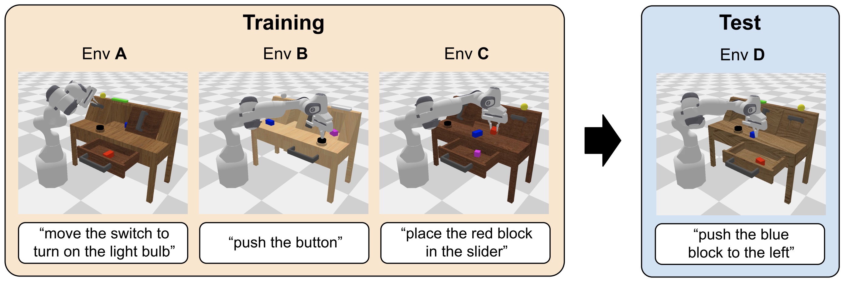
The importance of long-horizon evaluation becomes apparent when considering how individual skill failures accumulate. If each skill succeeds with probability $p$ and a task requires $K$ approximately independent successful skills, the probability of completing the entire task is:
\[P_{\mathrm{task}} \approx p^K\]
- For example, even with a per-skill success rate of $p=0.95$, completing $K=20$ consecutive skills yields an overall success probability of only $0.95^{20} \approx 0.36$.
Consequently, evaluation must extend beyond isolated skills to tasks requiring multiple sequential interactions. Short-horizon benchmarks alone can substantially overestimate a system’s readiness for autonomous deployment.

Sequence-Length Metrics

Sequence-Length Metrics is informative only when the evaluation distribution, success criteria, intervention policy, and trial protocol are explicit. Aggregate scores should be paired with failure categories and scenario coverage so improvements are not caused by easier task mixes or hidden changes in evaluation conditions.
Sequence-Length Metrics should expose how reliability changes as more decisions are composed, because per-step competence can translate into sharply lower end-to-end success over long trajectories.
For tasks containing multiple instructions, define maximum completed prefix:
\[L_i = \max \{ k: g_1,\ldots,g_k \text{ completed} \}\]
Average sequence length is
\[\bar L = \frac{1}{N} \sum_i L_i\]
CALVIN: A Benchmark for Language-Conditioned Policy Learning for Long-Horizon Robot Manipulation Tasks by Mees et al. (2022) evaluates language-conditioned policies on chains of sequential manipulation instructions, explicitly emphasizing long-horizon execution and zero-shot generalization to novel language and environments.
This exposes a capability that single-task success cannot measure:
\[\boxed{ \text{Can the agent keep succeeding?} }\]

Evaluating Generalization

Evaluating Generalization requires holding out the specific factor of interest, such as object, task, scene, language, or embodiment, so apparent transfer is not confounded by overlap elsewhere in the benchmark.
Evaluating Generalization should report the task distribution, trial protocol, failure criteria, and interaction budget explicitly so improvements can be attributed to capability rather than easier scenarios or hidden assistance.
A generalist Physical AI model should be evaluated outside its exact training distribution. The training stage should therefore be interpreted by the capability it is intended to add: broad representations, embodiment grounding, task adaptation, or closed-loop behavioral improvement.
Let training distribution be
\[p_{\mathrm{train}}( o,g,e )\]
- and test distribution be
  \[p_{\mathrm{test}}( o,g,e )\]
Evaluation should systematically vary:
\[\text{objects}, \quad \text{instructions}, \quad \text{environments}, \quad \text{embodiments}, \quad \text{dynamics}\]
A useful evaluation matrix is:
Dimension In-distribution Generalization ———– ——————— —————- Object Seen object Novel object Task Seen task Novel task Language Seen phrasing Novel phrasing Scene Seen scene Novel scene Robot Training embodiment New embodiment Dynamics Nominal Perturbed
The distinction between memorization and generalization is therefore explicit. The metric should consequently be read together with the task distribution, horizon, intervention policy, and whether the measurement was obtained in simulation or on physical hardware.

Object Generalization

Object Generalization tests whether a policy can apply learned manipulation concepts to unseen instances or categories without relying on memorized appearance or object-specific trajectories.
Object Generalization should report the task distribution, trial protocol, failure criteria, and interaction budget explicitly so improvements can be attributed to capability rather than easier scenarios or hidden assistance.
Suppose training contains:
\[\mathcal{O}_{\mathrm{train}} = \{ o_1,\ldots,o_n \}\]
Evaluation samples:
\[o^* \notin \mathcal{O}_{\mathrm{train}}\]
Measure:
\[\operatorname{SR}_{\mathrm{novel\ object}}\]
A stronger test changes not only visual appearance but physical properties:
\[\text{shape}, \quad \text{mass}, \quad \text{size}, \quad \text{compliance}, \quad \text{friction}\]
This separates semantic object recognition from actual physical generalization. For embodied use, that semantic interpretation must remain tied to the current scene, the robot state, and the actions that are actually feasible for the embodiment.

Generalization and Robustness

This section connects language generalization with environment generalization. The discussion develops the relevant methods, implementation details, and practical tradeoffs.

Language Generalization

Language Generalization measures whether new phrasings and compositional instructions map to the same physical intent, separating linguistic transfer from memorized command templates.
Language Generalization should report the task distribution, trial protocol, failure criteria, and interaction budget explicitly so improvements can be attributed to capability rather than easier scenarios or hidden assistance.
A language-conditioned robot should understand paraphrases. For embodied use, that semantic interpretation must remain tied to the current scene, the robot state, and the actions that are actually feasible for the embodiment.
For task goal $g$, define instruction set
\[L_g = \{ l_1,l_2,\ldots,l_M \}\]
For example:

Put the mug in the sink.
Move the cup into the sink.
Take the mug over to the sink.
Place this drinking cup inside the sink.

Evaluation should test whether
\[\pi(a\mid o,l_i)\]
- remains behaviorally consistent across valid linguistic realizations.
This matters because real users do not interact with robots using benchmark templates. For embodied use, that semantic interpretation must remain tied to the current scene, the robot state, and the actions that are actually feasible for the embodiment.

Environment Generalization

Environment Generalization asks whether behavior survives changes in layout, background, lighting, distractors, and object arrangement while preserving the task’s underlying physical structure.
Environment Generalization should report the task distribution, trial protocol, failure criteria, and interaction budget explicitly so improvements can be attributed to capability rather than easier scenarios or hidden assistance.
Train environments may contain:
\[E_{\mathrm{train}} = \{ e_1,\ldots,e_N \}\]
Test environment:
\[e^* \notin E_{\mathrm{train}}\]
Changes can include:
\[\text{layout}, \quad \text{lighting}, \quad \text{background}, \quad \text{clutter}, \quad \text{object placement}\]
The resulting metric
\[\operatorname{SR}_{\mathrm{novel\ env}}\]
- measures whether the policy learned transferable behavior rather than environment-specific correlations.

Compositional Generalization

Compositional Generalization evaluates whether skills and concepts learned separately can be recombined into new tasks, a stronger test than succeeding on new examples of familiar task templates.
Compositional Generalization should report the task distribution, trial protocol, failure criteria, and interaction budget explicitly so improvements can be attributed to capability rather than easier scenarios or hidden assistance.
An especially important test evaluates new combinations of known concepts. The metric should consequently be read together with the task distribution, horizon, intervention policy, and whether the measurement was obtained in simulation or on physical hardware.
Suppose training includes:
\[\text{pick(red cup)}\]
- and
  \[\text{place(blue bowl, sink)}\]
A compositional test might request:
\[\text{place(red cup, sink)}\]
The individual concepts are familiar, but the combination is new. The stronger test is whether the learned representation and policy continue to work when several factors shift together rather than when only one superficial attribute changes.
Formally:
\[g^* \notin G_{\mathrm{train}}\]
- while
  \[\operatorname{components}(g^*) \subseteq \operatorname{components}(G_{\mathrm{train}})\]
This evaluates whether the system can recombine learned physical capabilities. The metric should consequently be read together with the task distribution, horizon, intervention policy, and whether the measurement was obtained in simulation or on physical hardware.

Lifelong and Knowledge-Transfer Evaluation

Lifelong and Knowledge-Transfer Evaluation is informative only when the evaluation distribution, success criteria, intervention policy, and trial protocol are explicit. Aggregate scores should be paired with failure categories and scenario coverage so improvements are not caused by easier task mixes or hidden changes in evaluation conditions.
Lifelong and Knowledge-Transfer Evaluation should report the task distribution, trial protocol, failure criteria, and interaction budget explicitly so improvements can be attributed to capability rather than easier scenarios or hidden assistance.
Physical agents may encounter new tasks continually. The metric should consequently be read together with the task distribution, horizon, intervention policy, and whether the measurement was obtained in simulation or on physical hardware.
Let task sequence be:
\[T_1,T_2,\ldots,T_K\]
After learning task $T_k$, evaluate performance on all earlier tasks:
\[R_{k,j}, \qquad j\leq k\]
This enables measurement of:
\[\text{forward transfer}, \quad \text{backward transfer}, \quad \text{catastrophic forgetting}\]
LIBERO: Benchmarking Knowledge Transfer for Lifelong Robot Learning by Liu et al. (2023) provides four suites totaling 130 manipulation tasks and explicitly studies transfer of declarative and procedural knowledge, task ordering, policy architecture, and the effects of pretraining.
For continually updated Physical AI systems, such evaluation becomes important because improving new capabilities should not silently degrade old ones. The metric should consequently be read together with the task distribution, horizon, intervention policy, and whether the measurement was obtained in simulation or on physical hardware.

Robustness Evaluation

Robustness Evaluation is informative only when the evaluation distribution, success criteria, intervention policy, and trial protocol are explicit. Aggregate scores should be paired with failure categories and scenario coverage so improvements are not caused by easier task mixes or hidden changes in evaluation conditions.
Robustness Evaluation should include controlled perturbations to sensing, objects, dynamics, timing, and instructions so performance reflects tolerance to plausible deployment variation rather than only nominal conditions.
A policy should be evaluated under controlled perturbations. This is the point where learned predictions meet coordinate frames, control rates, actuator limits, and the closed-loop dynamics of the physical system.
Let nominal environment parameters be
\[\phi_0\]
Perturbed evaluation uses
\[\phi = \phi_0+\delta\]
Possible perturbations include:
\[\text{camera movement}\] \[\text{lighting changes}\] \[\text{object displacement}\] \[\text{sensor noise}\] \[\text{latency}\] \[\text{actuator error}\]
Define robustness curve:
\[R(\delta) = \operatorname{SR}( \pi;\delta )\]
A robust policy should degrade gradually rather than collapse under small perturbations. This is the point where learned predictions meet coordinate frames, control rates, actuator limits, and the closed-loop dynamics of the physical system.

Perturbation Sweeps

Perturbation Sweeps changes the operating assumptions of the physical agent, so its value should be judged by the specific state information it exposes, the action or prediction it produces, and whether those outputs remain useful once the environment responds.
Perturbation Sweeps should define the task distribution, success criteria, intervention policy, and resource budget before comparison so measured gains are not artifacts of easier scenarios or hidden assistance.
Instead of evaluating at one perturbation magnitude, sweep:
\[\delta \in \{ \delta_1,\ldots,\delta_K \}\]
Then plot:
\[\operatorname{SR}(\delta)\]
A summary metric can integrate the curve:
\[\operatorname{AUC}_{\mathrm{robust}} = \int \operatorname{SR}(\delta) \,d\delta\]
This distinguishes two policies that have identical nominal success but very different failure sensitivity.

Recovery Evaluation

Recovery Evaluation becomes important because deployment changes the state distribution seen by the policy. Errors that are individually small can move the system into unfamiliar states, so robust control requires either broader data coverage, corrective examples, explicit recovery behavior, or online mechanisms that can re-establish a familiar state.
Recovery Evaluation should report the task distribution, trial protocol, failure criteria, and interaction budget explicitly so improvements can be attributed to capability rather than easier scenarios or hidden assistance.
A robust autonomous agent should recover from errors. The metric should consequently be read together with the task distribution, horizon, intervention policy, and whether the measurement was obtained in simulation or on physical hardware.
Evaluation can deliberately introduce disturbance at time $t$:
\[s_t \rightarrow s_t'\]
Examples include:
\[\text{move the target object}\] \[\text{cause a grasp to slip}\] \[\text{close an open drawer}\] \[\text{place an obstacle in the path}\]
Recovery rate is:
\[R_{\mathrm{recover}} = P( \text{eventual success} \mid \text{disturbance} )\]
This measures a fundamentally different capability from nominal task execution. The metric should consequently be read together with the task distribution, horizon, intervention policy, and whether the measurement was obtained in simulation or on physical hardware.

Time-to-Recovery

Time-to-Recovery becomes important because deployment changes the state distribution seen by the policy. Errors that are individually small can move the system into unfamiliar states, so robust control requires either broader data coverage, corrective examples, explicit recovery behavior, or online mechanisms that can re-establish a familiar state.
Time-to-recovery measures how quickly the agent returns to a viable trajectory after a disturbance or mistake, separating graceful degradation from failures that merely avoid termination.
Successful recovery can still be inefficient.
Let disturbance occur at
\[t_f\]
- and normal task progress resume at
  \[t_r\]
Recovery time is
\[T_{\mathrm{recover}} = t_r-t_f\]
Similarly, count additional actions:
\[A_{\mathrm{recover}} = N_{\mathrm{postfailure}} - N_{\mathrm{nominal}}\]
A capable autonomous system should both recover reliably and avoid repeatedly entering ineffective loops. A deployable system should separate learned behavioral competence from independently enforced limits so that policy uncertainty or distribution shift does not directly become unsafe actuation.

Recovery, Safety, and Efficiency

This section connects intervention rate with autonomy duration. The discussion develops the relevant methods, implementation details, and practical tradeoffs.

Intervention Rate

Intervention Rate changes the operating assumptions of the physical agent, so its value should be judged by the specific state information it exposes, the action or prediction it produces, and whether those outputs remain useful once the environment responds.
Intervention rate captures how often nominal autonomy still depends on a human or safety controller, complementing task success with a measure of operational independence.
For deployed systems, human intervention is a critical metric. The central distinction is the source of feedback and whether the learner can safely collect new trajectories, since that determines both the optimization objective and the distribution of states available for improvement.
Let
\[I_i = \text{number of interventions during episode }i\]
Intervention rate can be measured as:
\[R_I = \frac{\sum_i I_i} {\sum_i T_i}\]
Depending on the domain, the denominator might be:
\[\text{hours}, \quad \text{kilometers}, \quad \text{tasks}, \quad \text{actions}\]
A useful autonomy system should reduce intervention frequency while maintaining safety and task success. A deployable system should separate learned behavioral competence from independently enforced limits so that policy uncertainty or distribution shift does not directly become unsafe actuation.

Autonomy Duration

Autonomy Duration changes the operating assumptions of the physical agent, so its value should be judged by the specific state information it exposes, the action or prediction it produces, and whether those outputs remain useful once the environment responds.
Autonomy Duration benefits from explicit progress and completion signals so the agent can tell whether a subgoal actually changed the world as intended, rather than assuming that a plausible sequence of actions will compose successfully.
Another deployment metric is uninterrupted autonomous operation. The metric should consequently be read together with the task distribution, horizon, intervention policy, and whether the measurement was obtained in simulation or on physical hardware.
Let
\[T_i = \text{time until intervention or unrecoverable failure}\]
Then:
\[\operatorname{MTBI} = \frac{1}{N} \sum_i T_i\]
- where MTBI denotes mean time between interventions.
For long-running robots, this may be more informative than isolated episode success. Reliable autonomy therefore requires explicit progress state, completion conditions, and recovery behavior rather than assuming that a plausible next action will compose into a successful long-horizon trajectory.
A robot that completes 95% of short benchmark tasks may still be impractical if it requires human assistance every few minutes. The metric should consequently be read together with the task distribution, horizon, intervention policy, and whether the measurement was obtained in simulation or on physical hardware.

Safety Metrics

Safety Metrics is informative only when the evaluation distribution, success criteria, intervention policy, and trial protocol are explicit. Aggregate scores should be paired with failure categories and scenario coverage so improvements are not caused by easier task mixes or hidden changes in evaluation conditions.
Safety Metrics requires enforcement outside the learned policy for constraints that must hold even when the model is uncertain, out of distribution, or wrong.
Task success must be evaluated jointly with safety. A deployable system should separate learned behavioral competence from independently enforced limits so that policy uncertainty or distribution shift does not directly become unsafe actuation.
Define violation indicators:
\[C_{\mathrm{collision}}, \quad C_{\mathrm{force}}, \quad C_{\mathrm{workspace}}, \quad C_{\mathrm{human}}, \quad C_{\mathrm{rule}}\]
Safety violation rate can be:
\[V = \frac{ \sum_i \mathbb{1}[ \text{safety violation in episode }i ] }{ N }\]
Task reward should not allow unsafe behavior to be hidden by high success. The central distinction is the source of feedback and whether the learner can safely collect new trajectories, since that determines both the optimization objective and the distribution of states available for improvement.
A useful evaluation reports:
\[\boxed{ \text{Success} \quad\text{and}\quad \text{Safety} }\]
- separately.

Severity-Weighted Safety

Severity-Weighted Safety should be implemented as a system property rather than inferred from average policy success. Learned behavior, uncertainty estimates, runtime constraints, independent monitors, and fallback behavior provide complementary layers because they fail under different assumptions.
Severity-Weighted Safety requires enforcement outside the learned policy for constraints that must hold even when the model is uncertain, out of distribution, or wrong.
Not all failures have equal consequence.
Assign severity:
\[w_j\]
- to event type $j$.
Then:
\[R_{\mathrm{risk}} = \sum_j w_j P(E_j)\]
For example, gently contacting a table should not necessarily receive the same weight as contacting a person.
This is particularly important in autonomous driving and human-robot interaction, where low-frequency high-severity events dominate deployment risk. This is the point where learned predictions meet coordinate frames, control rates, actuator limits, and the closed-loop dynamics of the physical system.

Constraint-Based Evaluation

Constraint-Based Evaluation is informative only when the evaluation distribution, success criteria, intervention policy, and trial protocol are explicit. Aggregate scores should be paired with failure categories and scenario coverage so improvements are not caused by easier task mixes or hidden changes in evaluation conditions.
Constraint-Based Evaluation requires enforcement outside the learned policy for constraints that must hold even when the model is uncertain, out of distribution, or wrong.
Safety can also be expressed as constraints:
\[C_j(\tau) \leq c_j\]
For example:
\[F_{\mathrm{contact}} < F_{\max}\] \[d_{\mathrm{human}} > d_{\min}\] \[v < v_{\max}\]
A trajectory can therefore be classified as successful only if
\[R_{\mathrm{task}}(\tau) \geq r_{\min}\]
- and
  \[C_j(\tau) \leq c_j \quad \forall j\]
This prevents reward tradeoffs from treating certain safety constraints as optional. The training stage should therefore be interpreted by the capability it is intended to add: broad representations, embodiment grounding, task adaptation, or closed-loop behavioral improvement.

Efficiency Metrics

Efficiency Metrics is informative only when the evaluation distribution, success criteria, intervention policy, and trial protocol are explicit. Aggregate scores should be paired with failure categories and scenario coverage so improvements are not caused by easier task mixes or hidden changes in evaluation conditions.
Efficiency Metrics should report the task distribution, trial protocol, failure criteria, and interaction budget explicitly so improvements can be attributed to capability rather than easier scenarios or hidden assistance.
A robot can complete a task successfully but inefficiently. The metric should consequently be read together with the task distribution, horizon, intervention policy, and whether the measurement was obtained in simulation or on physical hardware.
Useful efficiency measures include:
\[T_{\mathrm{completion}}\] \[N_{\mathrm{actions}}\] \[L_{\mathrm{path}}\] \[E_{\mathrm{energy}}\]
Normalized path efficiency can be:
\[\eta_{\mathrm{path}} = \frac{ L_{\mathrm{optimal}} }{ L_{\mathrm{executed}} }\]
Similarly, action efficiency can compare actual action count with a reference:
\[\eta_{\mathrm{action}} = \frac{ N_{\mathrm{reference}} }{ N_{\mathrm{executed}} }\]
Efficiency matters because unnecessarily long physical trajectories consume time, energy, actuator lifetime, and potentially user patience. This is the point where learned predictions meet coordinate frames, control rates, actuator limits, and the closed-loop dynamics of the physical system.

Success Weighted by Efficiency

Success Weighted by Efficiency is informative only when the evaluation distribution, success criteria, intervention policy, and trial protocol are explicit. Aggregate scores should be paired with failure categories and scenario coverage so improvements are not caused by easier task mixes or hidden changes in evaluation conditions.
Success weighted by efficiency distinguishes policies that complete the task economically from those that succeed only through excessive motion, retries, model calls, or human assistance.
Navigation benchmarks often motivate metrics that combine success and efficiency. The metric should consequently be read together with the task distribution, horizon, intervention policy, and whether the measurement was obtained in simulation or on physical hardware.
A general form is:
\[M = S \cdot \frac{ C^* }{ \max(C,C^*) }\]
- where:
$S$ indicates success. $C$ is actual execution cost. $C^*$ is reference cost. The same principle can be applied to manipulation using trajectory length, execution time, or energy.
This distinguishes:
\[\text{successful and efficient}\]
- from
  \[\text{successful but wasteful}\]

Evaluation of Vision-Language-Action Models

VLA evaluation should separate semantic understanding from physical execution by measuring task success, robustness to scene and instruction shifts, action validity, recovery behavior, and closed-loop performance rather than relying on offline action-prediction error alone.
Evaluation of Vision-Language-Action Models should report the task distribution, trial protocol, failure criteria, and interaction budget explicitly so improvements can be attributed to capability rather than easier scenarios or hidden assistance.
A VLA should be evaluated across several dimensions:
\[\boxed{ \begin{array}{c} \text{Language Understanding}\\ \text{Visual Grounding}\\ \text{Manipulation Skill}\\ \text{Action Precision}\\ \text{Generalization}\\ \text{Long-Horizon Execution}\\ \text{Recovery} \end{array} }\]
A single aggregate task-success number cannot determine which component limits performance. In practice, the representation must preserve the task-relevant geometry, state, and uncertainty needed by downstream reasoning and control rather than only semantic appearance.
Evaluation suites should therefore isolate capability dimensions where possible. In practice, the representation must preserve the task-relevant geometry, state, and uncertainty needed by downstream reasoning and control rather than only semantic appearance.

LIBERO

LIBERO is informative only when the evaluation distribution, success criteria, intervention policy, and trial protocol are explicit. Aggregate scores should be paired with failure categories and scenario coverage so improvements are not caused by easier task mixes or hidden changes in evaluation conditions.
LIBERO should define the task distribution, success criteria, intervention policy, and resource budget before comparison so measured gains are not artifacts of easier scenarios or hidden assistance.
LIBERO focuses on lifelong robot manipulation and knowledge transfer. Its benchmark contains four suites with 130 tasks and human-teleoperated demonstrations, with experiments designed around transfer, pretraining, task ordering, and continual learning. Its suites allow evaluation of different forms of generalization and transfer rather than treating robot manipulation as a single homogeneous task distribution.
For modern VLAs, LIBERO has consequently become useful for testing whether pretrained representations and policies can adapt to downstream manipulation tasks. The training stage should therefore be interpreted by the capability it is intended to add: broad representations, embodiment grounding, task adaptation, or closed-loop behavioral improvement.

Robot Foundation-Model Benchmarks

This section connects calvin with behavior-1k. The discussion develops the relevant methods, implementation details, and practical tradeoffs.

CALVIN

CALVIN is informative only when the evaluation distribution, success criteria, intervention policy, and trial protocol are explicit. Aggregate scores should be paired with failure categories and scenario coverage so improvements are not caused by easier task mixes or hidden changes in evaluation conditions.
CALVIN should define the task distribution, success criteria, intervention policy, and resource budget before comparison so measured gains are not artifacts of easier scenarios or hidden assistance.
CALVIN focuses on language-conditioned long-horizon manipulation. For embodied use, that semantic interpretation must remain tied to the current scene, the robot state, and the actions that are actually feasible for the embodiment.
A typical evaluation asks the agent to complete a chain:
\[[ g_1, g_2, g_3, g_4, g_5 ]\]
Metrics include success after one through five sequential instructions and average completed sequence length. The benchmark also evaluates generalization to novel language, environments, and objects.
CALVIN therefore stresses temporal composition:
\[\boxed{ \text{Can individually learned skills be chained reliably?} }\]

BEHAVIOR-1K

BEHAVIOR-1K is informative only when the evaluation distribution, success criteria, intervention policy, and trial protocol are explicit. Aggregate scores should be paired with failure categories and scenario coverage so improvements are not caused by easier task mixes or hidden changes in evaluation conditions.
BEHAVIOR-1K should define the task distribution, success criteria, intervention policy, and resource budget before comparison so measured gains are not artifacts of easier scenarios or hidden assistance.
BEHAVIOR-1K expands evaluation toward household-scale embodied intelligence. The benchmark contains 1,000 everyday activities instantiated in 50 interactive scenes with more than 10,000 objects, with tasks grounded in surveys of activities people actually perform and want assistance with.
The scale changes the evaluation target from narrow manipulation toward:
\[\text{navigation} + \text{manipulation} + \text{state tracking} + \text{long-horizon planning}\]
Examples such as cooking, cleaning, and organizing naturally require many interacting skills and environmental state changes. A useful plan therefore has to connect high-level intent to reachable intermediate states and leave room to replan when execution produces an unexpected observation.

Simulation Versus Real-World Evaluation

Simulation Versus Real-World Evaluation models how physical state evolves under actions, enabling counterfactual prediction, planning, synthetic experience, and closed-loop evaluation before every decision is attempted in the real world.
Simulation Versus Real-World Evaluation should vary or calibrate the physical and sensing factors that materially affect the deployed policy, with success measured by transfer to held-out real behavior rather than by simulator performance alone.
Simulation provides reproducibility:
\[E_i = \operatorname{Reset}( \text{seed}_i )\]
Policies can therefore be compared under identical conditions. The practical question is whether the generated variation covers the geometry, dynamics, sensing, and timing errors that materially affect transfer to the real system.
Real-world evaluation samples from:
\[p_{\mathrm{real}}(s,o,d)\]
- where $d$ includes uncontrolled disturbances.
Simulation is useful for:
\[\text{scale}, \quad \text{repeatability}, \quad \text{rare events}, \quad \text{controlled perturbations}\]
Real-world evaluation is required to reveal:
\[\text{reality-gap failures}, \quad \text{hardware failures}, \quad \text{unmodeled dynamics}, \quad \text{real perception errors}\]
Neither should replace the other.
RoboLab: A High-Fidelity Simulation Benchmark for Analysis of Task Generalist Policies by Yang et al. (2026) provides a complementary simulation benchmark for task-generalist robot policies. RoboLab-120 contains 120 tabletop manipulation tasks evaluated in Isaac Lab, including multiple language formulations for each task, and is designed to support repeatable policy comparison without requiring every evaluation to be run on physical hardware.
FLUX 3 Action reported 515 successful trials out of 1,200 on RoboLab-120, corresponding to 42.9% success and first place on the public leaderboard at release. The result should be interpreted as simulation-benchmark performance rather than direct evidence of equivalent real-world robustness, because simulation fidelity, task composition, and policy-specific distribution shift can alter rankings.
Real-robot evidence should therefore be reported separately. FLUX 3 Action additionally reports blind third-party Franka evaluation on ten single-object DROID tasks, completing 28 of 30 attempts. Simulation success and physical success answer different questions and should not be collapsed into one metric:
\[\boxed{ \text{Simulation Benchmark} \neq \text{Real-Robot Validation} }\]
Runtime comparisons also require separating per-call latency from the amount of motion produced by each call. FLUX 3 Action predicts 32 actions at 15 Hz, corresponding to approximately 2.13 seconds of planned motion, so a useful deployment metric is the real-time factor:
\[\mathrm{RTF} = \frac{T_{\mathrm{inference}}}{T_{\mathrm{action\ chunk}}}\]
Reporting task success, real-time factor, inference latency, action-horizon duration, memory requirements, and physical-robot success separately makes comparisons between WAMs and VLAs substantially more informative. This is the point where learned predictions meet coordinate frames, control rates, actuator limits, and the closed-loop dynamics of the physical system.

SimplerEnv and Real-to-Sim Evaluation

SimplerEnv and Real-to-Sim Evaluation is informative only when the evaluation distribution, success criteria, intervention policy, and trial protocol are explicit. Aggregate scores should be paired with failure categories and scenario coverage so improvements are not caused by easier task mixes or hidden changes in evaluation conditions.
SimplerEnv and Real-to-Sim Evaluation should vary or calibrate the physical and sensing factors that materially affect the deployed policy, with success measured by transfer to held-out real behavior rather than by simulator performance alone.
SIMPLER evaluates real-world manipulation policies such as RT-1, RT-1-X, and Octo in simulated replicas of real robot setups. It provides both visual-matching evaluation and variant-aggregation evaluation, where multiple backgrounds, lighting conditions, distractors, and textures are aggregated.
The following figure (source) shows SIMPLER’s simulation-based evaluation procedure and comparison of simulated and real-world robot-policy performance. Characterizing generalist robot manipulation policies typically involves evaluating them on many tasks across many scenarios, a laborious undertaking in the real world (top left). SIMPLER offers an evaluation procedure in which policies trained on real data are evaluated in purpose-built simulated environments (bottom left). Our approach yields a strong correlation between real-world and simulated performance (right) for various open-source robot policies across two commonly used robot embodiments (Google Robot and WidowX) and over ∼1500 evaluation episodes. These results highlight the potential of simulation-based approaches for evaluating generalist real-world robot manipulation policies in a scalable, reproducible, and reliable way.

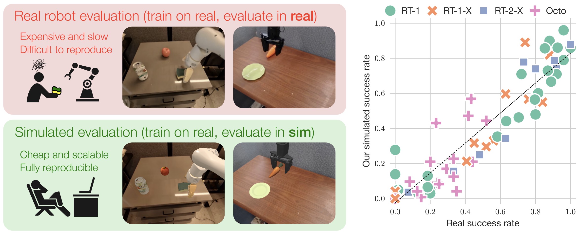
This introduces an important evaluation question:
\[\operatorname{Corr} ( R_{\mathrm{sim}}, R_{\mathrm{real}} )\]
A simulator is useful as a policy benchmark only if relative performance in simulation provides meaningful information about real-world performance. This is the point where learned predictions meet coordinate frames, control rates, actuator limits, and the closed-loop dynamics of the physical system.
Thus simulation evaluation itself must be validated. The practical question is whether the generated variation covers the geometry, dynamics, sensing, and timing errors that materially affect transfer to the real system.

Evaluating Sim-to-Real Correlation

Evaluating Sim-to-Real Correlation changes the operating assumptions of the physical agent, so its value should be judged by the specific state information it exposes, the action or prediction it produces, and whether those outputs remain useful once the environment responds.
Evaluating Sim-to-Real Correlation should vary or calibrate the physical and sensing factors that materially affect the deployed policy, with success measured by transfer to held-out real behavior rather than by simulator performance alone.
Suppose policies
\[\Pi = \{ \pi_1,\ldots,\pi_K \}\]
- have simulated scores
  \[S_i\]
  - and real scores
    \[R_i\]
Measure ranking correlation:
\[\rho = \operatorname{Spearman} ( S,R )\]
High
\[\rho\]
- means the simulator preserves policy ranking even if absolute success rates differ.
This may be more useful than requiring:
\[S_i \approx R_i\]
For model development, knowing that an improvement in simulation is likely to remain an improvement in reality can make large-scale simulated evaluation useful. The practical question is whether the generated variation covers the geometry, dynamics, sensing, and timing errors that materially affect transfer to the real system.

Autonomous Driving Evaluation

Autonomous Driving Evaluation must account for the fact that an autonomous vehicle changes the future scene through its own motion and through the reactions of other agents. Closed-loop evaluation is therefore essential for separating trajectories that look plausible in recorded logs from policies that remain safe and effective under interaction.
Autonomous Driving Evaluation should report the task distribution, trial protocol, failure criteria, and interaction budget explicitly so improvements can be attributed to capability rather than easier scenarios or hidden assistance.
Autonomous driving illustrates especially clearly why open-loop trajectory metrics are insufficient. This is the point where learned predictions meet coordinate frames, control rates, actuator limits, and the closed-loop dynamics of the physical system.
A planner may predict trajectory
\[\hat\tau\]
- that differs from recorded human trajectory
  \[\tau^*\]
A displacement metric such as
\[\operatorname{ADE} = \frac{1}{T} \sum_t \| \hat x_t-x_t^* \|_2\]
- measures imitation accuracy, not necessarily driving quality.
A different trajectory may be completely safe. This is the point where learned predictions meet coordinate frames, control rates, actuator limits, and the closed-loop dynamics of the physical system.
Conversely, a trajectory close to the recorded human path may lead to collision once other agents react to it. This is the point where learned predictions meet coordinate frames, control rates, actuator limits, and the closed-loop dynamics of the physical system.

nuPlan

nuPlan changes the operating assumptions of the physical agent, so its value should be judged by the specific state information it exposes, the action or prediction it produces, and whether those outputs remain useful once the environment responds.
nuPlan should define the task distribution, success criteria, intervention policy, and resource budget before comparison so measured gains are not artifacts of easier scenarios or hidden assistance.
nuPlan: A Closed-Loop ML-Based Planning Benchmark for Autonomous Vehicles by Caesar et al. (2021) was introduced specifically to address limitations of open-loop planning evaluation. It combines a large-scale driving dataset, a lightweight closed-loop simulator, reactive agents, and planning-specific metrics.
The central evaluation loop is:
\[\text{Planner} \rightarrow \text{Ego Action} \rightarrow \text{Simulation} \rightarrow \text{Updated Traffic} \rightarrow \text{Planner}\]
This evaluates the consequences of the planner’s own decisions rather than merely comparing predictions against logged human trajectories. A useful plan therefore has to connect high-level intent to reachable intermediate states and leave room to replan when execution produces an unexpected observation.

Interactive Driving Evaluation

Interactive Driving Evaluation must account for the fact that an autonomous vehicle changes the future scene through its own motion and through the reactions of other agents. Closed-loop evaluation is therefore essential for separating trajectories that look plausible in recorded logs from policies that remain safe and effective under interaction.
Interactive Driving Evaluation should report the task distribution, trial protocol, failure criteria, and interaction budget explicitly so improvements can be attributed to capability rather than easier scenarios or hidden assistance.
Closed-loop driving evaluation must model other agents reacting to the ego vehicle. Because each executed command changes the next input distribution, the relevant unit of evaluation is the resulting rollout rather than an isolated one-step prediction.
Let ego action be:
\[a_t^{\mathrm{ego}}\]
Other agents respond:
\[a_t^{j} \sim \pi_j( s_t,a_t^{\mathrm{ego}} )\]
The transition is therefore:
\[s_{t+1} = F( s_t, a_t^{\mathrm{ego}}, a_t^1,\ldots,a_t^N )\]
A static replay of recorded traffic cannot fully represent this interaction because logged agents do not react to counterfactual ego behavior. This is the point where learned predictions meet coordinate frames, control rates, actuator limits, and the closed-loop dynamics of the physical system.
Recent work such as nuPlan-R by Peng et al. (2025) extends closed-loop evaluation with learned reactive multi-agent simulation, motivated by limitations of rule-based reactive traffic agents in representing diverse interactions.

Waymo Open Dataset Evaluation

Waymo Open Dataset Evaluation is informative only when the evaluation distribution, success criteria, intervention policy, and trial protocol are explicit. Aggregate scores should be paired with failure categories and scenario coverage so improvements are not caused by easier task mixes or hidden changes in evaluation conditions.
Waymo Open Dataset Evaluation should be assessed by the new behavioral coverage it contributes, especially rare states, recovery situations, and observation-action combinations that are missing from the current training distribution.
The Waymo Open Dataset Challenges span perception, motion prediction, interaction prediction, occupancy and flow, scenario generation, simulated agents, and vision-based end-to-end driving. Its leaderboards remain active even though Waymo is not hosting formal challenges in 2026.
The breadth illustrates how autonomous-driving evaluation has expanded from isolated perception toward:
\[\boxed{ \text{Perception} \rightarrow \text{Prediction} \rightarrow \text{Simulation} \rightarrow \text{End-to-End Driving}. }\]
Physical AI evaluation increasingly follows the same trajectory. This is the point where learned predictions meet coordinate frames, control rates, actuator limits, and the closed-loop dynamics of the physical system.

Sim-to-Real and Driving Evaluation

This section connects evaluating world models with evaluating world models by decision quality. The discussion develops the relevant methods, implementation details, and practical tradeoffs.

Evaluating World Models

Evaluating World Models should be judged by whether predicted futures rank or reject candidate actions correctly, not only by pixel similarity, because small visual errors may be harmless while small contact errors can reverse a control decision.
Evaluating World Models should optimize for decision-relevant prediction: contact, geometry, timing, and task progress matter when they change which action is preferred, whereas visually conspicuous errors may be harmless if they do not affect control.
A world model predicts:
\[\hat s_{t+1} = M_\phi( s_t,a_t )\]
One-step prediction error is:
\[E_1 = d( \hat s_{t+1}, s_{t+1} )\]
But physical usefulness depends on longer rollouts:
\[\hat s_{t+H} = M_\phi^{(H)} ( s_t,a_{t:t+H-1} )\]
Evaluate:
\[E_H = d( \hat s_{t+H}, s_{t+H} )\]
Because errors compound, evaluation should sweep horizon:
\[H \in \{ 1,5,10,50,\ldots \}\]
A world model useful for planning must preserve action-conditioned consequences over the horizon relevant to decisions. A useful plan therefore has to connect high-level intent to reachable intermediate states and leave room to replan when execution produces an unexpected observation.

Evaluating World Models by Decision Quality

Evaluating World Models by Decision Quality should be judged by whether predicted futures rank or reject candidate actions correctly, not only by pixel similarity, because small visual errors may be harmless while small contact errors can reverse a control decision.
Evaluating World Models by Decision Quality should optimize for decision-relevant prediction: contact, geometry, timing, and task progress matter when they change which action is preferred, whereas visually conspicuous errors may be harmless if they do not affect control.
Pixel reconstruction quality alone may not indicate whether a world model is useful. Its usefulness therefore depends less on visual plausibility alone than on whether predicted state changes preserve the consequences that would alter a downstream decision.
Suppose two world models produce:
\[M_1, \quad M_2\]
Even if:
\[E_{\mathrm{pixel}}(M_1) < E_{\mathrm{pixel}}(M_2)\]
- the second may preserve task-relevant geometry and dynamics better.
A stronger evaluation measures downstream planning:
\[R_{\mathrm{plan}}( M_\phi )\]
Thus:
\[\boxed{ \text{World-model quality} = \text{predictive accuracy} + \text{decision usefulness}. }\]

Counterfactual Evaluation

Counterfactual Evaluation is informative only when the evaluation distribution, success criteria, intervention policy, and trial protocol are explicit. Aggregate scores should be paired with failure categories and scenario coverage so improvements are not caused by easier task mixes or hidden changes in evaluation conditions.
Counterfactual Evaluation should be judged by whether the model preserves the relative consequences of alternative actions, even if their rendered futures are not pixel-perfect.
A particularly difficult capability is counterfactual accuracy. The metric should consequently be read together with the task distribution, horizon, intervention policy, and whether the measurement was obtained in simulation or on physical hardware.
Given identical history:
\[h_t\]
- consider alternative actions:
  \[a_t^{(1)}, a_t^{(2)}\]
A world model should predict distinct consequences:
\[\hat s_{t+1}^{(1)} = M( h_t,a_t^{(1)} )\] \[\hat s_{t+1}^{(2)} = M( h_t,a_t^{(2)} )\]
Evaluation should determine whether these action-dependent differences correspond to real physical outcomes. This is the point where learned predictions meet coordinate frames, control rates, actuator limits, and the closed-loop dynamics of the physical system.
Without this capability, visually plausible generation may still be useless for planning. In practice, the representation must preserve the task-relevant geometry, state, and uncertainty needed by downstream reasoning and control rather than only semantic appearance.

Evaluating Agentic Physical AI

Evaluating Agentic Physical AI extends Physical AI beyond one-step control by adding persistent state, decomposition, tool or agent selection, and feedback-driven revision around the underlying motor policies.
Evaluating Agentic Physical AI should report the task distribution, trial protocol, failure criteria, and interaction budget explicitly so improvements can be attributed to capability rather than easier scenarios or hidden assistance.
Agentic systems introduce another layer of metrics. The metric should consequently be read together with the task distribution, horizon, intervention policy, and whether the measurement was obtained in simulation or on physical hardware.
A complete agent may perform:
\[\text{Reason} \rightarrow \text{Plan} \rightarrow \text{Tool Call} \rightarrow \text{Skill} \rightarrow \text{Verify} \rightarrow \text{Replan}\]
Evaluation should separately measure:
\[\text{planning accuracy}\] \[\text{skill-selection accuracy}\] \[\text{tool-use success}\] \[\text{failure detection}\] \[\text{recovery success}\] \[\text{final task completion}\]
This allows failure attribution rather than treating every unsuccessful episode as a policy failure. This is the point where learned predictions meet coordinate frames, control rates, actuator limits, and the closed-loop dynamics of the physical system.

Failure Taxonomy

Failure Taxonomy changes the operating assumptions of the physical agent, so its value should be judged by the specific state information it exposes, the action or prediction it produces, and whether those outputs remain useful once the environment responds.
Failure Taxonomy should define the task distribution, success criteria, intervention policy, and resource budget before comparison so measured gains are not artifacts of easier scenarios or hidden assistance.
For each unsuccessful episode, assign failure category:
\[F \in \{ F_{\mathrm{perception}}, F_{\mathrm{reasoning}}, F_{\mathrm{planning}}, F_{\mathrm{control}}, F_{\mathrm{tool}}, F_{\mathrm{recovery}}, F_{\mathrm{safety}} \}\]
Estimate:
\[P(F_j)\]
This produces a failure distribution:
\[\mathbf{f} = [ p_1,\ldots,p_K ]\]
A model update should ideally reduce specific components rather than merely move the aggregate success number.
Failure taxonomy therefore connects evaluation directly to post-training. The training stage should therefore be interpreted by the capability it is intended to add: broad representations, embodiment grounding, task adaptation, or closed-loop behavioral improvement.

Conditional Metrics

Conditional Metrics is informative only when the evaluation distribution, success criteria, intervention policy, and trial protocol are explicit. Aggregate scores should be paired with failure categories and scenario coverage so improvements are not caused by easier task mixes or hidden changes in evaluation conditions.
Conditional Metrics should report the task distribution, trial protocol, failure criteria, and interaction budget explicitly so improvements can be attributed to capability rather than easier scenarios or hidden assistance.
Aggregate success can hide important subpopulation failures. The metric should consequently be read together with the task distribution, horizon, intervention policy, and whether the measurement was obtained in simulation or on physical hardware.
Let metadata variable be:
\[z \in \{ \text{object type}, \text{task}, \text{scene}, \text{lighting}, \text{robot}, \text{difficulty} \}\]
Measure:
\[\operatorname{SR}(z)\]
For example:
\[\operatorname{SR}_{\mathrm{transparent\ objects}}\]
- may be much lower than overall success.
Conditional evaluation identifies capability gaps that would otherwise disappear inside averages. The metric should consequently be read together with the task distribution, horizon, intervention policy, and whether the measurement was obtained in simulation or on physical hardware.

Confidence Intervals

Confidence Intervals changes the operating assumptions of the physical agent, so its value should be judged by the specific state information it exposes, the action or prediction it produces, and whether those outputs remain useful once the environment responds.
Confidence intervals are essential when physical trials are limited or stochastic, because a small observed gain may reflect run-to-run variance rather than a reproducible improvement.
Physical evaluations are often expensive, producing relatively small sample sizes. The metric should consequently be read together with the task distribution, horizon, intervention policy, and whether the measurement was obtained in simulation or on physical hardware.
If success rate is:
\[\hat p = \frac{k}{N}\]
- the estimate has uncertainty.
Evaluation should report:
\[\hat p \pm \mathrm{CI}\]
When comparing policies $A$ and $B$, paired evaluation is particularly valuable:
\[\Delta_i = S_i^A-S_i^B\]
The comparison should estimate uncertainty over:
\[\bar\Delta\]
Without uncertainty estimates, small apparent improvements may simply reflect evaluation noise. The metric should consequently be read together with the task distribution, horizon, intervention policy, and whether the measurement was obtained in simulation or on physical hardware.

Repeated Trials

Repeated Trials changes the operating assumptions of the physical agent, so its value should be judged by the specific state information it exposes, the action or prediction it produces, and whether those outputs remain useful once the environment responds.
Repeated trials reveal variance caused by stochastic policies, perception noise, contact dynamics, and initialization, preventing a single lucky execution from being mistaken for robust capability.
Physical environments are stochastic.
For scenario $e_i$, run:
\[K\]
- trials:
  \[S_{i,1},\ldots,S_{i,K}\]
Estimate:
\[\hat p_i = \frac{1}{K} \sum_k S_{i,k}\]
Repeated trials are especially important when:
\[\text{object initialization}, \quad \text{grasp contact}, \quad \text{sensor noise}, \quad \text{policy sampling}\]
- introduce variability.
A single successful demonstration is not sufficient evidence of robust capability. What matters is not only the number of examples but also their coverage of tasks, embodiments, recovery states, and observation-action alignments that the deployed policy will encounter.

Agentic and Statistical Evaluation

This section connects deterministic versus stochastic policy evaluation with tail-risk evaluation. The discussion develops the relevant methods, implementation details, and practical tradeoffs.

Deterministic Versus Stochastic Policy Evaluation

Deterministic Versus Stochastic Policy Evaluation is informative only when the evaluation distribution, success criteria, intervention policy, and trial protocol are explicit. Aggregate scores should be paired with failure categories and scenario coverage so improvements are not caused by easier task mixes or hidden changes in evaluation conditions.
Deterministic Versus Stochastic Policy Evaluation should report the task distribution, trial protocol, failure criteria, and interaction budget explicitly so improvements can be attributed to capability rather than easier scenarios or hidden assistance.
Generative policies may sample actions:
\[a_t \sim \pi_\theta( a_t\mid o_t )\]
A deterministic evaluation with one random seed measures only one realization. This is the point where learned predictions meet coordinate frames, control rates, actuator limits, and the closed-loop dynamics of the physical system.
Instead evaluate:
\[\{ \tau_1,\ldots,\tau_K \} \sim \pi_\theta\]
Then estimate:
\[\mathbb{E}[R]\]
- and potentially:
  \[\operatorname{Var}(R)\]
For safety-critical settings, tail behavior may matter more than average performance. This is the point where learned predictions meet coordinate frames, control rates, actuator limits, and the closed-loop dynamics of the physical system.

Tail-Risk Evaluation

Tail-Risk Evaluation is informative only when the evaluation distribution, success criteria, intervention policy, and trial protocol are explicit. Aggregate scores should be paired with failure categories and scenario coverage so improvements are not caused by easier task mixes or hidden changes in evaluation conditions.
Tail-Risk Evaluation requires enforcement outside the learned policy for constraints that must hold even when the model is uncertain, out of distribution, or wrong.
Suppose return distribution is:
\[R \sim p(R)\]
Average:
\[\mathbb{E}[R]\]
- may hide rare catastrophic outcomes.
A tail-risk metric can examine:
\[\operatorname{CVaR}_{\alpha}(R)\]
- the expected return in the worst $\alpha$ fraction of outcomes.
For Physical AI, evaluation should often ask not only:
\[\text{How well does the policy usually work?}\]
- but:
  \[\boxed{ \text{What happens in its worst plausible failures?} }\]

Stress Testing

Stress Testing changes the operating assumptions of the physical agent, so its value should be judged by the specific state information it exposes, the action or prediction it produces, and whether those outputs remain useful once the environment responds.
Stress Testing should include controlled perturbations to sensing, objects, dynamics, timing, and instructions so performance reflects tolerance to plausible deployment variation rather than only nominal conditions.
A stress-test generator searches for environments where the policy fails:
\[e^* = \arg\min_e R( \pi,e )\]
Instead of sampling only from nominal distribution:
\[e \sim p_{\mathrm{nominal}}\]
- evaluation deliberately explores:
  \[p_{\mathrm{stress}}\]
This can include:
\[\text{extreme clutter}, \quad \text{occlusion}, \quad \text{unusual geometry}, \quad \text{sensor degradation}, \quad \text{unexpected human behavior}\]
Stress testing transforms evaluation from passive measurement into active failure discovery. The metric should consequently be read together with the task distribution, horizon, intervention policy, and whether the measurement was obtained in simulation or on physical hardware.

Adversarial Scenario Generation

Adversarial Scenario Generation changes the operating assumptions of the physical agent, so its value should be judged by the specific state information it exposes, the action or prediction it produces, and whether those outputs remain useful once the environment responds.
Adversarial Scenario Generation must be evaluated interactively because ego actions change the future traffic scene and can provoke different responses from other agents; fixed-log replay cannot capture those feedback effects.
A learned scenario generator can optimize:
\[\max_\psi \mathbb{E}_{e\sim q_\psi} [ L( \pi,e ) ]\]
- where $L$ measures policy failure.
The generator seeks scenarios that remain physically plausible but expose weaknesses.
This produces an adversarial loop:
\[\boxed{ \text{Policy} \rightarrow \text{Adversarial Environment} \rightarrow \text{Failure} \rightarrow \text{Training Data}. }\]
Evaluation thereby becomes a direct component of the data engine. What matters is not only the number of examples but also their coverage of tasks, embodiments, recovery states, and observation-action alignments that the deployed policy will encounter.

Evaluation as a Data Flywheel

Evaluation as a Data Flywheel is fundamentally a question of information value rather than raw sample count. Different sources contribute different forms of supervision, so mixture design should account for coverage, action grounding, embodiment specificity, cost, and the failure regions that remain underrepresented after training.
Evaluation as a Data Flywheel should be assessed by the new behavioral coverage it contributes, especially rare states, recovery situations, and observation-action combinations that are missing from the current training distribution.
A mature evaluation system should not terminate with a leaderboard score. What matters is not only the number of examples but also their coverage of tasks, embodiments, recovery states, and observation-action alignments that the deployed policy will encounter.
Suppose evaluation identifies failures:
\[\mathcal{F} = \{ f_1,\ldots,f_N \}\]
Cluster them:
\[C = \operatorname{Cluster}( \mathcal{F} )\]
Prioritize cluster $c$ using:
\[P(c) = \operatorname{frequency}(c) \times \operatorname{severity}(c) \times \operatorname{importance}(c)\]
Then generate targeted data:
\[\mathcal{D}_c\]
Post-train:
\[\pi_{\theta'} = \operatorname{Train}( \pi_\theta, \mathcal{D}_c )\]
Re-evaluate:
\[\pi_{\theta'} \rightarrow \mathcal{E}\]
Thus:
\[\boxed{ \text{Evaluate} \rightarrow \text{Diagnose} \rightarrow \text{Generate Data} \rightarrow \text{Train} \rightarrow \text{Evaluate}. }\]
Evaluation becomes the steering mechanism for model improvement. What matters is not only the number of examples but also their coverage of tasks, embodiments, recovery states, and observation-action alignments that the deployed policy will encounter.

Regression Evaluation

Regression Evaluation is informative only when the evaluation distribution, success criteria, intervention policy, and trial protocol are explicit. Aggregate scores should be paired with failure categories and scenario coverage so improvements are not caused by easier task mixes or hidden changes in evaluation conditions.
Regression Evaluation should report the task distribution, trial protocol, failure criteria, and interaction budget explicitly so improvements can be attributed to capability rather than easier scenarios or hidden assistance.
Every model update can improve one capability while degrading another. The metric should consequently be read together with the task distribution, horizon, intervention policy, and whether the measurement was obtained in simulation or on physical hardware.
Let benchmark vector be:
\[\mathbf{m}_k = [ m_1,\ldots,m_N ]\]
- for model version $k$.
After training:
\[\mathbf{m}_{k+1}\]
Define change:
\[\Delta\mathbf{m} = \mathbf{m}_{k+1} - \mathbf{m}_k\]
A deployment gate can require:
\[\Delta m_i \geq -\epsilon_i\]
- for protected capabilities.
This prevents aggregate improvements from masking severe regressions in specific behaviors. The metric should consequently be read together with the task distribution, horizon, intervention policy, and whether the measurement was obtained in simulation or on physical hardware.

Evaluation Gates

Evaluation Gates is informative only when the evaluation distribution, success criteria, intervention policy, and trial protocol are explicit. Aggregate scores should be paired with failure categories and scenario coverage so improvements are not caused by easier task mixes or hidden changes in evaluation conditions.
Evaluation Gates should report the task distribution, trial protocol, failure criteria, and interaction budget explicitly so improvements can be attributed to capability rather than easier scenarios or hidden assistance.
A Physical AI model should pass multiple gates before deployment:
\[\boxed{ \begin{array}{c} \text{Offline Evaluation}\\ \downarrow\\ \text{Simulation Evaluation}\\ \downarrow\\ \text{Stress Tests}\\ \downarrow\\ \text{Software-in-the-Loop}\\ \downarrow\\ \text{Hardware-in-the-Loop}\\ \downarrow\\ \text{Controlled Real-World Trials}\\ \downarrow\\ \text{Shadow Evaluation}\\ \downarrow\\ \text{Limited Deployment}\\ \downarrow\\ \text{Production Monitoring} \end{array} }\]
Each stage increases realism while also increasing cost and potential consequence. The metric should consequently be read together with the task distribution, horizon, intervention policy, and whether the measurement was obtained in simulation or on physical hardware.
The purpose is to discover failures as early and cheaply as possible. The metric should consequently be read together with the task distribution, horizon, intervention policy, and whether the measurement was obtained in simulation or on physical hardware.

A Physical AI Evaluation Scorecard

A Physical AI Evaluation Scorecard should measure behavior after actions feed back into the environment, because offline prediction quality can miss compounding errors, recovery failures, and safety-critical interactions.
A Physical AI Evaluation Scorecard should report the task distribution, trial protocol, failure criteria, and interaction budget explicitly so improvements can be attributed to capability rather than easier scenarios or hidden assistance.
A useful evaluation suite should report a vector rather than a single number:
\[\mathbf{E} = [ S, G, R, C, F, L, I, Q ]\]
- where:
  \[S = \text{task success}\] \[G = \text{generalization}\] \[R = \text{robustness}\] \[C = \text{safety compliance}\] \[F = \text{recovery}\] \[L = \text{long-horizon performance}\] \[I = \text{intervention efficiency}\] \[Q = \text{execution quality/efficiency}\]
This makes tradeoffs visible.
A model can then improve on one dimension without the evaluation framework implicitly declaring it globally superior. The metric should consequently be read together with the task distribution, horizon, intervention policy, and whether the measurement was obtained in simulation or on physical hardware.

The Emerging Evaluation Stack

The Emerging Evaluation Stack is informative only when the evaluation distribution, success criteria, intervention policy, and trial protocol are explicit. Aggregate scores should be paired with failure categories and scenario coverage so improvements are not caused by easier task mixes or hidden changes in evaluation conditions.
The Emerging Evaluation Stack should report the task distribution, trial protocol, failure criteria, and interaction budget explicitly so improvements can be attributed to capability rather than easier scenarios or hidden assistance.
A mature Physical AI evaluation system increasingly resembles:
\[\boxed{ \begin{array}{c} \text{Offline Action Metrics}\\ \downarrow\\ \text{Single-Skill Closed-Loop Tests}\\ \downarrow\\ \text{Multi-Skill / Long-Horizon Tasks}\\ \downarrow\\ \text{Generalization Splits}\\ \downarrow\\ \text{Perturbation + Recovery Tests}\\ \downarrow\\ \text{Simulation Benchmarks}\\ \downarrow\\ \text{Real-to-Sim Correlation}\\ \downarrow\\ \text{Real-World Trials}\\ \downarrow\\ \text{Safety + Tail-Risk Evaluation}\\ \downarrow\\ \text{Deployment Monitoring}\\ \downarrow\\ \text{Failure Mining}\\ \circlearrowleft \end{array} }\]
The key conceptual transition is:
\[\boxed{ \text{evaluation as measurement} \rightarrow \text{evaluation as failure discovery} \rightarrow \text{evaluation as a training signal}. }\]
For Physical AI, the most useful benchmark is therefore not merely one that produces a reliable score. It is one that reveals which physical capabilities fail, under what conditions they fail, how severe those failures are, and which new experience should be collected to improve the system.
The next section will examine Safety and Reliability for Physical AI, including layered safety architectures, runtime safety monitors, constraint enforcement, uncertainty and out-of-distribution detection, fail-safe control, human override, safe exploration, reward hacking, specification failures, VLA-specific risks, autonomous-driving safety, verification, red teaming, and deployment monitoring.

Safety and Reliability for Physical AI

Physical AI safety must be designed across models, controllers, hardware, and operations. The sections below cover explicit constraints, runtime safeguards, human interaction, validation, and production monitoring.

Safety Foundations and Layered Architecture

This section connects why physical ai safety is different with defense in depth. The discussion develops the relevant methods, implementation details, and practical tradeoffs.

Why Physical AI Safety Is Different

Why Physical AI Safety Is Different must account for the fact that model outputs can directly change the physical state, so hazard detection, independent limits, intervention, and recovery are part of the system design rather than post hoc filters.
Why Physical AI Safety Is Different requires enforcement outside the learned policy for constraints that must hold even when the model is uncertain, out of distribution, or wrong.
Physical AI systems act on the real world, so model errors can become physical events rather than merely incorrect outputs. A policy can be written as:
\[a_t \sim \pi_\theta(a_t \mid o_{\leq t}, g)\]
- with trajectory:
  \[\tau=(s_0,a_0,s_1,a_1,\ldots,s_T)\]
For a safe state set $\mathcal{S}_{\mathrm{safe}}$, a system-level objective is:
\[P(s_t \in \mathcal{S}_{\mathrm{safe}}\;\forall t)\geq 1-\delta\]
Safety is therefore a property of the complete sensing, reasoning, planning, control, hardware, and operational stack rather than of the learned model alone. For embodied use, that semantic interpretation must remain tied to the current scene, the robot state, and the actions that are actually feasible for the embodiment.

Defense in Depth

Defense in Depth changes the operating assumptions of the physical agent, so its value should be judged by the specific state information it exposes, the action or prediction it produces, and whether those outputs remain useful once the environment responds.
Defense in Depth should be evaluated through the behavior it produces after integration, because component-level metrics can miss timing, state-distribution, and control-interface failures that only appear in closed-loop execution.
Physical AI systems should use multiple independent or partially independent safeguards:
\[\boxed{ \text{Semantic Safety} + \text{Planning Safety} + \text{Physical Safety} + \text{Runtime Monitoring} + \text{Operational Safety} }\]
Google DeepMind’s robotics safety framework similarly treats robotics safety as a layered problem spanning semantic reasoning, low-level safety mechanisms, evaluation, and deployment practices. For embodied use, that semantic interpretation must remain tied to the current scene, the robot state, and the actions that are actually feasible for the embodiment.

The Safety Stack

The Safety Stack should be implemented as a system property rather than inferred from average policy success. Learned behavior, uncertainty estimates, runtime constraints, independent monitors, and fallback behavior provide complementary layers because they fail under different assumptions.
The Safety Stack requires enforcement outside the learned policy for constraints that must hold even when the model is uncertain, out of distribution, or wrong.
A practical architecture can be organized as:

User Instruction
      ↓
Semantic Safety Filter
      ↓
Agent / Task Planner
      ↓
Plan Validator
      ↓
VLA / Learned Policy
      ↓
Runtime Safety Monitor
      ↓
Safety Controller
      ↓
Actuators
      ↓
Physical Environment

Emergency-stop and hardware safety paths should be able to bypass the learned planning stack. A useful plan therefore has to connect high-level intent to reachable intermediate states and leave room to replan when execution produces an unexpected observation.

Semantic Safety and Robot Constitutions

Semantic Safety and Robot Constitutions should be implemented as a system property rather than inferred from average policy success. Learned behavior, uncertainty estimates, runtime constraints, independent monitors, and fallback behavior provide complementary layers because they fail under different assumptions.
Semantic Safety and Robot Constitutions requires enforcement outside the learned policy for constraints that must hold even when the model is uncertain, out of distribution, or wrong.
A robot may be mechanically capable of performing an action that should nevertheless be rejected. Semantic safety therefore asks:
\[\text{Can the robot execute the action?} \neq \text{Should the robot execute the action?}\]
A semantic safety score can be modeled as:
\[C_{\mathrm{semantic}}=f(g,o_t,M_t)\]
Natural-language safety rules can be represented as a constitution:
\[\mathcal{C}=\{c_1,\ldots,c_K\}\]
- with a plan accepted only when:
  \[\operatorname{Valid}(P,\mathcal{C})=1\]
The ASIMOV benchmark studies semantic safety reasoning for embodied agents and provides scenarios in which physical feasibility and normative acceptability must be distinguished. For embodied use, that semantic interpretation must remain tied to the current scene, the robot state, and the actions that are actually feasible for the embodiment.

Constraints and Safe Learning

This section connects physical constraints with why reward penalties are not enough. The discussion develops the relevant methods, implementation details, and practical tradeoffs.

Physical Constraints

Physical Constraints should be implemented as a system property rather than inferred from average policy success. Learned behavior, uncertainty estimates, runtime constraints, independent monitors, and fallback behavior provide complementary layers because they fail under different assumptions.
Physical Constraints requires enforcement outside the learned policy for constraints that must hold even when the model is uncertain, out of distribution, or wrong.
Semantic safeguards should be combined with explicit physical constraints such as:
\[F_{\mathrm{contact}} < F_{\max}\] \[d_{\mathrm{human}} > d_{\min}\]
- and:
  \[q_{\min}\leq q_t\leq q_{\max}\]
A constrained policy objective can be written:
\[\max_\pi \mathbb{E}[R(\tau)]\]
- subject to:
  \[\mathbb{E}[C_j(\tau)]\leq d_j\]
Constrained Policy Optimization by Achiam et al. (2017) develops policy optimization under explicit expected-cost constraints.

Why Reward Penalties Are Not Enough

Why Reward Penalties Are Not Enough changes the operating assumptions of the physical agent, so its value should be judged by the specific state information it exposes, the action or prediction it produces, and whether those outputs remain useful once the environment responds.
Why Reward Penalties Are Not Enough depends on the feedback channel available during adaptation: offline supervision favors conservative updates within known data, whereas interactive feedback can correct new failure states at the cost of additional exploration and safety management.
A soft reward penalty:
\[R'=R_{\mathrm{task}}-\lambda C_{\mathrm{safety}}\]
- does not guarantee safety because sufficiently high task reward can still compensate for a violation. Safety-critical requirements are better represented as explicit constraints:
  \[C_{\mathrm{safety}}\leq C_{\max}\]
This separates preferences from requirements. The central distinction is the source of feedback and whether the learner can safely collect new trajectories, since that determines both the optimization objective and the distribution of states available for improvement.

Safe Reinforcement Learning

Safe Reinforcement Learning changes the operating assumptions of the physical agent, so its value should be judged by the specific state information it exposes, the action or prediction it produces, and whether those outputs remain useful once the environment responds.
Safe Reinforcement Learning depends on the feedback channel available during adaptation: offline supervision favors conservative updates within known data, whereas interactive feedback can correct new failure states at the cost of additional exploration and safety management.
For discounted task reward:
\[J_R(\pi)=\mathbb{E}\left[\sum_t\gamma^t r_t\right]\]
- and safety cost:
  \[J_C(\pi)=\mathbb{E}\left[\sum_t\gamma^t c_t\right]\]
  - safe RL can be formulated as:
    \[\max_\pi J_R(\pi) \quad \text{subject to} \quad J_C(\pi)\leq d\]
A Comprehensive Survey on Safe Reinforcement Learning by García and Fernández (2015) surveys constrained exploration, risk-sensitive objectives, and external safety mechanisms. The training stage should therefore be interpreted by the capability it is intended to add: broad representations, embodiment grounding, task adaptation, or closed-loop behavioral improvement.

Runtime Assurance and Shielding

Runtime Assurance and Shielding should be implemented as a system property rather than inferred from average policy success. Learned behavior, uncertainty estimates, runtime constraints, independent monitors, and fallback behavior provide complementary layers because they fail under different assumptions.
Runtime Assurance and Shielding requires enforcement outside the learned policy for constraints that must hold even when the model is uncertain, out of distribution, or wrong.
A learned controller should not necessarily be the final authority over actuator commands. Let:
\[a_t^L\]
- be the learned action and:
  \[M(s_t,a_t^L)\in\{\mathrm{safe},\mathrm{unsafe}\}\]
  - be a runtime monitor. The executed action can be:
    \[a_t= \begin{cases} a_t^L, & M(s_t,a_t^L)=\mathrm{safe}\\ a_t^S, & M(s_t,a_t^L)=\mathrm{unsafe}, \end{cases}\]
    - where $a_t^S$ is generated by a trusted fallback controller.
Safe Reinforcement Learning via Shielding by Alshiekh et al. (2018) formalizes runtime shields that prevent actions violating specified safety properties.

Control Barrier Functions

Control Barrier Functions should be implemented as a system property rather than inferred from average policy success. Learned behavior, uncertainty estimates, runtime constraints, independent monitors, and fallback behavior provide complementary layers because they fail under different assumptions.
Control Barrier Functions requires enforcement outside the learned policy for constraints that must hold even when the model is uncertain, out of distribution, or wrong.
For safe set:
\[\mathcal{C}=\{s:h(s)\geq0\}\]
- and dynamics:
  \[\dot{s}=f(s)+g(s)u\]
  - a control barrier condition can require:
    \[\dot{h}(s)+\alpha(h(s))\geq0\]
A nominal learned control can then be projected onto the safe set:
\[u^*= \arg\min_u \|u-u_{\mathrm{policy}}\|^2\]
- subject to the barrier constraint.
Control Barrier Function Based Quadratic Programs for Safety Critical Systems by Ames et al. (2017) develops this approach for safety-critical control.

Runtime Assurance and Predictive Safety

This section connects predictive safety with uncertainty and out-of-distribution detection. The discussion develops the relevant methods, implementation details, and practical tradeoffs.

Predictive Safety

Predictive Safety should be implemented as a system property rather than inferred from average policy success. Learned behavior, uncertainty estimates, runtime constraints, independent monitors, and fallback behavior provide complementary layers because they fail under different assumptions.
Predictive Safety requires enforcement outside the learned policy for constraints that must hold even when the model is uncertain, out of distribution, or wrong.
Instead of checking only the immediate action, the system can predict a future trajectory:
\[\hat{\tau} = (\hat{s}_{t+1},\ldots,\hat{s}_{t+H})\]
- and estimate:
  \[P( \hat{\tau}\cap\mathcal{S}_{\mathrm{unsafe}}\neq\varnothing )\]
If predicted risk exceeds a threshold, the controller can replan, slow down, switch to a fallback policy, or stop. A useful plan therefore has to connect high-level intent to reachable intermediate states and leave room to replan when execution produces an unexpected observation.
Model-predictive safety can optimize:
\[A^* = \arg\max_A R(A)\]
- subject to:
  \[\hat{s}_{t+k}\in\mathcal{S}_{\mathrm{safe}} \quad \forall k\in\{1,\ldots,H\}\]
A WAM adds another predictive signal that can potentially support this safety layer. Because FLUX 3 Action jointly predicts future video and actions, a controller can in principle inspect the predicted visual consequence of an action chunk before or during execution:
\[\left( \hat I_{t+1:t+H}, \hat a_{t:t+H} \right) \sim p_\theta\left( I_{t+1:t+H}, a_{t:t+H} \mid I_{\leq t}, s_{\leq t}, g \right)\]
Predicted visual plausibility is not itself a safety guarantee. The world prediction and action prediction are produced by the same learned system and can therefore fail in correlated ways, particularly under distribution shift. WAM deployment should retain independent runtime constraints, collision checking, action and workspace limits, and real-world validation rather than treating generated future frames as a certified safety model.
Receding-horizon execution provides an additional intervention point. FLUX 3 Action predicts a multi-action chunk, but the controller can execute only a prefix, observe the environment again, and replan; this reduces the duration over which a stale prediction is trusted and allows independent monitors to interrupt execution when the observed state diverges from the predicted trajectory.

Uncertainty and Out-of-Distribution Detection

Uncertainty and Out-of-Distribution Detection should be implemented as a system property rather than inferred from average policy success. Learned behavior, uncertainty estimates, runtime constraints, independent monitors, and fallback behavior provide complementary layers because they fail under different assumptions.
Uncertainty and Out-of-Distribution Detection requires enforcement outside the learned policy for constraints that must hold even when the model is uncertain, out of distribution, or wrong.
A physical agent should reduce autonomy as uncertainty increases. Let:
\[U_t=U(o_t,a_t,s_t)\]
A practical policy may map:

Low uncertainty    → execute
Medium uncertainty → gather information or slow down
High uncertainty   → stop or request assistance

Uncertainty can be decomposed conceptually into:
\[U=U_{\mathrm{aleatoric}}+U_{\mathrm{epistemic}}\]
Out-of-distribution detection can additionally use an anomaly score:
\[A(o_t)=d(z_t,\mathcal{Z}_{\mathrm{train}})\]
High anomaly scores can trigger conservative behavior. Operationally, uncertainty is valuable only when it changes behavior, for example by triggering replanning, requesting help, slowing execution, or handing control to a safer fallback.

Task Feasibility and Ambiguity

Task Feasibility and Ambiguity changes the operating assumptions of the physical agent, so its value should be judged by the specific state information it exposes, the action or prediction it produces, and whether those outputs remain useful once the environment responds.
Task Feasibility and Ambiguity should be evaluated through the behavior it produces after integration, because component-level metrics can miss timing, state-distribution, and control-interface failures that only appear in closed-loop execution.
Before acting, an agent can estimate:
\[F(g,s_t) = P( \text{safe successful completion}\mid g,s_t )\]
Low feasibility should lead to refusal, clarification, task modification, or human assistance rather than blind execution.
Similarly, if several interpretations of an instruction are plausible:
\[\mathcal{G}=\{g_1,\ldots,g_K\}\]
- the robot should request clarification when:
  \[\max_i P(g_i\mid o_{\leq t},l)<\tau\]

Human Proximity and External Monitoring

Human Proximity and External Monitoring changes the operating assumptions of the physical agent, so its value should be judged by the specific state information it exposes, the action or prediction it produces, and whether those outputs remain useful once the environment responds.
Human Proximity and External Monitoring should be evaluated through the behavior it produces after integration, because component-level metrics can miss timing, state-distribution, and control-interface failures that only appear in closed-loop execution.
Human-aware operation can define speed or action limits as a function of distance and relative motion. Reaction time can be decomposed as:
\[T_{\mathrm{reaction}} = T_{\mathrm{sense}} + T_{\mathrm{detect}} + T_{\mathrm{decision}} + T_{\mathrm{brake}}\]
- with approximate reaction distance:
  \[d_{\mathrm{reaction}} \approx vT_{\mathrm{reaction}}\]
This makes model and system latency direct safety parameters. A deployable system should separate learned behavioral competence from independently enforced limits so that policy uncertainty or distribution shift does not directly become unsafe actuation.
External sensing can provide an additional “outside-in” safety layer independent of the robot’s primary perception stack. NVIDIA’s Halos for Robotics describes a layered safety approach for Physical AI systems.

Functional Safety and Fail-Safe Behavior

Functional Safety and Fail-Safe Behavior is informative only when the evaluation distribution, success criteria, intervention policy, and trial protocol are explicit. Aggregate scores should be paired with failure categories and scenario coverage so improvements are not caused by easier task mixes or hidden changes in evaluation conditions.
Functional Safety and Fail-Safe Behavior requires enforcement outside the learned policy for constraints that must hold even when the model is uncertain, out of distribution, or wrong.
Physical AI systems must handle failures beyond model prediction errors, including:
- sensor faults,
- stale observations,
- communication loss,
- memory corruption,
- compute failures,
- actuator degradation, * process hangs.
A safety runtime can monitor these conditions and transition the system to a defined safe state. A deployable system should separate learned behavioral competence from independently enforced limits so that policy uncertainty or distribution shift does not directly become unsafe actuation.
Fail-safe systems transition toward a safe stop after faults, while fail-operational systems attempt degraded operation before eventually reaching a safe state. The correct behavior depends on the application because immediate torque-off or stopping can itself be hazardous in some physical configurations.

Human Interaction and Functional Safety

This section connects watchdogs and human override with safety for vision-language-action models. The discussion develops the relevant methods, implementation details, and practical tradeoffs.

Watchdogs and Human Override

Watchdogs and Human Override should be implemented as a system property rather than inferred from average policy success. Learned behavior, uncertainty estimates, runtime constraints, independent monitors, and fallback behavior provide complementary layers because they fail under different assumptions.
Watchdogs and Human Override requires enforcement outside the learned policy for constraints that must hold even when the model is uncertain, out of distribution, or wrong.
Watchdogs should detect missed deadlines or stalled components:
\[t_{\mathrm{now}}-t_{\mathrm{last\ update}}>T_{\max} \Rightarrow \text{fallback}\]
Human override should bypass high-level learned components when necessary. Emergency-stop mechanisms should therefore remain independent of language reasoning, planning, and VLA inference.

Action and Workspace Constraints

Action and Workspace Constraints should be implemented as a system property rather than inferred from average policy success. Learned behavior, uncertainty estimates, runtime constraints, independent monitors, and fallback behavior provide complementary layers because they fail under different assumptions.
Action and Workspace Constraints requires enforcement outside the learned policy for constraints that must hold even when the model is uncertain, out of distribution, or wrong.
Runtime systems can enforce action magnitude and rate limits:
\[a_{\min}\leq a_t\leq a_{\max}\] \[\|a_t-a_{t-1}\|\leq\Delta_{\max}\]
Similarly, robot motion can be constrained to an allowed workspace:
\[x_t\in\mathcal{W}_{\mathrm{safe}}\]
Collision checking and dynamic-obstacle prediction should remain active even when actions originate from a learned policy. This is the point where learned predictions meet coordinate frames, control rates, actuator limits, and the closed-loop dynamics of the physical system.

Safety for Vision-Language-Action Models

VLA safety requires constraints at both the learned-policy and execution layers because semantically reasonable outputs can still violate collision, force, workspace, timing, or actuator limits once translated into physical commands.
Safety for Vision-Language-Action Models requires enforcement outside the learned policy for constraints that must hold even when the model is uncertain, out of distribution, or wrong.
VLA systems introduce failure modes including:
- mis-grounding the target object,
- following unsafe instructions,
- hallucinating affordances,
- generating out-of-distribution actions,
- producing unsafe action chunks, * failing to stop after the environment changes.
The Gemini Robotics API overview emphasizes that generative robotics models can make mistakes and should be deployed with appropriate independent safety mechanisms. In practice, the representation must preserve the task-relevant geometry, state, and uncertainty needed by downstream reasoning and control rather than only semantic appearance.
Action chunking should not imply uninterruptible execution. A VLA may predict:
\[A_t=(a_t,\ldots,a_{t+H-1})\]
- while a higher-frequency runtime monitor continuously validates execution and interrupts the chunk when conditions change.

Success-Safety Gap

Success-Safety Gap is informative only when the evaluation distribution, success criteria, intervention policy, and trial protocol are explicit. Aggregate scores should be paired with failure categories and scenario coverage so improvements are not caused by easier task mixes or hidden changes in evaluation conditions.
Success-Safety Gap requires enforcement outside the learned policy for constraints that must hold even when the model is uncertain, out of distribution, or wrong.
Task completion and safe execution should be measured separately. A deployable system should separate learned behavioral competence from independently enforced limits so that policy uncertainty or distribution shift does not directly become unsafe actuation.
Let:
\[S_i\in\{0,1\}\]
- denote task success and:
  \[V_i\in\{0,1\}\]
  - denote a safety violation.
Then:
\[P(S=1,V=1)\]
- captures episodes in which the task succeeds through unsafe behavior.
The SafeVLA benchmark evaluates safety violations alongside task performance for Vision-Language-Action policies. In practice, the representation must preserve the task-relevant geometry, state, and uncertainty needed by downstream reasoning and control rather than only semantic appearance.
Violation severity should also be represented:
\[\sigma(v)\]
- because minor contact and severe collision should not contribute equally to safety assessment.

VLA-Specific Risks and Post-Training

This section connects reward hacking and specification gaming with adversarial safety evaluation. The discussion develops the relevant methods, implementation details, and practical tradeoffs.

Reward Hacking and Specification Gaming

Reward Hacking and Specification Gaming changes the operating assumptions of the physical agent, so its value should be judged by the specific state information it exposes, the action or prediction it produces, and whether those outputs remain useful once the environment responds.
Reward Hacking and Specification Gaming appears when the policy finds behavior that scores well under the specified objective without producing the intended physical outcome, making independent evaluation and constraint checks necessary.
A proxy reward generally differs from the true objective:
\[R_{\mathrm{proxy}}\neq R_{\mathrm{true}}\]
Optimization can therefore discover undesirable strategies that score well under the proxy. Physical AI systems should combine learned rewards with explicit constraints, outcome verification, adversarial testing, and human evaluation.

Safety During Post-Training

Safety During Post-Training is where a broad foundation policy is aligned with the target robot, task distribution, and deployment constraints. The adaptation procedure must decide which shared representations should remain stable and which components must change to capture embodiment-specific dynamics, action conventions, and failure modes.
Safety During Post-Training requires enforcement outside the learned policy for constraints that must hold even when the model is uncertain, out of distribution, or wrong.
Safety data should be incorporated directly into post-training:
\[\mathcal{D} = \mathcal{D}_{\mathrm{task}} \cup \mathcal{D}_{\mathrm{safety}}\]
Safety examples can include:
- unsafe instructions,
- ambiguous instructions,
- hazardous scenes,
- infeasible tasks,
- constraint conflicts,
- correct refusals, * recovery behavior.
The model should learn when to execute, clarify, refuse, or stop, while independent runtime safeguards remain in place. The training stage should therefore be interpreted by the capability it is intended to add: broad representations, embodiment grounding, task adaptation, or closed-loop behavioral improvement.

Adversarial Safety Evaluation

Adversarial Safety Evaluation is informative only when the evaluation distribution, success criteria, intervention policy, and trial protocol are explicit. Aggregate scores should be paired with failure categories and scenario coverage so improvements are not caused by easier task mixes or hidden changes in evaluation conditions.
Adversarial Safety Evaluation requires enforcement outside the learned policy for constraints that must hold even when the model is uncertain, out of distribution, or wrong.
Safety evaluation should actively search for failures rather than sample only ordinary scenarios. A deployable system should separate learned behavioral competence from independently enforced limits so that policy uncertainty or distribution shift does not directly become unsafe actuation.
For scenario generator:
\[e\sim q_\psi(e)\]
- an adversarial objective can seek:
  \[\psi^* = \arg\max_\psi \mathcal{L}_{\mathrm{safety}}( \pi_\theta,e )\]
A useful development loop is:

Generate Attack
      ↓
Observe Failure
      ↓
Add Evaluation
      ↓
Post-Train
      ↓
Reevaluate

Simulation and learned world models can generate large numbers of difficult scenarios before equivalent situations are attempted on hardware. Its usefulness therefore depends less on visual plausibility alone than on whether predicted state changes preserve the consequences that would alter a downstream decision.

Formal Verification and Safety Envelopes

Formal Verification and Safety Envelopes should be implemented as a system property rather than inferred from average policy success. Learned behavior, uncertainty estimates, runtime constraints, independent monitors, and fallback behavior provide complementary layers because they fail under different assumptions.
Formal Verification and Safety Envelopes requires enforcement outside the learned policy for constraints that must hold even when the model is uncertain, out of distribution, or wrong.
Large learned policies are difficult to verify end to end, but smaller safety-critical components may be amenable to formal analysis. The central distinction is the source of feedback and whether the learner can safely collect new trajectories, since that determines both the optimization objective and the distribution of states available for improvement.
Possible verification targets include:
\[\text{state machines}, \quad \text{collision envelopes}, \quad \text{fallback logic}, \quad \text{runtime monitors}\]
For autonomous driving, On a Formal Model of Safe and Scalable Self-driving Cars by Shalev-Shwartz et al. (2017) introduces Responsibility-Sensitive Safety as a formal model of safe driving behavior and proper response.
The emerging pattern is:
\[\boxed{ \text{Learned Capability} + \text{Engineered and Verifiable Safety Envelope}. }\]

Verification and Production Safety

This section connects safety cases and operational design domains with fault injection and redundancy. The discussion develops the relevant methods, implementation details, and practical tradeoffs.

Safety Cases and Operational Design Domains

Safety Cases and Operational Design Domains should be implemented as a system property rather than inferred from average policy success. Learned behavior, uncertainty estimates, runtime constraints, independent monitors, and fallback behavior provide complementary layers because they fail under different assumptions.
Safety Cases and Operational Design Domains requires enforcement outside the learned policy for constraints that must hold even when the model is uncertain, out of distribution, or wrong.
Safety evidence should be assembled across:
\[\text{simulation}, \quad \text{formal analysis}, \quad \text{component testing}, \quad \text{fault injection}, \quad \text{real-world trials}, \quad \text{production monitoring}\]
Evidence should be scoped to an Operational Design Domain:
\[\mathcal{O} = \{ \text{allowed operating conditions} \}\]
When the system moves outside its validated domain, it should transition to degraded or safe operation rather than assume unchanged capability. A deployable system should separate learned behavioral competence from independently enforced limits so that policy uncertainty or distribution shift does not directly become unsafe actuation.

Fault Injection and Redundancy

Fault Injection and Redundancy should be implemented as a system property rather than inferred from average policy success. Learned behavior, uncertainty estimates, runtime constraints, independent monitors, and fallback behavior provide complementary layers because they fail under different assumptions.
Fault Injection and Redundancy requires enforcement outside the learned policy for constraints that must hold even when the model is uncertain, out of distribution, or wrong.
Reliability testing should intentionally inject failures such as:
- camera dropout,
- stale frames,
- network delay,
- incorrect localization,
- actuator degradation, * compute restart.
For failure mode $f$, a useful quantity is:
\[P( \text{safe outcome}\mid f )\]
Redundancy is strongest when mechanisms are diverse rather than perfectly correlated. Neural perception, geometric checks, independent sensors, rule-based monitors, and external safety systems can therefore complement one another.

Production Safety Monitoring

Production Safety Monitoring should be implemented as a system property rather than inferred from average policy success. Learned behavior, uncertainty estimates, runtime constraints, independent monitors, and fallback behavior provide complementary layers because they fail under different assumptions.
Production Safety Monitoring requires enforcement outside the learned policy for constraints that must hold even when the model is uncertain, out of distribution, or wrong.
Safety continues after deployment.
Useful telemetry includes:
\[\text{interventions}, \quad \text{near misses}, \quad \text{constraint violations}, \quad \text{OOD events}, \quad \text{uncertainty}, \quad \text{hardware faults}\]
A near-miss can be defined using a continuous risk score:
\[\tau_{\mathrm{warning}} < r_t < \tau_{\mathrm{failure}}\]
Near misses are especially valuable because they expose weaknesses before they become incidents. A deployable system should separate learned behavioral competence from independently enforced limits so that policy uncertainty or distribution shift does not directly become unsafe actuation.
Each safety event should preserve enough context to reproduce the failure, including observations, selected actions, uncertainty, monitor outputs, triggered constraints, fallback actions, and model versions. In practice, the representation must preserve the task-relevant geometry, state, and uncertainty needed by downstream reasoning and control rather than only semantic appearance.

Safety Regression Testing

Safety Regression Testing should be implemented as a system property rather than inferred from average policy success. Learned behavior, uncertainty estimates, runtime constraints, independent monitors, and fallback behavior provide complementary layers because they fail under different assumptions.
Safety Regression Testing requires enforcement outside the learned policy for constraints that must hold even when the model is uncertain, out of distribution, or wrong.
A protected safety suite can be represented as:
\[\mathcal{E}_{\mathrm{safety}} = \{e_1,\ldots,e_N\}\]
Every new model or software version should be tested against this suite, and newly discovered production failures should be converted into permanent regression cases. A deployable system should separate learned behavioral competence from independently enforced limits so that policy uncertainty or distribution shift does not directly become unsafe actuation.
This produces a safety data flywheel:
\[\boxed{ \text{Deploy} \rightarrow \text{Monitor} \rightarrow \text{Discover Risk} \rightarrow \text{Reproduce} \rightarrow \text{Generate Data} \rightarrow \text{Train} \rightarrow \text{Verify}. }\]

The Emerging Physical AI Safety Architecture

The Emerging Physical AI Safety Architecture must account for the fact that model outputs can directly change the physical state, so hazard detection, independent limits, intervention, and recovery are part of the system design rather than post hoc filters.
The Emerging Physical AI Safety Architecture requires enforcement outside the learned policy for constraints that must hold even when the model is uncertain, out of distribution, or wrong.
A mature Physical AI safety stack increasingly resembles:

Human Instruction
      ↓
Semantic Safety
      ↓
Task Feasibility + Uncertainty
      ↓
Agentic Planning
      ↓
Plan / Tool Validation
      ↓
VLA Policy
      ↓
Predictive Safety Monitor
      ↓
Constraint / Barrier Layer
      ↓
Low-Level Safety Controller
      ↓
Functional Safety Runtime
      ↓
Actuators
      ↓
Physical World

External Safety Monitoring
      ↘
Telemetry + Incident Mining
      ↗

The central principle is that learned intelligence should operate inside engineered safety boundaries. As Physical AI systems become more capable and general, the safety stack must scale with the space of behaviors they can attempt.

Engineering a Physical AI System

A capable model becomes a deployable physical agent only when integrated into a reliable real-time system. This chapter connects the full architecture, component interfaces, safety runtime, and fleet-level operations.

System Architecture and Timing

This section develops from models to systems in the context of the broader Physical AI system. It connects the underlying concepts to the implementation details discussed below.

From Models to Systems

From Models to Systems changes the operating assumptions of the physical agent, so its value should be judged by the specific state information it exposes, the action or prediction it produces, and whether those outputs remain useful once the environment responds.
From Models to Systems should expose a clear interface to adjacent components, including inputs, outputs, timing assumptions, observable failure states, and recovery behavior, because many physical-system failures arise at module boundaries rather than inside one model.
A Physical AI model becomes useful only when embedded inside a system that can sense the world, maintain state, reason about goals, generate actions, execute them under real-time constraints, detect failures, and continuously collect feedback. For embodied use, that semantic interpretation must remain tied to the current scene, the robot state, and the actions that are actually feasible for the embodiment.
A production system can be viewed as a closed loop:
\[\boxed{ \text{Sense} \rightarrow \text{Understand} \rightarrow \text{Reason} \rightarrow \text{Plan} \rightarrow \text{Act} \rightarrow \text{Verify} \rightarrow \text{Learn}. }\]
At time $t$, the system receives multimodal observations:
\[o_t = \{ I_t, D_t, L_t, q_t, \dot q_t, F_t, m_t \}\]
- where these may represent RGB images, depth, language, joint positions, joint velocities, force or torque measurements, and additional sensor measurements.
The autonomy stack transforms this information into actions:
\[a_t = \pi_\theta( o_{\leq t}, g, M_t )\]
- where $g$ is the task goal and $M_t$ is memory or persistent world state.
The resulting action changes the physical environment:
\[s_{t+1} = F( s_t, a_t, \xi_t )\]
- where $\xi_t$ captures disturbances and unmodeled dynamics.
Engineering Physical AI is largely the problem of making this loop reliable under real-world latency, uncertainty, compute, safety, and hardware constraints. The training stage should therefore be interpreted by the capability it is intended to add: broad representations, embodiment grounding, task adaptation, or closed-loop behavioral improvement.

The End-to-End Physical AI Stack

The End-to-End Physical AI Stack combines sensing, multimodal reasoning, action generation, simulation, and runtime safeguards into a single feedback system whose interfaces determine what information survives from perception to execution.
The End-to-End Physical AI Stack should expose a clear interface to adjacent components, including inputs, outputs, timing assumptions, observable failure states, and recovery behavior, because many physical-system failures arise at module boundaries rather than inside one model.
A useful decomposition is:
\[\boxed{ \begin{array}{c} \text{Mission / Human Goal}\\ \downarrow\\ \text{Agentic Reasoning}\\ \downarrow\\ \text{Task Planning}\\ \downarrow\\ \text{World State + Memory}\\ \downarrow\\ \text{VLA / Skill Policy}\\ \downarrow\\ \text{Motion + Safety Layer}\\ \downarrow\\ \text{Real-Time Controller}\\ \downarrow\\ \text{Robot Hardware}\\ \downarrow\\ \text{Sensors}\\ \circlearrowleft \end{array} }\]
Surrounding this runtime stack are several infrastructure systems:
- data collection and storage,
- simulation and digital twins,
- training and post-training,
- evaluation and regression testing,
- observability and telemetry, * deployment and model management.
The complete system therefore resembles an AI platform combined with a robotics control stack. This is the point where learned predictions meet coordinate frames, control rates, actuator limits, and the closed-loop dynamics of the physical system.

Separating Decision Timescales

Separating Decision Timescales changes the operating assumptions of the physical agent, so its value should be judged by the specific state information it exposes, the action or prediction it produces, and whether those outputs remain useful once the environment responds.
Separating Decision Timescales should expose a clear interface to adjacent components, including inputs, outputs, timing assumptions, observable failure states, and recovery behavior, because many physical-system failures arise at module boundaries rather than inside one model.
Different parts of a Physical AI system operate at very different frequencies. The key systems implication is that model quality must ultimately be judged through executable behavior under the sensing, dynamics, and timing constraints of the physical platform.
A representative hierarchy might be:
Layer Typical responsibility Relative frequency ——————- ——————————— ——————– Mission planner Long-horizon goal decomposition Very slow Agentic reasoning Planning, tool use, recovery Slow VLA policy Semantic motor commands Medium Motion policy Trajectory generation Fast Joint controller Torque/position control Very fast Safety monitor Collision/force constraints Very fast
The exact rates depend on the platform, but the architectural principle is important. A large multimodal foundation model does not need to run at motor-control frequency.
Instead:
\[g_k = \pi_{\mathrm{reason}}( o_t,M_t,G )\]
- can produce a subgoal, while:
  \[A_t = \pi_{\mathrm{VLA}}( o_t,g_k )\]
  - produces an action chunk, and a low-level controller converts it into high-frequency commands:
    \[u_\tau = \pi_{\mathrm{ctrl}}( q_\tau, \dot q_\tau, a_t )\]
This hierarchical decomposition allows expensive reasoning and fast physical control to coexist. For embodied use, that semantic interpretation must remain tied to the current scene, the robot state, and the actions that are actually feasible for the embodiment.

Slow and Fast Loops

Slow and Fast Loops determines how continuous control trajectories are represented inside a sequence model. Discretization can reuse language-model machinery, but token granularity, sequence length, temporal compression, and reconstruction error directly affect both optimization and the fidelity of executed motion.
Slow and Fast Loops should expose a clear interface to adjacent components, including inputs, outputs, timing assumptions, observable failure states, and recovery behavior, because many physical-system failures arise at module boundaries rather than inside one model.
A practical architecture often contains two nested loops.
The slow loop performs:
\[\text{Reason} \rightarrow \text{Plan} \rightarrow \text{Select Skill}\]
The fast loop performs:
\[\text{Observe} \rightarrow \text{Control} \rightarrow \text{Observe}\]
Formally:
\[g_k = \pi_{\mathrm{slow}}( o_t,M_t,G )\]
- and:
  \[a_t = \pi_{\mathrm{fast}}( o_t,g_k )\]
The slow loop may operate only when:
\[\text{new goal} \lor \text{skill completed} \lor \text{failure detected} \lor \text{uncertainty high}\]
This event-triggered design avoids spending foundation-model inference on every control cycle. This is the point where learned predictions meet coordinate frames, control rates, actuator limits, and the closed-loop dynamics of the physical system.

Sensing and State Estimation

This section connects sensor layer with time synchronization. The discussion develops the relevant methods, implementation details, and practical tradeoffs.

Sensor Layer

Sensor Layer changes the operating assumptions of the physical agent, so its value should be judged by the specific state information it exposes, the action or prediction it produces, and whether those outputs remain useful once the environment responds.
Sensor Layer should expose a clear interface to adjacent components, including inputs, outputs, timing assumptions, observable failure states, and recovery behavior, because many physical-system failures arise at module boundaries rather than inside one model.
Physical AI begins with sensing.
A robot may combine:
\[\mathcal{O} = \{ \text{RGB}, \text{depth}, \text{LiDAR}, \text{proprioception}, \text{force}, \text{tactile}, \text{audio} \}\]
Sensor streams differ in:
\[\text{frequency}, \quad \text{latency}, \quad \text{noise}, \quad \text{coordinate frame}\]
Before model inference, the system must solve:
\[\text{calibration}, \quad \text{synchronization}, \quad \text{timestamping}, \quad \text{frame transforms}\]
These infrastructure details are often as important as model architecture because an otherwise capable policy can fail when observations are temporally or geometrically inconsistent. In practice, the representation must preserve the task-relevant geometry, state, and uncertainty needed by downstream reasoning and control rather than only semantic appearance.

Time Synchronization

Time Synchronization changes the operating assumptions of the physical agent, so its value should be judged by the specific state information it exposes, the action or prediction it produces, and whether those outputs remain useful once the environment responds.
Time synchronization ensures cameras, proprioception, commands, and outcomes refer to compatible moments; stale alignment can teach or execute actions against a state that no longer exists.
Suppose camera observation is captured at:
\[t_c\]
- while robot state is measured at:
  \[t_q\]
The model may incorrectly combine them if:
\[|t_c-t_q|\]
- is large relative to the dynamics of the task.
A synchronized observation should instead approximate:
\[o_t = \{ I(t), q(t), \dot q(t), F(t) \}\]
Systems therefore maintain hardware or software timestamps and interpolate measurements where appropriate.
For fast manipulation, even modest timing errors can appear to the model as incorrect object or end-effector motion. The key systems implication is that model quality must ultimately be judged through executable behavior under the sensing, dynamics, and timing constraints of the physical platform.

Coordinate Frames

Coordinate Frames prevents representational mismatches from being mistaken for learning problems. Units, coordinate frames, action conventions, timing, padding, and embodiment metadata must remain explicit so heterogeneous examples describe comparable physical quantities.
Coordinate-frame errors can turn a numerically reasonable pose or velocity into a physically wrong command, so every learned interface must specify the frame in which observations and actions are expressed.
Physical systems operate across multiple coordinate systems:
\[\mathcal{F}_{\mathrm{camera}}, \quad \mathcal{F}_{\mathrm{robot}}, \quad \mathcal{F}_{\mathrm{world}}, \quad \mathcal{F}_{\mathrm{tool}}\]
A transform:
\[{}^A T_B\]
- maps coordinates from frame $B$ into frame $A$.
For example:
\[p_{\mathrm{world}} = {}^{W}T_C p_{\mathrm{camera}}\]
Errors in calibration propagate directly into manipulation. Operationally, uncertainty is valuable only when it changes behavior, for example by triggering replanning, requesting help, slowing execution, or handing control to a safer fallback.
A VLA may semantically identify the correct object while the robot still misses it because the estimated camera-to-robot transform is inaccurate. For embodied use, that semantic interpretation must remain tied to the current scene, the robot state, and the actions that are actually feasible for the embodiment.

Perception Preprocessing

Perception Preprocessing asks perception to retain the geometry, state, and uncertainty that matter for action, not merely to assign semantic labels to the current scene.
Perception Preprocessing should expose a clear interface to adjacent components, including inputs, outputs, timing assumptions, observable failure states, and recovery behavior, because many physical-system failures arise at module boundaries rather than inside one model.
Raw sensor streams are often transformed before reaching the policy. In practice, the representation must preserve the task-relevant geometry, state, and uncertainty needed by downstream reasoning and control rather than only semantic appearance.
The pipeline may include:
\[\text{undistortion} \rightarrow \text{cropping} \rightarrow \text{resizing} \rightarrow \text{normalization} \rightarrow \text{encoding}\]
Depth may require:
\[\text{filtering}, \quad \text{registration}, \quad \text{hole filling}\]
Proprioceptive state may be normalized:
\[\tilde q_i = \frac{ q_i-\mu_i }{ \sigma_i }\]
Critically, the deployment preprocessing pipeline must match training:
\[P_{\mathrm{deploy}} \approx P_{\mathrm{train}}\]
Many deployment failures are effectively data-distribution bugs introduced before inference. In practice, the representation must preserve the task-relevant geometry, state, and uncertainty needed by downstream reasoning and control rather than only semantic appearance.

State Estimation

State Estimation prevents representational mismatches from being mistaken for learning problems. Units, coordinate frames, action conventions, timing, padding, and embodiment metadata must remain explicit so heterogeneous examples describe comparable physical quantities.
State Estimation should expose a clear interface to adjacent components, including inputs, outputs, timing assumptions, observable failure states, and recovery behavior, because many physical-system failures arise at module boundaries rather than inside one model.
Raw observations do not necessarily expose the underlying physical state. In practice, the representation must preserve the task-relevant geometry, state, and uncertainty needed by downstream reasoning and control rather than only semantic appearance.
A state estimator maintains:
\[\hat s_t = f( o_{\leq t}, a_{<t} )\]
The state may include:

robot_pose
joint_state
object_tracks
object_poses
human_tracks
scene_relations
task_state
uncertainty

For partially observed environments, the system may instead maintain a belief:
\[b_t = P( s_t \mid o_{\leq t}, a_{<t} )\]
This state representation becomes the interface between perception and higher-level reasoning. In practice, the representation must preserve the task-relevant geometry, state, and uncertainty needed by downstream reasoning and control rather than only semantic appearance.

World State Versus Raw Context

World State Versus Raw Context prevents representational mismatches from being mistaken for learning problems. Units, coordinate frames, action conventions, timing, padding, and embodiment metadata must remain explicit so heterogeneous examples describe comparable physical quantities.
World State Versus Raw Context should expose a clear interface to adjacent components, including inputs, outputs, timing assumptions, observable failure states, and recovery behavior, because many physical-system failures arise at module boundaries rather than inside one model.
A foundation model can consume recent observations directly:
\[c_t = [ o_{t-K}, \ldots, o_t ]\]
However, long-running agents benefit from explicit structured state:
\[W_t = \{ \text{entities}, \text{relations}, \text{locations}, \text{task progress} \}\]
For example:

mug_1:
  location: countertop
  state: empty

drawer_2:
  state: open

task:
  goal: place mug_1 in drawer_2
  completed: [find_mug, open_drawer]

This representation reduces the need for the model to reconstruct the entire world from raw context on every reasoning step. For embodied use, that semantic interpretation must remain tied to the current scene, the robot state, and the actions that are actually feasible for the embodiment.

Memory Architecture

Memory Architecture formalizes the fact that the agent rarely observes the complete physical state directly. History, internal state, and uncertainty estimates therefore matter because two visually similar observations can require different actions when their hidden histories or task phases differ.
Memory Architecture benefits from explicit progress and completion signals so the agent can tell whether a subgoal actually changed the world as intended, rather than assuming that a plausible sequence of actions will compose successfully.
Physical agents may require several forms of memory:
\[M_t = \{ M_{\mathrm{working}}, M_{\mathrm{episodic}}, M_{\mathrm{semantic}} \}\]
Working memory stores current task state.
Episodic memory stores previous interactions:
\[e_i = ( s_i, a_i, r_i, \text{outcome}_i )\]
Semantic memory stores persistent knowledge such as:
\[\text{object properties}, \quad \text{environment maps}, \quad \text{user preferences}\]
The reasoning model retrieves relevant memory:
\[M_t^* = \operatorname{Retrieve}( M,g,o_t )\]
This prevents context size from growing linearly with operating time. The systems tradeoff is therefore not model size alone but the amount of active computation that must finish within the observation-to-action deadline.

Reasoning, Skills, and Action Execution

This section connects agentic reasoning layer with skill interfaces. The discussion develops the relevant methods, implementation details, and practical tradeoffs.

Agentic Reasoning Layer

Agentic Reasoning Layer changes the operating assumptions of the physical agent, so its value should be judged by the specific state information it exposes, the action or prediction it produces, and whether those outputs remain useful once the environment responds.
Agentic Reasoning Layer should connect semantic intent to the current physical state and available actions, with execution feedback used to verify that the chosen interpretation actually produced the intended effect.
The reasoning layer converts a high-level mission:
\[G\]
- into executable subgoals:
  \[P = [ g_1, g_2, \ldots, g_K ]\]
For example:

Goal: prepare the table

locate plates
retrieve plates
locate dining table
place one plate at each seat
verify placement

The planner may use:
\[\text{VLM reasoning}, \quad \text{world state}, \quad \text{memory}, \quad \text{tools}, \quad \text{skill metadata}\]
The key engineering principle is that high-level reasoning should produce bounded requests to the physical control system rather than unrestricted actuator commands. For embodied use, that semantic interpretation must remain tied to the current scene, the robot state, and the actions that are actually feasible for the embodiment.

Skill Interfaces

Skill Interfaces changes the operating assumptions of the physical agent, so its value should be judged by the specific state information it exposes, the action or prediction it produces, and whether those outputs remain useful once the environment responds.
Skill Interfaces should specify units, frames, timing, valid ranges, and failure semantics so integration errors cannot silently convert a correct model output into an unsafe physical command.
A clean interface between reasoning and control can expose skills such as:

navigate(target_pose)
grasp(object_id)
place(object_id, target_pose)
open(container_id)
close(container_id)
handover(object_id)

Each skill has:
\[\text{preconditions}, \quad \text{parameters}, \quad \text{termination conditions}, \quad \text{failure states}\]
For skill $\sigma$:
\[\sigma = ( P_\sigma, \pi_\sigma, T_\sigma, F_\sigma )\]
This modular interface allows the planner to reason symbolically while learned policies handle continuous control. For embodied use, that semantic interpretation must remain tied to the current scene, the robot state, and the actions that are actually feasible for the embodiment.

VLA as a Motor Skill

When a VLA is used as a motor skill inside a larger agent, its role is to realize a bounded physical subgoal from current observations while higher-level logic manages task decomposition, sequencing, monitoring, and recovery.
VLA as a Motor Skill provides a contract between deliberation and control: high-level reasoning selects a bounded behavior, while the skill or VLA is responsible for executing it and exposing a completion or failure signal.
A VLA can itself serve as a general-purpose skill executor. A useful plan therefore has to connect high-level intent to reachable intermediate states and leave room to replan when execution produces an unexpected observation.
Given:
\[o_t\]
- and language-conditioned subgoal:
  \[g_k\]
  - the VLA generates:
    \[A_t = \pi_{\mathrm{VLA}}( o_t,g_k )\]
    - where:
      \[A_t = [ a_t, \ldots, a_{t+H} ]\]
The architecture becomes:
\[\boxed{ \text{Agent} \rightarrow \text{Language Subgoal} \rightarrow \text{VLA} \rightarrow \text{Action Chunk}. }\]
This is attractive because the high-level planner does not need to understand embodiment-specific motor details. A useful plan therefore has to connect high-level intent to reachable intermediate states and leave room to replan when execution produces an unexpected observation.

Action Representation

Action Representation changes the operating assumptions of the physical agent, so its value should be judged by the specific state information it exposes, the action or prediction it produces, and whether those outputs remain useful once the environment responds.
Action Representation changes how the policy represents and executes motion, so the chosen temporal horizon and action parameterization must remain compatible with controller rate, embodiment limits, and opportunities for feedback correction.
A deployment stack must define exactly what the model’s output means. This is the point where learned predictions meet coordinate frames, control rates, actuator limits, and the closed-loop dynamics of the physical system.
For a manipulator:
\[a_t = [ \Delta x, \Delta y, \Delta z, \Delta r_x, \Delta r_y, \Delta r_z, g ]\]
Alternative action spaces include:
\[\text{joint positions}\] \[\text{joint velocities}\] \[\text{joint torques}\] \[\text{end-effector poses}\]
For mobile robots:
\[a_t = [ v, \omega ]\]
For autonomous vehicles:
\[a_t = [ \text{steering}, \text{acceleration}, \text{braking} ]\]
- or a planned trajectory.
Action-space design determines how much control responsibility lies inside the learned model versus conventional control software. This is the point where learned predictions meet coordinate frames, control rates, actuator limits, and the closed-loop dynamics of the physical system.

Relative Versus Absolute Actions

Relative Versus Absolute Actions changes the operating assumptions of the physical agent, so its value should be judged by the specific state information it exposes, the action or prediction it produces, and whether those outputs remain useful once the environment responds.
Relative Versus Absolute Actions should expose a clear interface to adjacent components, including inputs, outputs, timing assumptions, observable failure states, and recovery behavior, because many physical-system failures arise at module boundaries rather than inside one model.
A policy may predict absolute pose:
\[x_{t+1}\]
Alternatively, it may predict displacement:
\[\Delta x_t = x_{t+1}-x_t\]
Relative actions can generalize more naturally across workspace locations, while absolute actions may simplify some trajectory objectives. This is the point where learned predictions meet coordinate frames, control rates, actuator limits, and the closed-loop dynamics of the physical system.
Deployment must ensure that the action convention exactly matches training:
\[a_t^{\mathrm{model}} \rightarrow a_t^{\mathrm{robot}}\]
A sign, coordinate-frame, normalization, or unit mismatch can produce catastrophic behavior despite correct model inference. This is the point where learned predictions meet coordinate frames, control rates, actuator limits, and the closed-loop dynamics of the physical system.

Action Denormalization

Action Denormalization prevents representational mismatches from being mistaken for learning problems. Units, coordinate frames, action conventions, timing, padding, and embodiment metadata must remain explicit so heterogeneous examples describe comparable physical quantities.
Action Denormalization should expose a clear interface to adjacent components, including inputs, outputs, timing assumptions, observable failure states, and recovery behavior, because many physical-system failures arise at module boundaries rather than inside one model.
Models commonly operate on normalized actions:
\[\tilde a_i = \frac{ a_i-\mu_i }{ \sigma_i }\]
Deployment reconstructs:
\[a_i = \sigma_i \tilde a_i+\mu_i\]
Other policies use quantile normalization:
\[\tilde a_i = 2 \frac{ a_i-q_{0.01} }{ q_{0.99}-q_{0.01} } -1\]
The normalization statistics are therefore part of the model artifact. This is the point where learned predictions meet coordinate frames, control rates, actuator limits, and the closed-loop dynamics of the physical system.
Deploying weights without the corresponding action metadata can make the policy unusable. This is the point where learned predictions meet coordinate frames, control rates, actuator limits, and the closed-loop dynamics of the physical system.

Action Chunk Execution

Action Chunk Execution must decide how much of a predicted sequence to commit before observing again, because longer chunks improve smoothness and amortize inference but reduce opportunities for correction.
Action Chunk Execution changes how the policy represents and executes motion, so the chosen temporal horizon and action parameterization must remain compatible with controller rate, embodiment limits, and opportunities for feedback correction.
Many modern robot policies predict multiple future actions:
\[A_t = [ a_t, a_{t+1}, \ldots, a_{t+H} ]\]
The simplest implementation executes the entire chunk. However, this increases open-loop duration.
A better runtime may execute only:
\[K<H\]
- actions before requesting another prediction.
Thus:
\[\text{prediction horizon} \neq \text{execution horizon}\]
The system can trade inference cost against responsiveness. This is the point where learned predictions meet coordinate frames, control rates, actuator limits, and the closed-loop dynamics of the physical system.

Temporal Ensembling

Temporal Ensembling changes the operating assumptions of the physical agent, so its value should be judged by the specific state information it exposes, the action or prediction it produces, and whether those outputs remain useful once the environment responds.
Temporal Ensembling should expose a clear interface to adjacent components, including inputs, outputs, timing assumptions, observable failure states, and recovery behavior, because many physical-system failures arise at module boundaries rather than inside one model.
When overlapping action chunks are predicted, multiple predictions may exist for the same future action. This is the point where learned predictions meet coordinate frames, control rates, actuator limits, and the closed-loop dynamics of the physical system.
Suppose predictions for action at time $t$ are:
\[\{ \hat a_t^{(t)}, \hat a_t^{(t-1)}, \ldots \}\]
Temporal ensembling combines them:
\[a_t = \frac{ \sum_k w_k \hat a_t^{(k)} }{ \sum_k w_k }\]
Weights may decay with prediction age:
\[w_k = e^{-\lambda k}\]
This can smooth trajectories and reduce sensitivity to individual model outputs. Maintaining this context is important because delayed effects, partial observability, and earlier execution errors can all change which action is appropriate at the current step.

Inference and Compute

This section connects asynchronous inference with latency budget. The discussion develops the relevant methods, implementation details, and practical tradeoffs.

Asynchronous Inference

Asynchronous Inference couples model quality to the timing behavior of the deployed system. Observation age, inference duration, action-horizon length, controller frequency, and active compute all affect whether a nominally accurate prediction is still valid when it reaches the actuators.
Asynchronous Inference determines whether observations are still current when the corresponding action reaches the controller, making end-to-end delay and overlap between sensing, inference, and actuation part of policy correctness.
Synchronous inference produces:
\[\text{observe} \rightarrow \text{infer} \rightarrow \text{act} \rightarrow \text{observe}\]
If inference takes $T_I$ milliseconds, the robot may wait idle. The systems tradeoff is therefore not model size alone but the amount of active computation that must finish within the observation-to-action deadline.
Asynchronous inference overlaps model computation with execution:
\[\boxed{ \begin{array}{cc} \text{Execute }A_t & \\ & \text{Infer }A_{t+1} \end{array} }\]
This reduces effective control latency.
A production runtime therefore commonly uses separate processes or threads for:
\[\text{sensing}, \quad \text{inference}, \quad \text{control}, \quad \text{safety}\]

Latency Budget

Latency Budget couples model quality to the timing behavior of the deployed system. Observation age, inference duration, action-horizon length, controller frequency, and active compute all affect whether a nominally accurate prediction is still valid when it reaches the actuators.
Latency Budget determines whether observations are still current when the corresponding action reaches the controller, making end-to-end delay and overlap between sensing, inference, and actuation part of policy correctness.
End-to-end latency can be decomposed as:
\[T_{\mathrm{total}} = T_{\mathrm{sense}} + T_{\mathrm{pre}} + T_{\mathrm{transfer}} + T_{\mathrm{model}} + T_{\mathrm{post}} + T_{\mathrm{control}}\]
For stable closed-loop behavior:
\[T_{\mathrm{total}} < T_{\mathrm{budget}}\]
Reducing only model inference time may not solve the problem if sensor capture, image preprocessing, network transfer, or action execution dominates. In practice, the representation must preserve the task-relevant geometry, state, and uncertainty needed by downstream reasoning and control rather than only semantic appearance.
Latency should therefore be profiled end to end. The systems tradeoff is therefore not model size alone but the amount of active computation that must finish within the observation-to-action deadline.

Observation Age

Observation Age changes the operating assumptions of the physical agent, so its value should be judged by the specific state information it exposes, the action or prediction it produces, and whether those outputs remain useful once the environment responds.
Observation Age should expose a clear interface to adjacent components, including inputs, outputs, timing assumptions, observable failure states, and recovery behavior, because many physical-system failures arise at module boundaries rather than inside one model.
The policy does not necessarily act on the current world. In practice, the representation must preserve the task-relevant geometry, state, and uncertainty needed by downstream reasoning and control rather than only semantic appearance.
If observation was captured at:
\[t_o\]
- and action begins at:
  \[t_a\]
  - observation age is:
    \[\Delta t = t_a-t_o\]
The policy effectively acts on:
\[s_{t-\Delta t}\]
- rather than:
  \[s_t\]
For dynamic tasks, observation age may be more important than raw model inference latency. In practice, the representation must preserve the task-relevant geometry, state, and uncertainty needed by downstream reasoning and control rather than only semantic appearance.
Systems can compensate using state prediction:
\[\hat s_t = F^{\Delta t}( s_{t-\Delta t}, a )\]

Edge Versus Cloud Inference

Edge Versus Cloud Inference couples model quality to the timing behavior of the deployed system. Observation age, inference duration, action-horizon length, controller frequency, and active compute all affect whether a nominally accurate prediction is still valid when it reaches the actuators.
Edge Versus Cloud Inference is a systems tradeoff between model capacity and communication delay: remote inference can provide more compute, while on-device execution offers tighter latency and availability guarantees.
Physical AI computation can be distributed across:
\[\text{on-device}, \quad \text{edge}, \quad \text{cloud}\]
On-device inference provides:
\[\text{low latency}, \quad \text{network independence}, \quad \text{privacy}\]
Cloud inference provides:
\[\text{larger models}, \quad \text{elastic compute}, \quad \text{centralized updates}\]
A hybrid architecture may place:
\[\text{motor control} \rightarrow \text{on-device}\] \[\text{VLA inference} \rightarrow \text{edge GPU}\] \[\text{long-horizon reasoning} \rightarrow \text{cloud}\]
The partition should reflect both latency and failure tolerance. The systems tradeoff is therefore not model size alone but the amount of active computation that must finish within the observation-to-action deadline.

NVIDIA Jetson and Edge Physical AI

NVIDIA Jetson and Edge Physical AI centers on a feedback process in which observations condition actions and those actions determine the next observations, making dynamics, latency, and recovery inseparable from model quality.
NVIDIA Jetson and Edge Physical AI is a systems tradeoff between model capacity and communication delay: remote inference can provide more compute, while on-device execution offers tighter latency and availability guarantees.
NVIDIA positions Jetson Thor as an edge compute platform for physical AI and robotics, supporting generative models, multimodal reasoning, and robot workloads within the robot rather than requiring cloud inference. For embodied use, that semantic interpretation must remain tied to the current scene, the robot state, and the actions that are actually feasible for the embodiment.
This type of architecture enables:
\[\text{foundation-model inference} + \text{robot perception} + \text{control software}\]
- to share an edge computing platform.
The engineering challenge becomes resource allocation between these workloads under power, memory, thermal, and real-time constraints. The training stage should therefore be interpreted by the capability it is intended to add: broad representations, embodiment grounding, task adaptation, or closed-loop behavioral improvement.

Compute Scheduling

Compute Scheduling couples model quality to the timing behavior of the deployed system. Observation age, inference duration, action-horizon length, controller frequency, and active compute all affect whether a nominally accurate prediction is still valid when it reaches the actuators.
Compute Scheduling determines whether observations are still current when the corresponding action reaches the controller, making end-to-end delay and overlap between sensing, inference, and actuation part of policy correctness.
Suppose available compute is:
\[C_{\mathrm{total}}\]
Processes require:
\[C_{\mathrm{VLA}}, \quad C_{\mathrm{perception}}, \quad C_{\mathrm{mapping}}, \quad C_{\mathrm{safety}}\]
The system must maintain:
\[C_{\mathrm{VLA}} + C_{\mathrm{perception}} + C_{\mathrm{mapping}} + C_{\mathrm{safety}} \leq C_{\mathrm{total}}\]
Safety-critical processes should not be starved because a foundation model temporarily consumes all available compute. The central distinction is the source of feedback and whether the learner can safely collect new trajectories, since that determines both the optimization objective and the distribution of states available for improvement.
This motivates resource isolation, process priorities, memory reservations, and independent safety compute. A deployable system should separate learned behavioral competence from independently enforced limits so that policy uncertainty or distribution shift does not directly become unsafe actuation.

Model Optimization

Model Optimization changes the operating assumptions of the physical agent, so its value should be judged by the specific state information it exposes, the action or prediction it produces, and whether those outputs remain useful once the environment responds.
Model Optimization should expose a clear interface to adjacent components, including inputs, outputs, timing assumptions, observable failure states, and recovery behavior, because many physical-system failures arise at module boundaries rather than inside one model.
Deployment may require reducing inference cost through:
\[\text{quantization}, \quad \text{distillation}, \quad \text{caching}, \quad \text{smaller vision encoders}, \quad \text{reduced image resolution}, \quad \text{action chunking}\]
If original policy is:
\[\pi_{\theta_T}\]
- a smaller student can learn:
  \[\pi_{\theta_S}\]
  - using:
    \[\mathcal{L}_{\mathrm{distill}} = D( \pi_{\theta_T}, \pi_{\theta_S} )\]
The correct optimization target is not simply throughput:
\[\max \frac{\text{tokens}}{\text{s}}\]
- but closed-loop task performance under deployment constraints.

Middleware and Motion Control

This section connects robot middleware with ros 2 communication patterns. The discussion develops the relevant methods, implementation details, and practical tradeoffs.

Robot Middleware

Robot Middleware changes the operating assumptions of the physical agent, so its value should be judged by the specific state information it exposes, the action or prediction it produces, and whether those outputs remain useful once the environment responds.
Robot Middleware sits on the path between model output and actuation, so message timing, serialization, transport, and failure handling can affect behavior even when the policy itself is unchanged.
Physical AI models must communicate with sensors and actuators through robotics middleware. ROS 2 provides a widely used communication framework based on nodes, topics, services, and actions.
A deployment graph might contain:

/camera
   ↓
/perception
   ↓
/vla_policy
   ↓
/safety_filter
   ↓
/motion_controller
   ↓
/robot_driver

Each node can run independently and communicate through typed messages. The key systems implication is that model quality must ultimately be judged through executable behavior under the sensing, dynamics, and timing constraints of the physical platform.
This modularity makes it easier to replace models without rewriting hardware interfaces. The key systems implication is that model quality must ultimately be judged through executable behavior under the sensing, dynamics, and timing constraints of the physical platform.

ROS 2 Communication Patterns

ROS 2 Communication Patterns changes the operating assumptions of the physical agent, so its value should be judged by the specific state information it exposes, the action or prediction it produces, and whether those outputs remain useful once the environment responds.
ROS 2 Communication Patterns sits on the path between model output and actuation, so message timing, serialization, transport, and failure handling can affect behavior even when the policy itself is unchanged.
Topics support streaming data:
\[\text{publisher} \rightarrow \text{subscriber}\]
Services support request-response operations:
\[\text{request} \rightarrow \text{response}\]
Actions support long-running operations with feedback:
\[\text{goal} \rightarrow \text{feedback} \rightarrow \text{result}\]
For example:

camera frames → topic
detect object → service
navigate to room → action

Selecting the correct communication primitive improves both reliability and observability. A deployable system should separate learned behavioral competence from independently enforced limits so that policy uncertainty or distribution shift does not directly become unsafe actuation.

Quality of Service

Quality of Service changes the operating assumptions of the physical agent, so its value should be judged by the specific state information it exposes, the action or prediction it produces, and whether those outputs remain useful once the environment responds.
Quality of Service should expose a clear interface to adjacent components, including inputs, outputs, timing assumptions, observable failure states, and recovery behavior, because many physical-system failures arise at module boundaries rather than inside one model.
Robot communication must specify behavior under delay or packet loss. The training stage should therefore be interpreted by the capability it is intended to add: broad representations, embodiment grounding, task adaptation, or closed-loop behavioral improvement.
ROS 2 Quality of Service settings can control properties such as:
\[\text{reliability}, \quad \text{history}, \quad \text{durability}, \quad \text{deadline}\]
A camera stream may prefer fresh frames over guaranteed delivery of every old frame. A safety event may instead require reliable delivery.
Thus:
\[\text{QoS}_{\mathrm{camera}} \neq \text{QoS}_{\mathrm{safety}}\]
Middleware configuration becomes part of system correctness.

NVIDIA Isaac ROS

NVIDIA Isaac ROS changes the operating assumptions of the physical agent, so its value should be judged by the specific state information it exposes, the action or prediction it produces, and whether those outputs remain useful once the environment responds.
NVIDIA Isaac ROS sits on the path between model output and actuation, so message timing, serialization, transport, and failure handling can affect behavior even when the policy itself is unchanged.
NVIDIA Isaac ROS provides GPU-accelerated ROS 2 packages for robotics workloads such as perception, visual odometry, depth processing, and sensor pipelines. In practice, the representation must preserve the task-relevant geometry, state, and uncertainty needed by downstream reasoning and control rather than only semantic appearance.
The architectural pattern is:
\[\text{ROS 2 Interfaces} + \text{Accelerated GPU Kernels}\]
This allows compute-intensive perception to remain integrated with standard robotics middleware while exploiting hardware acceleration. In practice, the representation must preserve the task-relevant geometry, state, and uncertainty needed by downstream reasoning and control rather than only semantic appearance.

Motion Planning

Motion Planning must account for the fact that an autonomous vehicle changes the future scene through its own motion and through the reactions of other agents. Closed-loop evaluation is therefore essential for separating trajectories that look plausible in recorded logs from policies that remain safe and effective under interaction.
Motion Planning benefits from explicit progress and completion signals so the agent can tell whether a subgoal actually changed the world as intended, rather than assuming that a plausible sequence of actions will compose successfully.
The VLA does not necessarily need to directly generate every joint command. A useful plan therefore has to connect high-level intent to reachable intermediate states and leave room to replan when execution produces an unexpected observation.
A high-level policy can produce target:
\[x_{\mathrm{goal}}\]
- while a motion planner computes:
  \[q_{0:T}\]
  - such that:
    \[FK(q_T) \approx x_{\mathrm{goal}}\]
The planner solves:
\[q_{0:T}^* = \arg\min_{q_{0:T}} C(q_{0:T})\]
- subject to:
  \[q_t \in \mathcal{Q}_{\mathrm{valid}}\]
  - and:
    \[\operatorname{CollisionFree}(q_t)=1\]
This combines semantic intelligence with mature geometric planning. For embodied use, that semantic interpretation must remain tied to the current scene, the robot state, and the actions that are actually feasible for the embodiment.

MoveIt

MoveIt changes the operating assumptions of the physical agent, so its value should be judged by the specific state information it exposes, the action or prediction it produces, and whether those outputs remain useful once the environment responds.
MoveIt should expose a clear interface to adjacent components, including inputs, outputs, timing assumptions, observable failure states, and recovery behavior, because many physical-system failures arise at module boundaries rather than inside one model.
MoveIt provides motion planning, manipulation, collision checking, inverse kinematics, and trajectory execution capabilities commonly used with ROS. A useful plan therefore has to connect high-level intent to reachable intermediate states and leave room to replan when execution produces an unexpected observation.
A hybrid Physical AI system can therefore use:
\[\text{VLA} \rightarrow \text{semantic target}\]
- and:
  \[\text{MoveIt} \rightarrow \text{collision-free trajectory}\]
This reduces the need for the learned model to reproduce capabilities already available through reliable geometric tools. A deployable system should separate learned behavioral competence from independently enforced limits so that policy uncertainty or distribution shift does not directly become unsafe actuation.

Learned and Classical Control

Learned and Classical Control changes the operating assumptions of the physical agent, so its value should be judged by the specific state information it exposes, the action or prediction it produces, and whether those outputs remain useful once the environment responds.
Learned and Classical Control translates learned intent into actuator-level behavior at a much faster timescale, enforcing stability and interaction properties that the foundation model may not represent explicitly.
A useful engineering principle is:
\[\boxed{ \text{learn what is difficult to specify} + \text{engineer what is easy to specify}. }\]
Learned models are particularly useful for:
\[\text{semantic perception}, \quad \text{language grounding}, \quad \text{generalization}, \quad \text{complex manipulation}\]
Classical systems remain effective for:
\[\text{kinematics}, \quad \text{collision checking}, \quad \text{trajectory tracking}, \quad \text{hard constraints}\]
Production systems frequently combine both rather than replacing the entire robotics stack with one neural network. This is the point where learned predictions meet coordinate frames, control rates, actuator limits, and the closed-loop dynamics of the physical system.

Low-Level Control

Low-Level Control changes the operating assumptions of the physical agent, so its value should be judged by the specific state information it exposes, the action or prediction it produces, and whether those outputs remain useful once the environment responds.
Low-Level Control translates learned intent into actuator-level behavior at a much faster timescale, enforcing stability and interaction properties that the foundation model may not represent explicitly.
Suppose desired joint trajectory is:
\[q_t^*\]
A simple controller may compute:
\[\tau_t = K_p( q_t^*-q_t ) + K_d( \dot q_t^*-\dot q_t )\]
More sophisticated controllers may use:
\[\text{inverse dynamics}, \quad \text{impedance control}, \quad \text{model predictive control}\]
The learned policy typically operates above this layer. This is the point where learned predictions meet coordinate frames, control rates, actuator limits, and the closed-loop dynamics of the physical system.
Separating semantic decision-making from high-frequency stabilization improves reliability. For embodied use, that semantic interpretation must remain tied to the current scene, the robot state, and the actions that are actually feasible for the embodiment.

Impedance Control

Impedance Control changes the operating assumptions of the physical agent, so its value should be judged by the specific state information it exposes, the action or prediction it produces, and whether those outputs remain useful once the environment responds.
Impedance Control translates learned intent into actuator-level behavior at a much faster timescale, enforcing stability and interaction properties that the foundation model may not represent explicitly.
Manipulation often requires compliant physical interaction. This is the point where learned predictions meet coordinate frames, control rates, actuator limits, and the closed-loop dynamics of the physical system.
An impedance controller approximates:
\[F = K( x_d-x ) + D( \dot x_d-\dot x )\]
Rather than rigidly forcing the robot to a pose, the controller behaves like a virtual spring-damper system. This is the point where learned predictions meet coordinate frames, control rates, actuator limits, and the closed-loop dynamics of the physical system.
This is useful for:
\[\text{contact-rich manipulation}, \quad \text{assembly}, \quad \text{human interaction}\]
A VLA can generate desired motion while impedance control handles local physical compliance. This is the point where learned predictions meet coordinate frames, control rates, actuator limits, and the closed-loop dynamics of the physical system.

Runtime Safety and Reliability

This section connects safety runtime with failure detection. The discussion develops the relevant methods, implementation details, and practical tradeoffs.

Safety Runtime

Safety Runtime should be implemented as a system property rather than inferred from average policy success. Learned behavior, uncertainty estimates, runtime constraints, independent monitors, and fallback behavior provide complementary layers because they fail under different assumptions.
Safety Runtime requires enforcement outside the learned policy for constraints that must hold even when the model is uncertain, out of distribution, or wrong.
Every action should pass through a safety layer before reaching hardware. This is the point where learned predictions meet coordinate frames, control rates, actuator limits, and the closed-loop dynamics of the physical system.
Let proposed action be:
\[a_t^{P}\]
The safety runtime computes:
\[a_t^{S} = \mathcal{F}_{\mathrm{safety}}( a_t^P, s_t )\]
Possible operations include:
\[\text{clipping}, \quad \text{rate limiting}, \quad \text{collision rejection}, \quad \text{workspace enforcement}, \quad \text{emergency stop}\]
The safety layer should remain active regardless of which model produced the action. This is the point where learned predictions meet coordinate frames, control rates, actuator limits, and the closed-loop dynamics of the physical system.

Failure Detection

Failure Detection changes the operating assumptions of the physical agent, so its value should be judged by the specific state information it exposes, the action or prediction it produces, and whether those outputs remain useful once the environment responds.
Failure Detection should expose a clear interface to adjacent components, including inputs, outputs, timing assumptions, observable failure states, and recovery behavior, because many physical-system failures arise at module boundaries rather than inside one model.
Execution should produce explicit status:
\[z_t \in \{ \text{running}, \text{success}, \text{failure} \}\]
A verifier estimates:
\[z_t = f_{\mathrm{verify}}( o_{\leq t}, g )\]
Verification may use:
\[\text{vision}, \quad \text{force}, \quad \text{proprioception}, \quad \text{symbolic predicates}\]
For example:
\[\operatorname{grasped}(o) = 1\]
- might require both visual evidence and gripper-state evidence.

Recovery Orchestration

Recovery Orchestration becomes important because deployment changes the state distribution seen by the policy. Errors that are individually small can move the system into unfamiliar states, so robust control requires either broader data coverage, corrective examples, explicit recovery behavior, or online mechanisms that can re-establish a familiar state.
Recovery Orchestration should report the task distribution, trial protocol, failure criteria, and interaction budget explicitly so improvements can be attributed to capability rather than easier scenarios or hidden assistance.
When failure occurs:
\[F_t = \operatorname{Diagnose}( o_t,M_t,h_t )\]
The system selects:
\[r_t = \pi_{\mathrm{recover}}( F_t )\]
Possible responses include:

retry
reobserve
change viewpoint
regrasp
replan
switch skill
ask human
abort

Recovery should be explicit in the system architecture rather than an accidental consequence of repeatedly querying the same policy. This is the point where learned predictions meet coordinate frames, control rates, actuator limits, and the closed-loop dynamics of the physical system.

Retry Budgets

Retry Budgets changes the operating assumptions of the physical agent, so its value should be judged by the specific state information it exposes, the action or prediction it produces, and whether those outputs remain useful once the environment responds.
Retry Budgets should expose a clear interface to adjacent components, including inputs, outputs, timing assumptions, observable failure states, and recovery behavior, because many physical-system failures arise at module boundaries rather than inside one model.
Unbounded retry loops can make autonomous systems appear active while making no progress. Reliable autonomy therefore requires explicit progress state, completion conditions, and recovery behavior rather than assuming that a plausible next action will compose into a successful long-horizon trajectory.
For skill $\sigma$, define:
\[N_{\mathrm{retry}} \leq N_{\max}\]
After:
\[N_{\mathrm{retry}} > N_{\max}\]
- escalate:
  \[\text{local retry} \rightarrow \text{global replan} \rightarrow \text{human assistance}\]
This converts failure handling into a predictable state machine. Maintaining this context is important because delayed effects, partial observability, and earlier execution errors can all change which action is appropriate at the current step.

Real-Time Versus Best-Effort Components

Real-Time Versus Best-Effort Components changes the operating assumptions of the physical agent, so its value should be judged by the specific state information it exposes, the action or prediction it produces, and whether those outputs remain useful once the environment responds.
Real-Time Versus Best-Effort Components should expose a clear interface to adjacent components, including inputs, outputs, timing assumptions, observable failure states, and recovery behavior, because many physical-system failures arise at module boundaries rather than inside one model.
Not every process needs hard real-time guarantees.
Hard or near-real-time components may include:
\[\text{motor control}, \quad \text{safety monitoring}, \quad \text{hardware interfaces}\]
Best-effort components may include:
\[\text{language reasoning}, \quad \text{memory retrieval}, \quad \text{cloud analytics}\]
The architecture should ensure that delayed high-level inference cannot block the low-level controller. This is the point where learned predictions meet coordinate frames, control rates, actuator limits, and the closed-loop dynamics of the physical system.
This is another reason to decouple foundation-model reasoning from the real-time control loop. For embodied use, that semantic interpretation must remain tied to the current scene, the robot state, and the actions that are actually feasible for the embodiment.

Watchdogs and Heartbeats

Watchdogs and Heartbeats should be implemented as a system property rather than inferred from average policy success. Learned behavior, uncertainty estimates, runtime constraints, independent monitors, and fallback behavior provide complementary layers because they fail under different assumptions.
Watchdogs and Heartbeats requires enforcement outside the learned policy for constraints that must hold even when the model is uncertain, out of distribution, or wrong.
Each critical process can emit heartbeat:
\[h_i(t)\]
If:
\[t-t_i^{\mathrm{last}} > \Delta_i\]
- the supervisor marks component $i$ unhealthy.
A system supervisor can then:
\[\text{restart process}, \quad \text{switch fallback}, \quad \text{stop robot}\]
This handles failures such as model crashes, GPU resets, deadlocks, and middleware disconnects. The systems tradeoff is therefore not model size alone but the amount of active computation that must finish within the observation-to-action deadline.

Observability and Data Infrastructure

This section connects observability with distributed tracing. The discussion develops the relevant methods, implementation details, and practical tradeoffs.

Observability

Observability changes the operating assumptions of the physical agent, so its value should be judged by the specific state information it exposes, the action or prediction it produces, and whether those outputs remain useful once the environment responds.
Observability must be analyzed as part of the timed execution path from observation to actuation, because stale state, wrong frames, or delayed commands can invalidate an otherwise accurate prediction.
A production Physical AI system should make every important decision reconstructable. The key systems implication is that model quality must ultimately be judged through executable behavior under the sensing, dynamics, and timing constraints of the physical platform.
For each timestep, log:
\[e_t = \{ o_t, M_t, g_t, a_t, U_t, z_t \}\]
Useful telemetry includes:

sensor timestamps
model version
prompt/instruction
world state
predicted actions
executed actions
safety interventions
skill status
latency
hardware state

Without this information, debugging closed-loop failures becomes extremely difficult. Because each executed command changes the next input distribution, the relevant unit of evaluation is the resulting rollout rather than an isolated one-step prediction.

Distributed Tracing

Distributed Tracing changes the operating assumptions of the physical agent, so its value should be judged by the specific state information it exposes, the action or prediction it produces, and whether those outputs remain useful once the environment responds.
Distributed Tracing should expose a clear interface to adjacent components, including inputs, outputs, timing assumptions, observable failure states, and recovery behavior, because many physical-system failures arise at module boundaries rather than inside one model.
An action may pass through many services:
\[\text{camera} \rightarrow \text{preprocessing} \rightarrow \text{VLA} \rightarrow \text{safety} \rightarrow \text{controller}\]
Assign a trace identifier:
\[ID_t\]
- to the entire decision.
Each subsystem records:
\[( ID_t, t_{\mathrm{start}}, t_{\mathrm{end}}, \text{status} )\]
This allows latency and failures to be attributed to specific components. The systems tradeoff is therefore not model size alone but the amount of active computation that must finish within the observation-to-action deadline.
Observability practices from distributed systems therefore become directly relevant to robotics. The key systems implication is that model quality must ultimately be judged through executable behavior under the sensing, dynamics, and timing constraints of the physical platform.

Data Logging

Data Logging changes the operating assumptions of the physical agent, so its value should be judged by the specific state information it exposes, the action or prediction it produces, and whether those outputs remain useful once the environment responds.
Data Logging should be assessed by the new behavioral coverage it contributes, especially rare states, recovery situations, and observation-action combinations that are missing from the current training distribution.
Every deployment can generate training data:
\[\tau_i = ( o_{0:T}, a_{0:T}, g, r, m )\]
However, storing every raw sensor stream indefinitely may be impractical. In practice, the representation must preserve the task-relevant geometry, state, and uncertainty needed by downstream reasoning and control rather than only semantic appearance.
The system can prioritize:
\[\text{failures}, \quad \text{interventions}, \quad \text{novel states}, \quad \text{low-confidence events}\]
An event score might be:
\[S(e) = \alpha U(e) + \beta F(e) + \gamma N(e)\]
- where:
  \[U=\text{uncertainty}, \quad F=\text{failure severity}, \quad N=\text{novelty}\]
High-value episodes are retained for training and analysis. What matters is not only the number of examples but also their coverage of tasks, embodiments, recovery states, and observation-action alignments that the deployed policy will encounter.

Dataset Versioning

Dataset Versioning changes the operating assumptions of the physical agent, so its value should be judged by the specific state information it exposes, the action or prediction it produces, and whether those outputs remain useful once the environment responds.
Dataset Versioning should be assessed by the new behavioral coverage it contributes, especially rare states, recovery situations, and observation-action combinations that are missing from the current training distribution.
Physical AI datasets evolve continuously.
A training run should record:
\[D_k = \{ \text{dataset version}, \text{filters}, \text{mixture weights}, \text{normalization}, \text{schema} \}\]
Model artifact should record:
\[M_k = \{ \text{weights}, \text{architecture}, \text{training config}, D_k \}\]
This enables reproducibility:
\[M_k \leftrightarrow D_k\]
Without dataset lineage, it becomes difficult to understand why one policy behaves differently from another. This is the point where learned predictions meet coordinate frames, control rates, actuator limits, and the closed-loop dynamics of the physical system.

Model Registry

Model Registry changes the operating assumptions of the physical agent, so its value should be judged by the specific state information it exposes, the action or prediction it produces, and whether those outputs remain useful once the environment responds.
Model Registry must be analyzed as part of the timed execution path from observation to actuation, because stale state, wrong frames, or delayed commands can invalidate an otherwise accurate prediction.
Each deployed model should have metadata such as:

model_id
training_dataset
checkpoint
robot embodiment
action normalization
camera configuration
supported tasks
evaluation results
safety approval

Deployment should verify compatibility:
\[\operatorname{Compatible}( M, R )=1\]
- where $R$ denotes robot configuration.
This prevents accidentally deploying a policy trained for one embodiment or camera geometry onto another. This is the point where learned predictions meet coordinate frames, control rates, actuator limits, and the closed-loop dynamics of the physical system.

Configuration Is Part of the Model

Configuration Is Part of the Model changes the operating assumptions of the physical agent, so its value should be judged by the specific state information it exposes, the action or prediction it produces, and whether those outputs remain useful once the environment responds.
Configuration Is Part of the Model should expose a clear interface to adjacent components, including inputs, outputs, timing assumptions, observable failure states, and recovery behavior, because many physical-system failures arise at module boundaries rather than inside one model.
Physical AI behavior depends on more than neural weights. The key systems implication is that model quality must ultimately be judged through executable behavior under the sensing, dynamics, and timing constraints of the physical platform.
The deployable artifact may include:
\[\boxed{ \text{Weights} + \text{Prompts} + \text{Normalization} + \text{Camera Calibration} + \text{Action Mapping} + \text{Safety Limits}. }\]
Changing any of these can change behavior.
They should therefore be versioned and tested together. The metric should consequently be read together with the task distribution, horizon, intervention policy, and whether the measurement was obtained in simulation or on physical hardware.

Simulation and Continuous Evaluation

This section connects simulation in the development loop with hardware abstraction. The discussion develops the relevant methods, implementation details, and practical tradeoffs.

Simulation in the Development Loop

Simulation in the Development Loop models how physical state evolves under actions, enabling counterfactual prediction, planning, synthetic experience, and closed-loop evaluation before every decision is attempted in the real world.
Simulation in the Development Loop should vary or calibrate the physical and sensing factors that materially affect the deployed policy, with success measured by transfer to held-out real behavior rather than by simulator performance alone.
Before real deployment, the system can run inside:
\[\text{Isaac Sim}, \quad \text{MuJoCo}, \quad \text{other digital twins}\]
The same interfaces should ideally be preserved:
\[\text{Policy API}_{\mathrm{sim}} \approx \text{Policy API}_{\mathrm{real}}\]
This enables:
\[\text{train in simulation} \rightarrow \text{evaluate in simulation} \rightarrow \text{deploy on hardware}\]
- without rewriting the policy integration layer.
NVIDIA Isaac Lab follows this pattern by providing a robot-learning framework built around Isaac Sim for reinforcement learning, imitation learning, and robot-policy development. This is the point where learned predictions meet coordinate frames, control rates, actuator limits, and the closed-loop dynamics of the physical system.

Hardware Abstraction

Hardware Abstraction changes the operating assumptions of the physical agent, so its value should be judged by the specific state information it exposes, the action or prediction it produces, and whether those outputs remain useful once the environment responds.
Hardware Abstraction must be analyzed as part of the timed execution path from observation to actuation, because stale state, wrong frames, or delayed commands can invalidate an otherwise accurate prediction.
A useful architecture defines a common robot interface:

observe()
execute(action)
reset()
stop()
get_state()

Simulation implements:
\[R_{\mathrm{sim}}\]
Hardware implements:
\[R_{\mathrm{real}}\]
Both satisfy:
\[R \in \mathcal{I}_{\mathrm{robot}}\]
This allows the same evaluation and policy code to operate across simulated and physical environments. This is the point where learned predictions meet coordinate frames, control rates, actuator limits, and the closed-loop dynamics of the physical system.

Digital Twin Integration

Digital Twin Integration changes the operating assumptions of the physical agent, so its value should be judged by the specific state information it exposes, the action or prediction it produces, and whether those outputs remain useful once the environment responds.
Digital Twin Integration uses a scene-specific simulation surrogate to preserve geometry, sensing, and dynamics well enough to replay or perturb real failures for controlled regression testing.
A digital twin maintains a simulated state:
\[s_t^{\mathrm{twin}}\]
- aligned with:
  \[s_t^{\mathrm{real}}\]
Telemetry updates:
\[s_t^{\mathrm{twin}} = U( s_{t-1}^{\mathrm{twin}}, o_t^{\mathrm{real}} )\]
Candidate actions can then be tested:
\[a_t \rightarrow \text{Twin} \rightarrow \hat s_{t+1}\]
This enables:
\[\text{predictive safety}, \quad \text{planning}, \quad \text{counterfactual evaluation}, \quad \text{failure replay}\]
The twin becomes a bridge between runtime autonomy and simulation infrastructure. The practical question is whether the generated variation covers the geometry, dynamics, sensing, and timing errors that materially affect transfer to the real system.

Continuous Evaluation

Continuous Evaluation is informative only when the evaluation distribution, success criteria, intervention policy, and trial protocol are explicit. Aggregate scores should be paired with failure categories and scenario coverage so improvements are not caused by easier task mixes or hidden changes in evaluation conditions.
Continuous Evaluation should report the task distribution, trial protocol, failure criteria, and interaction budget explicitly so improvements can be attributed to capability rather than easier scenarios or hidden assistance.
Every candidate model should pass:
\[\boxed{ \begin{array}{c} \text{Offline Tests}\\ \downarrow\\ \text{Simulation}\\ \downarrow\\ \text{Regression Suite}\\ \downarrow\\ \text{Safety Suite}\\ \downarrow\\ \text{Hardware Bench}\\ \downarrow\\ \text{Controlled Deployment} \end{array} }\]
The same benchmark suite should run automatically whenever:
\[\text{model}, \quad \text{prompt}, \quad \text{controller}, \quad \text{safety configuration}\]
- changes.
Physical AI therefore benefits from CI/CD principles, but deployment gates must include physical performance and safety rather than software tests alone. A deployable system should separate learned behavioral competence from independently enforced limits so that policy uncertainty or distribution shift does not directly become unsafe actuation.

Hardware-in-the-Loop

Hardware-in-the-Loop changes the operating assumptions of the physical agent, so its value should be judged by the specific state information it exposes, the action or prediction it produces, and whether those outputs remain useful once the environment responds.
Hardware-in-the-Loop must be analyzed as part of the timed execution path from observation to actuation, because stale state, wrong frames, or delayed commands can invalidate an otherwise accurate prediction.
Hardware-in-the-loop testing places real components inside a simulated environment. The metric should consequently be read together with the task distribution, horizon, intervention policy, and whether the measurement was obtained in simulation or on physical hardware.
For example:
\[\text{real controller} + \text{simulated robot/environment}\]
Or:
\[\text{real compute stack} + \text{simulated sensors}\]
This allows engineers to test:
\[\text{latency}, \quad \text{drivers}, \quad \text{communication}, \quad \text{failure handling}\]
- without exposing the full physical system to risk.

Deployment and Fleet Operations

This section connects shadow mode with rollback. The discussion develops the relevant methods, implementation details, and practical tradeoffs.

Shadow Mode

Shadow Mode changes the operating assumptions of the physical agent, so its value should be judged by the specific state information it exposes, the action or prediction it produces, and whether those outputs remain useful once the environment responds.
Shadow Mode should expose a clear interface to adjacent components, including inputs, outputs, timing assumptions, observable failure states, and recovery behavior, because many physical-system failures arise at module boundaries rather than inside one model.
A new policy can run without controlling the robot. This is the point where learned predictions meet coordinate frames, control rates, actuator limits, and the closed-loop dynamics of the physical system.
Production controller executes:
\[a_t^{P}\]
Candidate policy predicts:
\[a_t^{C}\]
Only:
\[a_t^{P}\]
- is executed.
The system records:
\[( a_t^P, a_t^C, o_t )\]
This enables evaluation of a candidate model on real operational data before granting it physical control. This is the point where learned predictions meet coordinate frames, control rates, actuator limits, and the closed-loop dynamics of the physical system.
For safety-critical systems, shadow deployment can be an important intermediate stage. The central distinction is the source of feedback and whether the learner can safely collect new trajectories, since that determines both the optimization objective and the distribution of states available for improvement.

Canary Deployment

Canary Deployment changes the operating assumptions of the physical agent, so its value should be judged by the specific state information it exposes, the action or prediction it produces, and whether those outputs remain useful once the environment responds.
Canary Deployment must be analyzed as part of the timed execution path from observation to actuation, because stale state, wrong frames, or delayed commands can invalidate an otherwise accurate prediction.
Instead of deploying model $M_{k+1}$ everywhere, expose it to a small subset:
\[p_{\mathrm{canary}} \ll1\]
Monitor:
\[\text{success}, \quad \text{interventions}, \quad \text{latency}, \quad \text{safety events}\]
If regressions appear:
\[M_{k+1} \rightarrow M_k\]
Progressive rollout reduces the blast radius of unexpected failures. Because each executed command changes the next input distribution, the relevant unit of evaluation is the resulting rollout rather than an isolated one-step prediction.

Rollback

Rollback changes the operating assumptions of the physical agent, so its value should be judged by the specific state information it exposes, the action or prediction it produces, and whether those outputs remain useful once the environment responds.
Rollback should expose a clear interface to adjacent components, including inputs, outputs, timing assumptions, observable failure states, and recovery behavior, because many physical-system failures arise at module boundaries rather than inside one model.
Every deployment should support rapid rollback.
Let:
\[M_{\mathrm{active}} = M_{k+1}\]
If deployment gate fails:
\[G(M_{k+1})=0\]
- switch:
  \[M_{\mathrm{active}} \leftarrow M_k\]
Rollback should include the full configuration bundle, not just model weights.
Otherwise an older model may run with incompatible preprocessing or action normalization. This is the point where learned predictions meet coordinate frames, control rates, actuator limits, and the closed-loop dynamics of the physical system.

Fleet Learning

Fleet Learning changes the operating assumptions of the physical agent, so its value should be judged by the specific state information it exposes, the action or prediction it produces, and whether those outputs remain useful once the environment responds.
Fleet Learning should expose a clear interface to adjacent components, including inputs, outputs, timing assumptions, observable failure states, and recovery behavior, because many physical-system failures arise at module boundaries rather than inside one model.
When many robots operate simultaneously:
\[R_1,\ldots,R_N\]
- they generate distributed experience:
  \[\mathcal{D} = \bigcup_{i=1}^{N} \mathcal{D}_i\]
Central infrastructure can:
\[\text{collect} \rightarrow \text{filter} \rightarrow \text{train} \rightarrow \text{evaluate} \rightarrow \text{redeploy}\]
This creates a fleet learning loop.
The central challenge is selecting useful data rather than merely accumulating large volumes of repetitive trajectories. What matters is not only the number of examples but also their coverage of tasks, embodiments, recovery states, and observation-action alignments that the deployed policy will encounter.

Failure Mining

Failure Mining changes the operating assumptions of the physical agent, so its value should be judged by the specific state information it exposes, the action or prediction it produces, and whether those outputs remain useful once the environment responds.
Failure Mining should be assessed by the new behavioral coverage it contributes, especially rare states, recovery situations, and observation-action combinations that are missing from the current training distribution.
Suppose production generates:
\[\mathcal{F} = \{ f_1,\ldots,f_N \}\]
Embed:
\[z_i = f_{\mathrm{embed}}( f_i )\]
Cluster:
\[C = \operatorname{Cluster}( z_1,\ldots,z_N )\]
Clusters might reveal:

transparent object failures
drawer grasp failures
low-light failures
language ambiguity
collision-avoidance interventions

These clusters directly inform:
\[\text{new training data}, \quad \text{new simulations}, \quad \text{new evaluation cases}\]

The Physical AI Data Flywheel

The Physical AI Data Flywheel is governed by the distribution of physical experience available for learning: useful scale comes from covering tasks, embodiments, recovery states, and action consequences rather than simply accumulating more frames.
The Physical AI Data Flywheel should be assessed by the new behavioral coverage it contributes, especially rare states, recovery situations, and observation-action combinations that are missing from the current training distribution.
The engineering system ultimately forms:
\[\boxed{ \text{Deploy} \rightarrow \text{Collect} \rightarrow \text{Mine Failures} \rightarrow \text{Generate Data} \rightarrow \text{Train} \rightarrow \text{Evaluate} \rightarrow \text{Deploy}. }\]
Real data provides:
\[\text{physical grounding}\]
Simulation provides:
\[\text{scale}\]
World models provide:
\[\text{counterfactual experience}\]
Evaluation determines:
\[\text{what data should be collected next}\]
The data engine, model-training system, simulator, and deployment infrastructure therefore become one connected system. Its usefulness therefore depends less on visual plausibility alone than on whether predicted state changes preserve the consequences that would alter a downstream decision.

Multi-Robot Infrastructure

Multi-Robot Infrastructure changes the operating assumptions of the physical agent, so its value should be judged by the specific state information it exposes, the action or prediction it produces, and whether those outputs remain useful once the environment responds.
Multi-Robot Infrastructure should expose a clear interface to adjacent components, including inputs, outputs, timing assumptions, observable failure states, and recovery behavior, because many physical-system failures arise at module boundaries rather than inside one model.
A fleet introduces additional services:
\[\text{device identity}, \quad \text{configuration management}, \quad \text{telemetry}, \quad \text{remote updates}, \quad \text{health monitoring}\]
Each robot reports:
\[H_i(t) = \{ \text{battery}, \text{temperature}, \text{compute}, \text{sensors}, \text{model}, \text{task} \}\]
A fleet manager can decide:
\[\text{dispatch}, \quad \text{pause}, \quad \text{update}, \quad \text{rollback}\]
This makes fleet robotics partly a distributed-systems problem. The key systems implication is that model quality must ultimately be judged through executable behavior under the sensing, dynamics, and timing constraints of the physical platform.

Connectivity Failure

Connectivity Failure changes the operating assumptions of the physical agent, so its value should be judged by the specific state information it exposes, the action or prediction it produces, and whether those outputs remain useful once the environment responds.
Connectivity Failure should expose a clear interface to adjacent components, including inputs, outputs, timing assumptions, observable failure states, and recovery behavior, because many physical-system failures arise at module boundaries rather than inside one model.
Cloud-connected robots must tolerate network loss. The training stage should therefore be interpreted by the capability it is intended to add: broad representations, embodiment grounding, task adaptation, or closed-loop behavioral improvement.
Let connectivity be:
\[C_t \in \{ 0,1 \}\]
If:
\[C_t=0\]
- the robot should retain enough local capability to:
  \[\text{remain stable}, \quad \text{stop safely}, \quad \text{complete bounded local behavior}\]
Cloud connectivity should not be required for emergency safety. A deployable system should separate learned behavioral competence from independently enforced limits so that policy uncertainty or distribution shift does not directly become unsafe actuation.
This favors placing critical control and fallback logic on-device. This is the point where learned predictions meet coordinate frames, control rates, actuator limits, and the closed-loop dynamics of the physical system.

Power and Thermal Constraints

Power and Thermal Constraints should be implemented as a system property rather than inferred from average policy success. Learned behavior, uncertainty estimates, runtime constraints, independent monitors, and fallback behavior provide complementary layers because they fail under different assumptions.
Power and Thermal Constraints requires enforcement outside the learned policy for constraints that must hold even when the model is uncertain, out of distribution, or wrong.
Edge compute is constrained by:
\[P_{\max}\]
- and thermal envelope:
  \[T_{\max}\]
Foundation-model inference can increase both. The training stage should therefore be interpreted by the capability it is intended to add: broad representations, embodiment grounding, task adaptation, or closed-loop behavioral improvement.
A runtime may therefore adapt:
\[\text{model size}, \quad \text{inference frequency}, \quad \text{camera resolution}\]
- based on available resources.
For example:
\[T>T_{\mathrm{threshold}} \Rightarrow f_{\mathrm{VLA}}\downarrow\]
Physical AI deployment must therefore optimize for energy and thermal efficiency in addition to model accuracy. The training stage should therefore be interpreted by the capability it is intended to add: broad representations, embodiment grounding, task adaptation, or closed-loop behavioral improvement.

System Integration and Design Principles

This section connects deterministic infrastructure around stochastic models with state machines around foundation models. The discussion develops the relevant methods, implementation details, and practical tradeoffs.

Deterministic Infrastructure Around Stochastic Models

Deterministic Infrastructure Around Stochastic Models changes the operating assumptions of the physical agent, so its value should be judged by the specific state information it exposes, the action or prediction it produces, and whether those outputs remain useful once the environment responds.
Deterministic Infrastructure Around Stochastic Models should expose a clear interface to adjacent components, including inputs, outputs, timing assumptions, observable failure states, and recovery behavior, because many physical-system failures arise at module boundaries rather than inside one model.
Generative policies may be stochastic:
\[a_t \sim \pi_\theta( a_t\mid o_t,g )\]
The surrounding system should remain as deterministic and inspectable as practical.
For example:
\[\text{action limits}, \quad \text{timeouts}, \quad \text{retry budgets}, \quad \text{safety constraints}, \quad \text{state transitions}\]
- can be explicitly defined.
This creates predictable system behavior even when the underlying model is probabilistic.

State Machines Around Foundation Models

State Machines Around Foundation Models prevents representational mismatches from being mistaken for learning problems. Units, coordinate frames, action conventions, timing, padding, and embodiment metadata must remain explicit so heterogeneous examples describe comparable physical quantities.
State Machines Around Foundation Models should distinguish broadly reusable semantic and perceptual representations from robot-specific calibration in kinematics, dynamics, sensing, action ranges, and recovery behavior.
A task runtime might contain states:
\[Q = \{ \text{IDLE}, \text{PLAN}, \text{EXECUTE}, \text{VERIFY}, \text{RECOVER}, \text{STOP} \}\]
Transitions are explicit:
\[\text{EXECUTE} \rightarrow \text{VERIFY}\]
- when a skill terminates.
If verification fails:
\[\text{VERIFY} \rightarrow \text{RECOVER}\]
If retry budget is exhausted:
\[\text{RECOVER} \rightarrow \text{STOP}\]
Foundation models can make decisions within these states without controlling the overall lifecycle arbitrarily. This is the point where learned predictions meet coordinate frames, control rates, actuator limits, and the closed-loop dynamics of the physical system.

Interface Contracts

Interface Contracts changes the operating assumptions of the physical agent, so its value should be judged by the specific state information it exposes, the action or prediction it produces, and whether those outputs remain useful once the environment responds.
Interface Contracts should specify units, frames, timing, valid ranges, and failure semantics so integration errors cannot silently convert a correct model output into an unsafe physical command.
Every subsystem should define a contract.
For example, a VLA interface may specify:

Input:
  RGB image: 224×224
  robot state: 14D
  instruction: UTF-8 string

Output:
  10 actions
  each action: 7D
  coordinate frame: robot base
  translation unit: meters
  rotation: axis-angle
  gripper range: [0, 1]

These contracts prevent ambiguity between research code and production infrastructure.
For Physical AI, tensor shapes alone are insufficient. Physical units and coordinate conventions are part of the API.

Testing Interfaces

Testing Interfaces changes the operating assumptions of the physical agent, so its value should be judged by the specific state information it exposes, the action or prediction it produces, and whether those outputs remain useful once the environment responds.
Testing Interfaces should specify units, frames, timing, valid ranges, and failure semantics so integration errors cannot silently convert a correct model output into an unsafe physical command.
Interface tests should verify:
\[\text{shape}, \quad \text{dtype}, \quad \text{range}, \quad \text{units}, \quad \text{frame}, \quad \text{timestamp}\]
For example:
\[|\Delta x| < 0.05\text{ m}\]
- may be a valid action limit.
An output of:
\[\Delta x=5\]
- could indicate centimeters-versus-meters confusion.
Simple contract checks can prevent failures that model-level benchmarks never detect. The metric should consequently be read together with the task distribution, horizon, intervention policy, and whether the measurement was obtained in simulation or on physical hardware.

Reproducibility

Reproducibility changes the operating assumptions of the physical agent, so its value should be judged by the specific state information it exposes, the action or prediction it produces, and whether those outputs remain useful once the environment responds.
Reproducibility should expose a clear interface to adjacent components, including inputs, outputs, timing assumptions, observable failure states, and recovery behavior, because many physical-system failures arise at module boundaries rather than inside one model.
Each episode should record enough metadata to reconstruct execution:
\[E_i = \{ M, C, D, S, R \}\]
- where:
  \[M=\text{model version}\] \[C=\text{configuration}\] \[D=\text{deployment software}\] \[S=\text{random seeds}\] \[R=\text{robot hardware revision}\]
This becomes especially important when a fleet contains slightly different hardware generations.

Security

Security changes the operating assumptions of the physical agent, so its value should be judged by the specific state information it exposes, the action or prediction it produces, and whether those outputs remain useful once the environment responds.
Security should expose a clear interface to adjacent components, including inputs, outputs, timing assumptions, observable failure states, and recovery behavior, because many physical-system failures arise at module boundaries rather than inside one model.
Physical AI systems expose interfaces that can directly affect hardware. Security therefore intersects with safety.
Threat surfaces include:
\[\text{remote commands}, \quad \text{model updates}, \quad \text{sensor spoofing}, \quad \text{middleware}, \quad \text{credentials}\]
A compromised command path can bypass otherwise capable AI safety mechanisms. A deployable system should separate learned behavioral competence from independently enforced limits so that policy uncertainty or distribution shift does not directly become unsafe actuation.
Deployment architecture should therefore include:
\[\text{authentication}, \quad \text{authorization}, \quad \text{signed artifacts}, \quad \text{encrypted communication}, \quad \text{audit logs}\]

Signed Model Artifacts

Signed Model Artifacts changes the operating assumptions of the physical agent, so its value should be judged by the specific state information it exposes, the action or prediction it produces, and whether those outputs remain useful once the environment responds.
Signed Model Artifacts should expose a clear interface to adjacent components, including inputs, outputs, timing assumptions, observable failure states, and recovery behavior, because many physical-system failures arise at module boundaries rather than inside one model.
Before deployment, verify:
\[\operatorname{VerifySignature}(M)=1\]
The robot should reject untrusted model packages. Similarly, configuration and firmware updates can be signed.
This protects the integrity of the complete autonomy stack rather than only its neural weights. Reliable autonomy therefore requires explicit progress state, completion conditions, and recovery behavior rather than assuming that a plausible next action will compose into a successful long-horizon trajectory.

An End-to-End Reference Architecture

An End-to-End Reference Architecture defines which parts of perception, reasoning, and control share a pretrained representation and which remain specialized, a boundary that governs transfer, latency, interpretability, and embodiment adaptation.
An End-to-End Reference Architecture should expose a clear interface to adjacent components, including inputs, outputs, timing assumptions, observable failure states, and recovery behavior, because many physical-system failures arise at module boundaries rather than inside one model.
A production Physical AI architecture can be summarized as:
\[\boxed{ \begin{array}{c} \text{Human / Mission Interface}\\ \downarrow\\ \text{Agentic Reasoning + Memory}\\ \downarrow\\ \text{Task Planner / Skill Router}\\ \downarrow\\ \text{World State}\\ \downarrow\\ \text{VLA / Learned Skill Policies}\\ \downarrow\\ \text{Motion Planning}\\ \downarrow\\ \text{Safety Runtime}\\ \downarrow\\ \text{Real-Time Control}\\ \downarrow\\ \text{Robot Hardware}\\ \uparrow\\ \text{Sensor Fusion + State Estimation} \end{array} }\]
Around the runtime loop:
\[\boxed{ \begin{array}{ccccc} \text{Simulation} & \text{Data Engine} & \text{Training} & \text{Evaluation} & \text{Fleet Platform} \end{array} }\]
All five continuously interact with deployment.

A Concrete Manipulation Example

A Concrete Manipulation Example changes the operating assumptions of the physical agent, so its value should be judged by the specific state information it exposes, the action or prediction it produces, and whether those outputs remain useful once the environment responds.
A Concrete Manipulation Example should expose a clear interface to adjacent components, including inputs, outputs, timing assumptions, observable failure states, and recovery behavior, because many physical-system failures arise at module boundaries rather than inside one model.
Consider:
Put the red mug in the upper cabinet.
The system may execute:

Goal parsing

\[G = \operatorname{place}( \text{red mug}, \text{upper cabinet} )\]

Perception

Detect:
\[o_{\mathrm{mug}}, \quad o_{\mathrm{cabinet}}\]

World-state update

red_mug:
  location: counter

upper_cabinet:
  state: closed

Planning

\[P = [ \text{open cabinet}, \text{grasp mug}, \text{place mug}, \text{close cabinet} ]\]

Skill execution

The VLA receives:

"Open the upper cabinet."

and predicts action chunk:
\[A_t\]

Safety

Every action is filtered:
\[A_t \rightarrow \mathcal{F}_{\mathrm{safety}}\]

Control

The robot controller converts safe targets into actuator commands:
\[A_t \rightarrow u_t\]

Verification

Check:
\[\operatorname{open}( \text{cabinet} )=1\]

Recovery

If verification fails:
\[\text{reobserve} \rightarrow \text{retry} \rightarrow \text{replan}\]

Logging

Store:
\[\{ o_t, A_t, \text{latency}, \text{outcome} \}\]
The apparently simple instruction therefore activates almost every subsystem in the Physical AI stack. For embodied use, that semantic interpretation must remain tied to the current scene, the robot state, and the actions that are actually feasible for the embodiment.

Engineering Principles

Engineering Principles changes the operating assumptions of the physical agent, so its value should be judged by the specific state information it exposes, the action or prediction it produces, and whether those outputs remain useful once the environment responds.
Engineering Principles should expose a clear interface to adjacent components, including inputs, outputs, timing assumptions, observable failure states, and recovery behavior, because many physical-system failures arise at module boundaries rather than inside one model.
Several principles recur across successful Physical AI architectures:
Separate timescales. High-level reasoning should not block high-frequency control. Use explicit interfaces. Units, coordinate frames, action semantics, and timing must be unambiguous. Keep safety independent. Learned policies should operate inside externally enforced safety constraints. Preserve closed-loop feedback. Long open-loop execution makes physical systems brittle.
Make failures observable. Every important action should be reconstructable from telemetry. Design for recovery. Failure is expected in open-world environments, so retry, replan, escalation, and safe stop should be first-class behaviors. Unify simulation and reality. Policies should interact with common abstractions across simulated and physical environments. Treat data collection as part of deployment. Production experience should continuously improve training and evaluation.
Version the complete system. Model weights alone do not define physical behavior.
Prefer hybrid architectures. Foundation models, learned control, classical robotics, and deterministic safety systems solve different parts of the problem. This is the point where learned predictions meet coordinate frames, control rates, actuator limits, and the closed-loop dynamics of the physical system.

The Physical AI Production Flywheel

The Physical AI Production Flywheel closes the development loop by using deployment or simulation outcomes to determine what data to collect, what models to update, and which failures require another round of training.
The Physical AI Production Flywheel should expose a clear interface to adjacent components, including inputs, outputs, timing assumptions, observable failure states, and recovery behavior, because many physical-system failures arise at module boundaries rather than inside one model.
The complete engineering system can ultimately be expressed as:
\[\boxed{ \begin{array}{c} \text{Real-World Deployment}\\ \downarrow\\ \text{Telemetry + Experience}\\ \downarrow\\ \text{Failure Mining}\\ \downarrow\\ \text{Simulation + Synthetic Data}\\ \downarrow\\ \text{Training + Post-Training}\\ \downarrow\\ \text{Evaluation + Safety Validation}\\ \downarrow\\ \text{Progressive Deployment}\\ \circlearrowleft \end{array} }\]
This flywheel is the operational core of Physical AI. The key systems implication is that model quality must ultimately be judged through executable behavior under the sensing, dynamics, and timing constraints of the physical platform.
The central engineering transition is from treating the foundation model as the product to treating it as one component of a larger autonomous system:
\[\boxed{ \text{Model} \rightarrow \text{Agent} \rightarrow \text{Robot System} \rightarrow \text{Learning Fleet}. }\]
The strongest Physical AI systems will therefore not necessarily be those with the largest standalone model. They will be systems in which perception, reasoning, learned control, classical robotics, simulation, safety, data infrastructure, evaluation, and deployment operate as one tightly integrated closed loop.
The final section will examine Open Problems and Research Directions for Physical AI, including general-purpose robot foundation models, scalable data acquisition, cross-embodiment transfer, long-horizon autonomy, continual learning, world-model grounding, sample-efficient RL, dexterous manipulation, tactile intelligence, humanoid locomotion, multi-agent physical intelligence, safety, evaluation, and the path toward broadly capable embodied agents.

Open Problems and Research Directions

General Physical AI remains limited by data, transfer, long-horizon autonomy, and safe interaction. This chapter groups open questions by research theme and highlights how model design and physical systems interact.

Generality and the Data Bottleneck

Generality depends on the breadth and quality of physical experience available to the agent. These topics examine the gap between narrow skills and broadly transferable behavior, including alternative data sources.

From Specialized Robots to General Physical Intelligence

From Specialized Robots to General Physical Intelligence centers on a feedback process in which observations condition actions and those actions determine the next observations, making dynamics, latency, and recovery inseparable from model quality.
From Specialized Robots to General Physical Intelligence remains an open problem because gains observed on a fixed benchmark may not survive simultaneous shifts in objects, scenes, dynamics, hardware, or task composition; evaluation should therefore make the intended transfer regime explicit.
Physical AI has advanced from task-specific perception and control systems toward foundation models that can interpret language, perceive open-world scenes, transfer behaviors across tasks, and generate continuous actions. Systems such as RT-X, Gemini Robotics, and Isaac GR00T provide evidence that representations and behaviors can transfer across tasks and, to varying degrees, robot embodiments. Open X-Embodiment: Robotic Learning Datasets and RT-X Models by Open X-Embodiment Collaboration et al. (2023) demonstrated positive cross-robot transfer using data from 22 robot embodiments, while NVIDIA’s Isaac GR00T explicitly targets cross-embodiment generalist humanoid models.
Yet current systems remain far from a generally capable physical agent that can:
- enter a previously unseen environment,
- understand arbitrary natural-language goals,
- acquire new physical skills efficiently,
- operate across different embodiments,
- execute tasks over hours rather than seconds,
- recognize and recover from unexpected failures,
- continually improve without forgetting previous skills,
- … and do all of this safely.
The central research problem is therefore not simply:
\[\boxed{\text{How do we train a better robot policy?}}\]
- but increasingly:
  \[\boxed{ \text{How do we build physical agents that continuously acquire, compose, and refine general-purpose physical intelligence?} }\]

The Robotics Data Bottleneck

The Robotics Data Bottleneck changes the operating assumptions of the physical agent, so its value should be judged by the specific state information it exposes, the action or prediction it produces, and whether those outputs remain useful once the environment responds.
The Robotics Data Bottleneck should be assessed by the new behavioral coverage it contributes, especially rare states, recovery situations, and observation-action combinations that are missing from the current training distribution.
Language models benefited from enormous naturally occurring corpora:
\[\mathcal{D}_{\mathrm{text}} \sim 10^{12+} \text{ tokens}\]
Robot interaction data is fundamentally different. A useful trajectory may require:
\[\text{hardware} + \text{environment} + \text{operator} + \text{time} + \text{safety supervision}\]
Robot data is therefore expensive, slow, embodiment-specific, and difficult to reproduce. Open X-Embodiment was an important step toward aggregating heterogeneous robot experience, assembling data across 22 embodiments and hundreds of skills. However, its diversity also exposes the deeper problem: different robots possess different sensors, kinematics, action spaces, control frequencies, and capabilities.
The open question is whether robotics can discover an analogue of internet-scale pretraining:
\[\boxed{ \text{Internet-scale semantics} + \text{robot interaction} + \text{simulation} + \text{synthetic experience}. }\]

Scaling Robot Data

Scaling Robot Data is fundamentally a question of information value rather than raw sample count. Different sources contribute different forms of supervision, so mixture design should account for coverage, action grounding, embodiment specificity, cost, and the failure regions that remain underrepresented after training.
Scaling Robot Data should be assessed by the new behavioral coverage it contributes, especially rare states, recovery situations, and observation-action combinations that are missing from the current training distribution.
A plausible Physical AI scaling strategy combines several sources:
\[\mathcal{D} = \mathcal{D}_{\mathrm{robot}} \cup \mathcal{D}_{\mathrm{human}} \cup \mathcal{D}_{\mathrm{sim}} \cup \mathcal{D}_{\mathrm{synthetic}} \cup \mathcal{D}_{\mathrm{internet}}\]
Each contributes different information.
Robot demonstrations provide:
\[\text{embodiment-grounded action}\]
Human video provides:
\[\text{semantic and behavioral diversity}\]
Simulation provides:
\[\text{scalable interaction}\]
Generative models provide:
\[\text{synthetic variation}\]
Internet data provides:
\[\text{broad visual and semantic knowledge}\]
NVIDIA’s GR00T stack already follows this general direction by combining real captured robot data, synthetic data, and internet-scale video, with subsequent adaptation to specific embodiments and tasks. The practical question is whether the generated variation covers the geometry, dynamics, sensing, and timing errors that materially affect transfer to the real system.
The unresolved problem is how to combine these sources without overwhelming the physically grounded signal with data that does not encode the robot’s actual action dynamics. For embodied use, that semantic interpretation must remain tied to the current scene, the robot state, and the actions that are actually feasible for the embodiment.

Learning Actions from Human Video

Learning Actions from Human Video is fundamentally a question of information value rather than raw sample count. Different sources contribute different forms of supervision, so mixture design should account for coverage, action grounding, embodiment specificity, cost, and the failure regions that remain underrepresented after training.
Learning Actions from Human Video remains an open problem because gains observed on a fixed benchmark may not survive simultaneous shifts in objects, scenes, dynamics, hardware, or task composition; evaluation should therefore make the intended transfer regime explicit.
Human video exists at dramatically greater scale than robot demonstrations:
\[|\mathcal{D}_{\mathrm{human}}| \gg |\mathcal{D}_{\mathrm{robot}}|\]
But human video typically lacks robot actions:
\[(I_t,I_{t+1}) \not\Rightarrow a_t^{\mathrm{robot}}\]
The central challenge is therefore learning a mapping:
\[\text{Human Motion} \rightarrow \text{Embodiment-Independent Intent} \rightarrow \text{Robot Action}\]
This requires disentangling:
\[\text{what happened}\]
- from:
  \[\text{how a particular body executed it}\]
If successful, robot learning could exploit the enormous amount of instructional, egocentric, sports, manufacturing, cooking, and everyday human video already available. For embodied use, that semantic interpretation must remain tied to the current scene, the robot state, and the actions that are actually feasible for the embodiment.
FLUX 3 Action provides a concrete example of using abundant non-robot temporal data to reduce the burden on robot demonstrations. More than 95% of its initial pretraining tokens are video, after which action-focused midtraining introduces a heterogeneous mixture containing game recordings, egocentric hand-pose data, handheld-gripper trajectories, and teleoperated robot data.
Its reported action-midtraining mixture contains 36.95% joint video/audio data, 19.55% game recordings, 13.54% egocentric video with hand-pose annotations, 14.03% handheld-gripper data, and 15.93% teleoperation data spanning 14 robot embodiments. The mixture broadens the notion of action supervision beyond native robot commands: multiple data sources provide temporally aligned evidence about how an intervention changes the visual world.
This suggests a complementary route to explicitly recovering robot actions from human video:
\[\text{large-scale temporal observation learning} \rightarrow \text{heterogeneous action grounding} \rightarrow \text{robot-specific adaptation}\]
The hypothesis is that video pretraining can learn reusable temporal and physical regularities before scarce embodiment-specific action labels are introduced. It does not eliminate the embodiment gap, because executable robot actions still require robot-state conditioning, embodiment-specific normalization, and adaptation to the target action space.

Latent Actions

Latent-action learning infers compact control variables from video when explicit robot commands are unavailable, creating an intermediate behavior space that can later be grounded to a target embodiment.
Latent Actions is useful only if compression preserves the variables that change rewards and action rankings; high reconstruction quality is neither necessary nor sufficient for that decision-level requirement.
One promising direction is to infer latent actions from transitions:
\[z_t = f_{\mathrm{inv}}( o_t,o_{t+1} )\]
The latent variable $z_t$ represents the transformation connecting two observations without requiring explicit robot control labels. In practice, the representation must preserve the task-relevant geometry, state, and uncertainty needed by downstream reasoning and control rather than only semantic appearance.
A robot-specific decoder can later map:
\[a_t^{(r)} = g_r( z_t,s_t )\]
This factorization attempts to separate:
\[\boxed{ \text{task-level action semantics} }\]
- from:
  \[\boxed{ \text{embodiment-specific actuation}. }\]
The broader research question is whether a universal latent action representation can emerge across humans, manipulators, mobile robots, and humanoids. This is the point where learned predictions meet coordinate frames, control rates, actuator limits, and the closed-loop dynamics of the physical system.

Cross-Embodiment Transfer

A general policy must adapt to robots with different bodies, sensors, and action spaces. This section examines shared representations and the remaining cost of adapting to a new embodiment.

The Embodiment Gap

The Embodiment Gap separates knowledge that can transfer across robots from execution details that cannot, highlighting kinematics, sensing, control conventions, and dynamics as persistent sources of adaptation cost.
The Embodiment Gap should distinguish broadly reusable semantic and perceptual representations from robot-specific calibration in kinematics, dynamics, sensing, action ranges, and recovery behavior.
A policy trained on one robot does not automatically execute correctly on another. This is the point where learned predictions meet coordinate frames, control rates, actuator limits, and the closed-loop dynamics of the physical system.
Let robot embodiment be:
\[e = ( \mathcal{S}, \mathcal{A}, \mathcal{K}, \mathcal{D}, \mathcal{O} )\]
- where these terms capture state, action space, kinematics, dynamics, and observation configuration.
Cross-embodiment transfer seeks:
\[\pi( a \mid o,g,e )\]
- that generalizes across:
  \[e_1,e_2,\ldots,e_N\]
A recent survey, The Embodiment Gap in Robot Foundation Models by Domae et al. (2026), argues that apparent foundation-model reuse can obscure substantial target-robot adaptation work and organizes the problem around shared semantics, shared robot data/interfaces, and learned correspondence between embodiments.
This gap remains one of the defining challenges of robot foundation models. The design choice determines how much semantic knowledge can be shared across tasks while still preserving the precision and timing required by the robot-specific action interface.

Universal Action Representations

Action representation determines what the policy must learn: joint targets, end-effector deltas, trajectories, latent actions, and tokenized commands impose different invariances, temporal scales, and embodiment assumptions.
Universal Action Representations changes how the policy represents and executes motion, so the chosen temporal horizon and action parameterization must remain compatible with controller rate, embodiment limits, and opportunities for feedback correction.
Different robots expose incompatible action spaces:
\[a_t^{(1)} \in \mathbb{R}^{7}\] \[a_t^{(2)} \in \mathbb{R}^{14}\] \[a_t^{(3)} \in \mathbb{R}^{30+}\]
Directly sharing output heads becomes difficult. This is the point where learned predictions meet coordinate frames, control rates, actuator limits, and the closed-loop dynamics of the physical system.
One direction is to learn an embodiment-independent representation:
\[z_t = \pi_{\mathrm{shared}}( o_t,g )\]
- followed by:
  \[a_t^{(e)} = f_e( z_t )\]
Possible shared representations include:
\[\text{end-effector trajectories}\] \[\text{object-centric transformations}\] \[\text{keypoints}\] \[\text{latent motor primitives}\]
A sufficiently general interface might allow experience from one embodiment to improve another without requiring identical actuators. This is the point where learned predictions meet coordinate frames, control rates, actuator limits, and the closed-loop dynamics of the physical system.

Morphology-Conditioned Policies

Morphology-Conditioned Policies changes the operating assumptions of the physical agent, so its value should be judged by the specific state information it exposes, the action or prediction it produces, and whether those outputs remain useful once the environment responds.
Morphology-Conditioned Policies remains an open problem because gains observed on a fixed benchmark may not survive simultaneous shifts in objects, scenes, dynamics, hardware, or task composition; evaluation should therefore make the intended transfer regime explicit.
Another direction conditions directly on robot morphology:
\[a_t = \pi_\theta( o_t,g,m_e )\]
- where:
  \[m_e\]
  - describes embodiment.
This representation might contain:
\[\text{joint topology}, \quad \text{link geometry}, \quad \text{joint limits}, \quad \text{sensor layout}, \quad \text{actuator properties}\]
The policy therefore learns not one controller but a family of controllers indexed by body configuration. This is the point where learned predictions meet coordinate frames, control rates, actuator limits, and the closed-loop dynamics of the physical system.
A long-term goal would be:
\[\boxed{ \text{new robot description} + \text{small adaptation set} \rightarrow \text{competent policy}. }\]

Zero-Shot Embodiment Transfer

Zero-Shot Embodiment Transfer is difficult because semantic transfer does not automatically supply the kinematic and dynamical calibration required to issue valid commands on a previously unseen body.
Zero-Shot Embodiment Transfer should distinguish broadly reusable semantic and perceptual representations from robot-specific calibration in kinematics, dynamics, sensing, action ranges, and recovery behavior.
The strongest form of cross-embodiment generalization would require no demonstrations on the target robot:
\[\mathcal{D}_{e_{\mathrm{new}}} = \varnothing\]
Given only:
\[\text{robot description} + \text{observations} + \text{task}\]
- the model would infer how to operate the new embodiment.
Current cross-embodiment models are still far from solving this generally. NVIDIA’s GR00T platform, for example, supports cross-embodiment learning but still emphasizes post-training for particular embodiments, tasks, and environments.
Reducing:
\[N_{\mathrm{adapt}}\]
- toward zero is therefore a central scaling objective.

Long-Horizon Autonomy

Extended tasks compound small perception, planning, and execution errors. The following topics examine hierarchical control and the tradeoff between unified policies and modular agents.

Long-Horizon Autonomy

Long-Horizon Autonomy changes the operating assumptions of the physical agent, so its value should be judged by the specific state information it exposes, the action or prediction it produces, and whether those outputs remain useful once the environment responds.
Long-Horizon Autonomy should distinguish broadly reusable semantic and perceptual representations from robot-specific calibration in kinematics, dynamics, sensing, action ranges, and recovery behavior.
Many benchmark tasks remain short.
Real applications require:
\[T \gg 10^3\]
- control steps and potentially:
  \[K \gg 10\]
  - semantic subtasks.
Suppose each subtask succeeds independently with probability:
\[p\]
A sequence of $K$ tasks succeeds with probability:
\[P_{\mathrm{success}} = p^K\]
Even:
\[p=0.99\]
- produces:
  \[0.99^{100} \approx 0.366\]
This illustrates why apparently high single-skill success rates are insufficient for sustained autonomy. A useful plan therefore has to connect high-level intent to reachable intermediate states and leave room to replan when execution produces an unexpected observation.

Error Accumulation

Error Accumulation changes the operating assumptions of the physical agent, so its value should be judged by the specific state information it exposes, the action or prediction it produces, and whether those outputs remain useful once the environment responds.
Error Accumulation remains an open problem because gains observed on a fixed benchmark may not survive simultaneous shifts in objects, scenes, dynamics, hardware, or task composition; evaluation should therefore make the intended transfer regime explicit.
Long-horizon agents face:
\[\text{perception drift}\] \[\text{state-estimation errors}\] \[\text{planning mistakes}\] \[\text{motor failures}\] \[\text{environment changes}\]
A robust system must repeatedly restore alignment between its internal belief and physical reality:
\[\boxed{ \text{Act} \rightarrow \text{Observe} \rightarrow \text{Verify} \rightarrow \text{Correct}. }\]
The research challenge is shifting from policies that can perform skills to agents that can maintain coherent progress despite hundreds of opportunities for failure. A useful plan therefore has to connect high-level intent to reachable intermediate states and leave room to replan when execution produces an unexpected observation.

Hierarchical Autonomy

Hierarchical Autonomy separates decisions that benefit from slower semantic reasoning from those that require fast, stable control. The boundary between these levels is operationally important: high-level modules should expose goals or constraints that remain meaningful long enough for the low-level controller to execute them.
Hierarchical Autonomy should distinguish broadly reusable semantic and perceptual representations from robot-specific calibration in kinematics, dynamics, sensing, action ranges, and recovery behavior.
Long-horizon behavior will likely require temporal abstraction. A useful plan therefore has to connect high-level intent to reachable intermediate states and leave room to replan when execution produces an unexpected observation.
Let:
\[G\]
- be the mission.
A planner produces:
\[g_1,g_2,\ldots,g_K\]
Each subgoal invokes a lower-level policy:
\[\pi_{\mathrm{skill}}( a_t\mid o_t,g_k )\]
The hierarchy becomes:
\[\boxed{ \text{Mission} \rightarrow \text{Plan} \rightarrow \text{Skill} \rightarrow \text{Control}. }\]
An open question is how much of this hierarchy should be explicitly engineered and how much should emerge inside a unified model. A useful plan therefore has to connect high-level intent to reachable intermediate states and leave room to replan when execution produces an unexpected observation.

Unified Models Versus Modular Agents

Unified Models Versus Modular Agents changes the operating assumptions of the physical agent, so its value should be judged by the specific state information it exposes, the action or prediction it produces, and whether those outputs remain useful once the environment responds.
Unified Models Versus Modular Agents benefits from explicit progress and completion signals so the agent can tell whether a subgoal actually changed the world as intended, rather than assuming that a plausible sequence of actions will compose successfully.
One research direction attempts to train:
\[\pi_\theta( a_t \mid o_{\leq t},g )\]
- end to end.
Another decomposes the system:
\[\text{Reasoner} + \text{Planner} + \text{VLA} + \text{World Model} + \text{Controller}\]
Unified systems can share representations and potentially learn behaviors difficult to specify manually. Reliable autonomy therefore requires explicit progress state, completion conditions, and recovery behavior rather than assuming that a plausible next action will compose into a successful long-horizon trajectory.
Modular systems provide:
\[\text{interpretability}, \quad \text{replaceability}, \quad \text{different timescales}, \quad \text{safety boundaries}\]
The likely frontier is not simply choosing one extreme, but discovering interfaces that permit end-to-end learning while preserving useful modular structure. Reliable autonomy therefore requires explicit progress state, completion conditions, and recovery behavior rather than assuming that a plausible next action will compose into a successful long-horizon trajectory.

System 1 and System 2 Physical Intelligence

System 1 and System 2 Physical Intelligence centers on a feedback process in which observations condition actions and those actions determine the next observations, making dynamics, latency, and recovery inseparable from model quality.
System 1 and System 2 Physical Intelligence benefits from explicit progress and completion signals so the agent can tell whether a subgoal actually changed the world as intended, rather than assuming that a plausible sequence of actions will compose successfully.
Physical agents often require two qualitatively different forms of computation. Reliable autonomy therefore requires explicit progress state, completion conditions, and recovery behavior rather than assuming that a plausible next action will compose into a successful long-horizon trajectory.
Fast behavior:
\[a_t = \pi_{\mathrm{reactive}}( o_t )\]
- handles familiar situations.
Slow reasoning:
\[p_t = \pi_{\mathrm{reason}}( o_t,g,M_t )\]
- handles:
  \[\text{novelty}, \quad \text{ambiguity}, \quad \text{failure}, \quad \text{long-horizon planning}\]
The challenge is determining when slow reasoning is worth its latency. For embodied use, that semantic interpretation must remain tied to the current scene, the robot state, and the actions that are actually feasible for the embodiment.
An event-triggered architecture could invoke reasoning when:
\[U_t>\tau_U\]
- or:
  \[P(\mathrm{failure})>\tau_F\]
Efficient arbitration between fast motor intelligence and deliberate reasoning is likely to become a central Physical AI problem. For embodied use, that semantic interpretation must remain tied to the current scene, the robot state, and the actions that are actually feasible for the embodiment.

Continual Learning and Self-Improvement

Deployed agents encounter tasks and conditions that their initial training did not cover. This section connects continual adaptation, corrective feedback, and autonomous experience collection.

Continual Learning

Continual Learning changes the operating assumptions of the physical agent, so its value should be judged by the specific state information it exposes, the action or prediction it produces, and whether those outputs remain useful once the environment responds.
Continual Learning should distinguish broadly reusable semantic and perceptual representations from robot-specific calibration in kinematics, dynamics, sensing, action ranges, and recovery behavior.
A deployed robot should ideally become better with experience:
\[\pi_0 \rightarrow \pi_1 \rightarrow \cdots \rightarrow \pi_T\]
But learning new tasks can reduce performance on old ones.
Let:
\[P_i^{(t)}\]
- be performance on task $i$ after learning through task $t$.
Catastrophic forgetting occurs when:
\[P_i^{(t+1)} < P_i^{(t)}\]
- for previously learned tasks.
LIBERO: Benchmarking Knowledge Transfer for Lifelong Robot Learning by Liu et al. (2023) formalized this problem for robot manipulation, emphasizing transfer of both declarative knowledge and procedural skills across lifelong task sequences.

Continual Post-Training

Continual Post-Training is where a broad foundation policy is aligned with the target robot, task distribution, and deployment constraints. The adaptation procedure must decide which shared representations should remain stable and which components must change to capture embodiment-specific dynamics, action conventions, and failure modes.
Continual Post-Training depends on the feedback channel available during adaptation: offline supervision favors conservative updates within known data, whereas interactive feedback can correct new failure states at the cost of additional exploration and safety management.
Rather than periodically retraining from scratch, future Physical AI systems may continuously incorporate:
\[\mathcal{D}_{t+1}\]
- into:
  \[\pi_t\]
The objective becomes:
\[\pi_{t+1} = \operatorname{Update}( \pi_t, \mathcal{D}_{t+1} )\]
- while preserving:
  \[P_{\mathrm{old}}\]
  - and improving:
    \[P_{\mathrm{new}}\]
This creates difficult tradeoffs between:
\[\text{plasticity}\]
- and:
  \[\text{stability}\]
Replay, modular adapters, parameter isolation, distillation, and retrieval-based memory are possible ingredients, but lifelong robot learning remains unresolved. The training stage should therefore be interpreted by the capability it is intended to add: broad representations, embodiment grounding, task adaptation, or closed-loop behavioral improvement.

Learning During Deployment

Learning During Deployment changes the operating assumptions of the physical agent, so its value should be judged by the specific state information it exposes, the action or prediction it produces, and whether those outputs remain useful once the environment responds.
Learning During Deployment must be analyzed as part of the timed execution path from observation to actuation, because stale state, wrong frames, or delayed commands can invalidate an otherwise accurate prediction.
An even stronger form of continual learning occurs directly during operation.
The robot encounters:
\[e_t\]
- detects:
  \[\text{novelty}(e_t)\]
  - collects:
    \[\mathcal{D}(e_t)\]
    - and updates its behavior.
The challenge is that unconstrained online learning can destabilize a previously validated system. The training stage should therefore be interpreted by the capability it is intended to add: broad representations, embodiment grounding, task adaptation, or closed-loop behavioral improvement.
Future systems may therefore separate:
\[\boxed{ \text{fast memory adaptation} }\]
- from:
  \[\boxed{ \text{slow parameter adaptation}. }\]
A robot can first store new experience in memory, then incorporate it into model weights only after offline validation. The central distinction is the source of feedback and whether the learner can safely collect new trajectories, since that determines both the optimization objective and the distribution of states available for improvement.

Few-Shot Skill Acquisition

Few-Shot Skill Acquisition changes the operating assumptions of the physical agent, so its value should be judged by the specific state information it exposes, the action or prediction it produces, and whether those outputs remain useful once the environment responds.
Few-Shot Skill Acquisition should distinguish broadly reusable semantic and perceptual representations from robot-specific calibration in kinematics, dynamics, sensing, action ranges, and recovery behavior.
Teaching a robot a new task should ideally require:
\[N \ll 100\]
- demonstrations.
Google DeepMind’s Gemini Robotics On-Device demonstrates the broader direction of efficient local robotics models with rapid task adaptation, but general few-shot physical skill acquisition remains unsolved.
A desired learning curve is:
\[P(N)\]
- with large:
  \[\frac{dP}{dN}\]
  - for small $N$.
Ultimately, physical agents should learn new behaviors through:
\[\text{demonstration}, \quad \text{language}, \quad \text{correction}, \quad \text{practice}\]

Learning from Corrections

Learning from Corrections changes the operating assumptions of the physical agent, so its value should be judged by the specific state information it exposes, the action or prediction it produces, and whether those outputs remain useful once the environment responds.
Learning from Corrections remains an open problem because gains observed on a fixed benchmark may not survive simultaneous shifts in objects, scenes, dynamics, hardware, or task composition; evaluation should therefore make the intended transfer regime explicit.
Full demonstrations are expensive.
A human may instead intervene only at failure:
\[a_t^{H} \neq a_t^{\pi}\]
These corrections provide high-information examples because they occur near the policy’s decision boundary. This is the point where learned predictions meet coordinate frames, control rates, actuator limits, and the closed-loop dynamics of the physical system.
A scalable learning interface may therefore combine:
\[\text{autonomous execution} + \text{sparse intervention}\]
The robot gradually shifts from:
\[\text{human-controlled}\]
- toward:
  \[\text{human-supervised autonomy}\]

Autonomous Data Collection

Autonomous collection closes the data loop by letting deployed agents identify uncertain or failed situations and contribute new trajectories, making coverage evolve with the policy rather than remain fixed.
Autonomous Data Collection should be assessed by the new behavioral coverage it contributes, especially rare states, recovery situations, and observation-action combinations that are missing from the current training distribution.
Eventually, robots must help generate their own training data. What matters is not only the number of examples but also their coverage of tasks, embodiments, recovery states, and observation-action alignments that the deployed policy will encounter.
Let:
\[U(x)\]
- measure expected learning value of experience $x$.
The robot can select:
\[x^* = \arg\max_x U(x)\]
- subject to safety constraints.
This turns deployment into active learning:
\[\boxed{ \text{What should the robot practice next?} }\]
- rather than passively logging whatever happens.
The challenge is defining useful novelty without encouraging unsafe exploration. What matters is not only the number of examples but also their coverage of tasks, embodiments, recovery states, and observation-action alignments that the deployed policy will encounter.

Self-Improvement Through Practice

Self-Improvement Through Practice changes the operating assumptions of the physical agent, so its value should be judged by the specific state information it exposes, the action or prediction it produces, and whether those outputs remain useful once the environment responds.
Self-Improvement Through Practice remains an open problem because gains observed on a fixed benchmark may not survive simultaneous shifts in objects, scenes, dynamics, hardware, or task composition; evaluation should therefore make the intended transfer regime explicit.
A physical agent could:
1. identify a weak skill, 2. generate practice scenarios, 3. execute them in simulation, 4. transfer promising behaviors to hardware, 5. collect failures, 6. post-train, 7. reevaluate.
Formally:
\[\pi_{k+1} = \mathcal{T}( \pi_k, \mathcal{F}_k )\]
- where:
  \[\mathcal{F}_k\]
  - contains failures discovered by the current policy.
This resembles recursive improvement, but grounded in externally measurable physical outcomes. For embodied use, that semantic interpretation must remain tied to the current scene, the robot state, and the actions that are actually feasible for the embodiment.

World Models and Physical Reasoning

Predictive models can support action selection, counterfactual analysis, and simulation. Their usefulness depends on long-horizon consistency and resistance to planning errors.

World Models as Physical Reasoning Engines

World Models as Physical Reasoning Engines models how physical state evolves under actions, enabling counterfactual prediction, planning, synthetic experience, and closed-loop evaluation before every decision is attempted in the real world.
World Models as Physical Reasoning Engines should optimize for decision-relevant prediction: contact, geometry, timing, and task progress matter when they change which action is preferred, whereas visually conspicuous errors may be harmless if they do not affect control.
A world model learns:
\[p_\phi( s_{t+1} \mid s_t,a_t )\]
Its ultimate value is not merely video prediction but counterfactual reasoning:
\[\boxed{ \text{What happens if I do this?} }\]
Future agents could evaluate many candidate futures internally before acting:
\[A^* = \arg\max_A R( M_\phi(s_t,A) )\]
A 2026 survey of world models for Physical AI identifies long-horizon consistency, uncertainty calibration, physical constraint enforcement, distribution shift, and planner exploitation as continuing open problems. For embodied use, that semantic interpretation must remain tied to the current scene, the robot state, and the actions that are actually feasible for the embodiment.

Long-Horizon World-Model Consistency

Long-Horizon World-Model Consistency changes the operating assumptions of the physical agent, so its value should be judged by the specific state information it exposes, the action or prediction it produces, and whether those outputs remain useful once the environment responds.
Long-Horizon World-Model Consistency should distinguish broadly reusable semantic and perceptual representations from robot-specific calibration in kinematics, dynamics, sensing, action ranges, and recovery behavior.
Suppose one-step prediction error is:
\[\epsilon\]
Repeated autoregressive rollout may produce:
\[E_H \gg H\epsilon\]
- because prediction errors change future model inputs.
This causes:
\[\text{compounding error}\] \[\text{physically impossible trajectories}\] \[\text{planner exploitation}\]
A useful world model therefore needs more than perceptually plausible video. Its usefulness therefore depends less on visual plausibility alone than on whether predicted state changes preserve the consequences that would alter a downstream decision.
It must preserve decision-relevant physical structure across long horizons. Maintaining this context is important because delayed effects, partial observability, and earlier execution errors can all change which action is appropriate at the current step.

Physics-Aware World Models

Physics-Aware World Models combines learned prediction with explicit or implicit physical structure so candidate actions can be tested against contact, geometry, timing, and dynamics before real execution.
Physics-Aware World Models should optimize for decision-relevant prediction: contact, geometry, timing, and task progress matter when they change which action is preferred, whereas visually conspicuous errors may be harmless if they do not affect control.
Purely data-driven world models may violate:
\[\text{collision constraints}\] \[\text{rigidity}\] \[\text{conservation laws}\] \[\text{contact dynamics}\]
One research direction combines learned dynamics:
\[M_\theta\]
- with structured physical priors:
  \[\mathcal{P}\]
The objective might become:
\[\mathcal{L} = \mathcal{L}_{\mathrm{prediction}} + \lambda \mathcal{L}_{\mathrm{physics}}\]
The deeper question is how much physics should be learned from data versus imposed structurally. Its usefulness therefore depends less on visual plausibility alone than on whether predicted state changes preserve the consequences that would alter a downstream decision.

World Models as Simulators

World Models as Simulators combines learned prediction with explicit or implicit physical structure so candidate actions can be tested against contact, geometry, timing, and dynamics before real execution.
World Models as Simulators should vary or calibrate the physical and sensing factors that materially affect the deployed policy, with success measured by transfer to held-out real behavior rather than by simulator performance alone.
Traditional simulation requires:
\[\text{geometry} + \text{materials} + \text{physics parameters}\]
Generative world models could instead learn simulation directly from observations. In practice, the representation must preserve the task-relevant geometry, state, and uncertainty needed by downstream reasoning and control rather than only semantic appearance.
This creates the possibility of:
\[\text{real video} \rightarrow \text{interactive world} \rightarrow \text{policy training}\]
The NeurIPS 2026 World Models in Physical AI workshop frames physical consistency, causal fidelity, downstream control utility, generative simulation, and scaling across embodiments as central unresolved questions. This is the point where learned predictions meet coordinate frames, control rates, actuator limits, and the closed-loop dynamics of the physical system.
The key benchmark should therefore not simply ask:
\[\text{Does the rollout look realistic?}\]
- but:
  \[\boxed{ \text{Would planning inside this model produce good actions in reality?} }\]

Planner Exploitation

Planner Exploitation changes the operating assumptions of the physical agent, so its value should be judged by the specific state information it exposes, the action or prediction it produces, and whether those outputs remain useful once the environment responds.
Planner Exploitation remains an open problem because gains observed on a fixed benchmark may not survive simultaneous shifts in objects, scenes, dynamics, hardware, or task composition; evaluation should therefore make the intended transfer regime explicit.
A planner optimizing against an imperfect world model may discover trajectories that exploit model errors. A useful plan therefore has to connect high-level intent to reachable intermediate states and leave room to replan when execution produces an unexpected observation.
If:
\[\hat R(A)\]
- is predicted return and:
  \[R(A)\]
  - is true return, optimization may find:
    \[A^* = \arg\max_A \hat R(A)\]
    - precisely where:
      \[|\hat R(A)-R(A)|\]
      - is largest.
This is analogous to reward hacking, but the exploited object is the learned dynamics model. A useful plan therefore has to connect high-level intent to reachable intermediate states and leave room to replan when execution produces an unexpected observation.
Uncertainty-aware planning can penalize trajectories leaving well-supported regions:
\[J(A) = \hat R(A) - \lambda U(A)\]
Robustly coupling generative world models to optimization remains an important open problem. A useful plan therefore has to connect high-level intent to reachable intermediate states and leave room to replan when execution produces an unexpected observation.

Dexterity and Whole-Body Intelligence

Dexterous interaction combines contact sensing, manipulation, and coordinated movement. These problems become especially demanding when the robot must use tools or coordinate its whole body.

Dexterous Manipulation

Dexterous Manipulation changes the operating assumptions of the physical agent, so its value should be judged by the specific state information it exposes, the action or prediction it produces, and whether those outputs remain useful once the environment responds.
Dexterous Manipulation couples multiple physical constraints such as contact, balance, actuator limits, timing, and whole-body coordination, so local action plausibility is insufficient without trajectory-level execution context.
Human manipulation depends on:
\[\text{vision}, \quad \text{touch}, \quad \text{force}, \quad \text{proprioception}\]
Many current VLAs remain predominantly vision-driven. In practice, the representation must preserve the task-relevant geometry, state, and uncertainty needed by downstream reasoning and control rather than only semantic appearance.
This works well for free-space manipulation but becomes difficult for:
\[\text{insertion}\] \[\text{sliding}\] \[\text{deformable objects}\] \[\text{tool use}\] \[\text{in-hand manipulation}\]
These tasks depend on physical information that may be visually ambiguous or entirely invisible. In practice, the representation must preserve the task-relevant geometry, state, and uncertainty needed by downstream reasoning and control rather than only semantic appearance.

Tactile Intelligence

Tactile Intelligence changes the operating assumptions of the physical agent, so its value should be judged by the specific state information it exposes, the action or prediction it produces, and whether those outputs remain useful once the environment responds.
Tactile Intelligence couples multiple physical constraints such as contact, balance, actuator limits, timing, and whole-body coordination, so local action plausibility is insufficient without trajectory-level execution context.
Let tactile observation be:
\[T_t\]
A multimodal physical policy could become:
\[a_t = \pi_\theta( I_t, T_t, F_t, q_t, l )\]
Touch reveals:
\[\text{contact}, \quad \text{slip}, \quad \text{pressure}, \quad \text{texture}, \quad \text{compliance}\]
The open challenge is creating tactile representations with the same degree of transfer achieved by modern visual representations. In practice, the representation must preserve the task-relevant geometry, state, and uncertainty needed by downstream reasoning and control rather than only semantic appearance.
Unlike images, tactile sensors vary substantially in geometry and signal format, creating another embodiment problem. In practice, the representation must preserve the task-relevant geometry, state, and uncertainty needed by downstream reasoning and control rather than only semantic appearance.

Force-Aware Foundation Models

Force-Aware Foundation Models extends foundation-policy inputs beyond vision and language to contact-relevant signals such as force or tactile state, which are critical when visual appearance alone does not determine safe manipulation.
Force-Aware Foundation Models couples multiple physical constraints such as contact, balance, actuator limits, timing, and whole-body coordination, so local action plausibility is insufficient without trajectory-level execution context.
Future robot foundation models may explicitly reason about force:
\[F_t\]
- rather than inferring contact only from images.
For manipulation:
\[a_t = \pi( I_t, q_t, F_t, g )\]
This could enable more reliable:
\[\text{assembly}, \quad \text{tool use}, \quad \text{deformable manipulation}, \quad \text{human interaction}\]
A general Physical AI model ultimately needs to understand not only what the world looks like, but how it responds to contact. The design choice determines how much semantic knowledge can be shared across tasks while still preserving the precision and timing required by the robot-specific action interface.

Deformable Objects

Deformable Objects changes the operating assumptions of the physical agent, so its value should be judged by the specific state information it exposes, the action or prediction it produces, and whether those outputs remain useful once the environment responds.
Deformable Objects couples multiple physical constraints such as contact, balance, actuator limits, timing, and whole-body coordination, so local action plausibility is insufficient without trajectory-level execution context.
Rigid-object manipulation simplifies dynamics:
\[s_t \approx \{ \text{pose}, \text{velocity} \}\]
A deformable object may require a much higher-dimensional state:
\[s_t = \{ x_1,\ldots,x_N \}\]
Examples include:
\[\text{cloth}, \quad \text{cables}, \quad \text{food}, \quad \text{bags}, \quad \text{soft materials}\]
These objects make perception, simulation, state estimation, and control substantially harder. In practice, the representation must preserve the task-relevant geometry, state, and uncertainty needed by downstream reasoning and control rather than only semantic appearance.
General-purpose household robots will require much stronger deformable-object intelligence than most current benchmarks demand. The metric should consequently be read together with the task distribution, horizon, intervention policy, and whether the measurement was obtained in simulation or on physical hardware.

Tool Use

Tools extend an embodied agent beyond direct motor control by providing capabilities such as mapping, search, perception, planning, simulation, or database access that can be invoked when the current state requires them.
Tool Use benefits from explicit progress and completion signals so the agent can tell whether a subgoal actually changed the world as intended, rather than assuming that a plausible sequence of actions will compose successfully.
Tools change the effective action space of the body. This is the point where learned predictions meet coordinate frames, control rates, actuator limits, and the closed-loop dynamics of the physical system.
A robot holding tool $k$ operates with:
\[\mathcal{A}^{(k)} \neq \mathcal{A}\]
Tool use therefore requires reasoning about:
\[\text{affordances}, \quad \text{geometry}, \quad \text{force transmission}, \quad \text{task transformation}\]
The deeper research challenge is compositional:
\[\boxed{ \text{known robot} + \text{novel tool} \rightarrow \text{new capability}. }\]
This provides a demanding test of whether Physical AI systems truly understand action consequences rather than merely reproducing familiar motion patterns. This is the point where learned predictions meet coordinate frames, control rates, actuator limits, and the closed-loop dynamics of the physical system.

Humanoid Whole-Body Intelligence

Humanoid Whole-Body Intelligence highlights the additional coupling introduced by high-dimensional embodiments. Manipulation quality depends not only on local hand or arm motion but also on coordinated state estimation, balance, reachability, contact, and the timing relationships among multiple controlled body segments.
Humanoid Whole-Body Intelligence couples multiple physical constraints such as contact, balance, actuator limits, timing, and whole-body coordination, so local action plausibility is insufficient without trajectory-level execution context.
Humanoids increase the dimensionality and coupling of control. This is the point where learned predictions meet coordinate frames, control rates, actuator limits, and the closed-loop dynamics of the physical system.
The action vector may include:
\[a_t = [ a_t^{\mathrm{legs}}, a_t^{\mathrm{torso}}, a_t^{\mathrm{arms}}, a_t^{\mathrm{hands}} ]\]
The robot must simultaneously satisfy:
\[\text{balance}, \quad \text{locomotion}, \quad \text{manipulation}, \quad \text{collision avoidance}\]
A 2026 survey of behavior foundation models identifies whole-body control as a fundamental challenge because humanoids combine high-dimensional dynamics, underactuation, and diverse task requirements. This is the point where learned predictions meet coordinate frames, control rates, actuator limits, and the closed-loop dynamics of the physical system.

Locomotion and Manipulation Must Converge

Locomotion and Manipulation Must Converge changes the operating assumptions of the physical agent, so its value should be judged by the specific state information it exposes, the action or prediction it produces, and whether those outputs remain useful once the environment responds.
Locomotion and Manipulation Must Converge couples multiple physical constraints such as contact, balance, actuator limits, timing, and whole-body coordination, so local action plausibility is insufficient without trajectory-level execution context.
Historically:
\[\text{locomotion}\]
- and:
  \[\text{manipulation}\]
  - were often trained separately.
General humanoid tasks require both.
For example:
Walk to the shelf, crouch, pick up the box, stand, carry it, and place > it on the table.
The correct policy must coordinate the entire body:
\[\pi( a_t^{\mathrm{whole-body}} \mid o_t,g )\]
A major research direction is therefore the transition from:
\[\text{arm-centric VLA}\]
- toward:
  \[\boxed{ \text{whole-body VLA}. }\]

Dynamic Whole-Body Tasks

Dynamic Whole-Body Tasks highlights the additional coupling introduced by high-dimensional embodiments. Manipulation quality depends not only on local hand or arm motion but also on coordinated state estimation, balance, reachability, contact, and the timing relationships among multiple controlled body segments.
Dynamic Whole-Body Tasks couples multiple physical constraints such as contact, balance, actuator limits, timing, and whole-body coordination, so local action plausibility is insufficient without trajectory-level execution context.
Humanoid intelligence becomes substantially harder when tasks require momentum and rapid contact transitions:
\[\text{running}, \quad \text{catching}, \quad \text{throwing}, \quad \text{climbing}\]
These behaviors leave little room for slow replanning. A useful plan therefore has to connect high-level intent to reachable intermediate states and leave room to replan when execution produces an unexpected observation.
They require:
\[\text{high-frequency prediction} + \text{fast feedback} + \text{accurate dynamics}\]
This creates a tension between large foundation models and the tight latency requirements of dynamic control. This is the point where learned predictions meet coordinate frames, control rates, actuator limits, and the closed-loop dynamics of the physical system.
Hierarchical policies with fast motor primitives and slower semantic reasoning are one possible solution. For embodied use, that semantic interpretation must remain tied to the current scene, the robot state, and the actions that are actually feasible for the embodiment.

Efficient RL and Reward Learning

Reinforcement learning offers a route beyond imitation but physical interaction is costly. This section examines sample efficiency and how reward and success signals affect post-training.

Sample-Efficient Reinforcement Learning

Sample-Efficient Reinforcement Learning changes the operating assumptions of the physical agent, so its value should be judged by the specific state information it exposes, the action or prediction it produces, and whether those outputs remain useful once the environment responds.
Sample-Efficient Reinforcement Learning depends on the feedback channel available during adaptation: offline supervision favors conservative updates within known data, whereas interactive feedback can correct new failure states at the cost of additional exploration and safety management.
Real-world RL remains expensive because every environment interaction has cost. This is the point where learned predictions meet coordinate frames, control rates, actuator limits, and the closed-loop dynamics of the physical system.
Suppose improvement requires:
\[N\]
- transitions.
In simulation:
\[N \sim 10^8\]
- may be feasible.
On hardware, it may not be.
The goal is therefore:
\[\boxed{ \max \frac{ \Delta\text{Capability} }{ \text{Real Robot Interaction} }. }\]
Promising ingredients include:
\[\text{offline RL}, \quad \text{world models}, \quad \text{simulation}, \quad \text{demonstration priors}, \quad \text{reward models}\]

Post-Training Foundation Policies with RL

Post-Training Foundation Policies with RL is where a broad foundation policy is aligned with the target robot, task distribution, and deployment constraints. The adaptation procedure must decide which shared representations should remain stable and which components must change to capture embodiment-specific dynamics, action conventions, and failure modes.
Post-Training Foundation Policies with RL depends on the feedback channel available during adaptation: offline supervision favors conservative updates within known data, whereas interactive feedback can correct new failure states at the cost of additional exploration and safety management.
A pretrained VLA already provides:
\[\pi_0\]
Rather than learning from scratch, RL optimizes:
\[\pi^* = \arg\max_\pi J(\pi)\]
- subject to remaining near the pretrained behavior:
  \[D( \pi,\pi_0 ) < \epsilon\]
A regularized objective can be written:
\[J( \pi ) = \mathbb{E}[R] - \beta D_{\mathrm{KL}}( \pi \| \pi_0 )\]
This mirrors post-training strategies used for language models but introduces physical-state distribution shift, sparse rewards, continuous control, and safety constraints. For embodied use, that semantic interpretation must remain tied to the current scene, the robot state, and the actions that are actually feasible for the embodiment.
Developing scalable RL post-training for generalist VLAs remains a major frontier. The training stage should therefore be interpreted by the capability it is intended to add: broad representations, embodiment grounding, task adaptation, or closed-loop behavioral improvement.

Reward Models for Physical AI

Reward Models for Physical AI determines which closed-loop outcomes reinforcement learning will favor, making reward design a specification of desired physical consequences rather than merely an auxiliary training signal.
Reward Models for Physical AI depends on the feedback channel available during adaptation: offline supervision favors conservative updates within known data, whereas interactive feedback can correct new failure states at the cost of additional exploration and safety management.
Many robot tasks lack easily programmable rewards. The central distinction is the source of feedback and whether the learner can safely collect new trajectories, since that determines both the optimization objective and the distribution of states available for improvement.
A learned reward model:
\[R_\phi( o_{0:T}, g )\]
- can estimate whether the trajectory achieved the desired outcome.
Training data might contain comparisons:
\[\tau_i \succ \tau_j\]
Then:
\[P( \tau_i\succ\tau_j ) = \sigma( R_\phi(\tau_i) - R_\phi(\tau_j) )\]
Reliable multimodal reward models could enable RL on tasks where hand-engineered rewards are impractical. The central distinction is the source of feedback and whether the learner can safely collect new trajectories, since that determines both the optimization objective and the distribution of states available for improvement.
The difficulty is preventing the policy from exploiting imperfections in the reward model. This is the point where learned predictions meet coordinate frames, control rates, actuator limits, and the closed-loop dynamics of the physical system.

Automatic Success Detection

Automatic Success Detection is informative only when the evaluation distribution, success criteria, intervention policy, and trial protocol are explicit. Aggregate scores should be paired with failure categories and scenario coverage so improvements are not caused by easier task mixes or hidden changes in evaluation conditions.
Automatic Success Detection remains an open problem because gains observed on a fixed benchmark may not survive simultaneous shifts in objects, scenes, dynamics, hardware, or task composition; evaluation should therefore make the intended transfer regime explicit.
Large-scale autonomous training requires answering:
\[\boxed{\text{Did the robot actually succeed?}}\]
- without human labeling.
A success model estimates:
\[P( S=1 \mid o_{0:T}, g )\]
Errors are asymmetric. A false negative wastes useful experience. A false positive may teach the policy that a failed behavior was successful.
Reliable outcome verification is therefore a critical infrastructure problem for self-improving Physical AI. The central distinction is the source of feedback and whether the learner can safely collect new trajectories, since that determines both the optimization objective and the distribution of states available for improvement.

Perception, Memory, and Collaboration

Open-world physical agents need persistent spatial understanding and the ability to coordinate with people or other robots. These topics address the representations and interaction mechanisms required.

Open-World Perception

Open-World Perception must preserve useful state even when objects or scenes fall outside the training taxonomy, favoring representations that support grounding and interaction rather than only closed-set labels.
Open-World Perception should distinguish broadly reusable semantic and perceptual representations from robot-specific calibration in kinematics, dynamics, sensing, action ranges, and recovery behavior.
Physical environments contain objects and situations absent from training. In practice, the representation must preserve the task-relevant geometry, state, and uncertainty needed by downstream reasoning and control rather than only semantic appearance.
The system needs to distinguish:
\[\text{recognized}, \quad \text{uncertain}, \quad \text{unknown}\]
Modern VLMs substantially improve open-vocabulary recognition, but semantic recognition does not imply physical understanding. In practice, the representation must preserve the task-relevant geometry, state, and uncertainty needed by downstream reasoning and control rather than only semantic appearance.
Recognizing:
glass vase
- does not automatically provide accurate estimates of:
  \[\text{mass}, \quad \text{fragility}, \quad \text{friction}, \quad \text{center of mass}\]
Physical AI therefore requires representations that connect semantic identity to interaction properties. In practice, the representation must preserve the task-relevant geometry, state, and uncertainty needed by downstream reasoning and control rather than only semantic appearance.

Learning Object Physics

Learning Object Physics changes the operating assumptions of the physical agent, so its value should be judged by the specific state information it exposes, the action or prediction it produces, and whether those outputs remain useful once the environment responds.
Learning Object Physics remains an open problem because gains observed on a fixed benchmark may not survive simultaneous shifts in objects, scenes, dynamics, hardware, or task composition; evaluation should therefore make the intended transfer regime explicit.
For object $o$, the agent ideally estimates:
\[\phi(o) = \{ m, \mu, c, k, f \}\]
- representing properties such as mass, friction, compliance, stiffness, and fragility.
Some can be inferred visually. Others require interaction.
The agent may therefore perform information-gathering actions:
\[a_t^* = \arg\max_a I( \phi; o_{t+1} \mid a )\]
This converts physical exploration into active system identification.

Active Perception

Active Perception treats sensing as an action-selection problem: the agent can move cameras, change viewpoint, or gather another observation when additional evidence is worth the time and motion cost.
Active Perception remains an open problem because gains observed on a fixed benchmark may not survive simultaneous shifts in objects, scenes, dynamics, hardware, or task composition; evaluation should therefore make the intended transfer regime explicit.
Sometimes the correct action is not to manipulate the target but to gather more information. In practice, the representation must preserve the task-relevant geometry, state, and uncertainty needed by downstream reasoning and control rather than only semantic appearance.
Examples include:
\[\text{move camera}\] \[\text{change viewpoint}\] \[\text{touch object}\] \[\text{open container}\]
The objective becomes:
\[a_t^* = \arg\max_a \left[ I( s; o_{t+1} ) - \lambda C(a) \right]\]
General agents need to reason about information value as part of action selection. In practice, the representation must preserve the task-relevant geometry, state, and uncertainty needed by downstream reasoning and control rather than only semantic appearance.

Spatial Intelligence

Spatial Intelligence augments semantic recognition with metric or relational structure, allowing the policy to reason about where objects are, which regions are reachable, and how candidate actions change spatial relationships.
Spatial Intelligence remains an open problem because gains observed on a fixed benchmark may not survive simultaneous shifts in objects, scenes, dynamics, hardware, or task composition; evaluation should therefore make the intended transfer regime explicit.
Language models operate primarily over symbolic sequences. For embodied use, that semantic interpretation must remain tied to the current scene, the robot state, and the actions that are actually feasible for the embodiment.
Physical intelligence requires reasoning about:
\[SE(3)\]
- geometry.
A robot must understand:
\[\text{left/right}, \quad \text{inside/outside}, \quad \text{support}, \quad \text{containment}, \quad \text{occlusion}, \quad \text{reachability}\]
Future foundation models may need stronger explicit 3D representations rather than relying entirely on 2D image tokens. In practice, the representation must preserve the task-relevant geometry, state, and uncertainty needed by downstream reasoning and control rather than only semantic appearance.

Persistent 3D World Models

Persistent 3D World Models models how physical state evolves under actions, enabling counterfactual prediction, planning, synthetic experience, and closed-loop evaluation before every decision is attempted in the real world.
Persistent 3D World Models should optimize for decision-relevant prediction: contact, geometry, timing, and task progress matter when they change which action is preferred, whereas visually conspicuous errors may be harmless if they do not affect control.
A long-running agent should maintain a world representation:
\[W_t = f( W_{t-1}, o_t )\]
The representation should remain consistent when:
\[\text{camera moves}\] \[\text{objects move}\] \[\text{objects disappear behind occluders}\]
This requires object permanence and spatial memory. Its usefulness therefore depends less on visual plausibility alone than on whether predicted state changes preserve the consequences that would alter a downstream decision.
A general household robot cannot repeatedly rediscover its entire environment from individual images. In practice, the representation must preserve the task-relevant geometry, state, and uncertainty needed by downstream reasoning and control rather than only semantic appearance.

Memory and Physical AI

Memory and Physical AI extends Physical AI beyond one-step control by adding persistent state, decomposition, tool or agent selection, and feedback-driven revision around the underlying motor policies.
Memory and Physical AI benefits from explicit progress and completion signals so the agent can tell whether a subgoal actually changed the world as intended, rather than assuming that a plausible sequence of actions will compose successfully.
Physical memory should capture more than dialogue history. The systems tradeoff is therefore not model size alone but the amount of active computation that must finish within the observation-to-action deadline.
A robot may need to remember:
\[\text{where objects are stored}\] \[\text{which doors are difficult to open}\] \[\text{which grasp worked previously}\] \[\text{which areas are restricted}\]
Memory therefore becomes:
\[M = \text{semantic knowledge} + \text{spatial map} + \text{episodic experience} + \text{procedural experience}\]
The open problem is determining what should be stored, when it becomes stale, and how memory should influence action without propagating outdated beliefs. This is the point where learned predictions meet coordinate frames, control rates, actuator limits, and the closed-loop dynamics of the physical system.

Multi-Agent Physical Intelligence

Multi-Agent Physical Intelligence extends Physical AI beyond one-step control by adding persistent state, decomposition, tool or agent selection, and feedback-driven revision around the underlying motor policies.
Multi-Agent Physical Intelligence benefits from explicit progress and completion signals so the agent can tell whether a subgoal actually changed the world as intended, rather than assuming that a plausible sequence of actions will compose successfully.
Future environments may contain:
\[R_1,R_2,\ldots,R_N\]
- robots.
Joint behavior requires:
\[\pi( a_t^1,\ldots,a_t^N \mid o_t^1,\ldots,o_t^N,g )\]
Challenges include:
\[\text{task allocation}\] \[\text{communication}\] \[\text{collision avoidance}\] \[\text{shared world state}\] \[\text{coordination}\]
The system must determine not only:
\[\text{What should I do?}\]
- but:
  \[\boxed{ \text{Which agent should do what, and when?} }\]

Robot-to-Robot Knowledge Transfer

Robot-to-Robot Knowledge Transfer changes the operating assumptions of the physical agent, so its value should be judged by the specific state information it exposes, the action or prediction it produces, and whether those outputs remain useful once the environment responds.
Robot-to-Robot Knowledge Transfer must be analyzed as part of the timed execution path from observation to actuation, because stale state, wrong frames, or delayed commands can invalidate an otherwise accurate prediction.
A fleet generates:
\[\mathcal{D} = \bigcup_i \mathcal{D}_i\]
An ideal fleet-learning system allows experience from robot $i$ to improve robot $j$:
\[\Delta P_j( \mathcal{D}_i ) > 0\]
This becomes especially powerful when robots encounter different environments. A fleet could collectively explore the long tail of physical situations much faster than any single robot.
Cross-embodiment transfer is therefore not only a pretraining problem but also a deployment-scale learning problem. The training stage should therefore be interpreted by the capability it is intended to add: broad representations, embodiment grounding, task adaptation, or closed-loop behavioral improvement.

Human-Robot Collaboration

Human-Robot Collaboration changes the operating assumptions of the physical agent, so its value should be judged by the specific state information it exposes, the action or prediction it produces, and whether those outputs remain useful once the environment responds.
Human-Robot Collaboration remains an open problem because gains observed on a fixed benchmark may not survive simultaneous shifts in objects, scenes, dynamics, hardware, or task composition; evaluation should therefore make the intended transfer regime explicit.
General-purpose robots will increasingly operate around people rather than inside isolated cages. The key systems implication is that model quality must ultimately be judged through executable behavior under the sensing, dynamics, and timing constraints of the physical platform.
They must infer:
\[\text{human intent}\] \[\text{attention}\] \[\text{social conventions}\] \[\text{personal space}\] \[\text{handover timing}\]
The objective is not simply collision avoidance. It is coordinated behavior that humans can understand and predict.
This introduces research problems spanning robotics, multimodal AI, cognitive science, and human-computer interaction. This is the point where learned predictions meet coordinate frames, control rates, actuator limits, and the closed-loop dynamics of the physical system.

Legibility

Legibility changes the operating assumptions of the physical agent, so its value should be judged by the specific state information it exposes, the action or prediction it produces, and whether those outputs remain useful once the environment responds.
Legibility remains an open problem because gains observed on a fixed benchmark may not survive simultaneous shifts in objects, scenes, dynamics, hardware, or task composition; evaluation should therefore make the intended transfer regime explicit.
A physically optimal trajectory may not be the easiest for a human to interpret. This is the point where learned predictions meet coordinate frames, control rates, actuator limits, and the closed-loop dynamics of the physical system.
Let:
\[\tau^* = \arg\min_\tau C_{\mathrm{robot}}(\tau)\]
A human-aware controller may instead optimize:
\[C(\tau) = C_{\mathrm{robot}}(\tau) + \lambda C_{\mathrm{human}}(\tau)\]
For example, a robot may exaggerate the beginning of a reach so that a nearby person can infer its intended target.
General Physical AI therefore needs to optimize not only efficiency but predictability and legibility. The key systems implication is that model quality must ultimately be judged through executable behavior under the sensing, dynamics, and timing constraints of the physical platform.

Personalized Physical Assistance

Personalized Physical Assistance changes the operating assumptions of the physical agent, so its value should be judged by the specific state information it exposes, the action or prediction it produces, and whether those outputs remain useful once the environment responds.
Personalized Physical Assistance remains an open problem because gains observed on a fixed benchmark may not survive simultaneous shifts in objects, scenes, dynamics, hardware, or task composition; evaluation should therefore make the intended transfer regime explicit.
Assistive robots may need to learn preferences:
\[p_u( a\mid s )\]
- for user $u$.
Examples include:
\[\text{where objects should be placed}\] \[\text{preferred assistance style}\] \[\text{personal routines}\]
This creates a tension between personalization and generality.
A useful architecture may combine:
\[\pi_{\mathrm{foundation}}\]
- with:
  \[M_u\]
  - or a lightweight user-specific adapter rather than training an entirely separate policy.

Evaluation, Safety, and Interpretability

Generalization claims require evaluation beyond familiar task distributions. This section connects measurement, safety under distribution shift, and interpretable physical reasoning.

Evaluation Remains a Bottleneck

Evaluation Remains a Bottleneck is informative only when the evaluation distribution, success criteria, intervention policy, and trial protocol are explicit. Aggregate scores should be paired with failure categories and scenario coverage so improvements are not caused by easier task mixes or hidden changes in evaluation conditions.
Evaluation Remains a Bottleneck should report the task distribution, trial protocol, failure criteria, and interaction budget explicitly so improvements can be attributed to capability rather than easier scenarios or hidden assistance.
Physical AI evaluation is expensive because success must often be measured through real interaction. This is the point where learned predictions meet coordinate frames, control rates, actuator limits, and the closed-loop dynamics of the physical system.
Benchmarks can easily overfit to:
\[\text{specific scenes}\] \[\text{specific robots}\] \[\text{short tasks}\] \[\text{known objects}\]
The desired benchmark should instead estimate:
\[P( \text{success} \mid \text{novel task}, \text{novel scene}, \text{novel object}, \text{novel embodiment} )\]
No single current benchmark adequately captures all of these dimensions. The metric should consequently be read together with the task distribution, horizon, intervention policy, and whether the measurement was obtained in simulation or on physical hardware.

Measuring Generality

Measuring Generality changes the operating assumptions of the physical agent, so its value should be judged by the specific state information it exposes, the action or prediction it produces, and whether those outputs remain useful once the environment responds.
Measuring Generality remains an open problem because gains observed on a fixed benchmark may not survive simultaneous shifts in objects, scenes, dynamics, hardware, or task composition; evaluation should therefore make the intended transfer regime explicit.
Suppose performance is:
\[P( t,e,s,o )\]
- where:
  \[t=\text{task}, \quad e=\text{embodiment}, \quad s=\text{scene}, \quad o=\text{objects}\]
A generalist benchmark should sample broadly from:
\[\mathcal{T} \times \mathcal{E} \times \mathcal{S} \times \mathcal{O}\]
The problem is combinatorial:
\[|\mathcal{T}| |\mathcal{E}| |\mathcal{S}| |\mathcal{O}|\]
- can become enormous.
Efficiently estimating generality without executing every combination is therefore itself a research problem.

Measuring Adaptation Cost

Measuring Adaptation Cost is where a broad foundation policy is aligned with the target robot, task distribution, and deployment constraints. The adaptation procedure must decide which shared representations should remain stable and which components must change to capture embodiment-specific dynamics, action conventions, and failure modes.
Measuring Adaptation Cost should distinguish broadly reusable semantic and perceptual representations from robot-specific calibration in kinematics, dynamics, sensing, action ranges, and recovery behavior.
Success rate alone hides how much engineering was required to deploy a model. The metric should consequently be read together with the task distribution, horizon, intervention policy, and whether the measurement was obtained in simulation or on physical hardware.
Suppose two systems reach:
\[SR=90\%\]
System A requires:
\[100\]
- target-robot demonstrations.
System B requires:
\[10{,}000\]
They are not equally general.
Future benchmarks should therefore report quantities such as:
\[N_{\mathrm{demo}}\] \[T_{\mathrm{adapt}}\] \[C_{\mathrm{compute}}\] \[N_{\mathrm{parameters\ updated}}\]
This aligns with the embodiment-gap perspective that deployment effort should be measured explicitly rather than hidden behind final success rate. Transfer is therefore easiest for semantic and perceptual structure, while action normalization, kinematics, reachable states, and safety limits still require embodiment-aware handling.

Evaluating Emergent Physical Capabilities

Evaluating Emergent Physical Capabilities changes the operating assumptions of the physical agent, so its value should be judged by the specific state information it exposes, the action or prediction it produces, and whether those outputs remain useful once the environment responds.
Evaluating Emergent Physical Capabilities should report the task distribution, trial protocol, failure criteria, and interaction budget explicitly so improvements can be attributed to capability rather than easier scenarios or hidden assistance.
As models scale, they may acquire behaviors not directly represented in individual training tasks. The training stage should therefore be interpreted by the capability it is intended to add: broad representations, embodiment grounding, task adaptation, or closed-loop behavioral improvement.
Potential examples include:
\[\text{novel tool use}\] \[\text{skill composition}\] \[\text{cross-object transfer}\] \[\text{physical problem solving}\]
Benchmarks should therefore contain open-ended tasks where memorizing demonstrations is insufficient. What matters is not only the number of examples but also their coverage of tasks, embodiments, recovery states, and observation-action alignments that the deployed policy will encounter.
The key question becomes:
\[\boxed{ \text{Can the system construct a new behavior from previously learned physical concepts?} }\]

Safety Under Generalization

Safety Under Generalization should be implemented as a system property rather than inferred from average policy success. Learned behavior, uncertainty estimates, runtime constraints, independent monitors, and fallback behavior provide complementary layers because they fail under different assumptions.
Safety Under Generalization requires enforcement outside the learned policy for constraints that must hold even when the model is uncertain, out of distribution, or wrong.
Generalization and safety interact.
A policy can behave safely on:
\[p_{\mathrm{train}}(s)\]
- while behaving unpredictably under:
  \[p_{\mathrm{deploy}}(s)\]
The relevant objective is therefore:
\[P( \text{unsafe} \mid s\sim p_{\mathrm{OOD}} )\]
As Physical AI systems become more general, the number of possible operating situations increases. A deployable system should separate learned behavioral competence from independently enforced limits so that policy uncertainty or distribution shift does not directly become unsafe actuation.
Safety systems must therefore scale with capability rather than merely validate a fixed task set. A deployable system should separate learned behavioral competence from independently enforced limits so that policy uncertainty or distribution shift does not directly become unsafe actuation.

Calibrated Uncertainty

Calibrated Uncertainty should be implemented as a system property rather than inferred from average policy success. Learned behavior, uncertainty estimates, runtime constraints, independent monitors, and fallback behavior provide complementary layers because they fail under different assumptions.
Calibrated Uncertainty requires enforcement outside the learned policy for constraints that must hold even when the model is uncertain, out of distribution, or wrong.
A capable robot should know when its predictions are unreliable. A deployable system should separate learned behavioral competence from independently enforced limits so that policy uncertainty or distribution shift does not directly become unsafe actuation.
If predicted confidence is:
\[c\]
- calibration requires approximately:
  \[P( \text{correct} \mid c ) \approx c\]
Poorly calibrated confidence is dangerous because an agent may behave decisively in unfamiliar states. Operationally, uncertainty is valuable only when it changes behavior, for example by triggering replanning, requesting help, slowing execution, or handing control to a safer fallback.
Future systems need uncertainty estimates covering:
\[\text{perception}, \quad \text{world models}, \quad \text{plans}, \quad \text{actions}, \quad \text{task success}\]
The problem is especially difficult for large generative policies whose internal token probabilities do not directly correspond to physical success probabilities. For control, the benefit is the ability to represent multimodal temporally coherent action distributions, while inference cost and replanning cadence remain deployment constraints.

Physical AI Interpretability

Physical AI Interpretability is most useful when explanations can be related to the observations, constraints, and actions that produced a physical outcome, allowing failures to be traced across the perception-to-control pipeline.
Physical AI Interpretability remains an open problem because gains observed on a fixed benchmark may not survive simultaneous shifts in objects, scenes, dynamics, hardware, or task composition; evaluation should therefore make the intended transfer regime explicit.
When a robot fails, engineers need to determine:
\[\text{what it perceived}\] \[\text{what it believed}\] \[\text{what it intended}\] \[\text{why it selected the action}\]
A useful interpretability stack may expose:
\[\text{grounded objects}\] \[\text{predicted subgoals}\] \[\text{candidate plans}\] \[\text{predicted outcomes}\] \[\text{uncertainty}\]
This is different from purely linguistic interpretability because the explanation must connect internal reasoning to physical state and motion. For embodied use, that semantic interpretation must remain tied to the current scene, the robot state, and the actions that are actually feasible for the embodiment.

Causal Physical Reasoning

Causal Physical Reasoning changes the operating assumptions of the physical agent, so its value should be judged by the specific state information it exposes, the action or prediction it produces, and whether those outputs remain useful once the environment responds.
Causal physical reasoning asks how candidate interventions change future state, requiring more than semantic association because the selected explanation must support correct action consequences.
Correlation may be sufficient for familiar imitation. For embodied use, that semantic interpretation must remain tied to the current scene, the robot state, and the actions that are actually feasible for the embodiment.
Novel physical problem solving requires understanding intervention:
\[P( s_{t+1} \mid do(a_t) )\]
The agent must reason:
If I pull this object, what changes?
- rather than merely:
What usually appears after this image?
World models trained explicitly for action-conditioned prediction offer one route toward such causal representations. For embodied use, that semantic interpretation must remain tied to the current scene, the robot state, and the actions that are actually feasible for the embodiment.
The distinction between predictive realism and causal usefulness remains a major open question for Physical AI. For embodied use, that semantic interpretation must remain tied to the current scene, the robot state, and the actions that are actually feasible for the embodiment.

Scaling and Hardware Co-Design

Scaling physical intelligence involves more than increasing model parameters. Data quality, real-time inference, and robot morphology constrain which capabilities are practical.

Compositional Physical Intelligence

Compositional Physical Intelligence depends on whether individually reliable skills remain reliable when sequenced, since state changes and timing errors at one step become the starting conditions for the next.
Compositional Physical Intelligence remains an open problem because gains observed on a fixed benchmark may not survive simultaneous shifts in objects, scenes, dynamics, hardware, or task composition; evaluation should therefore make the intended transfer regime explicit.
A general agent should combine known skills into new solutions. A useful plan therefore has to connect high-level intent to reachable intermediate states and leave room to replan when execution produces an unexpected observation.
Suppose it knows:
\[\sigma_1=\text{push}\] \[\sigma_2=\text{grasp}\] \[\sigma_3=\text{open}\]
A novel task may require:
\[\sigma_{\mathrm{new}} = \sigma_1 \circ \sigma_3 \circ \sigma_2\]
This is the physical analogue of compositional reasoning. For embodied use, that semantic interpretation must remain tied to the current scene, the robot state, and the actions that are actually feasible for the embodiment.
The difficulty is that skill composition changes the world state, so later actions must remain grounded in the consequences of earlier ones. For embodied use, that semantic interpretation must remain tied to the current scene, the robot state, and the actions that are actually feasible for the embodiment.

Open-Ended Skill Libraries

Open-Ended Skill Libraries changes the operating assumptions of the physical agent, so its value should be judged by the specific state information it exposes, the action or prediction it produces, and whether those outputs remain useful once the environment responds.
Open-Ended Skill Libraries should distinguish broadly reusable semantic and perceptual representations from robot-specific calibration in kinematics, dynamics, sensing, action ranges, and recovery behavior.
Rather than maintaining a fixed skill set:
\[\Sigma = \{ \sigma_1,\ldots,\sigma_K \}\]
- future agents may continually expand it:
  \[\Sigma_{t+1} = \Sigma_t \cup \{ \sigma_{\mathrm{new}} \}\]
A newly learned behavior could become callable by the planner. A useful plan therefore has to connect high-level intent to reachable intermediate states and leave room to replan when execution produces an unexpected observation.
This creates a form of procedural memory:
\[\boxed{ \text{Experience} \rightarrow \text{Skill} \rightarrow \text{Reusable Capability}. }\]
Determining when repeated behavior should be consolidated into a reusable skill is an open research problem. A useful plan therefore has to connect high-level intent to reachable intermediate states and leave room to replan when execution produces an unexpected observation.

Physical Reasoning Versus Language Reasoning

Physical Reasoning Versus Language Reasoning changes the operating assumptions of the physical agent, so its value should be judged by the specific state information it exposes, the action or prediction it produces, and whether those outputs remain useful once the environment responds.
Physical Reasoning Versus Language Reasoning should connect semantic intent to the current physical state and available actions, with execution feedback used to verify that the chosen interpretation actually produced the intended effect.
A language model may know that a heavy object is harder to lift than a light object. For embodied use, that semantic interpretation must remain tied to the current scene, the robot state, and the actions that are actually feasible for the embodiment.
But executing that knowledge requires:
\[\text{force estimation}, \quad \text{grasp stability}, \quad \text{balance}, \quad \text{motor adaptation}\]
Physical intelligence therefore requires grounding semantic knowledge in continuous dynamics. For embodied use, that semantic interpretation must remain tied to the current scene, the robot state, and the actions that are actually feasible for the embodiment.
A central question is whether physical reasoning will emerge primarily by scaling multimodal foundation models or whether dedicated representations and objectives will remain necessary. For embodied use, that semantic interpretation must remain tied to the current scene, the robot state, and the actions that are actually feasible for the embodiment.

Scaling Laws for Physical AI

Scaling Laws for Physical AI cannot be reduced to parameter count alone because performance also depends on interaction data, embodiment diversity, control bandwidth, simulation quality, and the breadth of closed-loop experience.
Scaling Laws for Physical AI should distinguish broadly reusable semantic and perceptual representations from robot-specific calibration in kinematics, dynamics, sensing, action ranges, and recovery behavior.
Language modeling exhibits relatively smooth relationships among:
\[\text{data}, \quad \text{compute}, \quad \text{parameters}, \quad \text{loss}\]
Robotics may have additional axes:
\[\text{embodiments}, \quad \text{tasks}, \quad \text{environments}, \quad \text{interaction hours}\]
A Physical AI scaling law might resemble:
\[L = f( N, D, C, E, T )\]
- where:
  \[N=\text{parameters}\] \[D=\text{data}\] \[C=\text{compute}\] \[E=\text{embodiment diversity}\] \[T=\text{task diversity}\]
Understanding which dimension produces the greatest transfer is essential because real robot data is far more expensive than text. What matters is not only the number of examples but also their coverage of tasks, embodiments, recovery states, and observation-action alignments that the deployed policy will encounter.

Data Quality Versus Scale

Data Quality Versus Scale changes the operating assumptions of the physical agent, so its value should be judged by the specific state information it exposes, the action or prediction it produces, and whether those outputs remain useful once the environment responds.
Data Quality Versus Scale should be assessed by the new behavioral coverage it contributes, especially rare states, recovery situations, and observation-action combinations that are missing from the current training distribution.
Not every robot trajectory is equally valuable. This is the point where learned predictions meet coordinate frames, control rates, actuator limits, and the closed-loop dynamics of the physical system.
Let:
\[v_i = \text{learning value of trajectory }i\]
Then effective dataset size may be closer to:
\[D_{\mathrm{eff}} = \sum_i v_i\]
- than simply:
  \[D=N\]
High-value data may disproportionately contain:
\[\text{novel states}\] \[\text{recoveries}\] \[\text{rare objects}\] \[\text{failures}\] \[\text{difficult decisions}\]
The future of robotics scaling may therefore depend as much on intelligent data selection as raw collection volume. Its usefulness therefore depends less on visual plausibility alone than on whether predicted state changes preserve the consequences that would alter a downstream decision.

Hardware-Software Co-Design

Hardware-Software Co-Design changes the operating assumptions of the physical agent, so its value should be judged by the specific state information it exposes, the action or prediction it produces, and whether those outputs remain useful once the environment responds.
Hardware-Software Co-Design must be analyzed as part of the timed execution path from observation to actuation, because stale state, wrong frames, or delayed commands can invalidate an otherwise accurate prediction.
Physical intelligence is constrained by the body. The training stage should therefore be interpreted by the capability it is intended to add: broad representations, embodiment grounding, task adaptation, or closed-loop behavioral improvement.
Better:
\[\text{sensors}, \quad \text{actuators}, \quad \text{hands}, \quad \text{compute}\]
- can make previously difficult learning problems easier.
Conversely, better policies may allow simpler hardware.
The optimization problem is joint:
\[(\theta^*,h^*) = \arg\max_{\theta,h} J( \pi_\theta,h )\]
- where $h$ denotes hardware design.
Physical AI therefore creates opportunities for AI-driven morphology and robot-design optimization rather than treating hardware as fixed. The training stage should therefore be interpreted by the capability it is intended to add: broad representations, embodiment grounding, task adaptation, or closed-loop behavioral improvement.

Designing Robots for Learnability

Designing Robots for Learnability changes the operating assumptions of the physical agent, so its value should be judged by the specific state information it exposes, the action or prediction it produces, and whether those outputs remain useful once the environment responds.
Designing Robots for Learnability remains an open problem because gains observed on a fixed benchmark may not survive simultaneous shifts in objects, scenes, dynamics, hardware, or task composition; evaluation should therefore make the intended transfer regime explicit.
Traditional robot design optimizes:
\[\text{precision}, \quad \text{payload}, \quad \text{cost}, \quad \text{reliability}\]
Foundation-model-era robots may also optimize:
\[\text{observability}, \quad \text{data compatibility}, \quad \text{teleoperation}, \quad \text{cross-robot transfer}\]
For example, similar sensor configurations and action interfaces across a fleet can make shared learning substantially easier.
Robot morphology may therefore increasingly be designed together with the learning system. Transfer is therefore easiest for semantic and perceptual structure, while action normalization, kinematics, reachable states, and safety limits still require embodiment-aware handling.

Efficient On-Device Foundation Models

Efficient On-Device Foundation Models must preserve the capabilities needed for control under strict latency, memory, and power budgets, motivating distillation, quantization, and specialized action pathways at the edge.
Efficient On-Device Foundation Models should distinguish broadly reusable semantic and perceptual representations from robot-specific calibration in kinematics, dynamics, sensing, action ranges, and recovery behavior.
Cloud-scale models can provide strong reasoning, but physical control benefits from local inference. For embodied use, that semantic interpretation must remain tied to the current scene, the robot state, and the actions that are actually feasible for the embodiment.
The desired frontier is:
\[\max \text{Capability}\]
- subject to:
  \[\text{Latency}\leq L_{\max}\] \[\text{Power}\leq P_{\max}\] \[\text{Memory}\leq M_{\max}\]
Gemini Robotics On-Device demonstrates the direction toward locally executing general-purpose VLA models optimized for robotic devices. The design choice determines how much semantic knowledge can be shared across tasks while still preserving the precision and timing required by the robot-specific action interface.
Research in distillation, quantization, sparse computation, caching, and hierarchical inference will remain central as model capabilities grow. A useful plan therefore has to connect high-level intent to reachable intermediate states and leave room to replan when execution produces an unexpected observation.

Adaptive Compute

Adaptive Compute couples model quality to the timing behavior of the deployed system. Observation age, inference duration, action-horizon length, controller frequency, and active compute all affect whether a nominally accurate prediction is still valid when it reaches the actuators.
Adaptive Compute must be analyzed as part of the timed execution path from observation to actuation, because stale state, wrong frames, or delayed commands can invalidate an otherwise accurate prediction.
Not every physical state requires the same amount of reasoning. For embodied use, that semantic interpretation must remain tied to the current scene, the robot state, and the actions that are actually feasible for the embodiment.
For easy state:
\[C_t=C_{\mathrm{small}}\]
For difficult state:
\[C_t=C_{\mathrm{large}}\]
A routing model could choose:
\[C_t = f( U_t, D_t, R_t )\]
- where uncertainty, difficulty, and risk determine computational effort.
This creates:
\[\boxed{ \text{easy state} \rightarrow \text{fast policy}\] \[\boxed{ \text{hard state} \rightarrow \text{deep reasoning}. }\]
Adaptive compute may be especially important for power-constrained robots. The training stage should therefore be interpreted by the capability it is intended to add: broad representations, embodiment grounding, task adaptation, or closed-loop behavioral improvement.

Foundation Agents and Open Research Directions

The final research questions concern the integration of perception, prediction, planning, learning, and control. These topics describe possible directions for systems that improve through physical experience.

From Robot Foundation Models to Physical Foundation Models

From Robot Foundation Models to Physical Foundation Models defines which parts of perception, reasoning, and control share a pretrained representation and which remain specialized, a boundary that governs transfer, latency, interpretability, and embodiment adaptation.
From Robot Foundation Models to Physical Foundation Models should distinguish broadly reusable semantic and perceptual representations from robot-specific calibration in kinematics, dynamics, sensing, action ranges, and recovery behavior.
Current robot foundation models primarily target:
\[\text{manipulation}\]
- or:
  \[\text{humanoid control}\]
A broader Physical AI model might span:
\[\text{robots}, \quad \text{vehicles}, \quad \text{drones}, \quad \text{industrial machines}\]
The common representation would need to capture:
\[\text{objects}, \quad \text{geometry}, \quad \text{dynamics}, \quad \text{actions}, \quad \text{goals}\]
The ambitious question is whether a single pretrained model can learn transferable principles of physical interaction across fundamentally different machines. This is the point where learned predictions meet coordinate frames, control rates, actuator limits, and the closed-loop dynamics of the physical system.

A Physical Foundation Model Objective

A Physical Foundation Model Objective combines several learning signals because broad semantics, physical dynamics, and executable control are only partially captured by any single next-token or behavioral-cloning objective.
A Physical Foundation Model Objective should distinguish broadly reusable semantic and perceptual representations from robot-specific calibration in kinematics, dynamics, sensing, action ranges, and recovery behavior.
One possible abstraction combines:
\[\mathcal{L} = \lambda_V \mathcal{L}_{\mathrm{vision}} + \lambda_L \mathcal{L}_{\mathrm{language}} + \lambda_A \mathcal{L}_{\mathrm{action}} + \lambda_W \mathcal{L}_{\mathrm{world}} + \lambda_R \mathcal{L}_{\mathrm{reward}}\]
The model jointly learns:
\[\text{what is present}\] \[\text{what is requested}\] \[\text{what action to take}\] \[\text{what will happen}\] \[\text{whether the outcome is desirable}\]
This would unify perception, action, prediction, and evaluation inside one pretrained representation. In practice, the representation must preserve the task-relevant geometry, state, and uncertainty needed by downstream reasoning and control rather than only semantic appearance.
Whether such unification outperforms modular systems remains an open empirical question. The training stage should therefore be interpreted by the capability it is intended to add: broad representations, embodiment grounding, task adaptation, or closed-loop behavioral improvement.

The Role of Simulation May Change

The Role of Simulation May Change models how physical state evolves under actions, enabling counterfactual prediction, planning, synthetic experience, and closed-loop evaluation before every decision is attempted in the real world.
The Role of Simulation May Change should vary or calibrate the physical and sensing factors that materially affect the deployed policy, with success measured by transfer to held-out real behavior rather than by simulator performance alone.
Today simulation is commonly used to:
\[\text{train policies}, \quad \text{generate data}, \quad \text{evaluate systems}\]
Future generative world models may make simulation increasingly learned. Its usefulness therefore depends less on visual plausibility alone than on whether predicted state changes preserve the consequences that would alter a downstream decision.
Instead of manually constructing every environment:
\[E = \operatorname{EngineerScene}()\]
- one might generate:
  \[E = G( \text{language}, \text{images}, \text{real-world logs} )\]
This could make rare-event and long-tail generation dramatically cheaper. The practical question is whether the generated variation covers the geometry, dynamics, sensing, and timing errors that materially affect transfer to the real system.
The remaining challenge is guaranteeing that generated scenarios remain physically meaningful enough for policy optimization. This is the point where learned predictions meet coordinate frames, control rates, actuator limits, and the closed-loop dynamics of the physical system.

Automated Curriculum Generation

Automated Curriculum Generation changes the operating assumptions of the physical agent, so its value should be judged by the specific state information it exposes, the action or prediction it produces, and whether those outputs remain useful once the environment responds.
Automated Curriculum Generation should be assessed by the new behavioral coverage it contributes, especially rare states, recovery situations, and observation-action combinations that are missing from the current training distribution.
A training system could maintain policy competence:
\[C(\tau)\]
It then generates tasks near the learning frontier:
\[\tau^* = \arg\max_\tau \operatorname{LearningProgress}( \pi,\tau )\]
Tasks that are too easy provide little signal. Tasks that are impossible provide little useful feedback. The optimal curriculum therefore tracks the model’s expanding capabilities.
Generative simulation and world models make this adaptive curriculum increasingly feasible. Its usefulness therefore depends less on visual plausibility alone than on whether predicted state changes preserve the consequences that would alter a downstream decision.

Toward Autonomous Robot Research

Toward Autonomous Robot Research changes the operating assumptions of the physical agent, so its value should be judged by the specific state information it exposes, the action or prediction it produces, and whether those outputs remain useful once the environment responds.
Toward Autonomous Robot Research benefits from explicit progress and completion signals so the agent can tell whether a subgoal actually changed the world as intended, rather than assuming that a plausible sequence of actions will compose successfully.
The data flywheel can potentially become increasingly automated:
\[\boxed{ \begin{array}{c} \text{Evaluate Policy}\\ \downarrow\\ \text{Identify Weakness}\\ \downarrow\\ \text{Generate Scenario}\\ \downarrow\\ \text{Collect Experience}\\ \downarrow\\ \text{Post-Train}\\ \downarrow\\ \text{Reevaluate}\\ \circlearrowleft \end{array} }\]
Humans specify:
\[\text{goals}, \quad \text{safety constraints}, \quad \text{evaluation criteria}\]
- while the system increasingly determines:
  \[\text{what to practice next}\]
This would transform robotics development from manually curated training into a partially self-directed optimization process. The training stage should therefore be interpreted by the capability it is intended to add: broad representations, embodiment grounding, task adaptation, or closed-loop behavioral improvement.

What Would a General Physical Agent Require?

What Would a General Physical Agent Require? changes the operating assumptions of the physical agent, so its value should be judged by the specific state information it exposes, the action or prediction it produces, and whether those outputs remain useful once the environment responds.
What Would a General Physical Agent Require? benefits from explicit progress and completion signals so the agent can tell whether a subgoal actually changed the world as intended, rather than assuming that a plausible sequence of actions will compose successfully.
A broadly capable physical agent likely requires all of the following:
General perception: recognize and track open-world objects, humans, geometry, and physical state. Language grounding: convert natural-language goals into physically meaningful objectives. Spatial intelligence: reason consistently about 3D geometry, reachability, containment, support, and motion. Physical prediction: anticipate how objects and agents respond to actions.
General motor skills: manipulate, navigate, locomote, and interact across diverse environments. Cross-embodiment transfer: reuse knowledge across different bodies and action spaces. Long-horizon reasoning: decompose complex missions and maintain progress over extended execution. Memory: preserve spatial, semantic, episodic, and procedural information across time.
Recovery: detect failures, diagnose causes, and construct corrective behavior. Continual learning: acquire new capabilities without destroying old ones. Uncertainty awareness: distinguish competence from unfamiliarity and seek assistance when needed. Safety: operate inside hard physical and semantic constraints.
Efficient inference: execute foundation-model capabilities under real-time compute, power, and latency limits. The systems tradeoff is therefore not model size alone but the amount of active computation that must finish within the observation-to-action deadline.
No current model solves this entire stack.

A Possible Convergence

A Possible Convergence changes the operating assumptions of the physical agent, so its value should be judged by the specific state information it exposes, the action or prediction it produces, and whether those outputs remain useful once the environment responds.
A Possible Convergence remains an open problem because gains observed on a fixed benchmark may not survive simultaneous shifts in objects, scenes, dynamics, hardware, or task composition; evaluation should therefore make the intended transfer regime explicit.
The different research directions in Physical AI increasingly point toward a common architecture:
\[\boxed{ \begin{array}{c} \text{Multimodal Foundation Model}\\ \downarrow\\ \text{Agentic Reasoning + Memory}\\ \downarrow\\ \text{World Model}\\ \downarrow\\ \text{Hierarchical VLA Policy}\\ \downarrow\\ \text{Whole-Body Controller}\\ \downarrow\\ \text{Physical World}\\ \uparrow\\ \text{Continuous Experience} \end{array} }\]
Surrounding this runtime system is an automated learning loop:
\[\boxed{ \text{Real Data} + \text{Human Video} + \text{Simulation} + \text{World-Model Data} \rightarrow \text{Pretraining} \rightarrow \text{Post-Training} \rightarrow \text{Evaluation} \rightarrow \text{Deployment} \rightarrow \text{New Data}. }\]

From Foundation Models to Foundation Agents

From Foundation Models to Foundation Agents adds planning, memory, tools, execution monitoring, and recovery around a foundation policy, broadening the system from a reusable model into an autonomous physical workflow.
From Foundation Models to Foundation Agents should distinguish broadly reusable semantic and perceptual representations from robot-specific calibration in kinematics, dynamics, sensing, action ranges, and recovery behavior.
The conceptual progression is:
\[\boxed{ \text{Foundation Model} \rightarrow \text{VLA} \rightarrow \text{Embodied Agent} \rightarrow \text{Continually Learning Physical Agent}. }\]
A foundation model provides representations. A VLA connects those representations to actions.
An embodied agent adds:
\[\text{memory}, \quad \text{planning}, \quad \text{tools}, \quad \text{verification}, \quad \text{recovery}\]
A continually learning physical agent additionally closes the learning loop:
\[\text{experience} \rightarrow \text{improvement}\]
This last transition is likely to be one of the defining research problems of Physical AI. The design choice determines how much semantic knowledge can be shared across tasks while still preserving the precision and timing required by the robot-specific action interface.

The Long-Term Direction

The Long-Term Direction changes the operating assumptions of the physical agent, so its value should be judged by the specific state information it exposes, the action or prediction it produces, and whether those outputs remain useful once the environment responds.
The Long-Term Direction remains an open problem because gains observed on a fixed benchmark may not survive simultaneous shifts in objects, scenes, dynamics, hardware, or task composition; evaluation should therefore make the intended transfer regime explicit.
The history of AI has repeatedly moved from manually engineered components toward systems that learn increasingly general representations:
\[\text{handcrafted vision} \rightarrow \text{vision foundation models}\] \[\text{task-specific NLP} \rightarrow \text{language foundation models}\] \[\text{task-specific robot policies} \rightarrow \text{robot foundation models}\]
Physical AI extends this trajectory into systems whose outputs change the environment itself. The central challenge is therefore larger than building a model that predicts good robot actions.
It is building systems that can acquire an increasingly general model of:
\[\boxed{ \text{Perception} + \text{Language} + \text{Space} + \text{Physics} + \text{Action} + \text{Consequences}. }\]
The long-term objective can be expressed compactly as:
\[\boxed{ \text{Observe the physical world} \rightarrow \text{understand it} \rightarrow \text{predict it} \rightarrow \text{act within it} \rightarrow \text{learn from the result}. }\]
That closed loop distinguishes Physical AI from intelligence that exists primarily in the digital domain, and solving it requires progress not only in foundation models, but also in robotics, reinforcement learning, world models, simulation, control, hardware, safety, evaluation, and large-scale systems engineering.

References

Google DeepMind Robotics

Robot Learning and Post-Training

Conservative Q-Learning for Offline Reinforcement Learning by Kumar et al. (2020)
Offline Reinforcement Learning with Implicit Q-Learning by Kostrikov et al. (2021)
Advantage-Weighted Regression: Simple and Scalable Off-Policy Reinforcement Learning by Peng et al. (2019)
Diffusion Policies as an Expressive Policy Class for Offline Reinforcement Learning by Wang et al. (2022)
DPPO: Diffusion Policy Policy Optimization by Ren et al. (2024)

World Models for Physical AI

World Models by Ha and Schmidhuber (2018)
Learning Latent Dynamics for Planning from Pixels by Hafner et al. (2018)
Dream to Control: Learning Behaviors by Latent Imagination by Hafner et al. (2019)
Mastering Diverse Domains through World Models by Hafner et al. (2023)
TD-MPC2: Scalable, Robust World Models for Continuous Control by Hansen et al. (2023); TD-MPC2 project page
Genie: Generative Interactive Environments by Bruce et al. (2024)
Genie 2: A large-scale foundation world model
Genie 3: A new frontier for world models
Cosmos 3: Omnimodal World Models for Physical AI by NVIDIA et al. (2026); Cosmos 3 project page
World Action Models are Zero-shot Policies by Ye et al. (2026)
FLUX 3 Action by Black Forest Labs (2026)
World Models and JEPA primer

NVIDIA Cosmos and World Foundation Models

Cosmos World Foundation Model Platform for Physical AI by NVIDIA et al. (2025); Cosmos Research; NVIDIA Cosmos
Cosmos-Predict
Cosmos 3: Omnimodal World Models for Physical AI by NVIDIA et al. (2026); Cosmos 3 project page

Simulation, Sim-to-Real, and Digital Twins

NVIDIA Isaac Sim; NVIDIA Isaac Lab
NVIDIA Omniverse Replicator
Domain Randomization for Transferring Deep Neural Networks from Simulation to the Real World by Tobin et al. (2017)
Sim-to-Real: Learning Agile Locomotion For Quadruped Robots by Tan et al. (2018)
Dynamics Randomization Revisited: A Case Study for Quadrupedal Locomotion by Muratore et al. (2020)
Newton Physics
3D Gaussian Splatting for Real-Time Radiance Field Rendering by Kerbl et al. (2023)
RoboLab: A High-Fidelity Simulation Benchmark for Analysis of Task Generalist Policies by Yang et al. (2026); RoboLab project page

Autonomous Driving as Physical AI

Planning-oriented Autonomous Driving by Hu et al. (2022)
VAD: Vectorized Scene Representation for Efficient Autonomous Driving by Jiang et al. (2023)
DriveVLM: The Convergence of Autonomous Driving and Large Vision-Language Models by Tian et al. (2024)
nuPlan: A Closed-Loop ML-Based Planning Benchmark for Autonomous Vehicles by Caesar et al. (2021); nuPlan
Large Scale Interactive Motion Forecasting for Autonomous Driving: The Waymo Open Motion Dataset by Ettinger et al. (2021); Waymo Open Dataset
NVIDIA Alpamayo

Physical AI Data Engines

Open X-Embodiment: Robotic Learning Datasets and RT-X Models by Open X-Embodiment Collaboration et al. (2023); Open X-Embodiment repository
Ego4D: Around the World in 3,000 Hours of Egocentric Video by Grauman et al. (2021)
R3M: A Universal Visual Representation for Robot Manipulation by Nair et al. (2022)
Universal Manipulation Interface: In-The-Wild Robot Teaching Without In-The-Wild Robots by Chi et al. (2024); UMI project page
Isaac 0.5: Percepts Scale Control by Perceptron Team et al. (2026); Introducing Isaac 0.5
FLUX 3 Action by Black Forest Labs (2026)
GR00T-Mimic; DreamGen; GR00T N1.5

Robot-Learning Benchmarks and Evaluation

CALVIN: A Benchmark for Language-Conditioned Policy Learning for Long-Horizon Robot Manipulation Tasks by Mees et al. (2022); CALVIN benchmark
LIBERO: Benchmarking Knowledge Transfer for Lifelong Robot Learning by Liu et al. (2023); LIBERO project page
BEHAVIOR-1K: A Human-Centered, Embodied AI Benchmark with 1,000 Everyday Activities and Realistic Simulation by Li et al. (2024); BEHAVIOR-1K
Evaluating Real-World Robot Manipulation Policies in Simulation by Li et al. (2024); SIMPLER
ManiSkill2: A Unified Benchmark for Generalizable Manipulation Skills by Gu et al. (2023); ManiSkill
RoboCasa: Large-Scale Simulation of Everyday Tasks for Generalist Robots by Nasiriany et al. (2024); RoboCasa project page
RoboTwin: Dual-Arm Robot Benchmark with Generative Digital Twins by Mu et al. (2024); RoboTwin project page
Benchmarking Vision, Language, & Action Models on Robotic Learning Tasks by Guruprasad et al. (2024)
RoboLab: A High-Fidelity Simulation Benchmark for Analysis of Task Generalist Policies by Yang et al. (2026); RoboLab project page and leaderboard

Safety and Reliability for Physical AI

A Comprehensive Survey on Safe Reinforcement Learning by García and Fernández (2015)
Constrained Policy Optimization by Achiam et al. (2017)
Safe Reinforcement Learning via Shielding by Alshiekh et al. (2018)
Control Barrier Function Based Quadratic Programs for Safety Critical Systems by Ames et al. (2017)
End-to-End Safe Reinforcement Learning through Barrier Functions for Safety-Critical Continuous Control Tasks by Cheng et al. (2019)
Safe Learning in Robotics: From Learning-Based Control to Safe Reinforcement Learning by Brunke et al. (2021)

Autonomous-Driving Safety

On a Formal Model of Safe and Scalable Self-driving Cars by Shalev-Shwartz et al. (2017)
Waymo Safety; Waymo Open Dataset Challenges

Lifelong Learning and Cross-Embodiment Transfer

LIBERO: Benchmarking Knowledge Transfer for Lifelong Robot Learning by Liu et al. (2023)
Open X-Embodiment: Robotic Learning Datasets and RT-X Models by Open X-Embodiment Collaboration et al. (2023)
The Embodiment Gap in Robot Foundation Models by Domae et al. (2026)
World Action Models are Zero-shot Policies by Ye et al. (2026)
Isaac 0.5: Percepts Scale Control by Perceptron Team et al. (2026)

Physical AI Systems and Platforms

Physical AI Surveys and Research Directions

Vision-Language-Action Models for Robotics: A Review Towards Real-World Applications
A Survey on Vision-Language-Action Models for Embodied AI
World Models for Autonomous Driving: An Initial Survey
The Embodiment Gap in Robot Foundation Models by Domae et al. (2026)
World Action Models are Zero-shot Policies by Ye et al. (2026)

Citation

@article{Chadha2020DistilledPhysical AI,
  title   = {Physical AI},
  author  = {Chadha, Aman and Jain, Vinija},
  journal = {Distilled AI},
  year    = {2020},
  note    = {\url{https://aman.ai}}
}

References

Physical AI and Embodied Intelligence
- A Generalist Agent by Reed et al. (2022); DeepMind: A Generalist Agent