Primers • On-device Transformers
- Architectural Overview and Compute Characteristics of Transformers
- Hardware-Specific Characteristics (CPU, GPU, TPU, NPU)
- Optimization Techniques for On-Device Transformers
- Balancing Compute and Memory: Prefill vs. Decode Optimization
- Key-Value (KV) Cache Optimization
- Speculative Decoding
- Quantization (4/8-bit)
- Knowledge Distillation
- Weight Pruning and Low-Rank Approximations
- Operator and Graph Fusion
- Sequence Length and Batch Optimizations
- Hardware-Specific Optimization Notes
- Practical Considerations and Pitfalls When Deploying Transformers on CPU, GPU, and NPUs
- Parameter Choices and Their Runtime Implications in Transformer Architectures
- Tokenizer and Vocabulary Size
- Model/Embedding Dimension
- Sequence Length and KV Cache Size
- Parameter Count and Model Depth
- Embedding Size \(\times\) Vocabulary Size \(\times\) Depth
- Parameter Tuning Recipes for ML Runtimes
- NanoGPT (Server Inference / GPU-centric)
- vLLM (Server Inference / GPU-centric)
- TensorRT-LLM (Server Inference / GPU-centric)
llama.cpp(On-Device Inference / CPU-centric)- LidarTLM (Edge NPU / Sensor Fusion)
- MediaPipe + TFLite LLMs (Mobile/Edge Inference / Specialized IPs such as NPUs/DSPs)
- Cross-Platform Insights
- References
- Citation
Architectural Overview and Compute Characteristics of Transformers
-
Transformer models, introduced by Vaswani et al. in 2017, rely on a self-attention mechanism that allows them to process sequences without recurrence. Their architecture consists primarily of encoders, decoders, or both — depending on the task. For instance:
- BERT: Encoder-only (used for classification, embedding, etc.)
- GPT: Decoder-only (used for generation)
- T5 / BART: Encoder-Decoder (used for translation, summarization)
-
Each part presents different computational demands, and this impacts how they perform across different hardware platforms (CPUs, GPUs, TPUs, NPUs). Below is a breakdown of the compute vs. memory characteristics of each component.
Encoder: Compute-bound Nature
-
The encoder performs operations on entire sequences in parallel. The main computational components are:
- Multi-Head Self-Attention (MHSA)
- Feedforward Networks (FFN)
- LayerNorm / Dropout (lightweight)
-
The attention operation in the encoder is full-sequence:
-
Attention Score Calculation:
\[\text{Attention}(Q, K, V) = \text{softmax}\left( \frac{QK^T}{\sqrt{d_k}} \right)V\]-
where:
- \(Q = XW_Q\), \(K = XW_K\), \(V = XW_V\)
- \(X\): Input sequence
- \(W_Q, W_K, W_V\): Projection matrices
-
-
-
This means the compute scales as \(O(n^2 \cdot d)\), where \(n\) is the sequence length and \(d\) is the hidden dimension.
-
FFN consists of two matrix multiplications:
\[\text{FFN}(x) = \max(0, xW_1 + b_1)W_2 + b_2\]-
Typically, \(W_1 \in \mathbb{R}^{d \times 4d}\), \(W_2 \in \mathbb{R}^{4d \times d}\)
-
Note that the reason there are two matrix multiplications is that the feed-forward network inside each transformer block is actually a two-layer position-wise fully connected network:
- The first matrix multiplication with \(W_1\) projects the hidden representation from dimension \(d\) (the model’s hidden size) up to a larger intermediate dimension, typically \(4d\), to increase model capacity and introduce a richer representation space.
- The second matrix multiplication with \(W_2\) projects the intermediate vector back down to dimension \(d\), so that the output shape matches the residual connection input and can be passed to the next transformer layer.
-
Between these two layers, a non-linearity (often ReLU or GELU) is applied, enabling the FFN to learn complex transformations beyond what a single linear layer could achieve.
-
-
These operations are highly parallelizable and benefit from vectorized matrix operations, making them well-suited for GPUs and TPUs. Even CPUs can achieve good performance Math Kernel Library (oneMKL)/Deep Neural Network Library (DNNL) or oneAPI Deep Neural Network Library (oneDNN) optimized kernels — but they are generally slower due to fewer cores and lower memory bandwidth.
-
In short:
- Memory usage: Moderate
- Compute intensity: High
- Best suited hardware: GPU, NPU (CPU feasible for small models or batch sizes)
Decoder: Memory-bound Nature
-
The decoder is autoregressive — it generates one token at a time and feeds it back in:
- Attention involves both self-attention (causal) and encoder-decoder attention
- Cannot parallelize the same way as the encoder during generation
- During generation, keys and values grow with each step, leading to large KV caches
-
Hence, the decoder is more memory-bound than compute-bound during generation:
- Storing and reading from the KV cache dominates the time per token
- The cost grows linearly with sequence length
-
At each step \(t\), the model computes:
-
Consequences:
- Prefill (initial sequence context embedding) is parallelizable and compute-intensive
- Decode (autoregressive step-by-step) is sequential, leading to limited parallelism and more cache reads
-
So:
- Memory usage: High (growing with generated sequence)
- Compute intensity: Low per step
- Best suited hardware: Depends on phase
- Prefill: GPU/NPU
- Decode: CPU often sufficient unless batch generation is needed
Hardware-Specific Characteristics (CPU, GPU, TPU, NPU)
- Understanding the architectural and operational differences between CPUs, GPUs, TPUs, and NPUs is key to optimizing Transformer inference and training. Each hardware type has unique characteristics that impact compute throughput, memory latency, and scalability — especially when applied to different Transformer phases (prefill vs. decode).
Central Processing Unit (CPU)
Strengths
- Excellent single-thread performance
- Low latency; ideal for on-demand and low-batch inference
- Flexible memory access and branching logic
Limitations
- Limited parallelism (typically 4–64 cores vs 1000s of GPU cores)
- Lower throughput for matrix-heavy operations
- Cache-friendly but bandwidth-limited compared to accelerators
When to use
- Autoregressive decoding for small models (e.g., 1–2B parameters)
- Edge or offline devices with no GPU/NPU
- Lightweight server-side deployments for on-demand inference
Watchouts
- Attention mechanisms (especially multi-head) can become bottlenecks due to cache locality issues
- Performance highly dependent on software stack: use optimized libraries (e.g., oneDNN, ONNX Runtime, Intel Extension for PyTorch)
Best Practices
- Use quantization (
int8orfloat16if supported) - Fuse layers to reduce memory bandwidth needs
- Apply KV cache optimization aggressively for decoder workloads
Graphics Processing Unit (GPU)
Strengths
- Massive parallelism via thousands of CUDA cores
- High-bandwidth memory (HBM), e.g., 600+ GB/s
- Excellent for batched inference and training
Limitations
- Higher latency per operation than CPUs
- Can be underutilized for small batch sizes or single-token decoding
- More complex memory hierarchy
When to use
- Prefill operations where entire input sequence can be parallelized
- Training and fine-tuning large models
- Batch decoding (e.g., chat applications with multiple users)
Watchouts
- Decode stage underutilizes GPU unless using batching or advanced techniques like speculative decoding
- Need to manage memory carefully — attention cache can become large
Best Practices
- Use Tensor Cores (e.g., with
float16/bfloat16) for matrix operations - Leverage libraries like NVIDIA’s FasterTransformer or TensorRT
- Minimize memory copies between host (CPU) and device (GPU)
Tensor Processing Unit (TPU)
Strengths
- Designed specifically for tensor operations (dense matmuls, convolutions)
- Excellent for training and large-scale inference
- Systolic array architecture delivers massive throughput
Limitations
- Limited flexibility (less suited for irregular control flow)
- Software stack tied to Google ecosystem (JAX, TensorFlow)
When to use
- Training large, deep models with billions to trillions of parameters (e.g., Llama, T5, BERT, etc.)
- Batched prefill in inference
Watchouts
- Autoregressive decoding underperforms due to lack of dynamic control flow
- Fixed size memory buffers limit dynamic sequence handling
Best Practices
- Keep compute on TPU, avoid offloading to CPU
- Use
xlacompilation to fuse ops and reduce memory overhead - Align tensor shapes to match hardware block sizes
Neural Processing Unit (NPU)
Strengths
- Optimized for inference on mobile and edge devices
- Energy-efficient; often integrated with smartphone SoCs
- Dedicated acceleration for quantized models (e.g.,
int8,float16)
Limitations
- Vary widely in capability and programming APIs (e.g., Apple’s ANE, Qualcomm’s Hexagon, Huawei’s Ascend)
- Difficult to customize beyond supported ops
When to use
- On-device generation (e.g., real-time voice assistants)
- Low-latency use-cases with small LLMs or distilled models
Watchouts
- Must quantize model to match NPU-supported formats
- Performance depends heavily on vendor-specific SDKs (e.g., CoreML, NNAPI, SNPE)
Best Practices
- Use static quantization and operation fusing
- Prune and distill models before deployment
- Use vendor-optimized Transformer blocks when available
Comparative Analysis
| Feature | CPU | GPU | TPU | NPU (Edge) |
|---|---|---|---|---|
| Parallelism | Low | High | Very High | Moderate |
| Prefill Performance | Moderate | Excellent | Excellent | Moderate |
| Decode Performance | Good (low-batch) | Moderate | Poor | Good (quantized) |
| Memory Bandwidth | Low | High | Very High | Low–Moderate |
| Flexibility | Very High | High | Low | Low |
| Quantization Support | Yes (int8) |
Yes (TensorRT) | Yes (bfloat16) |
Yes (`int8`-only) |
Optimization Techniques for On-Device Transformers
- Efficiently running Transformers on CPUs, GPUs, and NPUs requires reducing both compute and memory footprints while preserving accuracy. Below are key techniques used in modern deployments, along with important nuances in how these techniques are applied differently depending on the inference phase.
Balancing Compute and Memory: Prefill vs. Decode Optimization
-
Transformer inference is divided into two distinct phases:
-
Prefill Phase:
- Processes the input prompt to generate the initial attention and hidden states.
- This phase can be highly parallelized across sequence length and batch size.
-
Decode Phase:
- Generates output tokens one at a time in an autoregressive loop.
- At each step, past tokens must be revisited via the KV cache, leading to repetitive memory access.
-
-
Because these phases differ in structure, they have different performance bottlenecks and require distinct optimization strategies:
Why different performance bottlenecks require different optimization strategies
-
Prefill is compute-bound:
- Dominated by large matrix multiplications and attention computations.
- Performance depends on how much raw compute throughput the device has (e.g.,
float16orbfloat16throughput on GPUs/TPUs). -
To optimize:
- Dequantize weights early (from
int8/int4tofloat16/float32) before compute. - This ensures clean matrix operations using high-precision compute engines (e.g., Tensor Cores or CPU vector units).
- Dequantize weights early (from
-
Decode is memory-bound:
- Dominated by repeated memory reads from the KV cache and weights.
- Each token step requires pulling more memory into cache.
-
To optimize:
- Delay dequantization until computation, using compact representations as long as possible.
- This minimizes bandwidth usage and cache misses, especially on CPUs and NPUs.
-
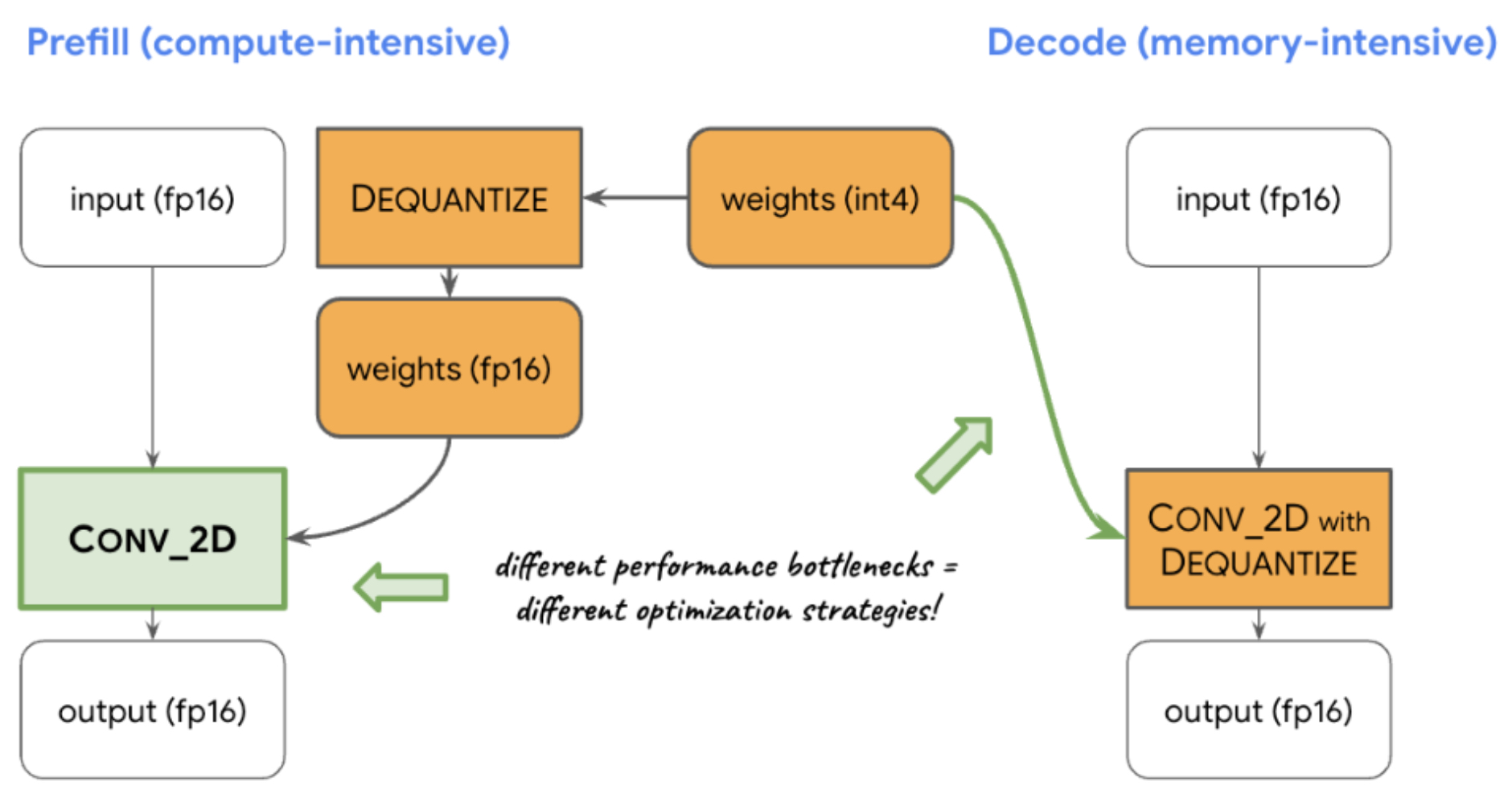
Illustration: Optimizing LLM Inference by Adapting to Compute and Memory Bottlenecks (Different Performance Bottlenecks require Different Optimization Strategies):
- The figure below (source) demonstrates how different performance bottlenecks in the LLM inference pipeline lead to distinct optimization strategies for handling dequantization of weights.
-
In the prefill phase, which is compute-intensive, the model first dequantizes low-bit weights (
int4) into floating-point (float16) values before passing them to the convolution (Conv_2D) operator. This ensures optimal performance for heavy computations, as the floating-point operations run more efficiently on modern processors. -
In contrast, the decode phase is memory-intensive. Here, instead of dequantizing weights ahead of time, the model uses fused Conv_2D with dequantization, keeping weights in their compact form (
int4) until they are needed. This reduces memory bandwidth usage by avoiding unnecessary data expansion during transfer, which is critical when decoding tokens one at a time. -
This design highlights a core principle in system optimization: different stages of computation may require tailored approaches based on their unique constraints—compute-bound stages benefit from early dequantization, while memory-bound stages gain from deferred dequantization.
-
Key takeaways:
-
Performance optimization isn’t one-size-fits-all. You have to understand where the bottleneck is (compute vs memory) and tailor your strategy to the bottleneck:
- Dequantize early when compute-bound (prefill phase).
- Dequantize late when memory-bound (decode phase).
-
This phase-aware optimization is foundational for achieving efficient LLM inference on-device and under constrained compute/memory budgets.
-
Key-Value (KV) Cache Optimization
-
In decoder-based models (e.g., GPT), each new token requires computing self-attention with all past tokens. Without optimization, this scales as:
\[O(n^2 \cdot d)\]- where \(n\) is the number of generated tokens and \(d\) is the hidden dimension.
-
KV cache principle:
- Store the key (K) and value (V) projections for all past tokens during generation.
-
For a new token, compute only its query (Q) and perform:
\[\text{Attention}(Q_t, K_{1:t}, V_{1:t})\] -
This reduces complexity per step to:
\[O(n \cdot d)\]
-
Hardware impact:
- Reduces compute but increases memory bandwidth requirements since past K/V matrices must be accessed repeatedly.
- Critical for CPU-based decoding; also essential on NPUs with limited memory.
-
A detailed discourse on this topic is available in our Model Acceleration primer.
Speculative Decoding
-
Speculative decoding improves throughput by parallelizing token generation while maintaining correctness.
-
Workflow:
- Use a small draft model to propose multiple tokens ahead.
- A larger target model validates or rejects the proposed tokens in parallel.
- Accepted tokens are appended to the sequence; rejected tokens trigger fallback to standard autoregressive decoding.
-
Benefit:
- Reduces total number of sequential steps for the large model.
- Best suited for GPU or NPU where batched verification of tokens can be parallelized.
-
A detailed discourse on this topic is available in our Speculative Decoding primer.
Quantization (4/8-bit)
-
Quantization reduces model weights and activations from
float32orfloat16to lower precision (e.g.,int8orint4).- Static Quantization: Precompute scale factors during calibration on a representative dataset.
- Dynamic Quantization: Scales are computed on-the-fly during inference, less accurate but easier to apply.
-
Equation:
\[x_{quant} = \text{round}\left(\frac{x}{s}\right)\]- where \(s\) is the scaling factor.
-
Benefits:
- Reduces memory footprint by 4–8x.
- Increases throughput on CPUs (via AVX512/AMX) and NPUs (native
int8support).
-
Trade-offs:
- May reduce accuracy, especially for attention layers and small models.
- Requires per-channel quantization for best results.
-
A detailed discourse on this topic is available in our Model Compression primer.
Knowledge Distillation
-
Use a large, accurate teacher model to train a smaller student model:
-
Objective function includes both hard labels and soft probabilities:
\[L = \alpha L_{\text{CE}} + (1 - \alpha) \, \text{KL}(p_{\text{teacher}} \| p_{\text{student}})\] -
Benefit:
- Student model retains much of the teacher’s performance with fewer parameters.
- Ideal for NPUs and CPU edge deployments.
-
A detailed discourse on this topic is available in our Model Compression primer.
Weight Pruning and Low-Rank Approximations
- Pruning removes less important weights (e.g., structured pruning of entire attention heads).
-
Low-rank factorization decomposes weight matrices:
\[W \in \mathbb{R}^{d \times d} \approx U V^T\]- with \(U, V \in \mathbb{R}^{d \times r}, r \ll d\).
-
These reduce both memory and FLOPs.
- A detailed discourse on this topic is available in our Model Compression primer.
Operator and Graph Fusion
- Merge operations like Linear + Bias + LayerNorm to reduce memory reads/writes.
- Frameworks: TensorRT (GPU), OpenVINO (CPU), CoreML (NPU).
Sequence Length and Batch Optimizations
- Use sliding window attention for long sequences.
- Tune batch size to match hardware occupancy (especially on GPUs).
Hardware-Specific Optimization Notes
- CPU: Quantization (
int8), operator fusion, KV caching. - GPU: Mixed precision (
float16/bfloat16), speculative decoding, batching. - TPU: XLA graph compilation, dense matmul optimizations.
- NPU: Static quantization (
int8/int4), model distillation, pruning.
Practical Considerations and Pitfalls When Deploying Transformers on CPU, GPU, and NPUs
- Deploying Transformer models involves multiple trade-offs, particularly around latency, throughput, memory usage, and hardware constraints. This section outlines the key considerations and common pitfalls when working with CPUs, GPUs, and NPUs.
CPU Deployment Considerations
Key Strengths
- General-purpose flexibility
- No need for specialized drivers or runtime
- Lower memory bandwidth than accelerators, but with good cache locality
Watch Out For
-
MatMul Bottlenecks:
- Transformer layers involve large GEMMs (General Matrix-Matrix Multiplications).
- Use libraries like Intel MKL-DNN, oneDNN, or OpenBLAS with AVX2/AVX512 instructions.
-
Cache Contention:
- KV cache can overflow L2/L3 caches, especially with long sequences.
- Performance drops significantly when cache locality is lost.
-
Thread Over-subscription:
- Avoid naive use of multithreading; prefer thread pools and NUMA-aware scheduling.
- Profile using
perf, Intel VTune, or similar tools.
-
Memory Bandwidth:
- CPUs often become memory-bound during decoder operation.
- Optimize memory access patterns and fuse operations to reduce intermediary transfers.
-
Quantization Challenges:
int8quantization is highly effective, but requires calibration and may degrade attention accuracy.- Use dynamic quantization only if static is not viable.
GPU Deployment Considerations
Key Strengths
- Ideal for batched operations and compute-heavy encoder layers
- High memory bandwidth, many-core architecture
Watch Out For
-
Underutilization During Decoding:
- Single-token decode workloads don’t fully occupy GPU cores.
- Consider batching requests or speculative decoding to improve efficiency.
-
Kernel Launch Overhead:
- GPU launch latency can dominate runtime in step-by-step decoding.
- Use fused kernels and persistent caches.
-
Host-Device Memory Transfers:
- Frequent CPU-GPU synchronization (especially during dynamic decoding) can be costly.
- Minimize PCIe transfers and pre-load inputs onto device.
-
Precision Handling:
- Use
float16orbfloat16for faster inference, but be cautious of numerical stability. - Validate that quantized weights preserve generation quality.
- Use
-
Maximize Tensor Core Use:
- Use NVIDIA’s cuBLAS, cuDNN, or FasterTransformer for optimized linear algebra.
TPU Deployment Considerations
Key Strengths
- Extremely efficient for matrix operations
- Suitable for large-batch inference and training
Watch Out For
-
Poor Fit for Decoding:
- TPUs struggle with dynamic token-wise decoding due to fixed compute graph.
- May need to run decode loop on CPU or use alternative methods (e.g., GSPMD)
-
Static Shape Requirements:
- Input/output shapes often must be known ahead of time.
- Makes dynamic batching and long-sequence handling difficult.
-
Limited Ecosystem:
- XLA and TensorFlow/JAX integration are essential.
- Less flexibility than PyTorch or ONNX-based deployments.
NPU Deployment Considerations (Edge/SoC Devices)
Key Strengths
- Extremely efficient for low-power inference
- On-chip memory reduces latency
Watch Out For
-
Operator Support Limitations:
- Custom or unsupported operations must fall back to CPU, drastically hurting performance.
- Stay within the vendor’s supported op-set (e.g., for Apple ANE, Qualcomm Hexagon, etc.).
-
Model Size Constraints:
- Total model size must fit within NPU’s SRAM or limited DRAM window.
- Quantization (
int8orint4) is non-negotiable for many NPUs.
-
Toolchain Lock-in:
- Conversion pipelines (e.g., PyTorch \(\rightarrow\) ONNX \(\rightarrow\) CoreML) must be strictly validated.
- Vendor SDKs may lack transparency and debugging tools.
-
No Runtime Reallocation:
- Static allocation of KV cache, input tensors, and batch sizes is often required.
- This can lead to fragmentation or wasted space.
Summary Table: Key Pitfalls by Hardware
| Platform | Key Pitfall | Best Practices |
|---|---|---|
| CPU | Memory-bound decode + small caches | Use quantization, cache-friendly layouts |
| GPU | Underutilized during decoding | Use batching, speculative decoding, fused kernels |
| TPU | Poor step-by-step token generation | Offload decode to CPU or use static batching |
| NPU | Operator and memory constraints | Quantize, simplify architecture, preallocate buffers |
Parameter Choices and Their Runtime Implications in Transformer Architectures
-
Transformer models have a rich set of architectural parameters — from vocabulary size \(V\) and embedding dimension \(d_{\text{model}}\) to model depth \(L\) and sequence length \(n\) — each influencing runtime in distinct ways. Unlike hyperparameters such as temperature, which affect only sampling behavior, these core architectural choices alter the size of the computational graph, the amount of data moved through memory, and the number of sequential operations per token.
-
Understanding their effects is essential for designing efficient deployments across environments. On GPU-powered servers, parameters can be tuned primarily for accuracy and scale, leveraging high parallelism and bandwidth to absorb their computational cost. On CPUs and NPUs, however, these same choices can make the difference between real-time inference and unusable latency.
-
Each section breaks down a specific parameter or combination of parameters by examining how each major parameter affects:
- Throughput during prefill and decode phases.
- Latency per generated token.
- Memory footprint and cache behavior.
- Energy efficiency for mobile and embedded hardware.
-
The goal behind this section is to offer a practical map for navigating accuracy–latency tradeoffs in any target environment — whether server-class (NanoGPT, TensorRT-LLM, vLLM, DeepSpeed-Inference), on-device/edge CPU (
llama.cpp, GGML, ONNX Runtime), or edge NPU (LidarTLM, MediaPipe + TFLite, Qualcomm SNPE) deployments.
Tokenizer and Vocabulary Size
- A tokenizer converts raw text into discrete tokens that the model can process. The vocabulary size, denoted as \(V\), represents the number of unique tokens the model can recognize. This parameter has several direct and indirect effects on transformer runtime.
Impact on Embedding and Output Layers
-
The embedding layer maps each token ID to a vector of size \(d_{\text{model}}\) (the embedding dimension). The computational and memory cost of this layer is:
- Parameter count: \(P_{\text{embed}} = V \times d_{\text{model}}\)
- Memory footprint: Proportional to \(P_{\text{embed}}\), typically stored in float16 or int8.
- Runtime: At inference, the lookup cost is \(O(1)\) per token, but the softmax in the output layer is \(O(V)\) per token.
-
The largest runtime penalty from a bigger vocabulary comes from the output projection and softmax. The final logits are computed via:
\[z_t = W_{\text{out}} h_t + b\]- where \(W_{\text{out}} \in \mathbb{R}^{V \times d_{\text{model}}}\).
-
This operation costs \(O(V \cdot d_{\text{model}})\) per decoding step. For large \(V\) (e.g., 50k+), this can dominate single-token decode latency on CPUs or NPUs, especially when \(V\) exceeds cache size.
Tradeoffs of Vocabulary Size
-
Larger \(V\)
- Pros: Fewer tokens per sentence (shorter sequences), potentially better language coverage.
- Cons: Larger embedding and output layers, higher per-step cost, more memory bandwidth pressure.
-
Smaller \(V\)
- Pros: Smaller parameter count, faster output projection, better fit for on-device constraints.
- Cons: Longer sequences (more decoding steps), higher total attention cost \(O(n^2 \cdot d)\) in prefill.
-
There is a non-trivial sweet spot where the cost of the output softmax balances with the cost of processing longer sequences.
Runtime Context: Temperature vs. Vocabulary Size
-
Note that temperature (as it relates to decoder sampling) affects randomness and diversity of outputs, but does not impact FLOPs, memory bandwidth, or parameter count. In contrast, vocabulary size directly changes the computational graph and memory access pattern at every generation step.
-
So in terms of runtime importance:
- Vocabulary size is far more significant than temperature for performance.
- Temperature can be tuned freely without runtime cost, but vocabulary size needs to be fixed at training time.
Server vs. On-Device Considerations
-
Server-side (NanoGPT, TensorRT-LLM, vLLM, DeepSpeed-Inference): Large vocabularies are more tolerable since GPUs offer high-bandwidth memory (HBM) and Tensor Cores, which accelerate matrix-vector multiplies in the output layer. Softmax can be fused and batched.
-
On-device (
llama.cpp, LidarTLM, GGML, MediaPipe + TFLite, ONNX Runtime Mobile): Vocabulary size is a primary bottleneck, especially for NPUs or CPUs without fast GEMM acceleration for large matrices. LidarTLM, optimized for edge LiDAR transformers, often uses reduced vocabularies or subword schemes to minimize per-step cost.
Runtime-Specific Notes
-
NanoGPT: Tends toward larger vocab (10–50k), fine for servers but not optimal for low-latency mobile inference.
-
TensorRT-LLM: Optimized for NVIDIA GPUs with fused kernels and mixed-precision GEMMs, allowing large vocab sizes with minimal per-token penalty, especially when batching is used.
-
vLLM: Uses advanced caching and continuous batching strategies on servers, mitigating large-vocab output projection costs, but still sees latency increases at very high \(V\).
-
llama.cpp: Often run quantized on CPUs; vocab size affects KV cache read/write less than it affects output projection latency. Implements vocabulary lookups and output projection via cache-aware tiled GEMM in GGML to minimize L3 cache misses. -
LidarTLM: Frequently aggressively pruned vocab for ultra-low-power environments.
-
MediaPipe + TFLite LLMs: For mobile/embedded devices, vocab size is often cut down to 4k–8k to meet NPU SRAM limits, with aggressive quantization applied to the embedding and projection layers.
-
ONNX Runtime (CPU/NPU): On CPU, large vocabularies can cause cache misses in the output projection; on NPU, unsupported large matrix ops may be forced to fall back to CPU, severely impacting latency.
Model/Embedding Dimension
- The model dimension (also called the “embedding dimension”), \(d_{\text{model}}\), determines the dimensionality of token embeddings and hidden states across the transformer.
- The model dimension has a direct, predictable effect on runtime cost. Increasing the model dimension even slightly can push an on-device model from real-time to unusably slow since it appears in nearly every computational term in the architecture.
Where the Model Dimension Shows Up
- Embedding Layer:
- Parameter count:
- Memory bandwidth scales linearly with \(d_{\text{model}}\) when loading embeddings.
- Multi-Head Attention (MHA):
- Each attention projection (\(Q, K, V,\) output) is a matrix multiply of shape \((n \times d_{\text{model}}) \times (d_{\text{model}} \times d_{\text{proj}})\).
- FLOPs per layer for MHA (excluding softmax):
- Since \(d_{\text{head}} \cdot h = d_{\text{model}}\), the cost scales as \(O(n^2 \cdot d_{\text{model}})\) for attention scores and \(O(n \cdot d_{\text{model}}^2)\) for projections.
- Feedforward Network (FFN):
- Uses intermediate size \(d_{\text{ff}} \approx 4 \cdot d_{\text{model}}\).
- Per layer FLOPs:
-
Output Projection:
\[O(V \cdot d_{\text{model}})\]- This is where \(d_{\text{model}}\) multiplies with vocab size effects (cf. Tokenizer and Vocabulary Size section).
Impact on the KV Cache
-
Increasing the model/embedding dimension \(d_{\text{model}}\) linearly increases the size of the KV cache, which stores past attention states, and can quickly become a major driver of memory usage during inference.
-
During inference, each attention layer stores the Key (\(K\)) and Value (\(V\)) projections for every processed token in a KV cache, allowing the model to reuse past context without recomputing attention.
-
For a model with \(h\) heads, head dimension \(d_{\text{head}}\), and embedding dimension \(d_{\text{model}} = h \cdot d_{\text{head}}\), the KV cache size per token for a single layer is:
\[\text{KV size per token} = 2 \times d_{\text{model}}\]- where, the factor of 2 accounts for storing both \(K\) and \(V\).
-
For a sequence of length \(n\) and \(L\) transformer layers, the total KV cache size is:
\[\text{Total KV memory} = L \times n \times 2 \times d_{\text{model}} \times \text{sizeof(dtype)}\] -
Why this grows with \(d_{\text{model}}\):
- Both \(K\) and \(V\) vectors have dimensionality \(d_{\text{model}}\), so increasing \(d_{\text{model}}\) directly increases the number of stored values per token.
- The growth is linear with respect to \(d_{\text{model}}\), but multiplicative with \(n\) and \(L\).
- This means that even modest increases in \(d_{\text{model}}\) can cause large jumps in memory usage for long sequences or deep networks.
-
Practical implications:
- Larger \(d_{\text{model}}\) means more memory bandwidth required to read/write the KV cache, which can bottleneck inference.
- On memory-limited devices, KV cache capacity often becomes the limiting factor before compute throughput does.
Runtime and Memory Effects
-
Larger Model Dimension:
- Pros: More capacity per token, better representation quality, higher perplexity performance.
- Cons: Quadratic or linear increase in FLOPs for most layers, large memory footprint, higher activation size in KV cache.
-
Smaller Model Dimension:
- Pros: Smaller models, faster inference, better suited for edge devices.
- Cons: Lower expressive power; can bottleneck performance before parameter count is reached.
Interaction with Sequence Length
- While increasing the model dimension linearly scales memory and compute in most layers, attention score calculation (\(O(n^2 \cdot d_{\text{model}})\)) means that with long sequences, the impact of \(d_{\text{model}}\) is amplified.
Server vs. On-Device
- Server (NanoGPT, TensorRT-LLM, vLLM, DeepSpeed-Inference):
- Can afford larger \(d_{\text{model}}\) (e.g., 2048+) due to GPU tensor cores and high-bandwidth memory. The main tradeoff is training/inference cost, not latency.
- TensorRT-LLM uses fused attention kernels and mixed-precision GEMMs to sustain high throughput at large \(d_{\text{model}}\), while vLLM and DeepSpeed-Inference can overlap compute and memory ops to mask latency.
- On-Device (llama.cpp, GGML, ONNX Runtime Mobile):
- \(d_{\text{model}}\) needs to be small enough to fit activations and KV cache in available RAM/LLC. Even quantized models struggle if \(d_{\text{model}}\) > 1024 on low-end CPUs.
llama.cppand GGML use block-quantized matrix multiplies to reduce memory footprint, while ONNX Runtime Mobile leverages kernel fusion for small \(d_{\text{model}}\) efficiency.
- Edge-specialized (LidarTLM, MediaPipe + TFLite, Qualcomm AI Stack):
- Often uses \(d_{\text{model}}\) = 256–512 for real-time inference in sensor fusion pipelines, balancing compute with strict power envelopes.
- MediaPipe + TFLite models targeting NPUs frequently compress \(d_{\text{model}}\) to fit SRAM, while the Qualcomm AI Stack uses
int8/float16hybrid kernels to keep latency under frame-time budgets.
Sequence Length and KV Cache Size
- The sequence length \(n\) (number of tokens in context) directly controls both the prefill phase cost and the decode phase memory demands in transformer inference.
- Sequence length has a relatively large runtime impact since it changes the size of the entire compute graph and KV cache footprint.
Computational Scaling
- Prefill (parallelizable):
- Multi-head attention complexity for the encoder or decoder prefill step:
- Because all \(n\) tokens attend to all others, cost grows quadratically. Increasing sequence length from 2k to 4k tokens quadruples the attention score computation.
- Decode (autoregressive):
- With KV caching, each new token attends to all past tokens:
- This is linear per token, but multiplied across \(n_{\text{gen}}\) output tokens.
KV Cache Size and Memory Footprint
-
In autoregressive decoding, the KV cache stores keys and values for each token at each layer:
\[KV_{size} \approx n \times L \times 2 \times d_{\text{model}} \times \text{precision}\]-
where:
- \(n\): sequence length so far
- \(L\): number of layers
- Factor 2: separate \(K\) and \(V\) storage
- precision: bytes per element (e.g., 2 for
float16, 1 for int8)
-
-
Example: For \(n = 2048, L = 24, d_{\text{model}} = 1024,\)
float16, KV cache ≈ 192 MB.
Latency Effects
- Prefill latency dominated by large GEMMs (matrix multiplications) \(\rightarrow\) compute-bound.
- Decode latency dominated by KV cache reads and output projection \(\rightarrow\) memory-bound.
-
Large \(n\) increases both phases:
- In prefill: longer sequences multiply the quadratic term.
- In decode: KV cache memory footprint grows, possibly exceeding L2/L3 cache \(\rightarrow\) slower fetches.
Server vs. On-Device
- Server (NanoGPT, TensorRT-LLM, vLLM, DeepSpeed-Inference):
- GPUs can handle long sequences for prefill, but decode can still be underutilized unless batching or speculative decoding is applied. KV cache often fits in GPU memory without issue.
- TensorRT-LLM and DeepSpeed-Inference use fused attention kernels to reduce KV cache memory bandwidth costs, while vLLM leverages continuous batching to mask decode-phase stalls.
- On-Device (
llama.cpp, GGML, ONNX Runtime Mobile):- Sequence length is often capped (e.g., 512–1024 tokens) to avoid RAM exhaustion and to keep KV cache in CPU last-level cache. Even at
int8quantization, longer contexts can stall inference. llama.cppand GGML implement tiled KV cache layouts to keep hot data in L3 cache; ONNX Runtime Mobile sometimes offloads KV cache to DRAM when SRAM is insufficient, impacting latency.
- Sequence length is often capped (e.g., 512–1024 tokens) to avoid RAM exhaustion and to keep KV cache in CPU last-level cache. Even at
- Edge-specialized (LidarTLM, MediaPipe + TFLite LLMs):
- Sequences are kept short (e.g., 128–256 tokens) because LiDAR frame-based context naturally fits into smaller windows, allowing real-time inference.
- On TFLite NPUs, static allocation of KV cache in SRAM ensures deterministic performance and avoids runtime allocation delays.
Parameter Count and Model Depth
- The total parameter count \(P\) and model depth \(L\) (number of transformer blocks) determine the model’s representational capacity and directly affect runtime.
- Doubling \(L\) roughly doubles per-token latency.
Parameter Count Decomposition
-
A rough parameter breakdown for a decoder-only transformer:
-
Embedding matrices:
\[P_{\text{embed}} = V \cdot d_{\text{model}}\] -
Per-layer parameters:
-
Attention projections (\(Q\), \(K\), \(V\), \(O\)):
\[4 \cdot d_{\text{model}}^2\] -
Feedforward networks:
\[2 \cdot d_{\text{model}} \cdot d_{\text{ff}} \approx 8 \cdot d_{\text{model}}^2\] -
LayerNorm & biases: negligible in size
-
-
Total model parameters:
\[P_{\text{total}} \approx P_{\text{embed}} + L \cdot (12 \cdot d_{\text{model}}^2)\]
-
-
This shows that increasing depth \(L\) linearly scales parameter count and compute cost, whereas increasing \(d_{\text{model}}\) scales cost quadratically.
Runtime Scaling with Depth
- Prefill phase: Cost scales as \(O(L \cdot n^2 \cdot d_{\text{model}}) \quad \text{(attention)}\) plus \(O(L \cdot n \cdot d_{\text{model}}^2) \quad \text{(FFN)}\).
- Decode phase: Each new token must pass through all \(L\) layers sequentially, so latency per token scales linearly with \(L\).
Accuracy vs. Latency Tradeoff
- More layers generally yield better performance and longer-range reasoning, but each layer adds sequential compute steps during decoding.
- Shallow networks are much faster for autoregressive decoding but can struggle with complex reasoning or long-range dependencies.
Server vs. On-Device
-
Server (NanoGPT, TensorRT-LLM, vLLM, DeepSpeed-Inference): Large \(L\) (24–48) is feasible. GPUs can hide some latency through parallelization across layers with pipeline or tensor parallelism. The prefill stage dominates for long contexts.
-
On-Device (
llama.cpp, GGML, ONNX Runtime Mobile): Depth often limited to 8–16 layers for real-time inference. Too many layers \(\rightarrow\) sequential decode bottleneck on CPU or NPU. Quantization helps memory but not sequential compute cost. -
Edge-specialized (LidarTLM, MediaPipe + TFLite LLMs): Extremely shallow depths (4–8 layers) to maintain low latency for sensor-fusion loops. Accuracy loss offset by task-specific training and limited context size.
Embedding Size \(\times\) Vocabulary Size \(\times\) Depth
- So far, we’ve treated vocabulary size \(V\), embedding size \(d_{\text{model}}\), and depth \(L\) mostly in isolation. In reality, these parameters interact in ways that compound runtime and memory demands.
Compound Parameter Scaling
- By examining the compute vs. memory analysis for tokenizer and vocabulary size, model/embedding size \(d_{model}\), sequence length and KV cache size, and model parameter count and depth \(L\), a decoder-only transformer’s core parameter count is approximately:
- The output projection cost per token is:
-
The layer cost per token is:
- \[C_{\text{layer}} \approx O(L \cdot d_{\text{model}}^2)\]
-
This implies:
- Increasing \(d_{\text{model}}\) scales both terms quadratically (via layers) and linearly (via vocab projection).
- Increasing \(V\) scales only the embedding/output projection term, but that term appears every decoding step.
- Increasing \(L\) increases sequential operations per token, which is critical for autoregressive decoding latency.
Interactions in Practice
- Large \(V\) + Large \(d_{\text{model}}\): Output projection dominates decode latency, especially on memory-bound devices.
- Large \(L\) + Long Sequence \(n\): Prefill becomes a quadratic wall due to attention; decode slows due to sequential depth.
- Small \(V\) + Small \(d_{\text{model}}\) + Moderate \(L\): Often the sweet spot for edge devices — balanced compute and memory, but can sacrifice accuracy.
Optimization Strategies by Deployment Context
-
Server (NanoGPT, TensorRT-LLM, vLLM, DeepSpeed-Inference):
- High \(V\), high \(d_{\text{model}}\), large \(L\) are fine if GPUs are saturated.
- Use fused output softmax kernels and half-precision Tensor Core paths.
- Speculative decoding helps mitigate large \(L\) in decode.
-
On-Device CPU (
llama.cpp, GGML, ONNX Runtime Mobile):- Reduce \(V\) aggressively to cut output projection cost.
- Moderate \(d_{\text{model}}\) (512–1024) to keep KV cache and GEMMs manageable.
- Lower \(L\) to speed sequential decode; apply quantization (
int8/int4) to fit in RAM.
-
Edge NPU (LidarTLM, MediaPipe + TFLite LLMs, Qualcomm AI Engine Direct):
- Task-specific \(V\) (often <10k) to minimize projection latency.
- Small \(d_{\text{model}}\) (256–512) for throughput under strict power budgets.
- Shallow \(L\) (4–8) to ensure deterministic real-time latency for sensor fusion loops.
Tradeoffs
- Reducing \(V\) trades fewer softmax FLOPs for longer token sequences (more steps).
- Reducing \(d_{\text{model}}\) cuts compute cost per layer but reduces representation power.
- Reducing \(L\) cuts sequential latency but lowers reasoning depth and long-context handling.
Parameter Tuning Recipes for ML Runtimes
- This section distills the relationships between vocabulary size \(V\), embedding size \(d_{\text{model}}\), and depth \(L\) into actionable configurations, balancing accuracy, latency, and memory for three representative environments.
NanoGPT (Server Inference / GPU-centric)
- Hardware Context: High-bandwidth memory (HBM), tensor cores, strong batched throughput.
-
Parameter Priorities:
- Large \(V\) (30k–50k) acceptable due to fused softmax and fast GEMM kernels.
- High \(d_{\text{model}}\) (1536–2048) to maximize model capacity.
- Deep \(L\) (24–48) for reasoning and long-context tasks.
-
Typical Config:
\[V = 50{,}000, \quad d_{\text{model}} = 2048, \quad L = 36, \quad \text{seq len} = 4096\] -
Expected Behavior:
- Prefill dominated by attention FLOPs, but GPUs handle with parallelization.
- Decode latency per token low in absolute terms due to high raw throughput, but still benefits from speculative decoding.
-
Optimization Levers:
- Mixed precision (
float16/bfloat16). - Layer fusion (e.g., FasterTransformer).
- Batch multiple decode streams to utilize GPU fully.
- Mixed precision (
vLLM (Server Inference / GPU-centric)
- Hardware Context: GPU servers optimized for dynamic batching.
-
Parameter Priorities:
- Large \(V\) acceptable with efficient memory layouts.
- High \(d_{\text{model}}\) paired with aggressive continuous batching.
- Depth \(L\) tuned for target latency vs throughput.
-
Optimization Levers:
- Continuous batching to keep GPU fully utilized.
- KV cache sharing across requests.
TensorRT-LLM (Server Inference / GPU-centric)
- Hardware Context: NVIDIA GPUs with Tensor Cores and high-bandwidth memory.
-
Parameter Priorities:
- Large \(V\) (up to 100k) supported with minimal softmax overhead via fused kernels.
- High \(d_{\text{model}}\) (up to 4096) leveraged for accuracy without extreme latency.
- Moderate-to-deep \(L\) (20–48) manageable due to high parallelism.
-
Typical Config:
\[V = 80{,}000, \quad d_{\text{model}} = 3072, \quad L = 40, \quad \text{seq len} = 8192\] -
Optimization Levers:
- Tensor Core–optimized mixed-precision GEMM.
- Fused attention and output projection.
llama.cpp (On-Device Inference / CPU-centric)
- Hardware Context: Commodity x86/ARM CPU, limited parallelism, cache-sensitive.
-
Parameter Priorities:
- Reduce \(V\) (16k–32k) to keep output projection matrix small and cache-friendly.
- Moderate \(d_{\text{model}}\) (512–1024) to keep KV cache within LLC.
- Lower \(L\) (8–16) to reduce sequential decode steps.
-
Typical Config:
\[V = 32{,}000, \quad d_{\text{model}} = 768, \quad L = 12, \quad \text{seq len} = 1024\] -
Expected Behavior:
- Prefill latency noticeable with large \(n\), but acceptable for short prompts.
- Decode speed highly sensitive to \(L\)% and KV cache fit.
-
Optimization Levers:
- int8/int4 quantization.
- Operator fusion (ONNX Runtime, GGML backend).
- Cache-aware layout for KV storage.
LidarTLM (Edge NPU / Sensor Fusion)
- Hardware Context: Mobile/embedded NPU with strict SRAM and thermal limits.
-
Parameter Priorities:
- Task-specific \(V\) (4k–10k) to minimize projection latency.
- Small \(d_{\text{model}}\) (256–512) for real-time throughput.
- Shallow \(L\) (4–8) for deterministic frame-to-frame latency.
-
Typical Config:
\[V = 8{,}000, \quad d_{\text{model}} = 384, \quad L = 6, \quad \text{seq len} = 256\] -
Expected Behavior:
- Prefill and decode both complete well within a LiDAR frame budget (~33 ms).
- KV cache fits entirely in on-chip SRAM, avoiding DRAM latency.
-
Optimization Levers:
- Static
int8quantization. - Operator fusion tailored to NPU’s op-set.
- Preallocation of all buffers to avoid runtime allocation overhead.
- Static
MediaPipe + TFLite LLMs (Mobile/Edge Inference / Specialized IPs such as NPUs/DSPs)
- Hardware Context: Smartphone SoCs with NPUs/DSPs.
-
Parameter Priorities:
- Reduced \(V\) (4k–8k) to fit projection in SRAM.
- Small \(d_{\text{model}}\) (256–512) to fit memory and meet latency budgets.
- Shallow \(L\) for real-time responses.
-
Optimization Levers:
- Fully quantized static graphs.
- Operator fusion for NPU op-sets.
Cross-Platform Insights
- Large \(V\): Fine on GPU servers, problematic for CPU/NPU without GEMM acceleration.
- Large \(d_{\text{model}}\): Improves accuracy but hurts both memory and compute — only viable if hardware bandwidth is high.
- Large \(L\): Boosts reasoning but increases decode latency linearly — worst-case for low-parallelism CPUs.
- Temperature: Has zero impact on runtime — safe to tune purely for output diversity.
References
- Efficient Inference with Transformer Models on CPUs
- Speculative Decoding for Accelerated Transformer Inference
- Fast Transformers with Memory-Efficient Attention via KV Cache Optimization
- SmoothQuant: Accurate and Efficient Post-Training Quantization for Large Language Models
- Intel Extension for PyTorch: Boosting Transformer Inference on CPUs
- FasterTransformer GitHub Repository (NVIDIA)
- vLLM: Easy and Fast LLM Serving with State-of-the-Art Throughput
- Deploying Transformer Models on Edge Devices with TensorRT
- Quantization Aware Training in PyTorch
- ONNX Runtime: Accelerating Transformer Inference
- Speculative Decoding in vLLM (Medium article)
- Running LLMs on Mobile: Lessons from Distilling and Quantizing GPT-2
- Optimizing LLM Serving on NVIDIA GPUs with TensorRT-LLM
- LLM INT4 Inference with ONNX Runtime
- Efficient Transformer Inference on Edge with EdgeTPU
- Large Language Models On-Device with MediaPipe and TensorFlow Lite
Citation
If you found our work useful, please cite it as:
@article{Chadha2020DistilledOnDeviceTransformers,
  title   = {On-device Transformers},
  author  = {Chadha, Aman},
  journal = {Distilled AI},
  year    = {2020},
  note    = {\url{https://aman.ai}}
}