Primers • Model Compression for On-Device AI
- Background
- Overview
- Quantization
- Background: Precision
- Background: Matrix Multiplication in GPUs
- Definition
- Types of Quantization
- Dequantization Considerations
- Quantization Workflows
- Benefits and Limitations
- Mitigation Strategies
- Weights vs. Activation Quantization
- Quantization with PyTorch
- Comparative Analysis
- Compute vs. Memory Bottlenecks
- Modern Quantization Techniques
- GPTQ: Quantization with Second-Order Error Compensation
- SmoothQuant
- Activation-Aware Weight Quantization (AWQ)
- GGUF Quantization (Legacy, K‑Quants, I‑Quants)
- AWEQ: Activation‑Weight Equalization
- EXL2 Quantization
- SpinQuant
- FPTQuant
- Palettization (Weight Clustering)
- What to Use When?
- Comparative Analysis
- Multimodal Quantization
- Why VLM Quantization Is More Complex
- Quantizing the Visual Backbone
- Quantizing the Language Backbone
- Cross-Modal Projection and Fusion Layer Quantization
- Quantization-Aware Training (QAT) in VLMs
- Calibration and Evaluation in VLMs
- Hybrid and Mixed-Precision Quantization
- Tooling Support
- Comparative Analysis of LLMs vs. VLM Quantization
- Device and Operator Support across Frameworks
- Choosing the right quantization approach
- Performance Results
- Accuracy results
- Popular Quantization Libraries
- How Far Can Quantization Be Pushed?
- Further Reading
- Knowledge Distillation
- Mechanism
- Types of Knowledge Distillation
- Distillation Modes
- Why Use Knowledge Distillation Instead of Training Small Models from Scratch?
- Why Knowledge Distillation Works
- Distillation in Practice
- Reverse Distillation
- Weak Supervision via Distillation
- Compute vs. Memory Bottlenecks
- Limitations and Challenges
- Model Pruning
- Mixed Precision Training
- Low-Rank Decomposition & Adaptation
- Lightweight Model Design
- What to use When?
- Combining Model Compression Techniques
- Further Reading
- References
- Citation
Background
-
Modern generative models often contain between 100 billion to 1 trillion parameters. Since each parameter (as a 32-bit float) consumes 4 bytes, the memory footprint can scale from 400 GB to over 4 TB. This makes them prohibitively large for deployment on edge devices, where memory and compute resources are highly constrained. Furthermore, deploying machine learning models directly on edge devices such as smartphones, tablets, or embedded systems offers key advantages in privacy, latency, and user experience. On-device processing ensures that data remains local to the device, significantly reducing the risk of exposure from data transmission or centralized storage breaches. This is particularly critical for applications in computer vision and conversational AI, where interactions often involve personal or sensitive information.
-
However, the computational and memory demands of modern machine learning models—especially large language models—pose a major barrier to efficient on-device deployment. These models are typically too large and resource-intensive to run in real-time on devices with limited hardware capabilities. As models continue to scale in size and complexity, challenges such as increased latency, power consumption, and hardware constraints become even more pronounced.
-
To address these limitations, a wide array of model compression and optimization techniques has been developed. These include model quantization (static, dynamic, and quantization-aware training), structured and unstructured pruning, knowledge distillation (response-based, feature-based, relation-based), low-rank decomposition, activation-aware quantization, operator fusion, and mixed precision training. Advanced post-training quantization methods such as AWQ, SmoothQuant, SpinQuant, AWEQ, and FPTQuant further push the boundaries of efficient model deployment.
-
Collectively, these techniques aim to reduce model size, lower computational complexity, and accelerate inference—without significantly compromising accuracy. By enabling smaller, faster, and more power-efficient models, these strategies make it increasingly feasible to run advanced AI applications directly on user devices, supporting both better privacy and smoother user experiences.
Overview
-
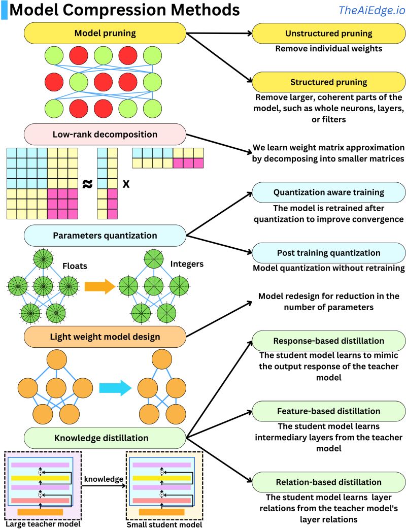
To enable on-device AI, a wide range of model compression techniques have been developed. Below, we visually and conceptually summarize the five core strategies widely used in industry and research.
- Model Quantization
-
Quantization reduces the precision of weights and activations, typically from 32-bit floats to 8-bit integers, yielding up to a 4× reduction in model size and significant speed-ups using optimized kernels.
- Post-training quantization applies precision reduction directly on a trained model and may include heuristic corrections (e.g., bias correction, per-channel scaling).
- Quantization-aware training (QAT) simulates quantization noise during training, allowing the model to adapt and maintain higher accuracy under reduced precision.
- Advanced quantization strategies like AWQ, SmoothQuant, and AWEQ refine post-training quantization by adjusting scaling factors or reweighting attention layers.
- A detailed discourse on this topic is available in the Quantization section.
-
- Knowledge Distillation
-
Knowledge distillation trains a compact student model to mimic a larger teacher model.
- Response-based distillation focuses on matching the output logits or probabilities.
- Feature-based distillation aligns intermediate representations between teacher and student.
- Relation-based distillation preserves inter-feature dependencies (e.g., attention maps).
- Distillation is often combined with other techniques (e.g., quantization or pruning) to maximize efficiency.
- A detailed discourse on this topic is available in the Knowledge Distillation section.
-
- Model Pruning
-
Pruning reduces model size by removing weights that have minimal impact on overall performance.
- Unstructured pruning eliminates individual weights based on their magnitude (e.g., L1/L2 norm) or gradient impact (e.g., first or second derivative of the loss).
- Structured pruning goes further by removing entire neurons, filters, or layers, which can directly lead to faster inference on hardware accelerators.
- In practice, pruning is often iterative: prune, retrain, evaluate, and repeat to recover performance loss.
- A detailed discourse on this topic is available in the Model Pruning section.
-
- Low-Rank Decomposition
-
Many neural networks, especially transformer-based architectures, contain large weight matrices that can be approximated as a product of smaller matrices.
- For example, an N×N matrix can often be replaced by two N×k matrices (with \(k << N\)), reducing space complexity from \(O(N^2)\) to \(O(N \cdot k\)).
- Methods like SVD (singular value decomposition) or CP decomposition are used here.
- In practice, fine-tuning the decomposed model is essential to restore original performance.
- A detailed discourse on this topic is available in the Low-Rank Decomposition section.
-
- Lightweight Model Design
-
Rather than compressing an existing model, lightweight design focuses on creating efficient architectures from the ground up.
- Examples include MobileBERT, DistilBERT, TinyBERT, and ConvNeXt-T, which use smaller embedding sizes, depth-wise separable convolutions, fewer transformer blocks, or other architectural efficiencies.
- Empirical design choices are often guided by NAS (Neural Architecture Search) or latency-aware loss functions.
- A detailed discourse on this topic is available in the Lightweight Model Design section.
-
- The illustration below (source) summarizes how these different compression methods contribute to reducing model size and enabling efficient deployment across platforms, including on-device scenarios.
Quantization
Background: Precision
-
Before diving into quantization, it’s essential to understand precision—specifically, how computers represent decimal numbers like
1.0151or566132.8. Since we can conceive of infinitely precise values (like π), but only have limited space in memory, there’s a fundamental trade-off between precision (how many significant digits can be stored) and size (how many bits are used to represent the number). -
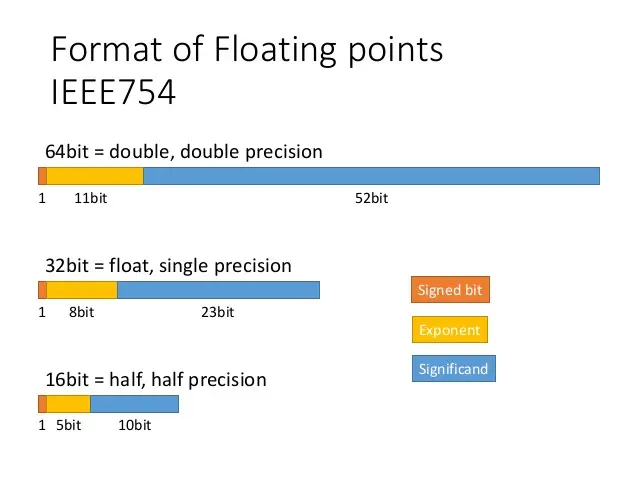
In computer engineering, these values are stored as floating point numbers, governed by the IEEE 754 floating point standard. This specification defines how bits are allocated to represent the sign, exponent, and mantissa (also called the significand, which holds the meaningful digits).
-
Floating point formats vary by their bit-width, and each level of precision has a different rounding error margin:
- Double-precision (
fp64) – 64 bits, max rounding error of approximately \(2^{-52}\). - Single-precision (
float32) – 32 bits, max rounding error of approximately \(2^{-23}\). - Half-precision (
float16) – 16 bits, max rounding error of approximately \(2^{-10}\).
- Double-precision (
-
For a deeper exploration, check out the PyCon 2019 talk: “Floats are Friends: making the most of IEEE754.00000000000000002”.
-
In practice:
- Python defaults to using
fp64for itsfloattype. - PyTorch, which is optimized for performance and memory efficiency, defaults to
float32.
- Python defaults to using
-
Understanding these formats is crucial when moving on to concepts like mixed precision training, where models leverage different floating point types to balance performance and accuracy.
-
Maarten Grootendorst’s A Visual Guide to Quantization offers a visuals to help you develop an intuition about the methodologies, use cases, and the principles behind quantization.
IEEE 754 Floating Point Standard
-
The IEEE 754 standard defines the binary representation of floating point numbers used in nearly all modern hardware and programming environments. A floating-point number is composed of three parts:
- Sign bit (\(S\)): 1 bit indicating positive or negative.
- Exponent (\(E\)): Encodes the range (scale) of the number.
- Mantissa or significand (\(M\)): Encodes the precision.
-
The general representation for a binary floating-point number is:
-
Each format—half, single, and double—allocates a different number of bits to these components, balancing precision and range against memory usage and compute requirements.
-
The following figure (source) shows the IEEE 754 standard formats for floating-point numbers, illustrating the bitwise layout of the signed bit, exponent, and significand across double (64-bit), single (32-bit), and half (16-bit) precision representations.
Half-Precision (float16)
- Bit layout: 1 sign bit, 5 exponent bits, 10 mantissa/significand bits.
- Total bits: 16
- Exponent bias: 15
- Dynamic range: Approximately \(6 \times 10^{-5}\) to \(6.5 \times 10^4\)
-
Half-precision is mostly used during inference, especially in low-power or memory-constrained environments such as mobile devices or embedded hardware. It offers limited range and precision, and is generally not suitable for training deep networks unless special care is taken (e.g., using loss scaling or
float32accumulations). -
GPU Considerations:
- Many GPUs, like NVIDIA’s Volta, Turing, Ampere, Hopper, Blackwell, include specialized hardware units called Tensor Cores optimized for
float16operations. float16can be processed at higher throughput thanfloat32, enabling significant speedups for matrix multiplications during inference.- Often paired with Mixed-Precision Training (MPT), where activations and weights are stored in
float16, but gradients are accumulated infloat32.
- Many GPUs, like NVIDIA’s Volta, Turing, Ampere, Hopper, Blackwell, include specialized hardware units called Tensor Cores optimized for
Single-Precision (float32)
- Bit layout: 1 sign bit, 8 exponent bits, 23 mantissa bits.
- Total bits: 32
- Exponent bias: 127
- Dynamic range: Approximately \(1.4 \times 10^{-45}\) to \(3.4 \times 10^{38}\)
-
float32is the default numerical format for most deep learning frameworks and hardware. It provides a good balance between precision and range, making it robust for both training and inference. -
GPU Considerations:
- Supported natively on all modern GPUs.
- Most general-purpose ALUs (Arithmetic Logic Units) on the GPU are designed to process
float32efficiently. - Slower than
float16orbfloat16in terms of throughput and power usage but more accurate.
Double-Precision (float64)
- Bit layout: 1 sign bit, 11 exponent bits, 52 mantissa bits.
- Total bits: 64
- Exponent bias: 1023
- Dynamic range: Approximately \(5 \times 10^{-324}\) to \(1.8 \times 10^{308}\)
float64is typically used in scientific computing, numerical simulations, and applications requiring high precision. It is rarely used in deep learning because its benefits are minimal for most ML tasks, while the compute and memory costs are high.
Brain Floating Point (bfloat16)
- Bit layout: 1 sign bit, 8 exponent bits, 7 mantissa bits
- Total bits: 16
- Exponent bias: 127 (same as
float32) - Dynamic range: Approximately \(1.2 \times 10^{-38}\) to \(3.4 \times 10^{38}\)
-
bfloat16(Brain Floating Point 16) was introduced by Google for training deep neural networks. Unlikefloat16, which reduces both exponent and mantissa bits,bfloat16keeps the same exponent width asfloat32(8 bits) but reduces the mantissa to 7 bits. -
This design retains the dynamic range of
float32, which makes it far more robust to underflow/overflow issues during training compared tofloat16. -
However, the precision is reduced, since fewer mantissa bits mean fewer significant digits are preserved. Despite this, it performs well in practice for training large models.
-
bfloat16is ideal for training tasks where:- High dynamic range is important
- Some loss of precision can be tolerated (e.g., in early layers or gradients)
- Lower memory and compute overhead is desired compared to
float32
-
It is commonly used in mixed-precision training, often with accumulations in
float32to improve numerical stability. -
Use cases:
- Large-scale model training (e.g., LLMs)
- TPUs (Google Cloud), and newer GPUs from NVIDIA, AMD, and Intel that support native
bfloat16ops
GPU/TPU Considerations
-
float16:
- Supported by specialized hardware units (Tensor Cores) in NVIDIA Volta, Turing, Ampere, Hopper, and Blackwell architectures.
- Offers higher throughput and lower memory usage, especially during inference.
- Typically used in mixed-precision training with
float32accumulations to maintain stability.
-
bfloat16:
- Natively supported on Google TPUs, NVIDIA Ampere and newer (e.g., A100, H100), Intel Habana Gaudi accelerators, and select AMD GPUs.
- Enables high dynamic range similar to
float32while halving memory usage. - Increasingly adopted in training large models where
float16may encounter stability issues. - Like
float16,bfloat16is also used in mixed-precision training pipelines.
-
float32:
- Universally supported across all GPU architectures.
- Offers the best balance between range and precision.
- Slower and more memory-intensive compared to
float16andbfloat16.
-
float64:
- Rare in deep learning; primarily used in scientific computing.
- Most GPUs support it at much lower throughput.
- Often omitted entirely from inference workloads due to cost.
Comparative Summary
| Format | Bits | Exponent Bits | Mantissa Bits | Bias | Range (Approx.) | GPU Usage |
|---|---|---|---|---|---|---|
| float16 | 16 | 5 | 10 | 15 | \(10^{-5}\) to \(10^{4}\) | Fast inference, mixed precision |
| bfloat16 | 16 | 8 | 7 | 127 | \(10^{-38}\) to \(10^{38}\) | Training + inference, high range |
| float32 | 32 | 8 | 23 | 127 | \(10^{-45}\) to \(10^{38}\) | Default for training |
| float64 | 64 | 11 | 52 | 1023 | \(10^{-324}\) to \(10^{308}\) | Rare in ML, slow on GPU |
- This foundation in floating point formats prepares us to understand quantization—where bit-widths are reduced even further (e.g., 8-bit, 4-bit, or binary)—to achieve efficient computation with minimal loss in model performance.
Background: Matrix Multiplication in GPUs
-
Efficient matrix multiplication is at the heart of modern deep learning acceleration on GPUs. This section provides a high-level view of how matrix-matrix multiplications are implemented and optimized on GPU hardware, with special focus on tiling, Tensor Cores, and the performance implications of quantization.
-
Matrix multiplications, especially General Matrix Multiplications (GEMMs), are a core computational primitive in deep learning workloads. Whether in fully connected layers, convolutions (via
im2col), or attention mechanisms, these operations are executed billions of times during training and inference. As such, optimizing GEMM performance is essential for efficient neural network execution, particularly on GPUs. -
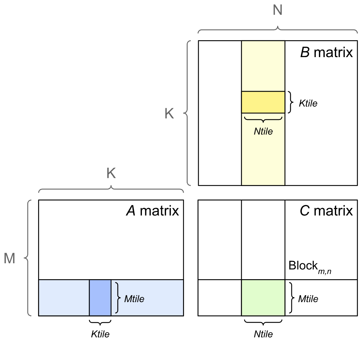
To execute GEMMs efficiently, GPUs partition the output matrix into tiles. Each tile corresponds to a submatrix of the result and is computed by a thread block. The GPU steps through the input matrices along the shared dimension (K) in tiles, performing multiply-accumulate operations and writing the results into the corresponding tile of the output matrix. The illustration below (source) shows the tiled outer product approach to GEMMs.
-
Thread blocks are mapped to the GPU’s streaming multiprocessors (SMs), the fundamental compute units that execute instructions in parallel. Each SM can process one or more thread blocks concurrently, depending on the available resources and occupancy.
-
Performance in GPU matrix multiplication is often bounded by one of two factors:
- Compute (math) bound: When the arithmetic intensity (FLOPs per byte) is high enough that math operations dominate runtime.
- Memory bound: When the operation requires frequent memory access compared to math operations, limiting throughput.
-
Whether a given GEMM is compute- or memory-bound depends on the matrix dimensions (\(M, N, K\)) and the hardware’s characteristics. For example, matrix-vector products (where either \(M\) = 1 or \(N\) = 1) are typically memory-bound due to their low arithmetic intensity.
-
Modern NVIDIA GPUs include specialized hardware units called Tensor Cores, which are designed to accelerate GEMMs involving low-precision data types such as
float16,bfloat16, andint8. Tensor Cores perform small matrix multiplications in parallel and require that the matrices’ dimensions align with certain multiples (e.g., 8 forfloat16, 16 forint8) to achieve peak performance. For instance, on Ampere and newer architectures like Hopper or Blackwell, aligning dimensions to larger multiples (e.g., 64 or 128 elements) often yields even better throughput. -
Matrix dimensions that are not aligned to tile sizes lead to tile quantization, where some tiles carry less useful work, reducing efficiency. Similarly, if the total number of tiles is not an even multiple of the number of GPU SMs, wave quantization can cause underutilization. Both effects can significantly degrade performance despite identical algorithmic complexity.
-
To address this, libraries like cuBLAS employ heuristics or benchmarking to select optimal tile sizes, balancing between tile reuse (large tiles) and parallelism (many small tiles). Larger tiles tend to be more efficient due to better data reuse, but may reduce parallel occupancy on smaller problems.
-
In summary, matrix multiplication performance on GPUs is a delicate balance between compute, memory bandwidth, and architecture-aware tiling strategies. Quantization not only affects data representation but also interacts intricately with the underlying matrix multiplication engine and GPU efficiency.
Under-the-hood
- Modern GPUs are capable of performing numerical computations more efficiently using 16-bit or 8-bit formats—such as
float16,bfloat16, and the emergingfloat8,float6, andfloat4—with minimal loss in model performance. Mixed precision training strategically leverages these lower-precision formats to accelerate computation and reduce memory consumption, while preserving high-precision (float32) for numerically sensitive variables and operations to ensure convergence and model integrity (cf. numerical stability in the section on Mixed Precision Overview). - NVIDIA’s GPUs, from Volta onward, offer specialized hardware units known as Tensor Cores. These units are optimized for dense matrix operations and drastically improve throughput when leveraging reduced-precision data types. For developers using PyTorch, the
torch.cuda.ampmodule offers automatic mixed-precision training functionality, simplifying adoption with minimal code edits. This automates casting, loss scaling, and fallback to high precision where necessary, ensuring both performance and stability during training.
How Tensor Cores Work
-
Tensor Cores serve as specialized hardware designed to accelerate matrix multiplications—critical operations in forward and backward neural network passes. A standard Tensor Core can perform operations such as multiply-and-accumulate on small tiles of data (e.g., 4×4) in reduced-precision formats (e.g.,
float16,bfloat16), or more recent mixed-precision variants using integer types. -
Crucially, if model tensors remain in
float32in the absence of mixed-precision data handling, the Tensor Cores remain unused and the GPU fails to attain its full performance potential. Enabling automatic mixed precision is therefore essential to utilize these units effectively. -
In summary, as NVIDIA’s GPU microarchitectures have progressed from Volta through Blackwell, Tensor Cores have become increasingly versatile—offering a widening array of lower-precision formats and hardware optimizations. To fully exploit their capabilities, developers must adopt mixed precision training frameworks (such as AMP), ensuring that compute and memory resources are used optimally while preserving model fidelity.
-
Tensor Core architectures have evolved across NVIDIA’s GPU microarchitectures:
- Volta introduced first-generation Tensor Cores, supporting
float16matrix-multiply-accumulate (MMA) fused operations. - Turing brought second-generation Tensor Cores, adding support for
int8andint4operations, as well as warp-level synchronous MMA primitives and early AI applications such as DLSS. - Hopper (e.g., H100) features fourth-generation Tensor Cores with native
float8precision in the Transformer Engine, yielding up to 4× faster training on models such as GPT‑3 (175B) compared to previous Tensor Core models. - Blackwell advances to fifth‑generation Tensor Cores, introducing support for sub‑byte floating-point formats including
float4and FP6, alongsidefloat8/bfloat16/float16andint8support. These “Ultra Tensor Cores” incorporate micro‑tensor scaling techniques to fine-tune performance and accuracy—doubling attention-layer throughput and increasing AI FLOPs by 1.5× compared to earlier Blackwell versions.
- Volta introduced first-generation Tensor Cores, supporting
-
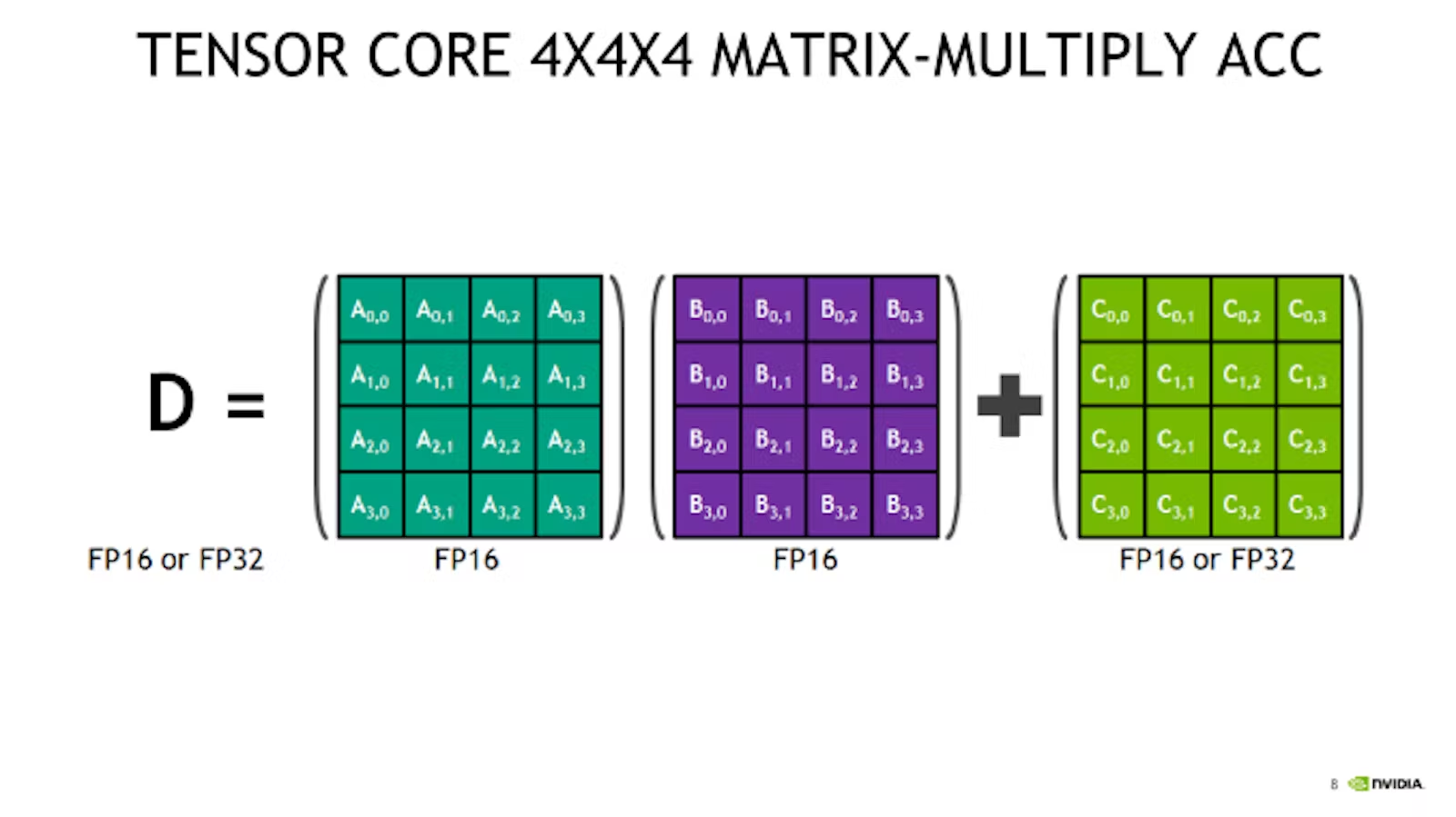
The following figure (source) depicts the fundamental computational pattern executed by a Tensor Core—a fused MMA on small matrix tiles, typically of size 4×4 in early architectures. In this operation, two input matrices (\(A\) and \(B\)), stored in a reduced-precision format such as
float16orbfloat16, are multiplied together. The results of these element-wise multiplications are then summed and accumulated directly into a third matrix (\(C\)), which may be stored in eitherfloat16,bfloat16,float32, or, in newer architectures,float8orfloat4. This fusion of multiplication and accumulation into a single hardware instruction eliminates the need to store intermediate results in memory, drastically reducing memory bandwidth requirements and increasing throughput. Larger GEMM (General Matrix Multiply) operations are implemented by tiling them into many such MMA operations executed in parallel across the GPU’s Tensor Cores.
Definition
- Quantization in the context of deep learning refers to the process of reducing the numerical precision of a model’s parameters (weights) and/or intermediate computations (activations). Typically, models are trained and stored using 32-bit floating-point (
float32) precision. Quantization replaces these high-precision values with lower-precision representations—such as 16-bit floating point (float16), 8-bit integer (int8), 4-bit integer, or binary formats in more extreme scenarios. The primary goals are to reduce model size, improve memory and compute efficiency, and accelerate inference—particularly on hardware that supports low-precision arithmetic. - The primary goal of quantization is to enhance inference speed. In contrast, as will be discussed in the section on Mixed Precision Training, the goal of Automatic Mixed Precision (AMP) is to reduce training time. Quantization is effective, in part, because modern neural networks are typically highly over-parameterized and exhibit robustness to minor numerical perturbations. With appropriate calibration and suitable tools, lower-precision representations can approximate the full-precision model closely enough for practical deployment.
Types of Quantization
-
There are two general categories of quantization:
-
Floating-point quantization: This reduces the bit-width of floating-point values—for example, converting from
float32tofloat16orbfloat16. These formats retain the same general IEEE 754 structure (sign, exponent, mantissa) but use fewer bits, reducing precision and dynamic range. This kind of quantization is primarily used for inference on GPUs and accelerators optimized for low-precision floating-point math (e.g., NVIDIA Tensor Cores). -
Integer quantization: This maps floating-point values to fixed-point integer representations (e.g.,
int8oruint8). This type requires an additional transformation using scale and zero-point to linearly approximate real values using integers, enabling integer-only arithmetic during inference on CPUs and certain edge devices.
-
Integer Quantization
-
Integer quantization is typically implemented as a learned linear transformation (i.e., linear mapping) defined by two parameters: scale and zero-point.
-
The scale is a floating-point multiplier that determines the resolution or step size between adjacent quantized integer values.
-
The zero-point is an integer offset that aligns a real-valued zero to the corresponding integer value in the quantized (i.e., target) range. This allows for asymmetric distributions, where zero is not necessarily centered.
- The forward quantization formula (
floattoint) is:
q = round(x / scale) + zero_point- The reverse dequantization formula (
inttofloat) is:
x = scale * (q - zero_point) - The forward quantization formula (
-
As an example:
- Suppose we want to quantize floating-point values in the range \([-1.0, 1.0]\) to 8-bit unsigned integers (
uint8, range 0–255). The mapping would look like:
scale = (max - min) / (quant_max - quant_min) = (1.0 - (-1.0)) / (255 - 0) ≈ 0.00784 zero_point = round(0 - min / scale) = round(0 - (-1.0 / 0.00784)) = 128- This means that the floating-point value 0.0 maps to 128, 1.0 maps to 255, and -1.0 maps to 0. Intermediate values are linearly interpolated. This transformation enables low-bit integer operations that approximate floating-point behavior.
- Suppose we want to quantize floating-point values in the range \([-1.0, 1.0]\) to 8-bit unsigned integers (
-
Non-Linear Integer Quantization Methods
-
While linear quantization using scale and zero‑point is the most common, non‑linear quantization methods are also employed in integer quantization to better match real-world data distributions. These methods typically apply to integer quantization, as they redefine how integer values map to real numbers:
-
Logarithmic quantization uses exponentially spaced quantization levels—e.g. powers of two—providing better representation across a wide dynamic range. This method is non‑linear and particularly used for integer-only inference pipelines. It is not relevant for floating‑point quantization, which already uses a non‑uniform exponent-based scale inherently built into its representation.
-
K-means or cluster-based quantization groups floating-point values into clusters, mapping each to its centroid—another non-linear approach for integer quantization or weight sharing schemes.
-
Learned transformations, such as LSQ (Learned Step Size Quantization) and its non-uniform variant nuLSQ, optimize quantization step sizes or level spacing via backpropagation. These methods are applied to integer quantization of weights and activations (e.g., 2‑, 3‑, or 4‑bit integer quantization) and involve non-linear quantizer parameterization.
-
In summary, non-linear quantization techniques are relevant for integer quantization workflows, where they redefine integer mapping to better match value distributions. Floating‑point quantization (e.g., float32 \(\rightarrow\) float16/bfloat16), while structurally non-linear due to its exponent/mantissa hierarchy, does not employ these learned or clustering-based non-linear integer mapping schemes.
-
Floating-Point Quantization
- Floating-point quantization is implemented by truncating or rounding the mantissa and exponent fields in IEEE754 representation—e.g. conversion from
float32tofloat16orbfloat16—preserving the format structure but reducing bit-width. This form of quantization (i.e., bit‑width reduction) is non-linear in effect because the quantization steps vary by exponent range: numbers near zero have finer granularity than large values due to the floating-point exponent scaling. - This approach aligns with a well-known model in signal quantization theory often referred to as the compressor–quantizer–expander model. In this framework, the exponential scaling of floating-point numbers acts as a compressor that non-linearly maps real values into a domain where uniform quantization (truncation of mantissa bits) is applied. The quantizer then discretizes the mantissa (hidden quantizer), and the expander step reconstructs the approximate value from the compressed representation. This structure enables efficient representation of a wide dynamic range with relatively coarse quantization, especially benefiting smaller values close to zero.
- Common APIs include casting methods like
model.half()in PyTorch and PyTorch’s support forfloat16static quantization configs (e.g.float16_static_qconfig). Floating-point quantization halves memory footprint with minimal accuracy loss on GPU inference platforms.
Dequantization Considerations
- Dequantization is not always needed during inference, and its necessity depends on the type of quantization and the underlying hardware. In integer-only quantization pipelines—commonly used for inference on mobile CPUs or edge devices—computations are performed entirely in the integer domain (e.g.,
int8oruint8), and dequantization is typically only applied at the final stage, such as for logits or output activations. This avoids floating-point operations altogether during inference.- However, in hybrid quantization workflows, where some layers are quantized (e.g., to
int8) and others remain in higher precision (float32orfloat16), intermediate dequantization is required at the layer boundaries to enable compatibility between quantized and non-quantized components. This is common in models that cannot fully tolerate quantization across all layers due to accuracy degradation or unsupported ops. - In contrast, when quantizing to lower-precision floating-point formats like
float16, dequantization is not needed at all, because these formats are still natively supported by GPU hardware. For example, NVIDIA Tensor Cores are optimized forfloat16(andbfloat16) matrix operations, so models usingfloat16quantization can be executed directly end-to-end without converting back tofloat32. All computations remain in low-precision floating-point format, maintaining performance while avoiding the complexity of dequantization logic entirely.
- However, in hybrid quantization workflows, where some layers are quantized (e.g., to
Quantization Workflows
-
There are three main workflows/approaches to apply quantization:
-
Dynamic / Runtime Quantization: This method quantizes model weights statically (e.g. to
int8orfloat16), while activations remain in full precision until runtime, where they are quantized dynamically at each inference step right before computation. It requires no calibration dataset and no fine‑tuning, making it the easiest quantization method provided by PyTorch. It is particularly effective for models dominated by weight‑heavy layers such astorch.nn.Linear, recurrent layers (nn.LSTM,nn.GRU), and transformers. In PyTorch, this is implemented via the functionquantize_dynamic, for example:import torch quantized_model = torch.ao.quantization.quantize_dynamic( model_float32, {torch.nn.Linear, torch.nn.LSTM}, dtype=torch.qint8 )- With this approach, the quantized model is memory‑efficient and can accelerate inference for NLP architectures, often with negligible accuracy loss compared to PTQ—though with lower benefit on convolution‑heavy vision models.
- Look up the Dynamic / Runtime Quantization section for a detailed discourse on this topic.
-
Post-Training Quantization (PTQ): Converts a fully trained high-precision model to a lower-precision format without retraining. PTQ typically uses a calibration dataset to compute appropriate
scaleandzero-pointvalues using strategies like min-max range or percentile clipping. It is simple to use and well-supported in frameworks such as TensorFlow Lite and PyTorch, but may incur accuracy loss—particularly for sensitive or activation-heavy layers.- From the TensorFlow post-training quantization documentation:
We generally recommend 16-bit floats for GPU acceleration and 8-bit integer for CPU execution.
- This reflects hardware preferences:
float16enables faster matrix multiplications on GPU accelerators like Tensor Cores, whileint8is more efficient on CPU architectures with dedicated integer units such as integer SIMD extensions (e.g., AVX, NEON, VNNI). - Look up the Post-Training Quantization section for a detailed discourse on this topic.
-
Quantization-Aware Training (QAT): In QAT, quantization effects—specifically the non-linearity introduced by rounding and clipping—are simulated during training, allowing the model to adapt. The model behaves as though it operates in lower precision during the forward pass, using the quantization formula above with fake quantization modules (e.g.,
FakeQuantizein PyTorch ortf.quantization.fake_quant_with_min_max_varsin TensorFlow). These modules apply quantization and dequantization logic using scale and zero-point. However, backpropagation remains in full precision. In other words, gradients and parameter updates are still computed using fullfloat32precision. This allows the model to adapt to quantization-induced noise, often resulting in better accuracy retention compared to PTQ. QAT is especially useful when targeting very low-bit formats (such as 4-bit or lower) or when quantizing sensitive components like attention layers in transformers or deploying models in high-accuracy applications.- Look up the Quantization‑aware Training (QAT) section for a detailed discourse on this topic.
-
Benefits and Limitations
- Quantization can lead to significant reductions in efficiency, both in terms of memory footprint and computational load. For example, converting
float32weights toint8reduces storage requirements by 75%, and on supported hardware, can improve inference speed by 2× to 4×. These benefits are amplified on edge devices with limited memory, power, and compute such as mobile phones, IoT sensors, embedded processors, and accelerators that support low-precision execution.
While quantization offers compelling advantages, it can also suffer from practical limitations. Quantization might not work uniformly well across all architectures or layers since some operators (powering these layers and architectures) might not be supported in quantized form on all hardware targets. Put simply, some hardware can lack native support for certain quantized operators, since they typically have to be implemented individually. Operators like group convolutions, custom layers, normalization approaches (say LayerNorm), etc. may fall back to
float32or require custom low-level kernels, potentially limiting compatibility or efficiency on target platforms. Lastly, layers with small value ranges, heavy outliers, or complex nonlinear interactions may require higher precision (e.g.,float16orfloat32) to avoid accuracy degradation.
Mitigation Strategies
-
Selective strategies like per-channel, per-group, per-layer, per-tensor, and mixed-precision quantization are commonly used to mitigate limitations such as accuracy loss, hardware incompatibilities, and uneven value distributions across layers.
-
Per-channel quantization (also referred to as channel-wise quantization): This approach assigns separate scale and zero-point values to each output channel of a weight tensor. It is particularly effective in convolutional and linear layers where each output channel (or filter) may have significantly different weight distributions. By capturing channel-wise variations in magnitude, it provides better quantization accuracy, especially in vision models like ResNet, MobileNet, and EfficientNet, as well as transformer-based architectures such as BERT and GPT. PyTorch implements this using the
torch.per_channel_affinequantization scheme. -
Per-group quantization (also referred to as group-wise quantization): A compromise between per-tensor and per-channel quantization. Channels are divided into groups, with each group sharing quantization parameters. This reduces the overhead of storing separate scale/zero-point values for every channel, while still preserving more distributional information than per-tensor quantization. It is particularly useful in resource-constrained deployment scenarios where memory and compute costs must be balanced against accuracy. Though not always exposed via high-level APIs in frameworks like PyTorch, this strategy is supported in certain hardware accelerators and vendor-specific toolchains (e.g., Qualcomm, MediaTek, Xilinx).
-
Per-layer quantization (also referred to as layer-wise quantization): This applies the same quantization parameters (scale and zero-point) across an entire layer’s output or weight tensor. For example, all outputs of a linear layer or all weights of a convolution kernel are quantized using a single shared set of parameters. This method is computationally efficient and requires minimal additional metadata, making it widely used in low-resource settings or for fast prototyping. However, it often leads to higher quantization error in layers with highly varied internal distributions.
-
Per-tensor quantization (also referred to as tensor-wise quantization): A special case of per-layer quantization where quantization is applied uniformly across an entire tensor (typically weight or activation). A single scale and zero-point are calculated for the full tensor, regardless of dimensionality or channel boundaries. This is the simplest and most lightweight quantization method, requiring minimal bookkeeping and fast execution. While effective for layers with narrow and uniform value ranges, it can result in significant information loss when used on tensors with wide dynamic range or uneven channel statistics. This method is often the default in early-stage quantization workflows or on hardware that does not support fine-grained schemes.
-
Mixed-precision quantization: Instead of applying uniform quantization across all model layers, mixed-precision quantization selectively retains higher-precision (e.g.,
float32orfloat16) computation in layers that are sensitive to quantization noise—such as attention heads, layer normalization, or output classifiers. Other layers, particularly early convolution blocks or MLPs, can be safely quantized toint8or lower. This approach enables developers to achieve a favorable trade-off between accuracy and efficiency. Mixed-precision is supported by most modern inference engines including TensorRT, TVM, XNNPACK, and PyTorch FX Graph Mode Quantization.
Weights vs. Activation Quantization
-
Why they’re not the same: Weights and activations have fundamentally different roles and constraints during quantization.
-
Weights are static once training completes. Since they do not vary across inputs, they may be quantized offline using fixed calibration data or analytically via heuristics such as min‑max scaling or percentile statistics. This allows more aggressive optimization techniques such as per‑channel quantization or non‑uniform quantization, and values may be precomputed and stored in compact low‑precision formats like
int8,int4, or binary. -
Activations, by contrast, are dynamic and input‑dependent. Their value ranges vary based on data processed during inference. Therefore, activation quantization must accommodate runtime variability. Two common modes exist:
-
Static Activation Quantization: Calibration datasets estimate typical activation ranges (min/max or histogram‑based) per layer. These statistics are then used to assign fixed scale/zero‑point pairs for quantized representation, using observers such as
MinMaxObserveror histogram‑based observers. -
Dynamic Activation Quantization: During inference, scale and zero‑point values are computed on‑the‑fly from input‑dependent statistics (e.g. dynamic min/max per batch). This avoids calibration datasets but may add latency due to runtime computation.
-
-
-
Handling outliers: Outliers in activation or weight distributions can drastically degrade quantization quality by skewing range and reducing effective precision. Several mitigation strategies include:
-
Percentile‑based Clipping: Rather than using absolute min/max, activations may be clipped to a percentile‑based range (e.g. 99.9%) to discard extreme outliers. Techniques include KL divergence minimization or MSE‑based clipping, used in frameworks such as PyTorch or TensorFlow Lite.
-
Per‑Channel Quantization: Instead of applying a single scale across a tensor, per‑channel quantization assigns unique scale and zero‑point values per output channel. This adapts to local distribution variations, particularly in convolutional or linear layers. In PyTorch, this is implemented via PerChannelMinMaxObserver or similar observers using
torch.per_channel_affineschemes. Core functions includetorch.quantize_per_channelandtorch.fake_quantize_per_channel_affineto simulate quantization.-
Per‑channel quantization is especially effective in:
- Convolutional neural networks (e.g. ResNet, MobileNet, EfficientNet, YOLO), where filter/channels have distinct distribution ranges.
- Transformer architectures (e.g. multi‑head attention or feed‑forward layers), where weight and activation distributions vary widely across heads or projection layers.
-
-
Learned Scale Factors: Methods like Learned Step Size Quantization (LSQ), introduced in the paper “Learned Step Size Quantization” by Esser et al. (2020), enable scale parameters to be optimized via backpropagation during fine‑tuning. This adaptive scaling is especially beneficial in models with skewed distributions—such as transformer-based language models, where operations like softmax produce skewed outputs.
-
-
Advanced Weight Handling:
-
Per‑Group Quantization: Instead of full per‑channel (i.e. one scale per channel), per‑group quantization assigns one scale per group of channels (e.g. N channels or per row). This balances granularity and memory overhead and is prevalent in formats like ONNX or TensorRT.
-
Activation‑Aware Weight Quantization (AWQ): AWQ techniques tailor weight quantization ranges and groupings using activation patterns observed during calibration. Rather than uniformly quantizing weights, these methods use sensitivity analysis to allocate bit budgets or adjust grouping for performance‑critical weights.
-
Zero‑Point Optimization: For symmetric quantization (typically weight tensors), zero‑point is fixed at zero. For asymmetric quantization—commonly used for activations—the zero‑point shifts the quantized range. Some frameworks (e.g. ONNX, TensorFlow Lite) allow fine‑grained control over zero‑point alignment, which influences both accuracy and hardware compatibility.
-
-
In practice, weight and activation quantization are applied jointly but with distinct parameter sets and calibration workflows. Modern toolkits support fine-grained configuration, including:
- PyTorch’s torch.quantization and torch.ao.quantization modules;
- TensorFlow Model Optimization Toolkit (quantization guide) supporting calibration APIs and quantization-aware training;
- NVIDIA TensorRT, which enables layer-wise quantization, quantization-aware training, and PTQ via its TensorRT SDK documentation and the Torch‑TensorRT Model Optimizer;
- Intel Neural Compressor, an open‑source framework offering post‑training static, dynamic, and quantization‑aware training workflows for PyTorch and TensorFlow (Intel Neural Compressor documentation).
Effective quantization requires balancing statistical rigor, hardware compatibility, and architecture sensitivity. Activations require runtime awareness, while weights benefit from static optimization—and both may leverage learned or adaptive scaling to maintain fidelity in low‑bit regimes.
Quantization with PyTorch
-
Quantization in PyTorch enables the execution of computations and memory accesses with reduced-precision data types, typically
int8, leading to improvements in model efficiency, inference speed, and memory footprint. PyTorch provides comprehensive support for quantization, starting from version 1.3, through an API that integrates seamlessly with the existing eager execution model. -
Quantized Tensor Representation
-
PyTorch introduces special data types for quantized tensors, enabling the representation of weights and activations in reduced precision (typically
int8, and sometimesfloat16). These tensors can be operated on via quantized kernels available undertorch.nn.quantizedandtorch.nn.quantized.dynamic. These quantized operations allow for a 4× reduction in model size and 2-4× improvements in memory bandwidth and inference latency, depending on the hardware and model structure. -
Quantization in PyTorch relies on calibration, which is the process of gathering statistics on representative inputs to determine optimal quantization parameters (such as scale and zero-point). These parameters are used in quantization functions of the form
round(x / scale) + zero_point, enabling a linear mapping between floating point and integer domains.
-
-
Quantization Backends
- PyTorch leverages optimized backend libraries to execute quantized operations efficiently. FBGEMM (Facebook’s GEMM library) is optimized for server environments (x86 CPUs), while QNNPACK is designed for mobile and embedded environments. These are analogous to BLAS/MKL libraries in floating-point computation and are integrated automatically based on the target deployment platform.
-
Numerical Stability and Mixed Precision
- One challenge in quantization is maintaining numerical stability, particularly for operations involving accumulation or exponentiation. To address this, PyTorch supports mixed-precision training and inference using the
torch.cuda.ampmodule. AMP (Automatic Mixed Precision) allows portions of the model to be cast totorch.float16while retainingtorch.float32for operations requiring higher precision, improving performance with minimal loss of accuracy. Although initially introduced for CUDA GPUs, mixed-precision techniques are distinct from quantization but can be complementary in certain scenarios.
- One challenge in quantization is maintaining numerical stability, particularly for operations involving accumulation or exponentiation. To address this, PyTorch supports mixed-precision training and inference using the
-
Quantization Techniques in PyTorch
-
PyTorch provides three primary quantization workflows under the
torch.quantizationnamespace, often referred to collectively as “eager mode quantization”: - Dynamic Quantization:
-
Weights are statically quantized and stored in int8 format, while activations are dynamically quantized at runtime before computation. This method requires minimal code changes and no calibration data. It is most effective for models dominated by linear layers (e.g., LSTM, GRU, Transformer-based models).
-
Example:
torch.quantization.quantize_dynamic(model, {torch.nn.Linear}, dtype=torch.qint8) -
- Post-Training Quantization:
-
Both weights and activations are quantized. This approach requires calibration, where representative input data is passed through the model to collect statistics via observer modules. Operator fusion (e.g., Conv + ReLU) and per-channel quantization are supported to improve performance and accuracy.
-
Example sequence:
model.qconfig = torch.quantization.get_default_qconfig('fbgemm') torch.quantization.prepare(model, inplace=True) # Run calibration with representative data torch.quantization.convert(model, inplace=True) -
- Quantization-Aware Training (QAT):
-
This technique inserts fake-quantization modules during training, simulating quantization effects in both forward and backward passes. It typically yields the highest post-quantization accuracy, especially in cases where model accuracy is sensitive to quantization noise.
-
Example sequence:
model.qconfig = torch.quantization.get_default_qat_qconfig('fbgemm') torch.quantization.prepare_qat(model, inplace=True) # Train model torch.quantization.convert(model.eval(), inplace=True) -
-
-
Operator and Layer Coverage
- Quantization support varies by method. Dynamic quantization supports layers like Linear and RNNs, while static and QAT methods support a broader set including Conv, ReLU, BatchNorm (via fusion), and more. FX Graph Mode Quantization (a newer, graph-level approach not covered here) further expands operator support and streamlines workflows.
-
For additional guidance and end-to-end examples, refer to the official PyTorch blog: Introduction to Quantization on PyTorch.
Dynamic / Runtime Quantization
-
Dynamic quantization is one of the most simple quantization techniques in PyTorch, particularly suitable for models where most computation occurs in linear layers—such as transformer models (e.g. BERT) or recurrent networks (e.g. LSTM)—because these operations are dominated by matrix multiplications, which benefit significantly from
int8acceleration without requiring quantized convolutions. -
In dynamic quantization, model weights are converted from 32-bit floating point (
float32) to a lower precision format such asint8and are permanently stored in this quantized form. Activations, however, remain infloat32format until runtime. At inference time, these activations are dynamically quantized toint8immediately before the corresponding computation (i.e., matrix multiplication or linear operation) is executed. After the operation, the result is stored back infloat32. This hybrid approach enables significant performance gains—such as reduced latency and memory usage—while maintaining reasonable model accuracy.
The aim of dynamic quantization is thus to save compute through faster arithmetic, rather than primarily to reduce storage needs.
-
Unlike static quantization or quantization-aware training (QAT), dynamic quantization requires no calibration dataset or retraining. This makes it ideal when representative data is unavailable or ease of deployment is paramount.
-
Quantization parameters (scale and zero-point) for activations are determined dynamically at each invocation based on the input data range, while weights use fixed scale and zero-point values computed ahead of time. As such, since only the model weights are quantized ahead of time, while activations remain in
float32and are quantized dynamically at runtime based on input data, dynamic quantization is often referred to as a data-free or weight-only quantization method during preparation. -
PyTorch provides the API
torch.ao.quantization.quantize_dynamic(...)for applying dynamic quantization:- A model (
torch.nn.Module) - A specification of target layer types or names (commonly
{nn.Linear, nn.LSTM}) - A target dtype (e.g.,
torch.qint8).
- A model (
-
Only supported layer types are quantized—primarily
nn.Linearand RNN variants; convolutional layers (e.g.,nn.Conv2d) are not supported by dynamic quantization. -
This approach is particularly effective for transformer and RNN models, where inference throughput is limited by memory-bound weight matrices. For example, quantizing BERT with dynamic quantization often yields up to 4× reduction in model size and measurable speedups in CPU inference latency.
Dynamic Quantization vs. Post-Training Quantization
- Unlike Post-Training Quantization, dynamic quantization does not use minmax observers or any calibration mechanism. Activation ranges are computed dynamically at runtime based on actual input data, so no observers are required during model preparation.
Example Workflow
- Below is an example illustrating a typical dynamic quantization workflow:
import torch
from torch import nn
from torch.ao.quantization import quantize_dynamic

# Assume `model` is a pretrained floating‑point nn.Module, in eval mode
model.eval()

# Apply dynamic quantization to Linear and LSTM layers
quantized_model = quantize_dynamic(
    model,
    {nn.Linear, nn.LSTM},
    dtype=torch.qint8
)

# Run inference: activations will be quantized at runtime
input_data = torch.randn(batch_size, seq_length, feature_dim)
output = quantized_model(input_data)
Workflow Explanation
model.eval()ensures deterministic behavior during quantization.quantize_dynamic(...)replaces supported layers with their dynamic quantized implementations.- Activations remain in
float32until needed. - At runtime, activations are quantized to
int8on-the-fly, and computations are performed withint8weights and mixed precision accumulators. - After the operation, results return to
float32.
Typical Benefits
- Model size reduced by ~75%, thanks to
int8weights. - Latency improvements, especially on CPU-bound operations.
- No calibration or fine-tuning required.
Notes & Trade‑offs
- Dynamic quantization does not support convolution or custom layers unless manually wrapped.
- Dynamic quantization handles input distributions that vary widely more gracefully than static quantization, which uses fixed calibration ranges.
- For CNN models or workloads where activations must also be quantized ahead of time, static quantization or QAT may yield better performance and accuracy.
Further Reading
- A comprehensive end-to-end tutorial for dynamic quantization on BERT is available here.
- For a more general example and advanced usage guide, see the dynamic quantization tutorial.
- The full API documentation for
torch.quantization.quantize_dynamicis available here.
Post-Training Quantization
-
Post-Training Quantization (PTQ) is a technique in PyTorch that enables the conversion of a model’s weights and activations from floating-point (typically
float32) to 8-bit integers (int8), significantly improving inference efficiency in terms of speed and memory usage. This method is particularly well-suited for deployment scenarios on both server and edge devices, where latency and resource constraints are critical. -
To facilitate this process, PyTorch inserts special modules known as observers into the model. These modules capture the activation ranges at various points in the network. Once sufficient data has been passed through the model during calibration, the observers record min-max values or histograms (depending on the observer type), which are then used during quantization.
-
A key benefit of static quantization is that it allows quantized values to be passed between operations directly, eliminating the need for costly float-to-int and int-to-float conversions at each layer. This optimization significantly reduces runtime overhead and enables end-to-end execution in
int8. -
PyTorch also supports several advanced features to further improve the effectiveness of static quantization:
-
Observers:
- Observer modules are used to collect statistics on activations and weights during calibration. These can be customized to suit different data distributions or quantization strategies. PyTorch provides default observers like
MinMaxObserverandHistogramObserver, and users can register them via the model’sqconfig. - Observers are inserted using
torch.quantization.prepare.
- Observer modules are used to collect statistics on activations and weights during calibration. These can be customized to suit different data distributions or quantization strategies. PyTorch provides default observers like
-
Operator Fusion:
- PyTorch supports the fusion of multiple operations (e.g., convolution + batch normalization + ReLU) into a single fused operator. This reduces memory access overhead and improves both runtime performance and numerical stability.
- Modules can be fused using
torch.quantization.fuse_modules.
-
Per-Channel Weight Quantization:
- Instead of applying the same quantization parameters across all weights in a layer, per-channel quantization independently quantizes each output channel (particularly in convolution or linear layers). This approach improves accuracy while maintaining the performance benefits of quantization.
- Final conversion to the quantized model is done using
torch.quantization.convert.
-
Post-Training Quantization vs. Dynamic Quantization
- Unlike dynamic quantization, which quantizes activations on-the-fly during inference, static quantization requires an additional calibration step. This calibration involves running representative data through the model to collect statistics on the distribution of activations. These statistics guide the quantization process by determining appropriate scaling factors and zero points for each tensor.
- Put simply, in PTQ, while weights are quantized ahead of time, activations are quantized using calibration data collected via observers, enabling fully quantized inference across all layers.
Example Workflow
- Below is an example illustrating a typical PTQ workflow:
import torch
import torch.quantization

# Step 1: Define or load the model
model = ...  # assume a pre-trained model is loaded

# Step 2: Set the quantization configuration
# Choose backend depending on target device
model.qconfig = torch.quantization.get_default_qconfig('qnnpack')  # for ARM/mobile
# model.qconfig = torch.quantization.get_default_qconfig('fbgemm')  # for x86/server

# Step 3: Fuse modules (e.g., Conv + BN + ReLU)
model_fused = torch.quantization.fuse_modules(model, [['conv', 'bn', 'relu']])

# Step 4: Insert observer modules
model_prepared = torch.quantization.prepare(model_fused)

# Step 5: Calibrate the model with representative data
# For example, run a few batches of real or synthetic inputs
model_prepared(example_batch)

# Step 6: Convert to a quantized model
model_quantized = torch.quantization.convert(model_prepared)
- This static quantization pipeline can yield 2× to 4× speedups in inference latency and a 4× reduction in model size, with minimal degradation in accuracy when calibrated effectively.
Workflow Explanation
-
After the example workflow, here is a breakdown of each step and its purpose:
- Model Preparation: The model must be in eval mode (
model.eval()) so that observers and quantization stubs function deterministically. Depending on the backend,model.qconfig = torch.ao.quantization.get_default_qconfig('x86')or'qnnpack'sets the appropriate quantization configuration. - Operator Fusion: Use
torch.quantization.fuse_modulesto merge modules like Conv‑BatchNorm‑ReLU into a single fused operator. This improves numerical stability and reduces redundant quant‑dequant steps. - Observer Insertion: Invoke
torch.quantization.prepareto automatically insert observer modules (e.g.,MinMaxObserver). These record activation statistics during the calibration phase. - Calibration: Run representative real-world input data through the prepared model to collect min/max or histogram statistics via observers. Approximately 100‑200 mini‑batches often suffice for good calibration.
- Conversion to Quantized Model: Use
torch.quantization.convertto replace observed layers with quantized counterparts, applying pre-determined scales and zero points. The resulting model executes end‑to‑end inint8arithmetic.
- Model Preparation: The model must be in eval mode (
Typical Benefits
- Model size is typically reduced by ≈4× (since
int8requires only 1 byte per parameter instead of 4) and memory bandwidth requirements drop significantly. - Inference latency improves—often 2× to 4× faster than float32—by eliminating repeated float‑int conversions and enabling optimized integer kernels on CPU and mobile.
- Enables uniform quantized execution across the network, which improves cache locality and enables hardware acceleration on supported platforms.
Notes & Trade‑offs
- Requires a representative calibration dataset. If the input distribution drifts significantly, fixed quantization ranges may degrade accuracy over time.
- Slight accuracy loss compared to floating‑point baseline—although typically small (~1‑2%)—especially on highly non-linear or sensitive models. For critical accuracy use‑cases, Quantization Aware Training may be more suitable.
- Not all operators are supported for eager/static quantization. While convolution, linear, and RNN layers are supported, custom or unsupported layers may need manual handling or fallbacks. Per-channel quantization support is available, but requires proper qconfig settings.
- The quantization workflow in PyTorch uses either Eager Mode or FX Graph Mode. FX mode can automate fusion and support functional operators, but may require model refactoring. Eager Mode offers more manual control but with limited operator coverage.
Quantization‑aware Training (QAT)
-
QAT is the most accurate among PyTorch’s three quantization techniques for static quantization. With QAT, all weights and activations are subject to “fake quantization” during both forward and backward passes: values are rounded to simulate
int8quantization, while computations remain in floating‑point. Consequently, weight updates occur with full awareness that the model will eventually operate inint8. As a result, models trained with QAT generally achieve higher post‑quantization accuracy than those produced by post‑training quantization or dynamic quantization. -
The principle is straightforward: the training process is informed about the ultimate quantized inference format. During training, activations and weights are rounded appropriately, so gradient flow reflects the quantization effects. However, the backpropagation itself—the gradient descent—is executed using full‑precision arithmetic.
-
After QAT training and conversion, the final model stores both weights and activations in the
int8quantized format, making it suitable for efficient inference on quantization-compatible hardware. -
To implement QAT in PyTorch’s eager‑mode workflow, one typically follows these steps:
- Fuse suitable modules (e.g. Conv+ReLU, Conv+BatchNorm) via
torch.quantization.fuse_modules. - Insert
QuantStubandDeQuantStubmodules to manage quantization boundaries. - Assign
.qconfigto modules—e.g. viatorch.quantization.get_default_qat_qconfig('fbgemm')or'qnnpack'. - Prepare the model using
torch.ao.quantization.prepare_qat()ortorch.quantization.prepare_qat(). - Train or fine‑tune the model in training mode.
- After training, apply
torch.ao.quantization.convert()ortorch.quantization.convert()to produce the fully quantizedint8model.
- Fuse suitable modules (e.g. Conv+ReLU, Conv+BatchNorm) via
-
A code snippet in PyTorch invoking QAT:
qat_model.qconfig = torch.quantization.get_default_qat_qconfig('fbgemm')
torch.quantization.prepare_qat(qat_model, inplace=True)
# train or fine‑tune qat_model ...
quantized_model = torch.quantization.convert(qat_model.eval(), inplace=False)
- The fake quantization modules, which simulate the effects of quantization during both forward and backward passes, internally use observers (e.g.,
MinMaxObserverorHistogramObserver) to track activation and weight ranges during training. These fake quantization modules, which are inserted during training, are typically replaced with real quantized operators in the converted model.
Quantization‑aware Training vs. Post-Training Quantization vs. Dynamic Quantization
- Note that unlike dynamic quantization (which only quantizes weights statically and activations on-the-fly during inference), QAT simulates quantization for both weights and activations during training. This allows the model to learn parameters that are robust to quantization-induced errors introduced at inference time. Put simply, it allows the parameters to adapt to quantization noise during inference and typically results in significantly better accuracy, especially for models with activation-sensitive layers such as convolutional networks.
- Furthermore, unlike post-training quantization, QAT does not require a separate calibration phase after training. Instead, it uses the observer modules during training itself to learn and track the necessary quantization parameters, effectively integrating calibration into the training loop.
Example Workflow
- This sub‑section illustrates a complete workflow for applying static QAT to a convolutional neural network (e.g. ResNet18):
import torch
import torch.nn as nn
import torch.quantization
from torch.quantization import QuantStub, DeQuantStub

class MyModel(nn.Module):
    def __init__(self):
        super().__init__()
        self.quant = QuantStub()
        self.conv = nn.Conv2d(3, 16, kernel_size=3, stride=1, padding=1)
        self.bn = nn.BatchNorm2d(16)
        self.relu = nn.ReLU()
        self.fc = nn.Linear(16*32*32, 10)
        self.dequant = DeQuantStub()

    def forward(self, x):
        x = self.quant(x)
        x = self.relu(self.bn(self.conv(x)))
        x = x.flatten(1)
        x = self.fc(x)
        x = self.dequant(x)
        return x

# 1. Load pre‑trained or float‑trained model
model = MyModel()
model.eval()

# 2. Fuse conv, bn, relu
torch.quantization.fuse_modules(model, [['conv','bn','relu']], inplace=True)

# 3. Attach QAT config
model.qconfig = torch.quantization.get_default_qat_qconfig('fbgemm')

# 4. Prepare QAT
torch.quantization.prepare_qat(model, inplace=True)

# 5. Fine‑tune QAT model
model.train()
# run training loop for several epochs ...

# 6. Convert to quantized model
quantized_model = torch.quantization.convert(model.eval(), inplace=False)

# 7. Evaluate quantized_model for accuracy and inference performance
Workflow Explanation
- This workflow enforces quantization effects during training by simulating rounding and clamping via fake quantization modules.
QuantStubandDeQuantStubdemarcate where data transitions between float and quantized domains.qconfigcontrols observer placement and quantization schemes (e.g. symmetric vs affine, per‑tensor vs per‑channel). - Fake quantization is active during training, guiding the network to adapt to the constraints of int8 inference arithmetic. Only after fine‑tuning does
convert()replace fake quant modules with actual quantized operators for efficientint8inference execution.
Typical Benefits
- Higher quantized accuracy than post‑training static or dynamic quantization, often reducing performance degradation to minimal levels.
- Improved robustness to quantization noise, particularly important for convolutional networks and vision models.
- Retains compression benefits: reduced model size (≈25% of float model) and faster inference on hardware optimized for
int8.
Notes & Trade‑offs
- QAT requires additional training or fine‑tuning, increasing overall development time.
- Careful scheduling is needed: a small learning rate is recommended to avoid instability introduced by straight‑through estimator (STE) approximations.
- Model preparation steps such as layer fusion and correct placement of quant stubs are critical. Missing fusions can degrade accuracy.
- Not all operators or model architectures are fully quantization‑aware; some require manual adaptation.
- The quantized model behavior may differ subtly from the fake‑quant version: as reported, the output of a real quantized model may diverge slightly from fake‑quant during testing on toy models.
Comparative Analysis
- Here is a detailed comparative analysis of Dynamic Quantization, PTQ, and QAT:
| Aspect | Dynamic / Runtime Quantization | Post-Training Quantization (PTQ) | Quantization-Aware Training (QAT) |
|---|---|---|---|
| Primary Use Case | Fast, easy quantization of models with primarily linear operations (e.g. LSTM, BERT) | Quantization of convolutional or more complex models with moderate accuracy tradeoff | High-accuracy quantization for models sensitive to quantization (e.g. CNNs, object detectors) |
| Requires Retraining? | No | No | Yes |
| Requires Calibration Data? | No | Yes (to collect activation statistics) | No separate calibration; statistics are collected during training |
| When Activations Are Quantized | At runtime (dynamically before each operation) | Statically using observer statistics from calibration | During training using fake quantization modules |
| Quantization of Weights | Done ahead of time (static) | Done ahead of time (static) | Simulated during training, finalized during conversion |
| Quantization of Activations | Dynamically quantized at inference time | Statically quantized using calibration ranges | Simulated via fake quantization during training |
| Typical Accuracy | Moderate loss (acceptable for linear-dominant models) | Slight to moderate loss | Minimal loss; best accuracy among all methods |
| Complexity of Setup | Very low | Moderate | High |
| Computation Format During Training | Full float32 | Full float32 | Simulated int8 via fake quantization in float32 |
| Final Inference Format | int8 weights, float32 activations outside ops | int8 weights and activations | int8 weights and activations |
| Deployment Readiness | Easy and quick to apply, suitable for rapid deployment | Requires calibration workflow | Requires full training pipeline |
| Main Benefit | Faster inference via int8 compute; no data or retraining needed | Reduced latency and memory with moderate setup | Maximum accuracy with full int8 inference |
| Target Operators | Mostly linear layers (e.g. nn.Linear, nn.LSTM) |
Broad operator support with fused modules (e.g. Conv+ReLU) |
Full model coverage with operator fusion and training |
| Memory Footprint Reduction | Partial (activations still float32) | Full (weights and activations in int8) | Full (weights and activations in int8) |
| Primary Optimization Goal | Compute efficiency (faster matmuls), leading to latency savings | Latency and memory savings | Accuracy preservation under quantization |
| Example Usage | torch.quantization.quantize_dynamic |
prepare, calibrate, convert |
prepare_qat, train, convert |
Compute vs. Memory Bottlenecks
-
Deep learning performance is typically constrained by one of two primary bottlenecks: compute (arithmetic throughput) or memory (bandwidth and capacity). The balance between them depends on the hardware architecture, the model’s structure, and the numerical precision used.
-
Compute-Bound Workloads:
-
A workload is compute-bound when the GPU/CPU spends most of its time performing arithmetic operations rather than waiting for data from memory. This is common in:
- Large matrix multiplications with high arithmetic intensity (high FLOPs-to-bytes ratio).
- Dense layers and convolution layers with large channel counts and large kernel sizes.
- Transformer attention mechanisms with large batch sizes or long sequence lengths.
-
In compute-bound scenarios, lowering the precision of operands (e.g.,
float32\(\rightarrow\)float16orint8) allows hardware to execute more operations per clock cycle. For example:- NVIDIA Tensor Cores can deliver up to 2×–4× the throughput for
float16orbfloat16GEMMs compared tofloat32. - Integer accelerators (e.g.,
int8SIMD or systolic arrays) can achieve even higher gains, especially on CPUs or edge NPUs.
- NVIDIA Tensor Cores can deliver up to 2×–4× the throughput for
-
By reducing the number of bits per operand, quantization directly increases the number of multiply-accumulate operations that can be executed in parallel within the same silicon area and clock period.
-
-
Memory-Bound Workloads:
-
A workload is memory-bound when the processor spends more time fetching/storing data than performing arithmetic. This is common when:
- The layer has small arithmetic intensity, such as pointwise operations or small matrix-vector products.
- Batch sizes are small, reducing the amount of computation per data load.
- Model parameters or activations exceed on-chip cache capacity, forcing frequent DRAM access.
-
Memory-bound operations are limited by memory bandwidth and latency rather than raw compute throughput. Here, quantization helps by:
- Reducing memory footprint: Lower precision reduces the size of weights and activations (e.g.,
float32\(\rightarrow\)int8cuts memory use by 75%). - Improving cache locality: More parameters fit in L1/L2 cache or shared memory, reducing expensive DRAM fetches.
- Increasing effective bandwidth: Smaller data transfers mean more elements can be moved per memory transaction.
- Reducing memory footprint: Lower precision reduces the size of weights and activations (e.g.,
-
On many edge devices, memory-bound layers see the largest relative speedups from quantization because external DRAM bandwidth is a critical bottleneck.
-
-
Mixed Bottleneck Scenarios:
-
Many real-world models contain both compute-bound and memory-bound regions:
- Early convolution layers in vision models often run close to peak compute throughput, benefiting most from Tensor Core–accelerated low-precision compute.
- Later layers with smaller spatial dimensions but large channel counts may become memory-bound, benefiting more from reduced memory bandwidth pressure than raw FLOP gains.
- Transformer feed-forward layers can be compute-bound, while embedding lookups or normalization layers can be memory-bound.
-
In such cases, mixed-precision quantization can optimize each region separately—keeping sensitive, low-intensity operations in higher precision while aggressively quantizing compute-heavy layers.
-
-
Where Quantization Delivers the Most Impact:
-
Quantization is most impactful when:
- The model runs on hardware with specialized low-precision units (Tensor Cores,
int8MAC units,float8engines). - Memory bandwidth is a limiting factor (common in mobile SoCs, edge AI chips, or when serving many inference requests in parallel).
- Model size exceeds cache capacity, leading to frequent DRAM access.
- Deployment constraints demand both latency and memory footprint reductions (e.g., real-time inference on embedded systems).
- The model runs on hardware with specialized low-precision units (Tensor Cores,
-
-
In summary, quantization addresses compute bottlenecks by enabling more operations per cycle and memory bottlenecks by reducing data transfer volume and improving cache utilization. Understanding which bottleneck dominates for a given layer or model is key to selecting the right quantization strategy.
Modern Quantization Techniques
GPTQ: Quantization with Second-Order Error Compensation
-
Introduced in GPTQ: Accurate Post-Training Quantization for Generative Pre-trained Transformers by Frantar et al. (2023), GPTQ is a high-accuracy post-training quantization (PTQ) method tailored for large-scale transformers. Unlike round-to-nearest schemes, GPTQ minimizes the quantization error using approximate second-order information derived from the Hessian of the loss. It quantizes weights in a layer-wise fashion while updating unquantized weights to compensate for introduced error, achieving efficient
int3/4quantization of models as large as OPT-175B or BLOOM-176B without finetuning. Practical implementations are available through AutoGPTQ and LLM.int4. -
GPTQ significantly outperforms simple rounding methods by preserving perplexity under low-bit quantization. Notably, it is one of the few techniques that scales to 100B+ parameter models using modest compute (e.g., a single A100 GPU). While it focuses on weight-only quantization, activation quantization can be layered on top via orthogonal techniques such as SmoothQuant.
Process
-
Layer-Wise Quantization Objective
-
For a linear layer with weight matrix \(W\) and input activations \(X\), GPTQ minimizes the reconstruction error after quantization:
\[\min_{\hat{W}} \| WX - \hat{W}X \|_2^2\] -
Quantization is performed column-by-column (i.e., per weight vector), and compensation is applied to unquantized weights to preserve the overall output fidelity.
-
-
Approximate Second-Order Weight Selection (OBQ Foundation)
-
GPTQ builds on the Optimal Brain Quantization (OBQ) framework, which selects the next weight \(w_q\) to quantize by minimizing its induced error, scaled by its Hessian diagonal element:
\[w_q = \arg\min \frac{(\text{quant}(w_q) - w_q)^2}{[H^{-1}]_{qq}}, \quad \delta = -\frac{w_q - \text{quant}(w_q)}{[H^{-1}]_{qq}} (H^{-1})_{:,q}\] -
The inverse Hessian \(H^{-1} = (2X X^\top + \lambda I)^{-1}\) captures sensitivity of the layer outputs to changes in weights. This allows for compensation of quantization-induced error by adjusting the remaining unquantized weights.
-
-
Blockwise Column Quantization with Shared Hessian
-
GPTQ introduces the insight that, in large layers, quantizing all rows in a fixed column order yields nearly the same accuracy as a greedy per-weight order.
-
This allows sharing the Hessian across rows and amortizing its computation—resulting in a complexity reduction from \(O(d_{\text{row}} \cdot d_{\text{col}}^3)\) to \(O(\max(d_{\text{row}} \cdot d_{\text{col}}^2, d_{\text{col}}^3))\).
-
The following figure (source) illustrates the GPTQ quantization procedure. Blocks of consecutive columns (bolded) are quantized at a given step, using the inverse Hessian information stored in the Cholesky decomposition, and the remaining weights (blue) are updated at the end of the step. The quantization procedure is applied recursively inside each block: the white middle column is currently being quantized.

-
-
Lazy Batch Updates for GPU Efficiency
- To alleviate the memory-bandwidth bottleneck of GPU kernels, GPTQ processes batches of columns (e.g., 128) before updating the full weight matrix.
- This “lazy update” scheme postpones weight and Hessian modifications until a full block has been processed, improving throughput and parallelism.
-
Cholesky-Based Inversion for Numerical Stability
-
To avoid numerical instability from repeatedly inverting Hessians during block updates, GPTQ reformulates the update rule using a Cholesky decomposition:
\[H^{-1} = L L^\top, \quad \text{computed once per block}\] -
Combined with dampening (adding \(\lambda I\) to the Hessian), this ensures stability across very large models (e.g., >100B parameters).
-
-
Quantization Scheme
- GPTQ supports asymmetric per-row quantization with
int4orint3bitwidths. -
The quantization grid is fixed via min/max values per row, and weights are quantized using:
\[\hat{w}_{ij} = \Delta_i \cdot \text{Round} \left( \frac{w_{ij} - z_i}{\Delta_i} \right) + z_i\]- where \(\Delta_i\) is the scale and \(z_i\) the zero point for row \(i\).
- GPTQ supports asymmetric per-row quantization with
-
Implementation & Runtime
- Full quantization of a 175B parameter model (OPT-175B or BLOOM-176B) takes ~4 GPU hours on an NVIDIA A100 using 128 calibration samples from C4.
- Quantization is applied layer-wise with minimal memory overhead by reloading and processing one transformer block at a time.
- Models quantized with GPTQ can run on a single GPU, achieving up to 4.5× speedups over
float16baselines.
Pros
- Highly accurate: Maintains perplexity within 0.03 of
float16for OPT-175B (int4) and tolerable degradation atint3. - Scalable: Efficient enough to quantize 100B+ parameter models using a single GPU.
- Hardware-efficient: Enables deployment of massive LLMs on consumer-grade GPUs (e.g., RTX 3090).
- Open-source tooling: Supported by AutoGPTQ, Hugging Face Transformers, and integrations with
load_in_4bit=True.
Cons
- Weight-only: Does not include activation quantization; activation memory remains in
float16unless combined with other methods. - Nontrivial math: Relies on Hessian approximations and matrix inversions, which may complicate custom implementation or adaptation.
- Challenging for non-standard layers: Works best with standard linear layers; adaptation for fused or exotic architectures may require modification.
SmoothQuant
- Introduced in SmoothQuant: Accurate and Efficient Post‑Training Quantization for Large Language Models by Xiao et al. (2022), SmoothQuant enables uniform 8-bit quantization for both weights and activations (W8A8) in LLMs by balancing the quantization difficulty between them. It allows high-accuracy post-training quantization (PTQ) on transformer architectures without requiring fine-tuning. A high-level explanation is also available via Lei Mao’s Log Book.
Process
-
Analyze Activation Outliers: Activation tensors in LLMs often have long-tailed distributions, leading to a high dynamic range. These outliers cause large quantization errors when mapping to low-bit formats like
int8. -
Offline Scaling of Input and Weights: To reduce activation outliers, SmoothQuant proposes to pre-scale input activations and inversely scale the associated weight matrices before quantization. This is done by computing per-channel maximum absolute values of activation tensors and applying the following scaling transformation:
\[x_{scaled} = \frac{x}{s} \\ W_{scaled} = W * s\]- Here, \(s\) is the scaling factor (per input channel), \(x\) is the activation input, and \(W\) is the weight matrix.
-
This transformation preserves the original linear operation because:
\[x @ W ≈ (\frac{x}{s}) @ (W * s)\]
-
Quantize Scaled Tensors: Apply standard post-training quantization (e.g.,
torch.quantize_per_tensor) on the scaled weight and activation tensors using uniformint8quantization. -
No Runtime Overhead: The inverse scaling factors \(s\) are folded into the preceding layers during offline preprocessing. At inference, the quantized model does not require additional computation to reverse the scaling—hence, preserving speed.
Pros
- Training-free and calibration-light—requires only a few batches of representative data for statistics.
- Allows fully static W8A8 quantization for transformers, which were previously hard to quantize due to activation outliers.
- Compatible with major LLMs like Llama, OPT, BLOOM, and GLM.
- Hardware-friendly:
int8inference is highly optimized on modern CPUs (e.g., VNNI, AMX) and GPUs. -
Achieves substantial efficiency improvements:
- ~2× reduction in memory footprint.
- ~1.5× to 2× speedup on supported backends.
- <0.5% accuracy loss on common NLP benchmarks.
Cons
- Limited to 8-bit formats—does not address extreme quantization (e.g., 4-bit or binary).
- Effectiveness depends on the distribution of activations. Improper scaling (e.g., due to poor calibration data) may still degrade performance.
- Static scale determination can be fragile in models with dynamic context (e.g., prompts of variable length).
Activation-Aware Weight Quantization (AWQ)
- Introduced in AWQ: Activation‑aware Weight Quantization for LLM Compression and Acceleration by Lin et al. (2024), AWQ is a post‑training, weight‑only quantization technique tailored for LLMs. It identifies and protects salient channels—those with large activations—via per‑channel scaling derived from calibration, enabling accurate
int4/int3quantization without retraining. Reference implementation (AutoAWQ and CUDA kernels) is available on GitHub. - AWQ offers a highly practical and accurate low-bit, weight-only quantization path. By using activation statistics to protect the most critical channels, it achieves near full-precision accuracy under
int4/3quantization without training. It retains the efficiency of group-wise kernels for deployment while minimizing model size and speeding up inference for LLMs suited to edge and GPU environments.
Process
-
Calibration Pass
- Run a small calibration dataset through the unquantized model to gather per-channel activation statistics, typically the expected absolute value \(\mathbb{E}[\|x_i\|]\) of input to each weight channel \(i\).
-
Group-Wise Weight Quantization Baseline
- Use group size \(G\) (e.g. 32 channels) to quantize weights \(\mathbf{w}\) via a uniform symmetric scheme:
- The quantization error in group-wise quantization is proportional to input activation magnitude rather than weight magnitude alone.
-
Compute Activation-Based Scaling Factors
- Let \(s_i^{(x)} = \mathbb{E}_x [\|x_i\|]\) represent average per-channel activation magnitude.
- For scaling exponent \(\alpha \in [0,1]\), define:
- Use a small grid search over \(\alpha\) to minimize an approximate MSE:
- Choose the \(\alpha^*\) that yields the lowest simulated error (no backprop required).
-
Scale, Quantize, and Fuse
- Transform weights and activations as:
- Apply
int4orint3group-wise quantization to \(\tilde w\) using a single scale per group. - Fuse the activation scaling \(s_i^{-1}\) directly into the preceding layer normalization or linear layer, avoiding runtime rescaling and preserving inference speed by leveraging existing CUDA kernels from weight-only quantization libraries.
-
Deployment Optimization
- AWQ pairs with TinyChat, an inference engine optimized for 4-bit weight-only transformers with kernel fusion and reorder-free dequantization.
- Uses platform‑aware weight packing to maximize throughput on GPUs (observed ~3× speedup over Hugging Face
float16with negligible accuracy drop).
Pros
- Salient-channel preservation: By scaling up high-activation channels, AWQ protects the most influential weights using only ~1% additive precision, significantly reducing quantization error.
- Training‑less: Requires no finetuning or backpropagation—calibration and closed-form scaling search are sufficient, preserving generalization across domains including instruction-tuned and multi-modal LMs.
- Hardware‑efficient: Retains group-wise quantization kernels; activation rescaling is fused into existing linear or layer-norm layers, maintaining inference latency and memory efficiency.
Cons
- Calibration dependency: Requires representative activation samples and search over \(\alpha\), which adds one preprocessing pass but no training.
- Limited activation reduction: Activations are not quantized (typically kept in
float16), so runtime memory use is not halved. - Architecture constraints: Fusion of scaling into preceding layernorm assumes alignment between weight input channels and layernorm channels; may require adaptation for custom architectures.
GGUF Quantization (Legacy, K‑Quants, I‑Quants)
-
GGUF is a binary format optimized for fast loading and saving of models, making it highly efficient for inference purposes. GGUF is designed for use with GGML and other executors and was developed by @ggerganov, who also created
llama.cpp, a widely-used C/C++ LLM inference framework. Models trained in PyTorch or other frameworks can be quantized and converted to GGUF using community tools for deployment on low-resource hardware or CPU-only systems. A detailed summary of GGUF is available in this Reddit post. -
The GGUF file stores tensors and metadata in a compact and readable format that supports a range of quantization methods including legacy quants, K-quants, and I-quants. Quantization blocks encode 256 weights each, along with minimal overhead (e.g., scale, zero-point, or LUT references), and are decoded efficiently during inference using architecture-specific kernels. The format also supports optional importance matrices and tokenizers directly embedded into the file, eliminating external dependencies during inference.
-
The following figure (source) illustrates the internal structure of a GGUF model file, including the tensor and metadata layout:
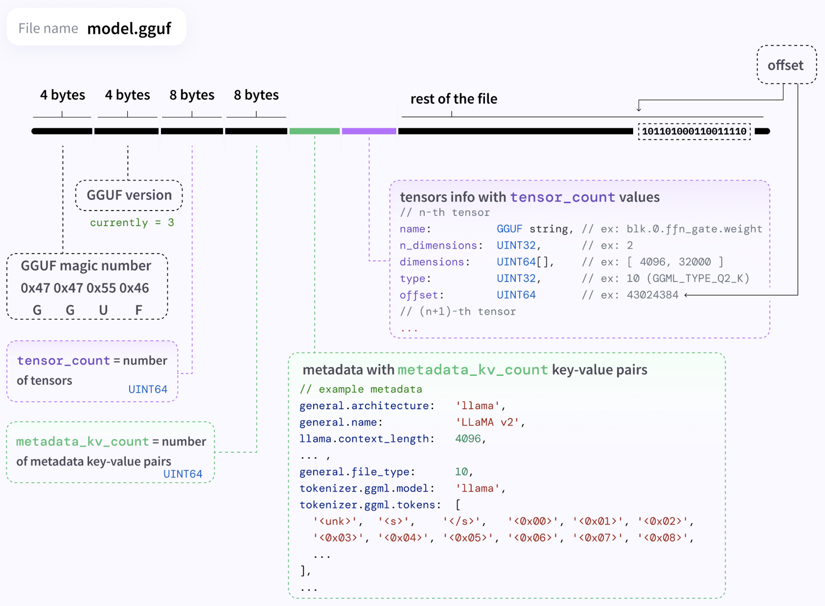
Quantization Types
-
Legacy Quants (\(Q4_0, Q4_1, Q8_0,\) etc.)
- Basic block-based quantization where each 256-weight block is encoded with 4 or 8 bits per weight and one (\(Qx_0\)) or two (\(Qx_1\)) constants for scaling/offset.
- Simple bit-unpacking operations (bit shift, AND, multiply) make these formats highly efficient for older hardware and platforms without vector acceleration.
-
K-Quants (\(Q3_{K_{S}}, Q5_{K_{M}},\) etc.)
- Smarter allocation of bits across layers or weight blocks, guided by internal heuristics or optional importance matrices.
- Uses combinations of quantization levels in different layers (XS, S, M), optimizing performance-quality tradeoff.
- Maintains speed advantages of legacy quants while improving model fidelity and reducing quantization noise.
-
I-Quants (\(IQ2_{XXS}, IQ3_S, IQ4_{XS},\) etc.)
- Advanced block-wise quantization using ideas from QuIP; includes lookup tables to store additional decoding values.
- Allows lower bpw (2-4) while preserving model quality, especially useful for extremely memory-constrained inference.
- Lookup-based dequantization introduces more compute overhead and can cause performance regressions on CPU-bound hardware.
GGUF File Layout and Execution
- Each GGUF file begins with a magic header and version indicator (
0x47 0x47 0x55 0x46for “GGUF”, currently version 3), followed by two 64-bit integers: the number of tensors and number of metadata key-value pairs. - Tensor definitions include name, shape, type, and byte offset. Supported quant types include formats like
GGML_TYPE_Q2_K, \(Q3_K\), or \(IQ4_{XS}\). - Metadata stores tokenizer info, architecture name, context length, and any quantization parameters used during export.
- Tensors are read from disk at inference time via offset pointers—enabling partial loading or memory-mapped inference.
Importance Matrix (Imatrix)
- An optional matrix that prioritizes preserving accuracy in weights deemed most significant based on a calibration pass.
- Can be used with K-quants and legacy quants, not exclusive to I-quants.
- Stored directly in the GGUF metadata and silently improves quantization quality with no inference-time cost.
Pros
- Efficient deployment format: GGUF enables fast loading, lightweight inference, and portable packaging across platforms.
- Flexible quant schemes: From legacy-friendly \(Q8_0\) to ultra-compressed \(IQ2_{XXS}\), GGUF supports a wide range of bit-widths and precision tradeoffs.
- All-in-one packaging: Tokenizers, metadata, and importance matrices are embedded—no need for external configuration files.
- Community driven: Supported natively by
llama.cppand increasingly integrated with Hugging Face tools and runners.
Cons
- Hardware-specific behavior: Some quant schemes (especially I-quants) may perform suboptimally on older CPUs or non-VNNI hardware.
- Naming ambiguity: Quantization method and imatrix usage are not always visible in the filename; may require manual inspection or re-quantization.
- Rapid evolution: Format and tooling are evolving quickly—older GGUF models may need conversion to newer versions.
AWEQ: Activation‑Weight Equalization
- Introduced in AWEQ: Post‑Training Quantization with Activation‑Weight Equalization for LLMs (Nov 2023) by Li et al., AWEQ is a training‑free post‑training quantization technique designed to facilitate both ultra‑low‑bit and 8‑bit weight+activation (e.g., W8A8) quantization in large language models such as Llama and OPT. It works by shifting quantization hardness from activations to weights to reduce error.
- AWEQ effectively balances activation and weight ranges channel-wise via per-channel equalization followed by uniform quantization, incorporating bias correction to reduce residual errors. It achieves significantly improved quantization accuracy—especially for W8A8 floating‑point alternatives—without any training or runtime slow-down, making it an excellent choice for production deployments requiring both efficiency and fidelity.
Motivation
- Large‑scale LLM activations often exhibit long‑tailed per‑channel distributions with large outliers, making activation quantization challenging even at 8 bits. AWEQ addresses this by balancing activation and weight ranges so that differences in range (and therefore quantization difficulty) are harmonized channel‑wise, reducing wastage in the quantization grid and improving uniform quantization performance.
Process (Implementation Overview)
-
Channel Range Analysis
- Run forward passes over a small calibration dataset to compute per‑channel activation range \(r(X)_i = \max(X_i) - \min(X_i)\) and weight range \(r(W)_i\) for each linear or attention block tensor. Range refers to max minus min values across all elements in that channel.
-
Equalization Factor Computation
-
Compute a scale vector \(s \in \mathbb{R}^C\) to equalize ranges via:
\[\tilde{X}_i = \frac{X_i}{s_i}, \quad \tilde{W}_i = s_i \cdot W_i\]- The objective is typically set such that \(r(\tilde{X}_i) = r(\tilde{W}_i)\) for all \(i\), thereby maximizing per‑channel quantization precision as defined through product of normalized ranges (see Equations 3–10 in the original text).
-
-
Tensor Scaling (Fusion)
- Apply channel‑wise scaling at the input boundaries of transformer modules—such as prior to self‑attention key/value/data and FFN layers.
- Merge activation scaling into preceding layers (e.g., LayerNorm or Linear) to eliminate runtime overhead. For example, transform internal \(W \leftarrow \mathrm{diag}(s) \, W\); hence, activations use quantizable ranges without additional scaling logic.
-
Uniform Quantization
- Quantize the equalized tensors using per‑tensor uniform affine quantization (e.g., 4‑bit or 8‑bit symmetric). Activation quantization thresholds can be fused with the input block for efficient inference.
-
Quantization Bias Correction (BC)
- Because quantization after scaling and symmetric clipping can introduce a bias \(\epsilon = W_f - W\), AWEQ applies post‑hoc bias correction:
- where \(\mathbb{E}[x]\) is estimated over calibration data, and \(y_e = (W + \epsilon)x\). This corrects the expected error per layer without changing runtime performance, enhancing stability in deep LLMs without BatchNorm.
Pros
- Training‑free, with no need for quantization-aware training or gradient-based fine-tuning.
- Supports both W8A8 activation quantization and ultra‑low-bit weight-only quantization, including
int/4with robust performance. - Hardware-friendly, as it avoids dynamic scaling during inference; changes are statically fused before deployment.
- Demonstrates best-in-class accuracy on tasks such as zero‑shot Llama 2 7B evaluation (e.g., average: 70.38% over PIQA, HellaSwag, WinoGrande, ARC‑e—all within <0.01 absolute from
float16).
Cons
- Requires representative calibration data to compute statistics and activation range profiles.
- Per‑tensor quantization may not perform as well as per‑channel for certain weight distributions, though the equalization helps mitigate this.
- Slight overhead in computing equalization factors and bias expectations at quantization time (calibration phase only).
EXL2 Quantization
-
ExLlamaV2, commonly known as EXL2, is a flexible, weight-only quantization scheme developed specifically for local inference of large language models on consumer GPUs. It supports mixed-precision quantization with bit-widths from 2 to 8 bits, and can dynamically allocate precision per weight group to optimize model accuracy at a target average bitrate. This makes it suitable for extreme compression of LLMs such as Llama2-70B, enabling execution on GPUs with as little as 24 GB VRAM.
-
EXL2 builds upon the GPTQ framework but introduces finer-grained control over quantization allocation, using an error-minimization strategy driven by calibration data. Unlike uniform quantization, EXL2 allows important weights to retain higher precision while compressing less critical ones more aggressively. This is implemented without significant performance penalties due to tight integration with ExLlama’s inference engine and CUDA backend.
Process
-
Calibration and Error Evaluation:
- Begin by passing a small calibration dataset through the model to obtain representative statistics.
- For each linear layer weight matrix, the EXL2 pipeline quantizes the matrix multiple times using different bit-width configurations (e.g., 2, 3, 4, 5, 6, or 8 bits).
- After each quantization trial, compute the quantization error between the original and quantized matrix multiplied by the calibration input. The maximum per-layer error across all trials is tracked.
-
Bitrate-Constrained Optimization:
- A greedy or grid-based search selects the bit-width assignment that minimizes the maximum layer-wise error while satisfying a user-defined average bitrate target (e.g., 2.55 bits per weight).
- This allows for non-uniform quantization within each matrix, so important rows or columns (typically corresponding to high-magnitude weights or activations) may receive higher precision.
-
Mixed-Bit Packing and Storage Format:
- Each matrix is stored in a compact format supporting mixed-bit representation. A metadata structure encodes the bit-width used for each group.
- Group size is typically fixed (e.g., 64 or 128), enabling compatibility with blockwise CUDA kernels.
- The storage layout ensures efficient memory access and can be interpreted directly by ExLlama’s fast inference kernels.
-
Inference Support:
- At runtime, ExLlamaV2 uses custom CUDA kernels capable of unpacking and computing with mixed-bit quantized weights.
- There is no need for runtime dequantization to full precision—matmul and sampling are done directly on quantized values.
- The system also supports act-order remapping, allowing reordering of weight matrices to preserve activation alignment in grouped attention layers, which is important for compatibility with GQA architectures and inference speed.
-
Conversion Pipeline:
-
A command-line script is provided to convert Hugging Face-format models into EXL2 quantized versions. This script includes:
- Automatic bit-width search using calibration data.
- Weight remapping and act-order alignment.
- Storage into a compact format suitable for ExLlamaV2.
-
Conversion is computationally intensive, especially for large models, but only needs to be done once.
-
Pros
- Extreme compression: Achieves ultra-low bitrates (e.g., 2.5–3.0 bpw) without retraining, enabling 70B models to run on 24 GB GPUs.
- Layer-aware precision allocation: Allocates bits where they matter most, reducing perceptual degradation in output quality.
- Performance-friendly: Designed for fast execution with minimal overhead through mixed-bit CUDA kernels.
- Flexible deployment: Supports a range of bitrates and model sizes, allowing trade-offs between quality and performance.
Cons
- Complex conversion: Requires full model calibration, multiple quantization trials per matrix, and custom tooling.
- Conversion time: Large models (13B–70B) take significant time to convert due to exhaustive per-layer bit-width search.
- Inference compatibility: Requires ExLlamaV2 backend for proper kernel execution; not compatible with standard PyTorch or ONNX runtimes.
SpinQuant
- Introduced in SpinQuant: LLM Quantization with Learned Rotations by Liu et al. (2024), SpinQuant reduces quantization error by applying learned orthonormal rotations to weights, activations, and KV-cache blocks. These rotations normalize tensor distributions, mitigate outliers, and enable accurate W4A4KV4 quantization. The implementation is available on GitHub.
Process
-
Parameterize rotation matrices:
- SpinQuant uses blockwise orthonormal rotation matrices initialized using Hadamard, shortcut, or random orthonormal bases.
- These rotations are applied to groups of weights, activations, and KV-cache blocks (e.g., \(Q\), \(K\), \(V\) matrices or FFN weights), where outliers may exist.
-
Optimize via Cayley-SGD on the Stiefel manifold:
- A small calibration set is passed through a simulated W4A4KV4 pipeline.
- Quantization error (e.g., MSE or KL divergence) between full-precision and quantized outputs is computed.
- Gradients are backpropagated through the rotation parameters using Cayley-SGD, a method that maintains orthonormality constraints by optimizing directly on the Stiefel manifold.
-
Fold optimized rotations into model weights:
- Once optimized, the learned rotation matrices are fused into the model weights and biases (e.g., replacing \(W\) with \(R^T W R\)) during preprocessing.
- This ensures that no extra computation is introduced at inference time—quantization is performed on the already rotated tensors.
-
Apply W4A4KV4 quantization:
- Post-rotation, weights, activations, and KV-cache blocks are quantized to 4-bit using standard uniform quantization schemes.
- The rotations have distributed the influence of large-magnitude outliers, allowing for a tighter and more efficient quantization range.
Pros
-
Outlier mitigation via distribution normalization:
- Rotations “smear” large-magnitude values across dimensions, redistributing peak energies that would otherwise dominate quantization bins.
- This normalization significantly reduces the impact of extreme values and improves low-bit quantization fidelity.
-
Accuracy preservation:
- Achieves within ~2.9 points of full precision on Llama 2 (7B) zero-shot tasks.
- Outperforms existing techniques like AWQ, SmoothQuant, and QuaRot by 19–45% in accuracy retention.
-
No runtime overhead:
- Unlike some quantization techniques that add inference complexity, SpinQuant’s learned rotations are merged offline.
- At inference, the model behaves identically to a standard quantized model, with no additional compute.
Cons
-
Involves optimization and calibration:
- Cayley-SGD optimization introduces computational overhead during preprocessing.
- Requires a small validation set to simulate quantization and compute gradients.
-
Preprocessing complexity:
- Folding rotations into model weights adds engineering complexity, especially when targeting hardware deployment.
- Though folded offline, the rotated tensors may have slightly increased numerical range, requiring careful scale selection.
-
Larger intermediate tensors:
- While inference cost remains low, merged rotated weights can increase storage slightly due to loss of weight sparsity or alignment.
FPTQuant
- Introduced in FPTQuant: 4-bit Function‑Preserving Transforms for Transformer PTQ by Pan et al. (2025), Function-Preserving Transforms Quantization (FPTQuant) reshapes transformer activations before quantization to preserve function.
- A complementary overview is available in Lei Mao’s Log Book.
Process
-
Function-Preserving Activation Transforms:
-
FPTQuant applies mathematically invertible transforms to the activations in attention and feedforward blocks to reduce their dynamic range. These include:
- Logarithmic transforms: Applied to soften the long-tailed distributions (especially in attention scores or MLP activations).
- Affine or exponential transforms: Normalize activations without changing the computation graph logic.
-
-
Merging Transforms into Weights:
- Since these transforms are invertible, the effect can be canceled out by adjusting the downstream linear weights.
-
Specifically:
- Let \(x \rightarrow f(x)\) be the transform applied to activations.
- Then \(Wx \rightarrow Wf^{-1}(f(x))\) ensures the output remains unchanged.
- FPTQuant modifies the linear projection weights accordingly so that the transform step is absorbed and the forward function is preserved.
-
Quantization Step:
- With the dynamic range compressed, 4-bit symmetric per-channel quantization is applied to the adjusted weights using PTQ methods.
- Activations are not explicitly quantized, but their transformed form is compatible with W4A16 runtimes (e.g., vLLM) where only weights are quantized.
-
No Runtime Penalty:
- All transforms are resolved offline and merged into weights.
- The runtime model is a standard quantized model with no extra ops introduced during inference.
Pros
- Fully training-free, invertible, and architecture-agnostic.
- Achieves
int4weight-only quantization with minimal or no accuracy loss, by preserving function through mathematically exact transformation. - Compatible with W4A16 systems like vLLM, delivering significant memory and latency improvements without major architectural rework.
Cons
- Primarily targets weights—does not quantize activations directly, limiting total memory benefits.
- Still an emerging method—performance and generalization are under ongoing validation across LLM variants (e.g., Mistral, Gemma).
- May require per-layer transform tuning based on architecture layout (e.g., attention vs MLP blocks).
Palettization (Weight Clustering)
- Palettization, also known as weight clustering, is a quantization scheme that replaces full‑precision weights with low‑bit indices into a small lookup table (LUT). Each weight value is approximated by the nearest centroid in the LUT, enabling efficient storage and retrieval.
Process
- Clustering: Collect all float‑format weights for a layer (or group of layers), then run k-means clustering to derive a set of centroids (typically, \(2^{n}\) entries for n‑bit palettization).
- Index Mapping: Each weight is replaced with an integer index pointing to its closest centroid in the LUT. The original full‑precision value is no longer stored.
- Granularity Options:
- Per‑tensor granularity: A single LUT for the entire weight tensor.
- Per‑group‑channel granularity: The tensor is divided into groups of channels (defined by
group_size), each with its own LUT—offering a better accuracy/compression trade-off.
- Optional Vector Clustering (
cluster_dim > 1): Enables multi-dimensional centroids by clustering weight vectors instead of scalars, improving approximation quality for some architectures. - Post‑processing: Optionally quantize LUT centroids themselves to a lower precision (e.g.
int8) for additional compression.
Integration in Workflows
- Available via Apple’s
coremltools.optimize.torch.palettizationAPI, which injects FakePalettize layers into the model for palettization-aware training (PAT). - During training, k‑means clustering is applied online, and the LUT and indices are learned through gradient steps. After convergence, the
finalize()call folds LUTs and indices into permanent quantized weights.
When to Use Palettization
- Memory-critical deployment: Edge devices or mobile apps where weight storage is the bottleneck.
- Aggressive compression: Scenarios requiring sub‑4‑bit representation.
- Architecture flexibility: Works with both CNNs and transformers when standard affine quantization struggles.
- Fine‑tunable deployment targets: Fine-tuning after palettization enables high accuracy while still achieving significant compression ratios.
Pros
- Extreme compression: Supports ultra-low bit‑width representations (e.g. 2–4 bits) for weights.
- Memory savings: Offers major memory savings—each weight becomes a small index instead of a float.
- Vector clustering: Multidimensional centroids can preserve structure in weight matrices.
- Flexible granularity: Per-tensor, per-group, or vector-level control enables tailored compression vs. accuracy trade-offs.
- Compatible with fine‑tuning: Compatible via PAT, allowing retention of accuracy through fine‑tuning post-clustering.
Cons
- Requires additional training or fine‑tuning steps (PAT) to compensate for quantization error.
- Clustering and LUT management adds complexity to both training and inference pipelines. In other words, introduces LUT metadata and integer-to-centroid lookup logic in inference.
- Larger runtime overhead than standard affine quantization, especially with per-channel or per-group palettization which increases storage overhead for multiple LUTs and adds runtime logic to look up indices.
- Less intuitive and more complex to implement than simple scale-based quantization.
What to Use When?
-
Selecting the right method depends on deployment goals, model architecture, available compute, and desired trade-offs between accuracy, speed, and memory. Below is a structured guide to help determine what to use when.
-
For Ultra-Low Bit Weight-Only Quantization (
int3/int4) with No Accuracy Drop:-
Use: AWQ, FPTQuant, GPTQ, EXL2, SpinQuant
- AWQ: Best for fast deployment of LLMs (e.g., Llama) on edge GPUs or low-latency inference with prebuilt CUDA kernels. No training or tuning required, and integrates well with TinyChat or similar runtimes.
- FPTQuant: Ideal when you need function-preserving
int4compression with no runtime penalty and full compatibility with transformer architectures. Use for W4A16 deployment in platforms like vLLM. - GPTQ: Recommended for very large models (13B–175B) where preserving perplexity is critical. Use when quantization accuracy is a priority and you’re comfortable with modest compute during conversion.
- EXL2: Choose when running massive models (e.g., Llama2-70B) on consumer GPUs. Offers the best compression-speed balance via dynamic bit allocation and works well with ExLlama.
- SpinQuant: Select when targeting 4-bit quantization of both weights and activations while retaining high accuracy (e.g., for academic or performance-sensitive production use). Best for W4A4KV4 targets with pre-deployment compute budget.
-
-
For Full W8A8 Quantization (Weight + Activation):
-
Use: SmoothQuant, AWEQ
- SmoothQuant: The best choice for training-free, full
int8quantization with minimal setup. Choose for static quantization pipelines on NLP models like Llama, OPT, or BLOOM where CPU or GPUint8inference is desired. - AWEQ: Prefer this over SmoothQuant when you need better accuracy with activation-weight balance, especially for models that are hard to quantize (e.g., with long-tailed distributions). Supports both W8A8 and ultra-low-bit variants, and requires no fine-tuning.
-
-
For Mixed-Precision or Variable-Bitrate Quantization:
-
Use: EXL2, GGUF (K-Quants, I-Quants)
- EXL2: Use when deploying models in memory-constrained environments but still wanting to preserve key model behavior via bit allocation per group. Especially useful for interactive LLMs on laptops or desktops.
- GGUF (K/I-Quants): Ideal for offline, file-efficient packaging and CPU or mobile inference with tooling like
llama.cpp. Offers a trade-off between compatibility and compression via predefined quant profiles (\(Q3_{K_{S}}\), \(IQ4_{XS}\), etc.).
-
-
For Extreme Compression with Customization or Training Support:
-
Use: Palettization (Weight Clustering)
- Use palettization when maximum compression is needed and some fine-tuning is acceptable. Ideal for mobile deployment or experimental architectures where LUTs and centroid representation can drastically reduce size.
- Choose vector clustering when structure preservation in weight matrices matters (e.g., vision-transformer hybrids or customized transformer blocks).
-
-
For Legacy or Format-Constrained Inference:
-
Use: GGUF (Legacy Quants)
- Best suited for lightweight, portable LLM inference on CPU or embedded hardware via
llama.cpp. - Use when you need fast loading, offline conversion, and minimal dependencies, especially for local LLMs or desktop chatbots.
-
-
If Activation Quantization Is Not Required (Weight-Only Models):
-
Use: AWQ, GPTQ, FPTQuant, EXL2
- These methods focus on
int3/4weight-only quantization without modifying activations (typically left infloat16orbfloat16). - Use these when inference memory is not your bottleneck, and you want the best latency-to-accuracy trade-off without model retraining.
-
-
Summary Decision Matrix:
| Goal / Constraint | Recommended Method(s) |
|---|---|
| Fastest low-bit inference (no training) | AWQ, FPTQuant |
| Best W4A4 quantization accuracy | SpinQuant |
| W8A8 quant with balanced scaling | SmoothQuant, AWEQ |
| Largest models on smallest VRAM | EXL2, GPTQ |
| Mixed precision with dynamic control | EXL2, GGUF (K/I-Quants) |
| CPU/mobile inference with format support | GGUF |
| Edge deployment with low compute budget | AWQ, GGUF (Legacy) |
| Extreme compression + retraining allowed | Palettization |
| Activation-aware optimizations | SpinQuant, SmoothQuant, AWEQ |
Comparative Analysis
| Method | Type | What Quantized | Bits | Training-Free? | Key Innovation | Accuracy Retention | Introduced |
|---|---|---|---|---|---|---|---|
| Uniform Quantization | Post Training Quantization | Weights ± Activations | 4–8 bit | yes | Simple affine mapping, per-tensor or per-channel | Good for smooth distributions (~2pt drop) | (Fundamental baseline) |
| GPTQ | Post Training Quantization | Weights only | INT3/4 (also 2-bit) | yes | Second-order Hessian-based error compensation per-layer | Highly accurate (perplexity within ~0.03 of float16) |
Oct 2022 |
| SmoothQuant | Post Training Quantization | Weights + Activations | W8A8 | yes | Scaling activation/weights to balance quantization difficulty | Very high (<0.5 % loss) | Nov 2022 |
| AWQ | Post Training Quantization | Weights only | W4 | yes | Activation-aware per-channel scaling via calibration | High (>float16) |
Jun 2023 |
| GGUF | Post Training Quantization | Weights only | 2–8 bit (block-based) | yes (quantized offline) | Flexible binary format with various schemes, importance matrices embedded | Varies by scheme; efficient loading | Aug 2023 (as part of `llama.cpp`) |
| AWEQ | Post Training Quantization | Weights + Activations | W4 or W8A8 | yes | Activation-weight equalization + bias correction | Best-in-class (within <0.01 absolute from float16) |
Nov 2023 |
| EXL2 (ExLlamaV2) | Post Training Quantization (dynamic allocation) | Weights only | Mixed: 2–8 bit | yes | GPTQ-based mixed-bit allocations per layer via error minimization | Very high; Llama2-70B runs on 24 GB GPU | Nov 2023 |
| SpinQuant | Quantization Aware Training (calibration + optimization) | Weights + Activations + KV-cache | W4A4KV4 | no (requires calibration + optimization) | Learned orthonormal rotations to normalize distributions | Within ~2.9 pt of FP | May 2024 |
| FPTQuant | Post Training Quantization | Weights only | W4 (weight-only) | yes | Function-preserving invertible transforms to activations, merged into weights | Excellent (minimal loss) | Jun 2025 |
| Palettization | Quantization Aware (Training or Fine-tuning) | Weights only | 2–4 bit (LUT index) | no (requires fine-tuning or PAT) | Weight clustering via k-means with optional vector or group granularity | High (with PAT); moderate otherwise | 2024 |
Multimodal Quantization
- Quantizing multimodal LLMs—especially Vision-Language Models (VLMs) such as BLIP-2, LLaVA, or Flamingo—presents unique complexities not encountered in traditional text-only LLMs. These models process and fuse inputs from disparate modalities (e.g., images and text), resulting in heterogeneous model architectures and dynamic activation distributions that resist uniform quantization techniques.
- The inherent heterogeneity in architecture, distribution, and task metrics makes naive post-training quantization insufficient for production-grade deployment. Mixed-precision and QAT remain the most promising paths forward, especially when combined with robust calibration data and modality-aware loss functions. As VLMs become more prevalent in edge AI and on-device inference, a new generation of quantization-aware toolchains will be essential to unlock their full potential.
Why VLM Quantization Is More Complex
-
Multimodal models are composed of at least two distinct processing pipelines—one for each modality (e.g., image and text)—and often a third for cross-modal alignment or fusion. This architectural heterogeneity introduces the following challenges:
- Diverse tensor statistics: Vision and language inputs yield activations with vastly different distributions and dynamic ranges, making uniform quantization impractical across modalities.
- Cross-modal attention sensitivity: Cross-attention layers that fuse modalities are especially fragile to precision loss, as they are responsible for preserving semantic alignment between vision and language.
- Embedding alignment: Vision embeddings (e.g., image patches from ViTs) and text embeddings must remain aligned for effective fusion. Quantization artifacts can easily disrupt this shared embedding space.
- Lack of inductive biases: Unlike CNNs, which offer natural robustness to quantization via spatial weight sharing and locality, ViTs and transformers often rely more heavily on learned long-range dependencies, which are easily degraded by quantization noise.
- Multi-objective optimization: A VLM may be used across many tasks (e.g., captioning, VQA, grounding), requiring quantized models to generalize well across domains, not just on language metrics like perplexity.
-
To address these challenges, quantization of multimodal models typically involves hybrid and adaptive strategies as described below.
Quantizing the Visual Backbone
-
CNN-based encoders (e.g., ResNet, EfficientNet):
- CNNs are relatively robust to quantization, and standard per-channel
int8quantization (as used in MobileNet) can often be applied. - Pre-trained encoders may be frozen and quantized independently of the rest of the model.
- CNNs are relatively robust to quantization, and standard per-channel
-
Vision Transformers (ViTs):
- More sensitive to quantization due to their reliance on attention mechanisms and lack of inductive biases.
- Key operations such as softmax and positional embeddings are particularly fragile.
- Attention maps are harder to compress as they carry spatial relevance crucial for image understanding.
Best practices:
- Use per-head or per-channel quantization for attention weights.
- Apply post-training quantization (PTQ) carefully, or use quantization-aware training (QAT) for attention-heavy layers.
- Maintain FP16 or BF16 precision in early layers or attention blocks if task-critical.
Quantizing the Language Backbone
-
Language processing in VLMs is typically transformer-based (e.g., LLaMA, T5, GPT-style decoders). The quantization techniques here are more mature and generally follow:
int8orint4quantization using post-training methods (e.g., GPTQ, AWQ, SmoothQuant).- Per-group or per-channel quantization for MLPs and attention blocks.
- Mixed-precision inference, especially keeping attention output or layer norms in FP16 when accuracy is crucial.
Cross-Modal Projection and Fusion Layer Quantization
-
This is the most critical and fragile component in VLMs. The fusion modules align visual and textual embeddings into a shared latent space.
- Cross-attention layers are highly sensitive to quantization because they match image regions with textual tokens. Errors here degrade the entire model’s reasoning ability.
-
Query Transformers (Q-formers), as used in BLIP-2, process image features into language-style prompts. Quantization here must preserve alignment fidelity.
-
Strategies:
- Retain cross-modal fusion (specifically, projection and/or cross-attention layers) in FP16 or use higher-precision
int8. - Apply QAT to cross-modal components to preserve alignment under quantization-induced rounding and clipping.
- Use per-tensor calibration based on multimodal datasets to balance activations across modalities.
- Retain cross-modal fusion (specifically, projection and/or cross-attention layers) in FP16 or use higher-precision
Quantization-Aware Training (QAT) in VLMs
-
Due to sensitivity in fusion and vision branches, QAT is often required for VLMs, unlike in pure-text LLMs where PTQ often suffices.
- During QAT, fake quantization layers simulate precision loss during both forward and backward passes.
-
Loss functions may include:
- Cross-modal alignment loss (cosine similarity of vision/text embeddings)
- Task-specific loss (e.g., VQA classification loss)
- KL divergence or logit-matching between full-precision and quantized models
-
Progressive QAT approaches are sometimes used:
- Freeze the vision encoder
- Apply quantization noise gradually to fusion layers
- Fine-tune using diverse tasks to preserve robustness
Calibration and Evaluation in VLMs
-
Calibration datasets for VLMs must reflect the multimodal distribution. Suitable datasets include:
- MS-COCO (captioning)
- VQAv2 (VQA)
- GQA, VizWiz, RefCOCO (referring expression comprehension)
-
Metrics to evaluate quantized VLMs differ from those used in text-only LLMs:
- Captioning: CIDEr, BLEU, METEOR
- VQA: answer accuracy
- Localization: IoU and precision
-
These tasks are affected differently by quantization; degradation in fusion modules typically leads to sharper accuracy drops than in text-only settings.
Hybrid and Mixed-Precision Quantization
- Given the disparity in sensitivity across components:
- Use
int8orint4for robust modules (e.g., MLPs, FFNs) - Use FP16 or BF16 for:
- Cross-modal projections
- Final projection
- Optionally, try attention output and embedding normalization layers
- Use
- Mixed-precision kernels in deployment frameworks (e.g., TensorRT, OpenVINO) allow selective high-precision execution.
Tooling Support
-
Quantization tooling for VLMs is still developing. While text-only LLMs enjoy mature and well-integrated support in libraries like GPTQ and AWQ, multimodal quantization often requires combining custom workflows with early-stage tooling.
-
Current options include:
-
TensorRT: NVIDIA’s inference engine supports mixed-precision ViT and fusion models with custom kernels for
int8and FP16. Requires ONNX export and hardware-specific calibration. -
OpenVINO: Intel’s deployment toolkit for CPU/GPU/VPUs. Supports post-training quantization and VLMs exported via ONNX or Hugging Face pipelines.
-
Hugging Face Optimum: A library bridging Transformers with hardware backends. Supports quantization workflows with Intel Neural Compressor and ONNX Runtime for vision+language models.
-
Intel Neural Compressor: An open-source tool for quantization (PTQ, QAT, dynamic) across PyTorch and TensorFlow. Early support for multimodal calibration and per-layer configuration.
-
LLaVA Quantized Forks: Some forks of LLaVA apply GPTQ-style
int4quantization to the language backbone. However, the vision encoder and fusion modules are often left in FP16 due to sensitivity. -
BLIP-2 Quantized Implementations (via LAVIS): Some unofficial variants quantize the visual backbone and language decoder separately, relying on hybrid strategies. The Q-former is often kept in higher precision.
-
Emerging research tools are adapting GPTQ and AWQ to support VLMs, although these approaches require careful per-layer calibration and fine-tuning with multimodal datasets.
-
Note: As of now, there is no unified framework for full-stack VLM quantization (vision encoder, fusion, and decoder) akin to what exists for LLaMA or GPT models. Most implementations involve manually freezing or partially quantizing the model.
Comparative Analysis of LLMs vs. VLM Quantization
| Component | Text LLM (e.g., GPT) | VLM (e.g., BLIP-2, LLaVA) |
|---|---|---|
| Architecture | Uniform transformer | Heterogeneous (ViT + LLM + cross-attn) |
| Sensitivity to quant. | Moderate | High (esp. fusion layers) |
| Common quant methods | PTQ, QAT, GPTQ, AWQ | Mixed-precision, QAT, PTQ (limited) |
| Vision encoder | N/A | CNN/ViT, sensitive to int4/int8 |
| Cross-modal fusion | N/A | Needs higher precision |
| Evaluation metric | Perplexity | Task-specific (e.g., VQA accuracy) |
| Tooling maturity | High | Low to medium |
Device and Operator Support across Frameworks
PyTorch
-
Quantization in PyTorch is supported for a limited subset of operators, and the availability of these operators depends on the specific quantization approach being employed—dynamic, PTQ, or QAT. The list of supported quantized operators is not exhaustive and evolves with newer PyTorch releases. For an up-to-date reference, consult the official PyTorch quantization documentation here.
-
The implementation of quantization in PyTorch is backend-dependent, meaning that both the quantization configuration (which defines how tensors are quantized) and the set of quantized kernels (which define how arithmetic is performed on quantized tensors) vary based on the target hardware. Currently, PyTorch provides official support for quantized inference only on CPUs, specifically for x86 and ARM architectures. These are supported via two primary backends:
fbgemm: Optimized for server-class x86 CPUs.qnnpack: Designed for mobile ARM CPUs.
-
The backend must be explicitly set to ensure compatibility between the model’s quantized representation and the runtime kernels, as shown in the example below:
import torch backend = 'fbgemm' # 'qnnpack' for ARM/mobile inference my_model.qconfig = torch.quantization.get_default_qconfig(backend) # Prepare and convert model # Set the backend on which the quantized kernels need to be run torch.backends.quantized.engine = backend # Continue with model preparation and conversion steps... -
QAT in PyTorch is performed in full-precision (
float32) mode to leverage existing GPU or CPU hardware during training. This technique simulates the effects of quantization during training to improve model robustness when deployed with quantized weights. QAT is particularly beneficial for convolutional neural networks (CNNs), especially lightweight models such as MobileNet, where static or dynamic post-training quantization may result in unacceptable accuracy degradation.
Integration in torchvision
-
The
torchvisionlibrary includes integrated support for quantization in several widely used neural network architectures. These include GoogLeNet, InceptionV3, ResNet (various depths), ResNeXt, MobileNet (V2 and V3), and ShuffleNet. The support is provided in three distinct forms to enable a range of workflows:- Pre-trained quantized model weights: These models are fully quantized and can be used directly for inference without additional fine-tuning.
- Quantization-ready model definitions: These are versions of the models with quantization stubs pre-inserted, making them suitable for post-training quantization or QAT.
- QAT scripts: Scripts are available to perform QAT on supported models. While these scripts are applicable to all the models listed above, empirical evaluations show that QAT tends to yield significant accuracy benefits primarily for lightweight models like MobileNet.
-
Here’s a dedicated tutorial demonstrating how to perform transfer learning with quantization using pre-trained models from
torchvision. This enables developers to take advantage of quantized inference while still adapting models to custom datasets and deployment scenarios.
Resources
- To get started on quantizing your models in PyTorch, start with the tutorials on the PyTorch website.
- If you are working with sequence data, start with…
- If you are working with image data then we recommend starting with the transfer learning with quantization tutorial. Then you can explore static post training quantization.
- If you find that the accuracy drop with post training quantization is too high, then try quantization aware training.
TensorFlow
-
Quantization support in TensorFlow is primarily centered around deployment through TensorFlow Lite (TFLite). Only a subset of TensorFlow operations are supported in quantized form when converting models to run efficiently on edge devices. For a comprehensive list of quantization-compatible operators, refer to the official TFLite operator compatibility documentation here.
-
Quantized inference in TensorFlow is enabled through TensorFlow Lite (TFLite) delegates, which provide optimized execution across various hardware backends. These include:
- CPU Delegate: Supports
int8andfloat16quantized models using XNNPack kernels, which are enabled by default in modern TFLite runtimes. - GPU Delegate: Accelerates inference on mobile and embedded GPUs. It supports
float16quantization and, in limited cases,int8precision. The delegate is available on both Android and iOS platforms. - NNAPI Delegate (Android only): Interfaces with on-device hardware acceleration drivers. Quantized
int8models are typically supported and can see performance improvements depending on the device and vendor-specific drivers. -
Edge TPU Delegate: Targets Google’s Coral hardware and supports only fully integer quantized models with
int8weights and activations. Due to strict operator and quantization constraints, models must be carefully converted and then compiled using the Edge TPU Compiler. - The level of operator support and performance characteristics differ by delegate. For example, the Edge TPU requires that all operations be quantized and supported by its limited op set. Any unsupported operations will result in compilation failure or will require fallback to CPU, which can significantly affect performance. As such, developers must validate operator compatibility prior to deployment by reviewing the TFLite ops compatibility guide and testing with their target delegate.
- CPU Delegate: Supports
-
QAT in TensorFlow is implemented using the
tfmot.quantization.keras.quantize_modelAPI available through the TensorFlow Model Optimization Toolkit (TFMOT). Similar to PyTorch, QAT in TensorFlow is performed in floating point, allowing the model to simulate quantized behavior during training while still leveraging GPU acceleration. This helps preserve accuracy for models that do not respond well to post-training quantization, such as compact architectures like MobileNet or custom CNNs. The general trade-offs between PTQ and QAT in TensorFlow align closely with those in PyTorch, although some feature and operator support mismatches still exist between the two frameworks. -
When using post-training quantization or QAT, it’s important to validate that all critical model operations are supported in TFLite with quantized equivalents. Unsupported operations may be automatically left in float, potentially degrading the intended performance benefits of quantization.
Integration in tf.keras.applications
-
While TensorFlow does not provide pre-quantized models in
tf.keras.applications, the Model Optimization Toolkit provides utilities to quantize these models post-training or prepare them for QAT. Developers can load a model fromtf.keras.applications, apply quantization via TFMOT, and then convert it to TFLite. The process typically involves:- Cloning the model with quantization-aware layers using
quantize_model. - Fine-tuning the quantized model if needed.
- Converting the trained model to TFLite using the TFLiteConverter.
- Cloning the model with quantization-aware layers using
-
TFLite provides tools and guidelines for performing transfer learning with quantized models, though, as with PyTorch, QAT tends to be necessary mainly for accuracy-sensitive lightweight models.
Resources
-
TensorFlow’s PTQ techniques are detailed in the post-training quantization guide.
-
QAT is covered in the QAT guide.
CoreML
-
Quantization support in CoreML is integrated directly into the CoreML Tools conversion pipeline. Quantization can be applied during model conversion from popular frameworks (such as PyTorch or TensorFlow) to the
.mlmodelformat using the coremltools Python API. The supported quantization schemes are primarily weight-only quantization, with formats including:-
float16: Reduces the precision of weights from 32-bit floating point to 16-bit floating point. This is the most common and widely supported quantization type for CoreML, offering significant reductions in model size with minimal accuracy loss. In many cases, Apple hardware (e.g., A-series and M-series chips) executes GPU computations natively infloat16, sofloat16quantization primarily benefits memory footprint and model loading speed rather than raw compute throughput. -
Linear
int8Weight Quantization: Supported through offline quantization incoremltools, mapping weights from float to signed 8-bit integers. This reduces storage and potentially improves memory bandwidth efficiency, but operations are still executed infloat16orfloat32internally on GPU/CPU/NPU. Operator and backend support forint8quantization is more limited compared tofloat16. -
Custom bit-width quantization: Experimental support exists for 4-bit and other weight-only schemes via coremltools compression APIs, but these formats require manual handling and may only run on the CPU backend.
-
-
Post-training quantization (PTQ) in CoreML is performed by passing additional parameters to
coremltools.convertor applying thecoremltools.models.neural_network.quantization_utilsmodule to an existing.mlmodel. For example,float16weight quantization is typically invoked as:import coremltools as ct model = ct.convert( traced_model, convert_to="mlprogram", compute_units=ct.ComputeUnit.ALL ) quantized_model = ct.models.neural_network.quantization_utils.quantize_weights(model, nbits=16) quantized_model.save("model_float16.mlmodel") -
CoreML does not currently provide a native, framework-integrated Quantization-Aware Training (QAT) pipeline equivalent to TensorFlow Model Optimization Toolkit or PyTorch’s QAT modules. Instead, QAT must be performed in the source framework prior to export, and the resulting quantization parameters must be preserved during conversion—if the target CoreML format and operators support them. In practice, this is mostly applicable to simulated
float16or weight-clipped models, as CoreML conversion generally re-encodes models in its own quantization formats. -
Hardware execution backends in CoreML include:
- CPU: Executes in
float32orfloat16, with weight-onlyint8quantization supported in some cases. - GPU: Primarily executes in
float16precision.float16weight quantization typically does not change GPU arithmetic precision but reduces memory usage. - Apple Neural Engine (ANE): Supports some
int8operations and mixed-precision execution. Operator coverage for quantizedint8is limited and depends on both CoreML runtime version and the specific ANE generation.
- CPU: Executes in
-
Developers should verify operator compatibility after quantization, as unsupported quantized layers will be automatically dequantized and executed in higher precision, potentially negating performance or memory savings. The CoreML Tools documentation on quantization provides detailed guidance on supported modes and API usage.
Integration with PyTorch and TensorFlow Models
-
When converting PyTorch models to CoreML using
torch.jit.traceortorch.jit.script, quantization should generally be applied during or after conversion viacoremltoolsrather than relying on PyTorch’s native quantization formats, as these may not be mapped directly to CoreML equivalents. -
TensorFlow models exported via SavedModel or TFLite can be converted to CoreML, but quantized TFLite
int8models are usually re-encoded infloat16orfloat32in the final.mlmodelunless explicitly mapped to CoreML’s weight-onlyint8quantization. -
In both cases, the recommended process for
float16quantization is:- Train or fine-tune the model in the source framework.
- Export to an intermediate format (TorchScript, ONNX, SavedModel).
- Convert to CoreML using
coremltools.convert. - Apply
float16weight quantization viaquantize_weights. - Validate model accuracy and operator execution backend in Xcode or using the CoreML runtime.
Resources
JAX
-
Quantization support in JAX is not built directly into the core library, as JAX is designed to be a high-performance array computation framework with a functional API and just-in-time (JIT) compilation through the XLA compiler (Accelerated Linear Algebra). Instead, quantization workflows in JAX are implemented through external libraries and ecosystem tools that target specific hardware backends. Prominent examples include:
- Flax: A neural network library for JAX that provides high-level model definitions but does not offer native quantization APIs. Quantization is typically performed by integrating Flax models with downstream compilers or deployment toolchains.
jax.laxand custom lowering to XLA: Developers can manually simulate quantization during training by inserting quantization and dequantization operations usingjax.laxprimitives. These operations are compiled into the XLA graph and can be mapped to quantized kernels if the target backend supports them.-
External compilers:
- TensorFlow Lite via
jax2tf: Models written in JAX can be converted to TensorFlow usingjax.experimental.jax2tf, and then quantized using TFLite’s post-training or QAT pipelines. - XLA backends for TPU/CPU: Some integer-based execution paths are available for TPUs through XLA, but these are not exposed as a stable, user-facing quantization API in JAX.
- OpenXLA / IREE: Experimental support exists for lowering JAX computations to IREE, which can target
int8quantized inference on specific accelerators (e.g., Vulkan, CPU, GPU).
- TensorFlow Lite via
-
Because JAX itself does not provide a quantized operator registry, operator support for quantized execution depends entirely on the downstream backend. For example:
- When exporting to TFLite, the available quantized ops match those documented in the TFLite operator compatibility guide.
- When compiling to
XLA:TPUorXLA:CPU, support for integer quantization is highly backend-specific and often limited to linear and convolution operations. - On GPUs, JAX generally runs computations in
float16orbfloat16for mixed-precision training/inference, rather than integer quantization.
-
Quantization-Aware Training (QAT) in JAX is typically implemented manually, as there is no built-in helper API equivalent to PyTorch’s
torch.quantizationor TensorFlow’s TFMOT. The common workflow is:- Insert fake quantization nodes (scale + round + clip) into the model during training to simulate integer precision effects.
- Train the model using JAX transformations (
jit,grad,pmap) as usual, with quantization simulation integrated into the forward pass. - Export the trained model to a backend that supports true integer quantized kernels (e.g., TFLite or IREE).
- This approach requires careful control over numerical ranges and scale factors, which are not automatically managed by the framework.
-
Hardware backend considerations for quantized JAX models:
- CPU (
XLA:CPU): Can execute integer operations if the compiled XLA graph contains integer kernels, but fullint8operator coverage is limited compared to float execution. - TPU (
XLA:TPU): Supportsint8matmul and convolution on newer TPU architectures, but model preparation for TPU quantization requires manual lowering. - GPU (
XLA:GPU): Typically favorsfloat16/bfloat16mixed-precision execution. Integer quantization is not a standard deployment path. - Edge/Embedded: Usually requires exporting to TFLite or another inference framework; quantization support and operator coverage then depend entirely on that target runtime.
- CPU (
Integration Examples
-
Exporting JAX models for quantized deployment via TFLite:
import jax import jax.numpy as jnp from jax.experimental import jax2tf import tensorflow as tf # Define a simple JAX function def model(params, x): w, b = params return jnp.dot(x, w) + b params = (jnp.ones((4, 4)), jnp.zeros((4,))) tf_model = tf.function( jax2tf.convert(lambda x: model(params, x), with_gradient=False), input_signature=[tf.TensorSpec([None, 4], tf.float32)] ) # Convert to TFLite with quantization converter = tf.lite.TFLiteConverter.from_concrete_functions([tf_model.get_concrete_function()]) converter.optimizations = [tf.lite.Optimize.DEFAULT] tflite_quant_model = converter.convert() -
Manual QAT simulation in JAX:
def fake_quant(x, scale, bits=8): qmin = -(2**(bits - 1)) qmax = (2**(bits - 1)) - 1 x_scaled = x / scale x_rounded = jnp.clip(jnp.round(x_scaled), qmin, qmax) return x_rounded * scale- This kind of manual fake-quant insertion is common when prototyping QAT in JAX.
Resources
- jax2tf Documentation – Guide to converting JAX functions to TensorFlow for deployment.
- Flax Documentation – JAX-based neural network library (does not provide quantization directly).
- TFLite Quantization Guide – Relevant for JAX models exported via TensorFlow.
- OpenXLA Project – Future direction for cross-framework compilation, including quantization support.
Choosing the right quantization approach
-
The choice of which scheme to use depends on multiple factors:
- Model/Target requirements: Some models might be sensitive to quantization, requiring QAT.
- Operator/Backend support: Some backends require fully quantized operators.
-
Currently, operator coverage in PyTorch is limited and may restrict the choices listed in the table below. The table below from PyTorch: Introduction to Quantization on PyTorch provides a guideline.
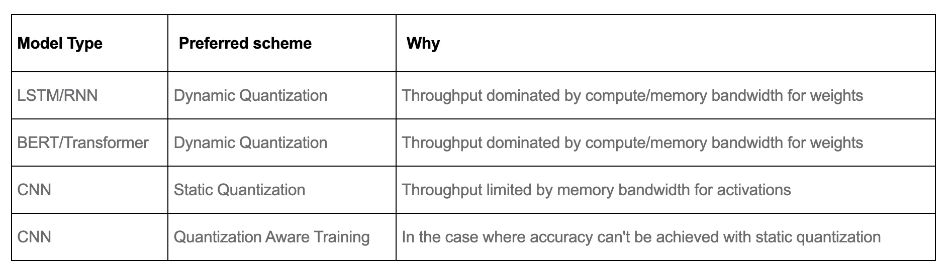
Performance Results
- The table below from PyTorch: Introduction to Quantization on PyTorch offers some sample results:
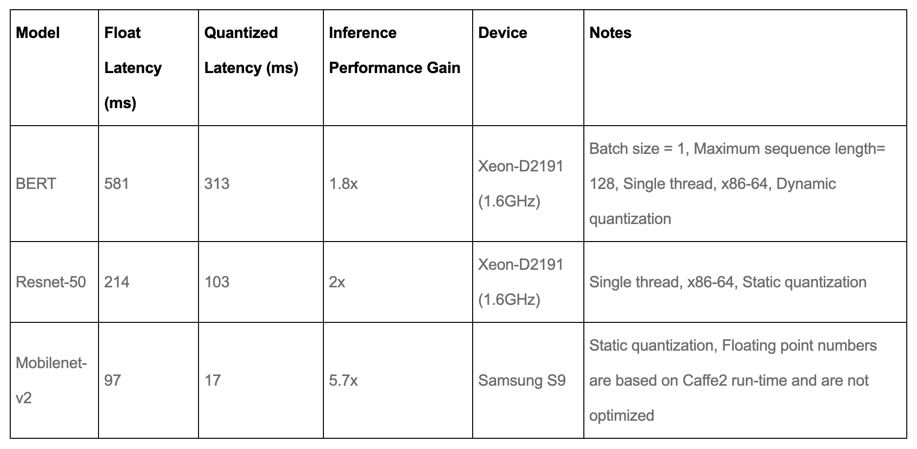
- As seen in the table above, quantization yields a substantial reduction in both model loading time and memory footprint, driven by the 4× smaller model size compared to floating-point implementations. Furthermore, it offers a speedup of 2× to 3× compared to floating-point implementations, depending on the hardware platform and the model being benchmarked.
Accuracy results
- The tables below from PyTorch: Introduction to Quantization on PyTorch compares the accuracy of static quantized models with the floating point models on Imagenet. For dynamic quantization, we compared the F1 score of BERT on the GLUE benchmark for MRPC.
Computer Vision Model accuracy
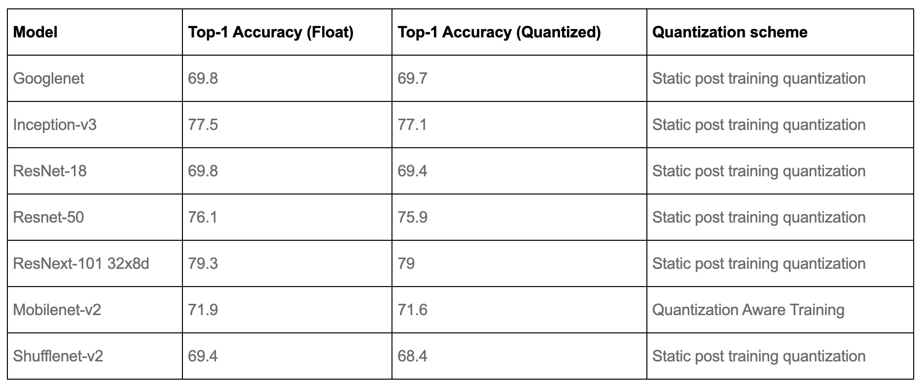
Speech and NLP Model accuracy
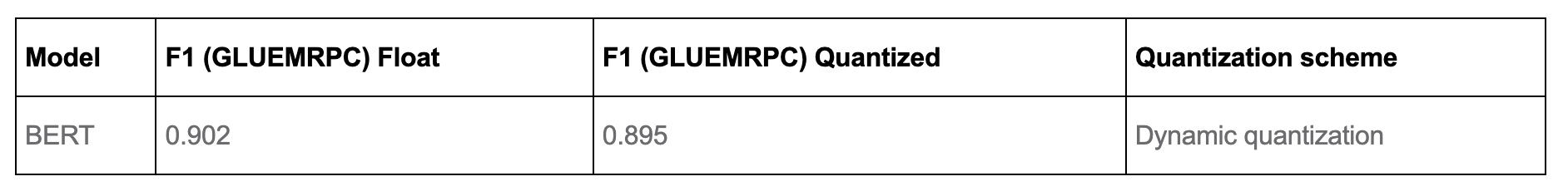
Popular Quantization Libraries
- This section surveys widely used quantization libraries you’ll encounter in practice, what precision/algorithms they support, how they integrate with common stacks, and caveats that matter on-device or in production.
BitsAndBytes
-
BitsAndBytes is a CUDA-accelerated library for low-bit matrix multiply and optimizers. It popularized
LLM.int8(), which uses vector-wise 8-bit quantization but routes “outlier” channels through higher precision matmuls, preserving accuracy while halving memory. It also provides 4-bit weight types used by QLoRA (NF4/float4), plus 8-bit optimizers. In Transformers you typically pass a BitsAndBytesConfig (load_in_4bitorload_in_8bit,bnb_4bit_quant_type="nf4"or"fp4",bnb_4bit_use_double_quant, andbnb_4bit_compute_dtypefor BF16/FP16 accumulation). -
Typical usage (Transformers):
- Construct BitsAndBytesConfig with
load_in_4bit=Trueand your preferred compute dtype (often BF16 for stability) - Load the model with
device_map="auto"` to shard to available GPUs/CPU if needed - When merging adapters back into base weights, dequantize before merging to avoid rounding artifacts, then requantize.
- Construct BitsAndBytesConfig with
-
Notes and caveats:
LLM.int8is weight-only at matmul inputs; activations remain FP16/BF16, so runtime memory isn’t halved unless your serving stack fuses kernels well.- Performance varies by kernel/backend (CUDA vs. ROCm); vendor guides show the expected bottlenecks and setup.
Hugging Face Optimum
-
Optimum is a meta-tooling layer that wraps several backends and exposes unified quantization APIs.
- Optimum ONNX Runtime: PTQ/QAT flows via ORTConfig/ORTQuantizer; supports dynamic (weights int8, activations at runtime), static/QLinear/QDQ with calibration, and QAT. Target for CPU, some NPUs, and cross-platform packaging.
- Optimum Intel (OpenVINO): hooks into NNCF for
int8PTQ and QAT; good CPU/iGPU latency and small memory footprint; provides export to OpenVINO IR and pipeline examples for LLMs. - Optimum Quanto: a PyTorch quantization backend that supports linear quantization of weights to float8, int8, int4, and even int2; works in eager mode, supports QAT, is device-agnostic, and integrates with torch.compile. Great for quick per-module weight-only experiments.
- Optimum Habana (Gaudi): integrates Intel Neural Compressor flows to enable
float8/uint4inference/training paths on HPU. - Transformers integration summary: Transformers supports AWQ, GPTQ, and bitsandbytes out-of-the-box; Optimum layers sit on top to add ORT/OpenVINO/Quanto/TensorRT flows.
ONNX Runtime Quantization
-
ONNX Runtime implements 8-bit linear quantization with scale and zero-point per tensor or per channel, using either static calibration or dynamic quantization. The core mapping follows \(x_\mathrm{fp32} = s \cdot (q - z)\); APIs include
quantize_dynamic,quantize_static(with calibration), andquantize_qat(for QAT-authored models). -
Why choose ORT: stable operator coverage, portable deployment as a single ONNX artifact, and strong CPU performance. Use when you want one model to run across x86/ARM servers and many NPUs with the same runtime.
NVIDIA TensorRT / TensorRT-LLM
-
TensorRT provides PTQ (with explicit quantization replacing older calibration APIs) and supports QAT. TensorRT-LLM adds LLM-specific kernels and recipes:
float8/float4,int4AWQ, andint8SmoothQuant, plus inflight batching and paged KV cache for high throughput. Use TensorRT-LLM when serving NVIDIA-GPU LLMs with low latency at scale. -
Practical tip: for
int8LLMs on NVIDIA GPUs, SmoothQuant (W8A8) with per-channel weight and per-tensor activation scales is a common “safe” baseline; for weight-only speedups, AWQ (W4A16) is widely supported.
Intel Neural Compressor (INC)
- INC is a framework-agnostic toolkit (PyTorch, TensorFlow, ONNX Runtime, MXNet) offering PTQ, QAT, tuning strategies, and hardware-aware search for accuracy/latency/size trade-offs. It’s also the quantization backend used by several Optimum integrations (e.g., Gaudi). Use INC to automate calibration and accuracy recovery across Intel hardware.
OpenVINO Tooling
- OpenVINO provides NNCF-based post-training
int8quantization and QAT, strong CPU/iGPU kernels, and file-size/runtime wins for NLP and CV. Workflows include simple PTQ with a small calibration set and hybrid schemes (e.g., MatMul/Embedding weight-only + activationint8elsewhere). Good match for desktop/server CPUs and integrated GPUs.
TensorFlow Lite
- TFLite supports dynamic range, full-integer (
int8) PTQ,float16weight compression, and QAT, with a well-specified int8 scheme (two’s complement; per-tensor/axis). Choose when deploying to mobile/embedded via NNAPI/Metal/Vulkan delegates.
Apple Core ML Tools
- Core ML Tools supports weight-only linear quantization and palettization (weight clustering into a LUT) with palettization-aware training APIs that insert fake-quant/palette layers during fine-tuning, then fold them into compact weights at export. Use for native iOS/macOS deployments.
LLM-Specific Quantizers (GPTQ, AWQ) and their Python toolkits
- GPTQ (weight-only, usually 4-bit): popular for LLMs; Optimum exposes a GPTQQuantizer, and Transformers documents a GPTQModel path. Note AutoGPTQ was archived in 2025; newer stacks may use GPTQModel via Transformers/Optimum.
- AutoAWQ (AWQ implementation, W4A16): easy 4-bit quantization with fast kernels and wide model coverage; integrates with vLLM and various executors.
Rules of Thumb for Choosing a Library
- If you’re serving NVIDIA-GPU LLMs at scale: start with TensorRT-LLM (SmoothQuant W8A8, or AWQ W4A16), then tune.
- If you need portable CPU inference or a single artifact for many devices: export to ONNX and quantize with ONNX Runtime (static/QDQ).
- If you want the fastest “drop-in” memory cut for HF models on a single GPU: bitsandbytes (
LLM.int8orNF4) via Transformers. - If you target Intel CPUs/iGPUs or want accuracy-constrained auto-tuning: Optimum Intel with NNCF or bare INC.
- If you need pure-PyTorch experimentation across devices with minimal graph rewriting: Optimum Quanto for weight-only quantization (including float8/int4/int2).
- If you deploy to mobile: TFLite (Android) or Core ML Tools (iOS/macOS).
Implementation Notes
- Calibration for static/PTQ: for ORT/OpenVINO/TensorRT
int8, pass a representative dataset; a few hundred samples often suffice for stable scales. - Algebra and mapping: the linear quantizer in ORT and many toolkits uses \(x = s \cdot (q - z)\). Keep \(s>0\), and prefer per-channel scales for weights in matmuls/convs to reduce error.
- Mixed precision realities: many “weight-only” schemes still do FP16/BF16 accumulations; end-to-end memory reduction depends on your kernel fusion and runtime (vLLM/TensorRT-LLM/etc.).
- Library status: GPTQ tooling has shifted; AutoGPTQ is archived—prefer the GPTQModel path in Transformers/Optimum for forward-compatibility.
How Far Can Quantization Be Pushed?
-
Quantization can, in theory, be reduced to a single bit per parameter, enabling what are known as binary neural networks (BNNs). In such models, both weights and, in some cases, activations are constrained to binary values (e.g., {−1, +1}), achieving the most extreme point on the accuracy–performance trade-off spectrum. Several notable research efforts have explored this concept, including:
- BinaryConnect (Courbariaux et al., 2015) – Introduced the idea of training networks with binary weights while retaining full-precision activations.
- XNOR-Net (Rastegari et al., 2016) – Extended the approach by binarizing both weights and activations, and introducing scaling factors to reduce the accuracy drop while enabling efficient bitwise operations.
- XNOR-Net++ (Bulat & Tzimiropoulos, 2019) – Improved upon XNOR-Net through better gradient approximation techniques and optimized binarization strategies, achieving state-of-the-art results among BNNs at the time. An official PyTorch implementation is available for experimentation.
-
Implementation details: BNNs replace standard floating-point arithmetic with bitwise operations such as
XNORandpopcount, which are significantly faster and require far less memory. For example, multiplying two binary vectors can be performed by anXNORfollowed by a population count, reducing both computation cost and storage by up to 32× compared tofloat32. Training typically involves:- Maintaining a full-precision copy of weights for gradient updates.
- Applying a binarization function during forward passes (e.g.,
signfunction). - Using a straight-through estimator (STE) to approximate gradients through the non-differentiable binarization step.
- Incorporating scaling factors to better approximate the dynamic range lost in binarization.
-
Despite the efficiency gains, BNNs often incur substantial accuracy degradation, particularly on complex tasks such as ImageNet classification. Consequently, they are mostly confined to research contexts or highly resource-constrained applications where extreme performance gains justify the accuracy trade-off.
Further Reading
-
PyTorch official documentation: Introduction to Quantization on PyTorch
-
PyTorch official documentation: Advanced Quantization in PyTorch
Knowledge Distillation
- Knowledge distillation is a model compression technique in which a smaller, lightweight student model is trained to replicate the behavior of a larger, typically pre-trained teacher model. Introduced in Distilling the Knowledge in a Neural Network by Hinton et al. (2015), this approach allows for the deployment of computationally efficient models that maintain much of the predictive power of their larger counterparts.
The central premise is to transfer the “dark knowledge” captured in the output distributions (logits) of the teacher model to the student model. These softened outputs provide richer learning signals than traditional one-hot labels, capturing inter-class similarities and uncertainty.
-
By learning from soft labels or intermediate representations, student models can inherit the generalization ability of much larger teachers—often improving latency, storage, and robustness in real-world deployment. But success hinges on careful calibration of student capacity, distillation type, and supervision strategies.
-
The image below (source) illustrates the concept of Knowledge Distillation:
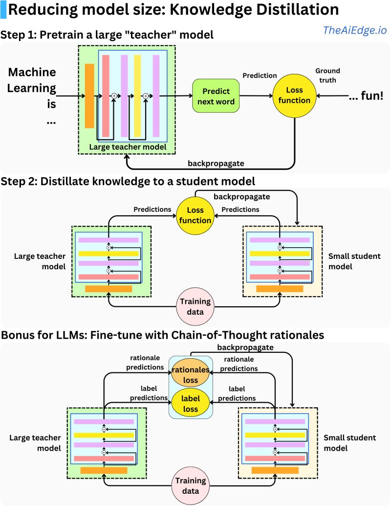
Mechanism
-
In standard supervised learning, models are trained to predict hard, one-hot labels. In contrast, knowledge distillation augments this with soft targets—probability distributions produced by the teacher. These targets encode relative likelihoods across all classes, providing richer supervisory signals.
-
The student is trained using a composite loss function that combines:
- Soft target loss: Kullback-Leibler (KL) divergence between the teacher’s and student’s softened output distributions.
- Hard target loss: Standard cross-entropy loss against ground-truth labels.
-
The loss function is:
-
where:
- \(L_{\text{hard}}\) is the cross-entropy loss with hard/true labels.
- \(L_{\text{soft}}\) is the KL divergence between the temperature-scaled softmax outputs:
- where \(T\) is the temperature parameter that controls the softness of the distribution. A higher \(T\) yields softer probabilities, revealing class similarities.
-
This dual-loss formulation helps the student generalize better by aligning both label fidelity and model semantics.
Types of Knowledge Distillation
Response-Based Distillation
- The most common and classical form.
- The student is trained to match the final output probabilities of the teacher model.
- Computationally simple and widely adopted.
- Used in frameworks like DistilBERT, TinyBERT, etc.
Feature-Based Distillation
- The student mimics internal hidden states or feature representations of the teacher.
- Often involves aligning intermediate activations across corresponding layers.
- Useful in vision tasks where spatial features are important.
- Examples include FitNets: Hints for Thin Deep Nets by Romero et al. (2015).
Relation-Based Distillation
- Focuses on matching relationships (e.g., distance, similarity, or angle) between samples in feature space across models.
- Encourages the student to learn the structural knowledge encoded in the teacher’s representation space.
- Often used in metric learning and ranking tasks.
- Example: Relational Knowledge Distillation by Park et al. (2019).
Distillation Modes
Offline Distillation
- The teacher is pre-trained and fixed.
- The student is trained using the frozen teacher’s outputs.
- This is the most common paradigm in industry.
Online Distillation
- Teacher and student are trained simultaneously.
- The teacher may itself be evolving (e.g., ensemble of students).
- Allows for dynamic refinement of knowledge but adds training complexity.
Self-Distillation
- The teacher and student share the same architecture.
- The teacher is typically an earlier version of the student (e.g., exponential moving average of weights).
- Demonstrated to improve performance even without model compression.
Why Use Knowledge Distillation Instead of Training Small Models from Scratch?
- Richer Supervision leading to Enhanced Generalization: The soft labels/targets from the teacher offer added supervisory signal by encoding subtle inter-class similarities (e.g., cat vs. tiger) and uncertainties that hard labels miss. This can guide the student to generalize better.
- Data Augmentation Effect: The additional information in soft labels effectively augments the supervision signal without needing more data.
- Performance Boost: Student models trained via distillation often outperform the same architecture trained directly on hard labels.
- Compression with Retention: Distillation enables substantial reduction in model size and latency, with minimal loss in accuracy.
- Regularization Effect: Soft labels (and the resulting dense supervision) lead to smoother gradients, which can act as a form of regularization, improving robustness.
- Data Efficiency: The student often requires fewer training epochs and can converge with less labeled data.
- Architecture Agnosticism: Students need not replicate the teacher’s structure, offering flexibility in design.
- Latency Reduction: Distilled students exhibit significant inference speedups, sometimes halving latency.
Why Knowledge Distillation Works
-
Soft targets: Soft targets offer weak but informative signals, guiding the student toward nuanced generalizations. Suppose a large teacher model is trained on CIFAR-100 and has convolutional filters that respond to features like pointy ears. When shown a Batman mask labeled “mask,” the model might still activate its cat filters slightly. This leads to a 0.1 probability for “cat.” Training the student on this soft distribution imparts a weak but useful signal that improves its understanding of cat features.
-
Ensemble effects: If an ensemble of models each captures different features—say, one detects pointy ears, another whiskers—distillation into a single student helps consolidate these distinct patterns, enhancing generalization.
-
Multiple views and theoretical foundations: Distillation behaves like weak supervision or multi-view learning. As explored in Towards Understanding Ensemble, Knowledge Distillation and Self-Distillation in Deep Learning by Allen-Zhu et al. (2023), distilled students can approximate ensemble behavior using soft targets.
Distillation in Practice
-
Knowledge distillation intersects with adversarial robustness, privacy preservation, and transfer learning.
-
Most widely used form is response-based distillation, but feature-based and relation-based variants are active research areas.
-
Implementation nuances—teacher-student architecture differences, scheduling, or layer alignment—often require trial and error.
-
In On the Efficacy of Knowledge Distillation, Cho and Hariharan (2019) found that large teacher models can hurt student performance if there’s a capacity mismatch. Bigger is not always better.
-
In Improved Knowledge Distillation via Teacher Assistant, Mirzadeh et al. (2019) emphasized that the gap in capacity between teacher and student should be moderate for best results.
-
Thus, a practical takeaway is to perform offline, response-based distillation using a slightly smaller student model for performance gains with minimal tuning.
-
Recent work such as Well-Read Students Learn Better by Turc et al. (2019) shows that Pre-trained Distillation (PD)—pretraining compact models before distillation—yields better results in NLP tasks. The recommended 3-step process is:
- Pre-train the compact model (student) on the same masked language modeling (MLM) objective used in BERT.
- Distill from a large, task-specific teacher model using response-based offline distillation. For example, if the downstream task is Natural Language Inference (NLI), use the teacher to produce logits for each class (entailment, contradiction, neutral), and minimize KL divergence with the student’s logits.
- Fine-tune the distilled student on the task-specific dataset, such as training on the CoNLL 2003 dataset for Named Entity Recognition (NER).
- This procedure has the advantage of being architecture-agnostic, making it practical for real-world deployment where the student architecture may differ substantially from the teacher.
-
Pretrained distilled models are now widely accessible. In NLP, libraries such as Hugging Face provide compact and distilled versions like DistilBERT and TinyBERT, often with task-specific checkpoints. In computer vision, Facebook’s d2go and DeiT offer mobile-ready image classification models that were distilled from larger vision transformers.
-
Practitioners should consider leveraging these pretrained distilled models when seeking lower latency or deployment efficiency, especially when retraining from scratch is resource-prohibitive.
Reverse Distillation
-
In reverse distillation, a small model acts as the teacher and a larger model is the student.
-
Particularly useful in noisy datasets (e.g., CTR prediction) where large models overfit easily.
-
In Investigating the Impact of Model Width and Density on Generalization in Presence of Label Noise, Xue et al. (2024) demonstrates this technique in high-label-noise regimes. Particularly, they show that using soft labels from a smaller model can regularize and stabilize large model training under label noise.
-
Process:
- Train a small, clean model on a curated subset.
- Use it to produce soft labels for the noisy data.
- Train the large model using these regularized targets.
Weak Supervision via Distillation
-
Distillation enables semi-supervised learning. Here’s the procedure:
- Train a high-capacity teacher on a small labeled set.
- Use it to label a larger unlabeled dataset.
- Train a compact student model on the combined data.
-
This approach has been successfully used in real-world settings such as Lessons from building acoustic models with a million hours of speech by Parthasarathi and Strom (2019), which trained acoustic models with over a million hours of speech data.
Compute vs. Memory Bottlenecks
-
The latency gains from deploying a distilled student model depend heavily on whether inference in your target environment is compute-bound or memory-bound.
-
Compute-bound workloads:
- For compute-bound workloads, where the runtime is dominated by arithmetic operations (FLOPs), such as large matrix multiplications, convolutions, activation functions, etc., knowledge distillation can yield substantial improvements here because a well-designed student typically has fewer parameters, fewer layers, and reduced hidden dimensions, directly lowering the FLOP count.
- These savings are realized as long as the hardware can execute the smaller architecture more efficiently without underutilizing compute units.
- However, on certain GPU architectures optimized for large, dense operations, very small models may not fully saturate the compute pipeline, leading to less-than-expected speedups.
-
Memory-bound workloads:
- For memory-bound workloads, where the runtime is not dominated by arithmetic, but by the cost of moving data (weights, activations) between memory and compute units, distillation can help if the student model’s parameter footprint is significantly smaller than the teacher’s, reducing weight fetches and intermediate activation storage.
- This is particularly valuable for deployment on edge devices or accelerators with limited memory bandwidth, where the teacher’s size would otherwise bottleneck inference.
- Gains are more pronounced if the smaller model fits entirely into faster memory tiers (e.g., GPU cache or on-chip SRAM), reducing costly DRAM accesses.
-
-
In practice, many real-world deployments see mixed bottlenecks, and the benefits of knowledge distillation are twofold:
- Lower FLOPs \(\rightarrow\) improved compute-bound performance.
- Smaller parameter and activation footprint \(\rightarrow\) improved memory-bound performance.
-
Importantly, unlike other model compression techniques such as quantization and pruning—which may keep much of the original model’s execution pattern—distillation produces a new, smaller dense architecture, making it easier for standard inference engines and hardware to exploit the reduction in both compute and memory requirements.
Limitations and Challenges
-
Capacity Gap: On the Efficacy of Knowledge Distillation by Cho and Hariharan (2019) demonstrates that extremely large teacher models can be poor mentors if the student’s capacity is too low—it cannot mimic the teacher effectively. Put simply, if the student model is too weak, distillation may degrade performance. Early stopping of the teacher may yield less “over‑fitted” soft labels that are more deliverable to the student.
-
Architecture Mismatch: Effectiveness can be reduced when the teacher and student architectures differ substantially.
-
Poor transfer on complex tasks: Results on datasets like ImageNet often trail behind simpler benchmarks unless carefully tuned.
-
Higher tuning cost: In contrast to quantization and pruning, distillation often requires more experimentation and task-specific adaptation.
Model Pruning
- Model pruning is a technique for compressing and accelerating deep neural networks by eliminating redundant parameters—either individual weights or structured components such as entire neurons, filters, or layers—without significantly degrading model performance. This compression facilitates faster inference, lower memory usage, and often improved generalization when carefully applied.
Formal Definition
-
Let \(f(x; \theta)\) be a trained neural network model parameterized by \(\theta \in \mathbb{R}^n\). Pruning aims to construct a sparsified parameter vector \(\theta' \in \mathbb{R}^n\) such that:
\[\theta'_i = \begin{cases} 0, & \text{if } i \in P \\ \theta_i, & \text{otherwise} \end{cases} \quad \text{where } P \subset \{1, \ldots, n\}\]- and the pruned model \(f(x; \theta')\) satisfies:
- where \(L\) denotes the loss function over the task of interest.
Rationale and Theoretical Motivation
- The core insight underpinning pruning is that modern deep networks are typically overparameterized. Empirical studies, such as Learning both Weights and Connections for Efficient Neural Networks by Han et al. (2015), demonstrate that up to 90% of weights in large-scale models can be pruned with negligible loss in accuracy. The underlying explanation aligns with the Lottery Ticket Hypothesis proposed in The Lottery Ticket Hypothesis: Finding Sparse, Trainable Neural Networks by Frankle & Carbin (2019), which posits that:
“A dense, randomly-initialized neural network contains a subnetwork that, when trained in isolation, can match the performance of the original network.”
- This hypothesis supports the idea that training a large model enables discovery of a performant sparse subnetwork, which can be extracted via pruning.
Types of Pruning
Unstructured Pruning
-
Unstructured pruning eliminates individual weights regardless of their position in the weight tensor. It is formally defined by selecting a mask \(M \in \{0, 1\}^n\) applied element-wise to the parameter vector \(\theta\), resulting in a sparse model:
\[\theta' = M \odot \theta\]-
where \(\odot\) denotes the Hadamard product. Criteria for zeroing elements commonly include:
- Magnitude-based pruning (e.g., remove smallest | weights |),
- Gradient-based importance metrics,
- Second-order methods (e.g., Hessian-based sensitivity).
-
-
Although unstructured pruning achieves high sparsity, it often provides limited inference acceleration on conventional hardware due to irregular memory access patterns.
Implementation:
- PyTorch:
torch.nn.utils.prunesupports various unstructured pruning strategies. -
TensorFlow:
tensorflow_model_optimization.sparsity.kerasallows weight pruning during training. - Example:
import torch.nn.utils.prune as prune
prune.l1_unstructured(module, name='weight', amount=0.8)
Structured Pruning
-
Structured pruning removes entire structural components of the model, such as:
- Filters in convolutional layers,
- Neurons in fully-connected layers,
- Heads in transformers,
- Layers or blocks in residual networks.
-
This results in a reduced model size and faster inference due to preservation of dense matrix formats.
-
Common importance metrics include:
- L1/L2 norm of filters, proposed in Han et al. (2015),
- Average activation magnitude,
- Taylor approximation of loss change,
- Shapley values.
-
Implementation:
Pruning Workflow
- A typical pruning pipeline consists of the following stages:
Step 1: Train the Full Model
- Train the original model to convergence using standard procedures.
Step 2: Apply Pruning Mask
-
Determine and apply pruning masks using one of the supported strategies. This can occur:
- Post-training: Prune after the model is fully trained.
- During training: Gradually prune weights over several epochs.
Step 3: Fine-Tune the Pruned Model
-
Retrain the pruned model to recover lost accuracy. The most effective method is learning rate rewinding, where:
- Training is resumed from an earlier weight checkpoint.
- The learning rate is reset to a higher value Comparing Rewinding and Fine-tuning in Neural Network Pruning by Renda et al. (2020).
-
Alternatively, weight rewinding may be used to reset weights of surviving parameters to their earlier values (e.g., 1/3 of training completed).
Compute vs. Memory Bottlenecks
-
Whether pruning improves inference latency depends strongly on the primary performance bottleneck of the workload:
Compute-bound workloads:
- For compute-bound workloads, where the runtime is dominated by arithmetic operations (FLOPs), such as large matrix multiplications, convolutions, activation functions, etc., reducing model size only helps if pruning directly lowers the number of executed operations and the hardware can exploit the new shape efficiently.
- For example, moderate structured pruning may still yield negligible gains on GPUs optimized for dense matrix multiplication unless the reduction crosses hardware-friendly dimensions that change kernel execution patterns (e.g., multiples of warp sizes or tensor core tile sizes).
- Unstructured pruning typically does not lower FLOP count in standard dense kernels, so compute-bound latency may remain unchanged.
Memory-bound workloads:
-
- For memory-bound workloads, where the runtime is not dominated by arithmetic, but by the cost of moving data (weights, activations) between memory and compute units, pruning can help by reducing the total parameter and activation footprint. This reduces the volume of data transferred and ultimately leads to fewer memory accesses and potentially higher throughput—especially when weights and activations no longer exceed cache capacities.
- This benefit is more pronounced in unstructured pruning or extreme structured pruning, where parameter reduction meaningfully shrinks memory traffic though this often requires specialized hardware/software support.
-
In summary, if the system is compute-bound, the time saved by transferring fewer parameters is negligible because the main delay is in processing operations, not in moving data. Moreover, unstructured pruning may not reduce computational cost on dense-optimized hardware without sparse acceleration kernels, meaning FLOP counts—and thus latency—stay similar. Structured pruning fares better but still depends heavily on whether the hardware kernels adapt efficiently to the new tensor shapes.
Practical Considerations
Target Sparsity
- Target sparsity (e.g., 80%) must be tuned experimentally. Aggressive sparsity often requires multiple pruning–fine-tuning cycles.
Compatibility
-
Pruning can be difficult for architectures with:
- Skip connections (e.g., ResNets),
- Attention modules with tight dimensional constraints.
-
Custom pruning logic may be required.
Deployment Readiness
- Sparse inference is not universally supported. Quantization-aware or hardware-specific pruning (e.g., \(N:M\) sparsity) may be necessary for real-world acceleration. As noted in What is the State of Neural Network Pruning? by Blalock et al. (2020), real benefits often depend on framework and hardware support.
Comparative Analysis
| Aspect | Unstructured Pruning | Structured Pruning |
|---|---|---|
| Targets | Individual weights | Filters, neurons, heads, layers |
| Benefits | Compression | Compression + inference acceleration |
| Implementation Ease | High | Moderate to low |
| Framework Support | TensorFlow, PyTorch | TorchPruner, Torch-Pruning |
| Inference Speedup | Limited | Significant |
Implementing Pruning in PyTorch and TensorFlow
- Modern deep learning frameworks provide built-in utilities to simplify pruning workflows. Below, we describe practical approaches in both PyTorch and TensorFlow.
PyTorch Pruning
-
PyTorch offers flexible pruning utilities via the
torch.nn.utils.prunemodule. This supports both unstructured and structured pruning. -
Unstructured Pruning Example (L1-based weight pruning):
import torch
import torch.nn.utils.prune as prune
import torch.nn as nn

model = nn.Sequential(
    nn.Linear(512, 256),
    nn.ReLU(),
    nn.Linear(256, 10)
)

# Prune 50% of weights in the first Linear layer
prune.l1_unstructured(model[0], name='weight', amount=0.5)

# To remove the pruning reparameterization and finalize pruning
prune.remove(model[0], 'weight')
- Structured Pruning Example (entire neuron/channel pruning):
# Prune 30% of channels (columns) in the second Linear layer
prune.ln_structured(model[2], name='weight', amount=0.3, n=2, dim=0)
prune.remove(model[2], 'weight')
-
PyTorch Pruning Resources:
- PyTorch pruning tutorial
- Torch-Pruning library – advanced dependency-aware structured pruning
- TorchPruner – structured pruning with visual feedback
TensorFlow Pruning
-
TensorFlow provides pruning support via the
tensorflow_model_optimizationtoolkit. It supports sparsity-aware training by gradually zeroing out weights. -
Basic Workflow:
import tensorflow as tf
import tensorflow_model_optimization as tfmot

prune_low_magnitude = tfmot.sparsity.keras.prune_low_magnitude

# Define prunable model
model = tf.keras.Sequential([
    prune_low_magnitude(tf.keras.layers.Dense(256, activation='relu'),
                        input_shape=(512,)),
    prune_low_magnitude(tf.keras.layers.Dense(10))
])

# Compile and train
model.compile(optimizer='adam', loss='sparse_categorical_crossentropy')
model.fit(x_train, y_train, epochs=5)

# Strip pruning wrappers before saving/export
model = tfmot.sparsity.keras.strip_pruning(model)
- Set Pruning Schedule:
pruning_schedule = tfmot.sparsity.keras.PolynomialDecay(
    initial_sparsity=0.0,
    final_sparsity=0.8,
    begin_step=0,
    end_step=1000
)
-
TensorFlow Pruning Resources:
- TensorFlow Model Optimization Guide
- Supports only unstructured pruning during training
- Can export TFLite-compatible sparse models for edge inference
Mixed Precision Training
Overview
-
Mixed precision is a technique used to speed up neural network training by utilizing both 16-bit and 32-bit floating-point types—primarily
float16,bfloat16, andfloat32. Traditionally, models rely on thefloat32dtype, which uses 32 bits of memory per value. However, many modern hardware accelerators are optimized to perform faster computations and memory access with 16-bit types. This means that usingfloat16orbfloat16, which only take 16 bits each, can lead to significant performance gains. -
The key insight behind mixed precision is that not all parts of a model require the full precision of
float32. For example, many operations can be safely executed usingfloat16orbfloat16without compromising the final evaluation metrics such as accuracy. This is where Automatic Mixed Precision (AMP) comes in—it automatically determines the most appropriate precision for each operation, balancing performance with numerical stability.- The term “numeric stability” refers to how much using lower precision (like
float16) affects a model’s quality. If certain operations are sensitive to precision loss, AMP keeps them infloat32to preserve model accuracy. By assigning the appropriate dtype to each operation, mixed precision reduces the model’s runtime and memory footprint while maintaining comparable performance.
- The term “numeric stability” refers to how much using lower precision (like
-
In summary, mixed precision combines the efficiency of 16-bit operations with the robustness of 32-bit computations to optimize deep learning training workflows.
How Mixed Precision Training Works
-
Mixed precision training is a performance optimization technique that accelerates neural network training by leveraging lower-precision arithmetic—primarily half-precision floating-point (
float16)—without compromising model accuracy or convergence stability. -
At its core, the concept is straightforward: replacing standard single-precision (
float32) operations with half-precision (float16) can roughly halve memory usage and significantly reduce training time. However, implementing this substitution safely and effectively is non-trivial due to the numerical limitations of lower-precision formats. -
By combining dual weight representations, selective precision, and dynamic loss scaling, mixed precision training enables significant reductions in training time and memory consumption—often with negligible impact on model accuracy. As demonstrated in Mixed Precision Training by Narang et al. (2018), these methods allow a wide range of models to train to convergence reliably and efficiently using
float16computations. -
Challenges with Half Precision:
-
Lower-precision formats like
float16have a reduced dynamic range and lower numerical precision compared tofloat32. One critical issue is underflow, where extremely small gradient values become indistinguishable from zero due to rounding errors inherent in the limited precision. This is especially problematic during backpropagation, as many gradient updates are naturally very small but still essential for accurate model convergence. If too many of these values are rounded to zero or becomeNaN(Not a Number), the model may fail to learn altogether. -
The following figure from the Mixed Precision Training paper illustrates a key finding that naïvely switching to
float16causes any gradient smaller than \(2^{-24}\) to be “swallowed”—effectively zeroed out. In their experiments, this resulted in approximately 5% of all gradient updates being discarded, severely impeding the training process:
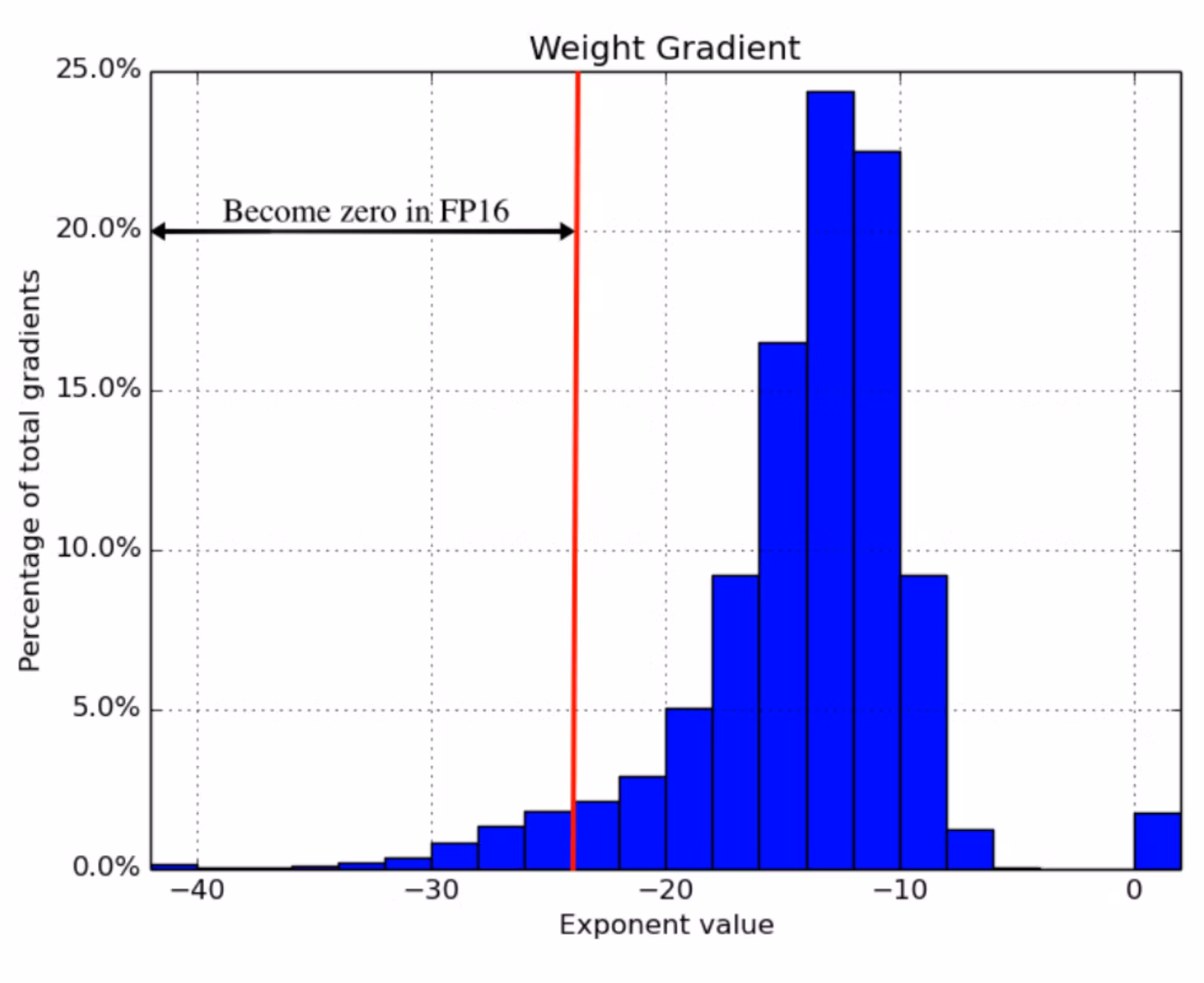
-
-
Techniques for Safe Mixed Precision Training:
-
To mitigate these numerical instabilities, the authors propose a systematic approach combining three key strategies. When used together, these allow safe and effective training with
float16precision:- Maintaining Dual Weight Copies (Master Weights Strategy)
- Each model weight is stored in two formats: a full-precision (
float32) “master copy” and a lower-precision (float16) copy. During forward and backward passes, computations are performed using thefloat16version to benefit from faster execution and lower memory usage. However, the actual weight updates are applied to thefloat32master weights using gradients computed infloat16but cast tofloat32. This preserves update accuracy and avoids the accumulation of precision errors during training.
- Each model weight is stored in two formats: a full-precision (
- Selective Precision Application (Mixed-Dtype Execution)
- Not all neural network operations are equally sensitive to reduced precision. Many element-wise operations (e.g., activation functions or layer normalization) are safe to compute in
float16, while others—such as softmax, batch normalization, and gradient accumulation—requirefloat32to maintain stability. Mixed precision training selectively appliesfloat16where safe and retainsfloat32where necessary. This fine-grained control over data types allows the model to reap performance benefits without sacrificing numerical stability/reliability.
- Not all neural network operations are equally sensitive to reduced precision. Many element-wise operations (e.g., activation functions or layer normalization) are safe to compute in
- Loss Scaling
- To address the underflow problem, the loss value is multiplied by a scalar factor (commonly 8, 16, or 128) before backpropagation. This process, known as loss scaling, proportionally increases all gradient values, elevating small gradients above the
float16precision threshold of \(2^{-24}\). After gradients are computed, the scaling factor is removed (by division) before the optimizer applies the updates. - Care must be taken to avoid overflow, which occurs when values exceed the representable range of
float16, leading toInforNaNvalues. Adaptive loss scaling strategies—where the scaling factor is dynamically adjusted based on gradient statistics—are often employed to balance between underflow and overflow.
- To address the underflow problem, the loss value is multiplied by a scalar factor (commonly 8, 16, or 128) before backpropagation. This process, known as loss scaling, proportionally increases all gradient values, elevating small gradients above the
- Maintaining Dual Weight Copies (Master Weights Strategy)
-
How PyTorch Automatic Mixed Precision Works
-
With a solid understanding of mixed precision training established, we can now explore how PyTorch streamlines this powerful optimization technique through its Automatic Mixed Precision (AMP) API. While mixed precision training has long been theoretically feasible—typically requiring manual tensor casting to
float16and careful loss scaling—PyTorch removes much of this complexity. Its AMP API makes the process highly accessible, offering a streamlined, production-ready solution that demands only minimal code modifications. -
PyTorch’s AMP achieves this by abstracting the underlying mechanics through two key components:
autocastandGradScaler.autocastenables selective precision execution, automatically determining which operations benefit from half-precision without sacrificing accuracy. Simultaneously,GradScalermanages dynamic loss scaling, helping to prevent issues like gradient underflow and ensuring stable convergence. This integration offers developers substantial speedups—often reducing training times by 50–60%—and improves memory efficiency, all without compromising model stability or performance. -
This practical implementation is a direct evolution of the concepts outlined in the Mixed Precision Training research paper. AMP embodies how advanced techniques from cutting-edge research can be distilled into user-friendly tools that enhance real-world machine learning workflows.
-
Prior to AMP, implementing mixed precision was a labor-intensive process. Developers had to manually cast tensors, implement and tune custom loss scalers, and safeguard against the risks of instability. The introduction of PyTorch’s
torch.cuda.ampmodule represents a major leap forward, encapsulating best practices and democratizing access to high-performance training. -
AMP is especially effective on modern NVIDIA GPUs—such as those based on Volta, Turing, Ampere, or newer architectures—which include specialized Tensor Cores designed for half-precision operations. However, even on older or unsupported hardware, users may still see performance benefits due to more efficient memory usage and reduced data movement.
-
In summary, PyTorch’s AMP bridges the gap between theoretical efficiency and practical deployment, making state-of-the-art training techniques both accessible and impactful across a wide range of hardware and use cases.
Overview of AMP Components
-
PyTorch’s AMP functionality is implemented via the
torch.cuda.ampmodule and relies on two key primitives:-
torch.cuda.amp.autocast: A context manager that automatically casts operations to the appropriate precision (float16orfloat32) based on operation type and hardware support. This enables a seamless mix of half-precision and full-precision computations without explicit manual intervention. -
torch.cuda.amp.GradScaler: A utility that handles dynamic loss scaling. It scales the loss to prevent underflow in gradient computations and then unscales it before applying the optimizer step. The scaler also detects and skips optimizer steps with invalid gradients (e.g.,NaNorInf), adjusting the scale factor dynamically to maintain numerical stability.
-
Practical Implementation in a Training Loop
- The following example demonstrates how mixed precision training is incorporated into a standard PyTorch training loop. Lines marked with
# NEWindicate additions or modifications required to enable AMP.
self.train()
X = torch.tensor(X, dtype=torch.float32)
y = torch.tensor(y, dtype=torch.float32)

optimizer = torch.optim.Adam(self.parameters(), lr=self.max_lr)
scheduler = torch.optim.lr_scheduler.OneCycleLR(
    optimizer, self.max_lr,
    cycle_momentum=False,
    epochs=self.n_epochs,
    steps_per_epoch=int(np.ceil(len(X) / self.batch_size)),
)
batches = torch.utils.data.DataLoader(
    torch.utils.data.TensorDataset(X, y),
    batch_size=self.batch_size, shuffle=True
)

# NEW: Initialize GradScaler for dynamic loss scaling
scaler = torch.cuda.amp.GradScaler()

for epoch in range(self.n_epochs):
    for i, (X_batch, y_batch) in enumerate(batches):
        X_batch = X_batch.cuda()
        y_batch = y_batch.cuda()
        optimizer.zero_grad()

        # NEW: Forward pass with autocast for mixed precision
        with torch.cuda.amp.autocast():
            y_pred = model(X_batch).squeeze()
            loss = self.loss_fn(y_pred, y_batch)

        # NEW: Scale loss and perform backward pass
        scaler.scale(loss).backward()

        lv = loss.detach().cpu().numpy()
        if i % 100 == 0:
            print(f"Epoch {epoch + 1}/{self.n_epochs}; Batch {i}; Loss {lv}")

        # NEW: Unscale gradients, perform optimizer step, update scaler
        scaler.step(optimizer)
        scaler.update()

        scheduler.step()
-
Implementation Notes and Best Practices:
-
Device compatibility: AMP is optimized for NVIDIA GPUs with Tensor Cores, particularly those with compute capability ≥ 7.0 (Volta architecture or newer). While it will run on other hardware, performance gains may vary.
-
Model compatibility: Most standard PyTorch layers (e.g.,
nn.Linear,nn.Conv2d,nn.ReLU) are AMP-compatible. However, custom operations or third-party libraries may require manual inspection to ensure compatibility or appropriate casting. -
Gradient stability: The
GradScalerperforms automatic gradient anomaly detection, skipping optimizer steps when gradients containInforNaNvalues. This safeguards training from diverging due to numerical instability. -
Loss scaling strategy: The
GradScaleruses dynamic loss scaling by default, which adjusts the scaling factor at runtime based on gradient statistics. This is typically preferred over static scaling for its adaptive robustness.
-
Loss and Gradient Scaling with GradScaler
-
A fundamental challenge of half-precision (
float16) training is the limited dynamic range, which can cause small-magnitude gradients to underflow—i.e., round down to zero—during backpropagation. This occurs because when an operation receivesfloat16inputs in the forward pass, the resulting gradients computed in the backward pass are also infloat16, unless explicitly handled. In deep learning, many gradients—particularly in early layers or at later training stages—can be extremely small, and when these are flushed to zero, their corresponding weight updates are effectively lost, impeding learning. -
To mitigate this, PyTorch introduces loss scaling, a technique that amplifies loss values and their corresponding gradients during the backward pass to avoid underflow. The process works as follows:
- The loss is multiplied by a scale factor before backpropagation.
- Gradients are computed on this scaled loss, resulting in proportionally larger values.
- These gradients are then unscaled before the optimizer applies the update, preserving the intended learning dynamics.
-
This technique is implemented via the
torch.cuda.amp.GradScalerobject, which automates both the scaling and unscaling process, as well as overflow detection and recovery. The goal is to find a balance: a scale factor high enough to preserve small gradients, yet not so high that large gradients overflow and becomeinf—maintaining a balance between underflow and overflow.
Dynamic Scaling with Exponential Backoff
-
There is no single static loss multiplier that suits all models or all stages of training. Gradient magnitudes are typically much larger at the beginning of training and diminish as convergence nears. Rather than asking users to manually tune this value, PyTorch uses an adaptive approach based on exponential backoff.
-
The
GradScalerbegins with an initial scale (default: 65,536 or \(2^{16}\)) and periodically doubles it to maximize numerical range. If an overflow is detected—i.e., any gradient becomesinforNaN—the current update step is skipped, the scale is halved, and a cooldown counter is reset. This approach allows PyTorch to adaptively find a safe and efficient scaling factor over time, much like TCP congestion control adapts network throughput. -
This behavior can be configured via the
GradScalerconstructor:torch.cuda.amp.GradScaler( init_scale=65536.0, growth_factor=2.0, backoff_factor=0.5, growth_interval=2000, enabled=True )init_scale: The initial scaling factor.growth_factor: Multiplicative increase rate when no overflows are detected.backoff_factor: Reduction factor when an overflow is detected.growth_interval: Number of successful steps before scale growth is attempted.enabled: Whether AMP and scaling are active.
-
Operational Considerations:
-
GradScalermodifies key parts of the training loop:loss.backward()becomesscaler.scale(loss).backward()optimizer.step()becomesscaler.step(optimizer)- The call to
scaler.update()checks for overflows and adjusts the scale as needed.
-
It is important to note that overflows (
inf) are detectable and trigger corrective behavior. Underflows, however, are silent because zero gradients are not always erroneous. Thus, choosing a very low initial scale or a very long growth interval may cause the network to silently underperform or diverge. PyTorch’s large defaultinit_scalemitigates this risk. -
Internally, before the optimizer updates the model weights, the gradients (
.grad) are unscaled to ensure the learning rate and optimizer dynamics remain consistent with those expected infloat32training.
-
-
Checkpointing with GradScaler:
- Because
GradScaleris a stateful object that adapts over time, it must be saved and restored along with the model and optimizer during checkpointing. PyTorch provides simple APIs for this:
# Saving torch.save({ 'model_state_dict': model.state_dict(), 'optimizer_state_dict': optimizer.state_dict(), 'scaler_state_dict': scaler.state_dict() }, 'checkpoint.pt') # Loading checkpoint = torch.load('checkpoint.pt') model.load_state_dict(checkpoint['model_state_dict']) optimizer.load_state_dict(checkpoint['optimizer_state_dict']) scaler.load_state_dict(checkpoint['scaler_state_dict'])- By integrating
GradScalerinto the training process, PyTorch ensures that the numerical precision limitations offloat16do not compromise convergence, while still allowing significant performance and memory efficiency gains.
- Because
Automatic Precision Casting with the autocast Context Manager
-
The second key component of PyTorch’s AMP system is the
torch.cuda.amp.autocastcontext manager. WhileGradScaleraddresses numerical stability during backpropagation via loss scaling,autocastis responsible for precision control during the forward pass. -
Mixed precision training derives its speed and memory benefits primarily by executing selected operations in
float16rather thanfloat32. However, not all operations are equally safe or efficient in half precision. Some are numerically stable and performant when cast tofloat16, while others require higher precision to avoid instability or incorrect outputs. -
The
autocastcontext manager dynamically casts operations to the most appropriate precision at runtime. This casting is done based on an internal whitelist/blacklist system defined by PyTorch, taking into account both the operation type and the tensor data types involved. This enables users to delegate dtype management to PyTorch, avoiding manual casting and type-checking logic. -
How
autocastWorks Internally:- Operations such as matrix multiplications (
matmul), convolutions (conv2d), and other linear algebraic operations are generally safe to perform infloat16, and thus are automatically downcast when inside anautocastcontext. -
Conversely, operations that are sensitive to numerical precision—such as logarithms, exponentials, trigonometric functions, and large summations—are retained in
float32to ensure computational accuracy. - The following visuals (source), summarize these distinctions. The image below outlines common operations that benefit from
float16execution. These include core building blocks of deep learning models like matrix multiplications, dot products, and convolutions. Their stability in half precision makes them ideal candidates for mixed precision acceleration.
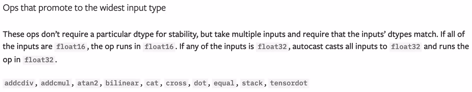
- In contrast, as shown in the image below (source), operations involving logarithms, exponentials, or statistical reductions tend to suffer from rounding errors in
float16and are therefore retained infloat32.
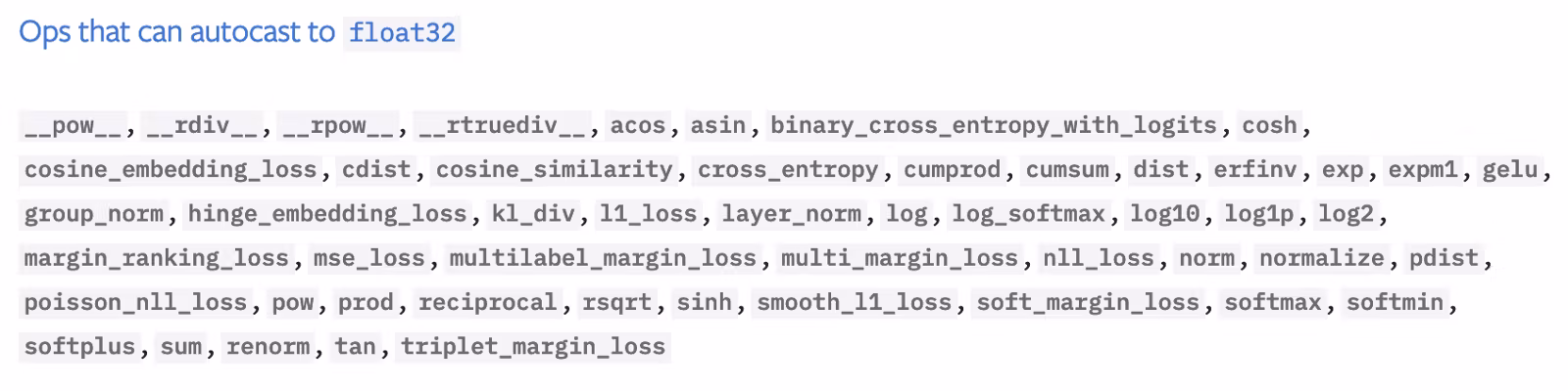
- Operations such as matrix multiplications (
-
Implications for Model Layers:
-
These rules imply that:
- Most layers (e.g., linear, convolutional, attention) benefit substantially from autocasting, due to their reliance on matrix operations.
- Most activation functions and normalization layers are less safe in
float16, and autocast will retain full precision where necessary. - The greatest performance gains are likely in deep CNNs or transformer models with many linear operations and matrix multiplications.
-
-
Using
autocastin Practice:- Enabling autocasting is simple and requires wrapping the forward pass in a context manager:
with torch.cuda.amp.autocast(): y_pred = model(X_batch).squeeze() loss = self.loss_fn(y_pred, y_batch)- All operations within the
autocast()context will be executed with optimal mixed precision, determined internally by PyTorch. Importantly, this casting behavior extends to the backward pass automatically—there is no need to wraploss.backward().
-
Best Practices and Notes:
- Autocast respects and supports a wide range of PyTorch operators out-of-the-box. Unless using custom operations or extensions, most models will run correctly without additional intervention.
- In-place operations (e.g.,
.add_()or.relu_()) can interfere with autocast’s internal precision control. Avoid in-place modifications insideautocast()blocks unless explicitly supported. - Autocast is deterministic and composable. It can be used inside model layers, training loops, or custom modules with consistent behavior.
- For inference scenarios, autocasting is also beneficial and can be enabled in evaluation mode to reduce memory usage without requiring
GradScaler.
Using AMP with Multiple GPUs
-
PyTorch’s Automatic Mixed Precision (AMP) functionality is fully compatible with multi-GPU training, enabling developers to scale up performance without sacrificing the benefits of mixed precision. Both of PyTorch’s multi-GPU parallelization strategies—
DistributedDataParallel(DDP) andDataParallel—support autocasting and gradient scaling, with minimal adjustments. -
AMP’s multi-GPU support is robust and integrates seamlessly into distributed training workflows. With only minor adjustments, developers can leverage both horizontal scaling and mixed precision optimization, achieving faster training with efficient GPU utilization across multiple devices.
-
DistributedDataParallel (DDP): AMP works out-of-the-box with DDP, which is the recommended strategy for multi-GPU training. The key requirement is to use one process per GPU, following the standard setup for DDP. This ensures independent autocast and
GradScalerinstances per GPU, maintaining stability and efficiency. -
DataParallel: AMP also works with
DataParallel, but with a caveat. SinceDataParalleluses a single process to drive multiple devices, it shares the autocast and scaling logic across GPUs. To accommodate this, one small adjustment must be made as outlined in the official AMP Examples guide. Specifically, ensure that loss scaling is only performed on the output of the model’s.forward()call on the main device, before broadcasting gradients. -
Implementation Tips:
- Refer to the Working with Multiple GPUs section in the PyTorch AMP documentation for detailed examples and best practices.
- Be mindful of numerical stability when using binary classification loss functions. The AMP documentation recommends preferring binary cross entropy with logits over binary cross entropy, as the logits version is more numerically stable and better suited for mixed precision.
-
Memory Considerations
-
One of the advertised benefits of mixed precision training, in addition to performance speedups, is reduced GPU memory consumption. As discussed in the earlier section on How Mixed Precision Works,
float16tensors require half the storage space of theirfloat32counterparts. This reduction in memory footprint can be particularly advantageous in training large-scale models, where memory constraints often limit batch size or model complexity. -
Although GPU compute is generally the primary bottleneck in training workloads, optimizing memory usage remains important. Efficient memory utilization enables:
- Larger batch sizes, which can improve training stability and convergence.
- The ability to fit deeper or wider models within available hardware constraints.
- Reduced reliance on gradient checkpointing or memory-efficient architectures.
-
PyTorch manages GPU memory allocation proactively. At the start of training, it reserves a block of GPU memory that it maintains throughout the training lifecycle. This behavior helps avoid runtime memory fragmentation and preempts crashes caused by other processes occupying memory mid-training. However, it also means that the effect of mixed precision on memory usage may not always be visible in a straightforward manner.
-
The figure below illustrates PyTorch’s memory reservation behavior with and without AMP enabled:
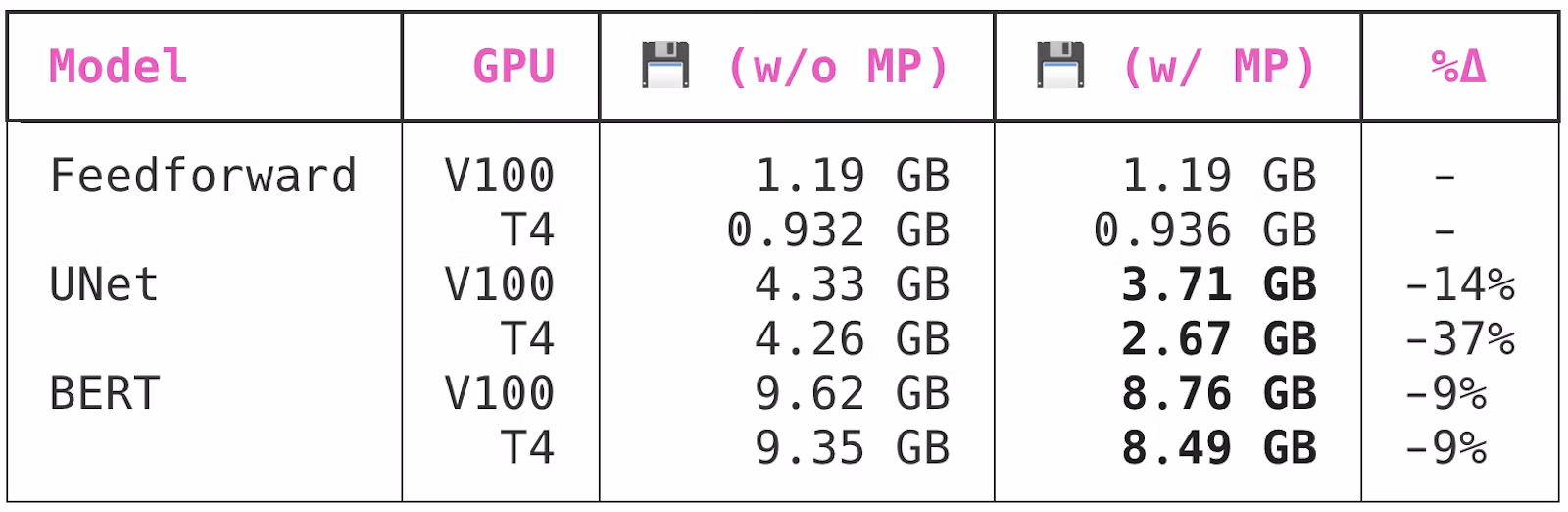
-
Interestingly, while both UNet and BERT models exhibit a reduction in memory usage when AMP is enabled, the gains are model-dependent. UNet, in particular, benefits significantly more than BERT. This discrepancy may result from differences in internal layer composition, memory allocation patterns, or the proportion of operations compatible with
float16. PyTorch’s memory allocator is largely opaque, making it difficult to pinpoint exact causes without in-depth profiling. -
Nonetheless, practitioners can generally expect mixed precision to reduce overall memory usage, especially in convolution-heavy models like UNet. This makes AMP not only a tool for acceleration but also a practical memory optimization strategy, particularly beneficial for users working within the limits of consumer-grade GPUs or training on multiple models in parallel.
Further Reading
-
For further reading and in-depth examples, consult the official documentation:
How TensorFlow Automatic Mixed Precision Works
-
Mixed precision training in TensorFlow is designed to accelerate deep learning workloads by leveraging the efficiency of lower-precision (
float16) arithmetic on supported hardware. With automatic mixed precision (AMP), TensorFlow streamlines the use of mixed-precision computation while preserving numerical stability and minimizing manual intervention. -
TensorFlow’s AMP support offers a robust, efficient, and production-ready pathway to accelerate model training with minimal code changes, using a hybrid approach similar to PyTorch. Operations are executed in
float16where safe for performance and memory efficiency, while numerically sensitive computations remain infloat32to preserve stability and ensure convergence. -
Built around the
mixed_precisionmodule, TensorFlow provides a high-level, intuitive interface for enabling efficient mixed-precision training. By leveraging global policies and loss scaling under the hood, TensorFlow abstracts away much of the complexity involved in training withfloat16. No manual casting or scaling logic is needed for most models, making integration straightforward for both experimentation and production. These features bring the practical benefits of faster computation and reduced memory usage—especially when training on modern GPUs—while maintaining the reliability of full-precision training. For a complete guide and reference examples, refer to the official TensorFlow mixed precision guide.
Conceptual Overview
-
Mixed precision training in TensorFlow works by executing computations in half-precision (
float16) where safe, and in single-precision (float32) where required for numerical stability. This selective usage of data types reduces memory bandwidth and speeds up computation, particularly on GPUs equipped with NVIDIA Tensor Cores (e.g., V100, T4, A100). These architectures are specifically designed to handle mixed-precision workloads efficiently. -
The two core features of TensorFlow’s AMP system are:
-
Global Policy Management: Mixed precision is enabled by setting a global or per-layer dtype policy to
'mixed_float16'. This instructs TensorFlow to automatically cast eligible operations tofloat16while retaining critical variables (e.g., weights, certain accumulators) infloat32. -
Loss Scaling with
LossScaleOptimizer: To mitigate the risk of underflow—when gradient values fall below the representable range offloat16—TensorFlow introduces automatic loss scaling. This mechanism adaptively maintains numerical stability without manual tuning, multiplying the loss by a scalar factor before backpropagation and reverting it afterward. This is enabled by wrapping a base optimizer withtf.keras.mixed_precision.LossScaleOptimizer.
-
-
These two features make mixed precision safe for most real-world training scenarios, enabling users to benefit from performance gains without manual tensor casting or custom scaling logic.
Practical Implementation in a Training Pipeline
- TensorFlow’s mixed precision training is designed to be seamless, requiring only a few lines of code to enable. The following example demonstrates a typical setup using the
tf.kerasAPI.
import tensorflow as tf
from tensorflow.keras import mixed_precision

# Enable mixed precision globally
mixed_precision.set_global_policy('mixed_float16')

# Define a model (example: simple MLP)
model = tf.keras.Sequential([
    tf.keras.layers.Dense(256, activation='relu'),
    tf.keras.layers.Dense(128, activation='relu'),
    tf.keras.layers.Dense(1)
])

# Wrap the optimizer with LossScaleOptimizer for stability
base_optimizer = tf.keras.optimizers.Adam(learning_rate=1e-3)
optimizer = mixed_precision.LossScaleOptimizer(base_optimizer)

# Compile the model
model.compile(optimizer=optimizer, loss='mse', metrics=['mae'])

# Prepare training data
X_train = tf.random.normal((10000, 20))
y_train = tf.random.normal((10000, 1))

# Train the model
model.fit(X_train, y_train, batch_size=64, epochs=10)
-
Explanation of Key Components:
-
set_global_policy('mixed_float16'): This sets the default computation policy across all layers to usefloat16where safe, while storing variables such as model weights infloat32to ensure stability. -
LossScaleOptimizer: The base optimizer (e.g.,Adam) is wrapped to apply dynamic loss scaling. This prevents numerical underflows by adapting the loss scaling factor based on gradient stability during training. -
Hardware Requirements: While AMP can be enabled on any GPU, maximum performance benefits are realized on NVIDIA GPUs with Tensor Cores, such as the Volta (V100), Turing (T4), or Ampere (A100) architectures.
-
-
Layer Compatibility and Custom Layers
-
Most built-in TensorFlow and Keras layers support AMP without modification. If you’re using custom layers or third-party code, ensure that:
- Operations numerically sensitive to precision are forced to
float32if needed (usingtf.cast). - Custom gradients are correctly handled, especially in layers using
tf.custom_gradient.
- Operations numerically sensitive to precision are forced to
-
-
Model Behavior and Performance Considerations:
-
Storage Format: Weights are stored in
float32internally, but computations are cast tofloat16where safe. This ensures a balance between performance and accuracy. -
Layer Compatibility: Most built-in Keras layers are fully compatible with AMP. Custom layers or third-party operations may require manual casting using
tf.cast()or explicit dtype management. -
Inference: After training, models trained with AMP can be saved and exported as usual. During inference, the
mixed_float16policy can remain active to reduce latency and memory usage, particularly for large batch sizes.
-
-
Best Practices for TensorFlow AMP:
- Enable AMP by default (i.e., use
mixed_float16) when training on Tensor Core GPUs, especially for models with substantial compute demands. Use dynamic loss scaling (enabled by default withLossScaleOptimizer) to maintain stability during training without the need for manual tuning. - Monitor training for gradient anomalies (e.g., sudden spikes in loss). Although AMP is robust, occasional divergence may indicate the need for a lower initial loss scale or a refined model architecture.
- Use benchmark tools (e.g., TensorBoard, NVIDIA Nsight Systems) to validate performance gains and ensure your training benefits from mixed precision on supported hardware.
- Enable AMP by default (i.e., use
Performance Benchmarks
- To evaluate the real-world impact of mixed precision training, consider benchmarks run across three distinct neural network architectures using TensorFlow’s AMP implementation.
- These benchmarks demonstrate that automatic mixed precision should be one of the first performance optimizations you apply to your TensorFlow training scripts. In large-scale models, AMP can lead to dramatic reductions in training time—up to 60%—with minimal code changes (typically under 5 lines). Especially when training on modern GPU architectures, the performance uplift can be essential to reducing costs and iteration times in production-scale machine learning.
-
The experiments were conducted on AWS EC2 instances using both last-generation and current-generation NVIDIA GPUs.
- Hardware setup:
- V100 (Volta architecture) via
p3.2xlarge - T4 (Turing architecture) via
g4dn.xlarge
- V100 (Volta architecture) via
-
Framework: Recent TensorFlow builds with CUDA 10.0, orchestrated using the Spell API
-
Models Tested:
-
Feedforward Network A fully connected feedforward network trained on tabular data from the Rossmann Store Sales Kaggle competition. Codebase: GitHub repository
-
UNet A medium-sized convolutional model used for image segmentation on the Segmented Bob Ross Images dataset. Codebase: GitHub repository
-
BERT A large-scale transformer model (
bert-base-uncased) trained on the Tweet Sentiment Extraction dataset using Hugging Face’s Transformers. Codebase: GitHub repository
-
- Benchmark Results:
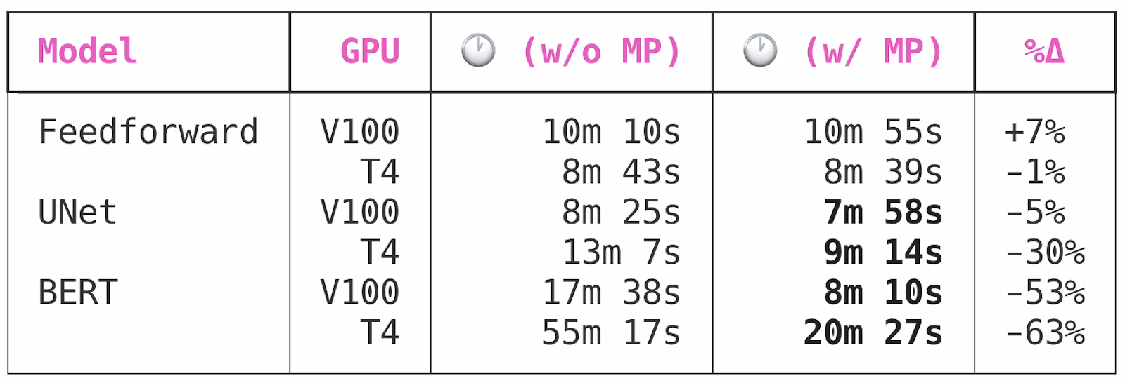
-
Observations:
-
Feedforward Network: Being a small model with minimal computational complexity, this architecture saw negligible benefit from mixed precision training. The data throughput and model size are simply too limited to leverage Tensor Core acceleration.
-
UNet (Medium-Scale Model): With approximately 7.7 million parameters, UNet showed meaningful improvements in training time. The impact of AMP varied by hardware:
- V100: ~5% training time reduction
- T4: ~30% reduction This disparity highlights how more recent GPU architectures (like Turing) extract greater benefit from Tensor Core utilization.
-
BERT (Large-Scale Model): Mixed precision provided transformational benefits for BERT:
- Training time reduced by 50–60% on both GPU types
- No degradation in training loss or final model performance This demonstrates that AMP is especially advantageous for large transformer-based models where computational demand is high.
-
Key Takeaways
-
TensorFlow’s automatic mixed precision (AMP) support offers a robust, efficient, and production-ready pathway to accelerate model training with minimal code changes. By executing safe operations in
float16while preserving critical numerical precision withfloat32where needed, TensorFlow achieves an optimal balance of performance and stability. -
Ease of Integration: Mixed precision can be enabled in just a few lines using
mixed_precision.set_global_policy('mixed_float16')and wrapping the optimizer withLossScaleOptimizer. No manual casting or scaling logic is needed for most models. -
Hardware Acceleration: Significant speedups are realized on NVIDIA GPUs with Tensor Cores (e.g., V100, T4, A100). These architectures are specifically designed to handle mixed-precision workloads efficiently.
-
Scalability: The performance benefits of AMP scale with model size. While small models may see limited gains, medium-to-large models—particularly convolutional networks and transformers—can experience training time reductions of 30–60% or more.
-
Numerical Stability: Automatic loss scaling ensures that mixed precision does not compromise training convergence. Gradient underflows are mitigated adaptively, making AMP safe for most real-world training scenarios.
Recommendations
- Enable AMP by default when training on Tensor Core GPUs, especially for models with substantial compute demands.
- Benchmark performance for your specific model and dataset, as the impact of mixed precision can vary depending on architecture, data pipeline, and hardware.
- Use dynamic loss scaling (enabled by default with
LossScaleOptimizer) to maintain stability without the need for manual tuning.
Low-Rank Decomposition & Adaptation
Overview
-
Large language models (LLMs) and deep neural networks often rely on massive weight matrices that are expensive to store and compute. However, in many cases, these matrices exhibit redundancy—meaning they can be approximated by lower-rank structures without significantly compromising the model’s predictive performance. Low-rank decomposition exploits this insight by factorizing large matrices into the product of two smaller matrices.
-
The motivation is twofold:
- Efficiency: Reducing the number of parameters and operations accelerates training and inference.
- Compression: Enables model deployment on memory-constrained devices by lowering storage requirements.
-
This technique is especially attractive when used with techniques like quantization, pruning, or transfer learning, as it complements them without requiring extensive retraining.
Formal Definition
-
The core idea: replace a large dense weight matrix
\[W \in \mathbb{R}^{d \times d}\]- with two smaller matrices:
- where \(r \ll d\). The original weight matrix is then approximated as:
-
This reduces the parameter count from \(O(d^2)\) to \(O(rd)\), which is a significant gain when \(r \ll d\). During inference or training, instead of computing:
\[y = Wx\]- we compute:
-
This allows models to retain much of their representational power while becoming faster and more compact.
Concept
-
Freeze original pretrained weights; add trainable adapters \(A, B\) for each dense layer such that:
- Efficiency: Only train few parameters (e.g. \(2dr\) per layer). For large LLMs, can reduce fine-tuning parameters by \(10^3 – 10^{4×}\) while achieving competitive results.
- Popular in federated settings (see above).
Low-Rank Correction for Quantization
-
Counteract quantization-induced error in activation domains. We approximate the full-precision weight matrix:
\[W \in \mathbb{R}^{d \times d}\]- as the product of two low-rank matrices:
-
This reduces the parameter count from \(O(d^2)\) to \(O(rd)\), significantly lowering storage and compute cost.
-
In quantization-aware settings, this is often extended to:
-
where:
- \(Q\) is the quantized version of \(W\), e.g.,
int4orint8 - \(A B\) is a low-rank full-precision correction term on unquantized activations
- \[A \in \mathbb{R}^{d \times r}, B \in \mathbb{R}^{r \times d}\]
- \(Q\) is the quantized version of \(W\), e.g.,
-
This hybrid scheme (quantized base + low-rank residual) allows retaining much of the accuracy of full-precision models while gaining the memory and speed benefits of quantization.
- Solve via joint optimization: alternating minimization to fit both quantized and low-rank components to minimize output reconstruction error. With ranks at 10% of weight size, activation error gaps can be halved; with 30% rank, closed completely.
- Fits well with post-training quantization pipelines. Works across calibration sets without full retraining.
Quantized Low-Rank Adaptation Techniques
- Low-Rank Adaptation (LoRA) techniques allow efficient fine-tuning of large-scale pre-trained models by updating only a small number of additional low-rank matrices while freezing the original weights. Several recent advancements extend this idea by incorporating quantization, yielding memory-efficient and compute-friendly training pipelines. Below, we explore three major variants: LQ-LoRA, QLoRA, and QA-LoRA.
LQ‑LoRA: Quantized + Low-Rank Adaptation
- LQ-LoRA was introduced in Guo et al., 2023 as a memory-efficient fine-tuning approach that combines low-bit quantization with learnable low-rank adapters.
Overview
- Each full-precision weight matrix \(W \in \mathbb{R}^{d \times d}\) is decomposed into:
- \(Q \in \mathbb{R}^{d \times d}\): a low-bit quantized matrix (e.g., 2.75 bits), kept frozen
- \(A \in \mathbb{R}^{d \times r}\), \(B \in \mathbb{R}^{r \times d}\): low-rank full-precision matrices, learnable
Key Properties
- The quantized base matrix \(Q\) captures the main representational power of the original model, without requiring updates during fine-tuning.
- The low-rank matrices \(A\) and \(B\) adapt the model to the downstream task.
- Enables sub-3-bit quantization without major degradation in task performance.
- Requires only ~27 GB of GPU memory to fine-tune a Llama 2 70B model, enabling large model training on commodity hardware.
Pros
- High compression without sacrificing much accuracy.
- Applicable to ultra-large models (e.g., Llama 2 70B).
- Training only the LoRA adapters ensures stability even at low precision.
Cons
- Fixed quantized base may limit adaptability in highly domain-shifted settings.
- Quantization granularity and calibration are critical for performance.
QLoRA: Quantized LoRA with 4-bit Base Model
- QLoRA, proposed in Dettmers et al., 2023, is an efficient fine-tuning method using a 4-bit quantized model backbone and LoRA adapters.
Overview
- Applies 4-bit NormalFloat (NF4) quantization to the pretrained weights.
- Performs double quantization to reduce memory further.
- Freezes the quantized weights and trains LoRA adapters over them.
- Uses paged optimizers and activation checkpointing for memory efficiency.
Architecture
\[W_{\text{finetuned}} = \text{Quantize}_{\text{NF4}}(W_{\text{pretrained}}) + \Delta W_{\text{LoRA}}\]- Only \(\Delta W_{\text{LoRA}} = AB\) is trained.
- Entire fine-tuning can be performed in < 24 GB of GPU memory for models like Llama‑65B.
Pros
- Fully open-source and hardware-efficient.
- Well-established tools in the ecosystem (e.g., Hugging Face
peftandbitsandbytes). - High accuracy retention even with 4-bit quantization.
Cons
- Limited to NF4 quantization scheme.
- No learnability in the quantized weights themselves.
QA-LoRA: Quantization-Aware LoRA
- QA-LoRA, proposed in Zhang et al., 2023, adds quantization awareness to LoRA training by simulating quantization noise during fine-tuning.
Overview
- Quantization-aware noise is injected into both the pretrained weights and the LoRA adapters during training.
- This simulates inference-time quantization effects during training, allowing the adapters to compensate more effectively.
Architecture
\[W_{\text{finetuned}} = \text{QuantNoise}(W) + AB\]- \(\text{QuantNoise}(W)\): Simulates quantization-induced errors on the frozen weights.
- \(AB\): LoRA component trained with awareness of quantization.
Key Features
- Supports ultra-low-bit quantization (e.g., 3- or 4-bit).
- Enables quantization-aware training (QAT) without modifying the original weight update path.
Pros
- Improves robustness of LoRA adapters to quantization errors.
- Achieves lower perplexity and better accuracy than standard LoRA or QLoRA in low-bit settings.
Cons
- Adds complexity to training pipeline.
- May require careful tuning of noise injection parameters.
Comparative Analysis
- This taxonomy of LoRA variants shows a clear evolution: from memory-focused quantized adapters (QLoRA) to ultra-low-bit efficient models (LQ-LoRA), to quantization-aware robust fine-tuning (QA-LoRA). Choice of method depends on the target compression level, hardware constraints, and sensitivity to quantization-induced artifacts.
| Feature | LQ‑LoRA | QLoRA | QA‑LoRA |
|---|---|---|---|
| Quantization Level | ≤ 3-bit (e.g., 2.75) | 4-bit NF4 | 3–4-bit |
| Trainable Params | Low-rank adapters only | LoRA adapters only | LoRA adapters with QAT |
| Quantized Weights | Frozen, used as base | Frozen, used as base | Frozen + perturbed during training |
| Noise Handling | None | None | Simulated quantization noise |
| Memory Efficiency | ~27 GB for Llama 2 70B | ~24 GB for Llama 65B | Similar to QLoRA |
| Complexity | Medium | Low | High |
| Best Use Case | Ultra-compressed deployment | General-purpose fine-tuning | Robustness under low-bit QAT |
Pros & Cons
-
Pros:
- Parameter-efficient fine-tuning: Minimal new parameters needed (e.g., LoRA, QLoRA, QA-LoRA).
- Quantization synergy: Works well with 4-bit quantization (QLoRA) or ultra-low-bit regimes (LQ-LoRA).
- Quantization-aware robustness: QA-LoRA improves low-bit model accuracy via simulated noise.
- Adaptable to distributed settings: LoRA-based updates are lightweight and communication-efficient.
- Accuracy retention: Strong accuracy, even under aggressive quantization.
-
Cons:
- Effectiveness may degrade if base weights are not sufficiently low-rank (task-dependent).
- Combining quantization and adaptation (as in QA-LoRA or LQ-LoRA) introduces training complexity.
- Requires careful tuning of rank, quantization scheme, and noise injection (QA-LoRA).
- QLoRA assumes compatibility with NF4 quantization and specific tooling (bitsandbytes, Hugging Face PEFT).
Comparison & Use Cases
| Use Case | Suggested Strategy | Benefit |
|---|---|---|
| Parameter-efficient tuning | LoRA / QLoRA / ALoRA | Reduces compute/memory footprint |
| Extreme quantization | LQ‑LoRA or Low-Rank Correction | Sub‑3‑bit performance retention |
| Federated fine‑tuning | Federated LoRA / QLoRA adapters | Minimal communication cost |
| Quantization-aware training | QA‑LoRA + QAT | High fidelity under 3–4 bit settings |
| 4-bit memory-efficient finetuning | QLoRA | Near full accuracy with 4-bit NF4 |
| Robust training under quantization noise | QA‑LoRA | Noise-aware adapters improve generalization |
Key Takeaways
-
Low-rank techniques improve the efficiency of training and inference by decomposing full-rank weight matrices into two smaller matrices (e.g., \(A \in \mathbb{R}^{n \times r} \text{ and } B \in \mathbb{R}^{r \times m}, \text{ where } r \ll n, m\)). These factorizations can replace or augment full-weight updates, as seen in LoRA and its variants.
- QLoRA combines low-rank adapters with 4-bit NF4 quantized base models, drastically reducing memory usage during training without sacrificing accuracy. It enables finetuning large LLMs (e.g., 65B+) on consumer hardware.
- QA-LoRA extends this further by injecting simulated quantization noise into the training process, making LoRA adapters inherently robust to downstream quantization.
- LQ-LoRA targets extremely low-bit regimes (e.g., sub-3-bit) by jointly optimizing low-rank corrections and quantized base weights.
-
Overall, low-rank decomposition plays a central role in enabling quantization-aware fine-tuning pipelines, federated adaptation, and cross-device deployment, all while maintaining high performance and parameter efficiency.
Lightweight Model Design
- While compression methods like quantization, pruning, and distillation focus on reducing the size of existing models, lightweight model design starts from a different premise: create architectures that are efficient by construction. This approach is particularly valuable for scenarios where on-device inference is the primary goal, and where the constraints on memory, compute, and energy consumption are known upfront.
- Lightweight model design, especially when coupled with the aforementioned compression methods, provides a principled pathway to achieve sub-second inference on constrained devices while maintaining competitive accuracy. In many real-world edge AI scenarios, a well-designed small model can outperform a compressed large model in terms of both speed and stability.
Principles of Lightweight Design
-
Parameter Efficiency: Instead of large dense layers, lightweight designs emphasize reducing parameter counts through smaller embedding dimensions, narrower feed-forward layers, and compact convolutional kernels. For instance, a conventional convolution with kernel size \(\times k\) and \(C_{\text{in}}\) input channels can be replaced with a depthwise convolution (cost \(k^2 C_{\text{in}}\)) followed by a pointwise \(1 \times 1\) convolution (cost \(C_{\text{in}} C_{\text{out}}\)), drastically lowering Multiply-Accumulate operations (MACs).
-
Computational Sparsity: Many architectures employ sparsity patterns directly in their design—such as grouped convolutions, block-sparse attention, or factorized projections—to reduce the number of required operations without relying on post-hoc pruning.
-
Layer Reduction and Structural Reuse: Models like DistilBERT and TinyBERT achieve compactness by halving the number of transformer layers while using distillation losses to retain semantic fidelity. CNN variants often reuse small building blocks in repeated stages to maintain expressiveness without excessive depth.
-
Activation and Feature Map Optimization: Activations are often the main source of memory usage during inference. Designs that minimize activation size—via lower resolution feature maps, early downsampling, or reduced channel widths—reduce both memory footprint and bandwidth demands.
-
Weight Sharing: Weight sharing reduces storage requirements by reusing the same parameter values across multiple parts of the network. Instead of learning a unique weight for every connection, the model maintains a smaller set of shared weights and uses index mapping to assign them where needed.
- Vector/Matrix Sharing: In RNNs and Transformers, the same weight matrix may be used for multiple layers or projections. A notable example is weight tying in language models, where the input embedding matrix and the output softmax weights are shared to both reduce parameters and improve perplexity, as proposed in Using the Output Embedding to Improve Language Models by Press and Wolf (2017).
- Hash-Based Sharing: Parameters are grouped by a hash function into a small number of “buckets,” each storing a single shared weight value.
- Cyclic or Rotational Sharing: Convolutional kernels are repeated or rotated across channels or layers, reducing the total number of learned unique values.
- Benefits: Dramatically reduces model storage and can improve generalization by limiting overfitting.
- Trade-offs: May slightly reduce representational capacity if sharing is too aggressive, requiring careful balancing.
Design Methodologies
- Manual Architecture Engineering: Historically, lightweight models such as SqueezeNet and MobileNetV1 emerged from manual exploration of kernel sizes, strides, and filter counts to balance accuracy and cost.
- Neural Architecture Search (NAS): Modern approaches leverage latency-aware NAS to discover architectures tailored to specific devices. Search objectives often incorporate hardware-measured inference latency, power draw, or memory footprint in addition to accuracy.
- Hybrid Approaches: Many practical deployments combine lightweight design with compression techniques. For example, MobileBERT applies a bottlenecked Transformer architecture and then further compresses it via quantization and distillation.
Representative Architectures
- MobileNetV2/V3: Introduced inverted residual blocks with linear bottlenecks and squeeze-and-excitation modules for better accuracy-efficiency trade-offs.
- EfficientNet-Lite: Scales network depth, width, and resolution using compound scaling optimized for mobile hardware.
- DistilBERT: Retains 97% of BERT-base’s language understanding capability with 40% fewer parameters and 60% faster inference.
- ConvNeXt-T: Adapts design elements from vision transformers into a lightweight CNN backbone for efficient vision tasks.
When to Use Lightweight Models
- The target hardware has strict latency or power limits that even heavily compressed large models cannot meet.
- The deployment pipeline does not support large intermediate activations due to memory constraints.
- Model training and deployment budgets are limited, making retraining from scratch feasible but large-model compression less practical.
What to use When?
| Technique | When to Use | Key Benefits | Potential Trade-offs |
|---|---|---|---|
| Quantization | When inference speed and reduced memory footprint are critical, especially for deployment on low-power devices (e.g., microcontrollers, mobile CPUs). Best for models tolerant to reduced precision. | Significant reduction in model size and faster inference with minimal retraining. | Possible accuracy loss, especially for sensitive models; requires hardware support for low-precision operations. |
| Pruning | When the model has redundant weights or neurons and needs optimization without a full redesign. Works best for overparameterized models. | Reduces computation and memory usage, potentially improving inference speed. | Can require fine-tuning to recover accuracy; speedup depends on hardware’s ability to exploit sparsity. |
| Knowledge Distillation | When you have a large, high-performing model (teacher) and want a smaller, faster model (student) without much accuracy loss. Useful for compressing complex architectures. | Maintains competitive accuracy in a smaller model; flexible with architecture changes. | Needs access to a trained large model; training time for student model can be substantial. |
| Low-Rank Factorization | When large weight matrices dominate model size and computation (common in fully connected or large convolution layers). Best for models where large dense weight matrices dominate, such as transformer fully connected layers or high-dimensional convolution kernels, enabling significant memory and compute savings through decomposition. | Reduces parameters and computations while keeping most of the representational power. | May not yield large gains for already compact architectures; can require re-training to mitigate accuracy loss. |
| Lightweight Model Design | When building a model from scratch for deployment on constrained devices, prioritizing efficiency from the start. | Natively optimized for speed and memory; avoids heavy compression steps later. | Might sacrifice some accuracy ceiling compared to larger models; offers limited benefits for large models not originally designed for efficiency, as architectural constraints may limit the achievable reductions in size or computation without significant redesign. |
Combining Model Compression Techniques
-
While individual compression methods—such as quantization, knowledge distillation, pruning, low‑rank decomposition, and lightweight design—each provide unique efficiency gains, their true potential is realized when strategically combined. These hybrid strategies leverage the strengths of each method to maximize performance improvements while mitigating individual drawbacks.
- Distilling to a Quantized Student Model:
- A highly effective pipeline is to first perform knowledge distillation from a large, high‑accuracy teacher (in full precision), then quantize the student model. Distillation ensures the student inherits rich representational power and decision boundaries, while quantization compresses the student for deployment.
- A seminal work—Model compression via distillation and quantization by Polino et al. (2018)—pioneered quantized distillation, where distillation loss is integrated into training a quantized student network, achieving similar accuracy to full‑precision teachers with significant compression and speedup.
- Quantization with Pruning:
- Pruning removes low‑contributing weights or structures, while quantization reduces the precision of the remaining parameters. Pruning before quantization yields simpler weight distributions, making quantization more effective.
- A unified method called PQK: Model Compression via Pruning, Quantization, and Knowledge Distillation by Kim et al. (2021), demonstrates how combining these can lead to highly efficient models—especially for edge devices—by iteratively pruning with quantization-aware training, then distilling using a teacher model derived from the pruned weights.
- Low-Rank Decomposition plus Quantization-Aware Training:
- Low‑rank decomposition approximates large weight matrices with factorized forms, while QAT helps the model adapt to quantization noise. Combining both allows the model to handle compression noise and structural constraints simultaneously—particularly valuable in transformer architectures.
- Numerous compression surveys highlight this hybrid approach as a strong candidate for further research. For instance:
- Model Compression for Deep Neural Networks: A Survey by Li et al. (2023) provides an in-depth overview of techniques—including pruning, parameter quantization, low‑rank decomposition, knowledge distillation, and lightweight model design—that each form key components in hybrid compression pipelines.
- A survey of model compression techniques: past, present, and future by Liu et al. (2025) categorizes compression methods into pruning, low‑rank decomposition, quantization, and distillation—explicitly framing them within a taxonomy that supports multi‑technique combinations.
- Lightweight Design with Mixed Precision:
- Lightweight architectures (e.g., MobileBERT, DistilBERT, ConvNeXt‑Tiny) can be crafted for mixed-precision usage from the outset—assigning
float16orbfloat16to numerically sensitive layers, andint8or lower precision to others. This combination maximizes compression while preserving stability and accuracy. - Comprehensive surveys on model compression, which cover lightweight design alongside pruning, quantization, and distillation, include:
- Model Compression for Deep Neural Networks: A Survey by Li et al. (2023).
- A comprehensive review of model compression techniques in machine learning by Dantas et al. (2024).
- Lightweight architectures (e.g., MobileBERT, DistilBERT, ConvNeXt‑Tiny) can be crafted for mixed-precision usage from the outset—assigning
- Multi-Stage Pipelines:
-
Advanced workflows often chain multiple methods in sequence:
- Train a large teacher model.
- Distill to a smaller student using architectural tweaks (lightweight design).
- Apply structured pruning to eliminate redundancy.
- Fine-tune with QAT to prepare for low‑bit execution.
- Deploy with mixed precision and operator fusion optimized for specific hardware.
-
This kind of multi‑stage approach is emphasized by surveys that explore combinations of compression strategies. Notable works include:
- A survey of model compression techniques: past, present, and future by Liu et al. (2025).
- Model Compression and Efficient Inference for Large Language Models: A Survey by Wang et al. (2024).
-
-
Key Benefits of Combining Techniques:
- Complementary Strengths: Distillation can recover accuracy lost due to pruning or quantization.
- Hardware Adaptation: Enables tailoring for CPUs, GPUs, TPUs, or edge accelerators.
- Cumulative Efficiency: Size, speed, and power savings accumulate when methods are stacked, often surpassing single-method improvements.
- Accuracy Preservation: Well-ordered workflows—particularly those involving distillation and QAT—can keep accuracy within ~1–2 % of the original full-precision model.
- In practice, the optimal combination depends on model architecture, target hardware, and deployment constraints. Systematic experimentation—monitoring accuracy, latency, memory footprint, and energy—is essential for arriving at the best compression strategy.
Further Reading
- PyTorch: Quantization
- PyTorch: Introduction to Quantization on PyTorch
- TensorFlow: Pruning Tutorial
- Lei Mao’s Dynamic Quantization blog
- Model Quantization 2: Uniform and non-Uniform Quantization
- PTNQ: Post-Training Non-Linear Quantization
- Learned Step Size Quantization
- MLconf Online 2021 - MLOps Event: Efficient Deep Learning by Gaurav Menghani
References
- PyTorch Model Optimization: Automatic Mixed Precision vs Quantization
- Deep Learning Model Compression by Rachit Singh
- A developer-friendly guide to mixed precision training with PyTorch
- Nvidia’s Matrix Multiplication Background User’s Guide
- 4-bit Quantization with GPTQ
- When to use Pruning, Quantization, Distillation and others when optimizing speed
Citation
If you found our work useful, please cite it as:
@article{Chadha2020DistilledModelCompression,
  title   = {Model Compression},
  author  = {Chadha, Aman},
  journal = {Distilled AI},
  year    = {2020},
  note    = {\url{https://aman.ai}}
}