Aman's AI Journal • Primers • Model Acceleration

Training Optimizations
Inference Optimizations
References
Citation

Training Optimizations

Overview

Training optimizations for large language models (LLMs) focus on reducing computational and memory overhead during the training phase while preserving model quality. As LLMs scale in size and sequence length, traditional attention mechanisms and dense architectures become bottlenecks due to their high compute and memory requirements—most notably the quadratic complexity of self-attention.
This section explores innovations aimed at accelerating training through both algorithmic and systems-level enhancements. These include:
- Memory-aware attention algorithms like FlashAttention and FlashAttention-2 that optimize data movement between GPU memory hierarchies (e.g., from HBM to SRAM), significantly reducing memory bandwidth usage and computation time. These approaches prioritize hardware efficiency through techniques such as tiling, recomputation, and parallelization of attention blocks.
- Multi-query and grouped-query attention methods, such as those proposed in the Fast Transformer Decoding and GQA papers, which reduce redundancy in attention heads by sharing key/value projections. These techniques are especially valuable for speeding up decoding and inference but also reduce the number of parameters and computational cost during training.
- Sparse and localized attention schemes like those introduced in Longformer, which replace global self-attention with a combination of local windowed and task-specific global attention. This approach reduces memory consumption and compute time from quadratic to linear with respect to sequence length, enabling efficient training on longer sequences.
Together, these methods represent a growing body of work that rethinks the Transformer architecture and its memory-compute tradeoffs. They aim to make LLM training more scalable, efficient, and accessible—paving the way for faster iterations and the deployment of increasingly capable models on constrained hardware. Subsequent sections provide a closer look at specific techniques and their empirical results.

FlashAttention

Proposed in FlashAttention: Fast and Memory-Efficient Exact Attention with IO-Awareness by Dao et al. from Stanford.
Transformers are slow and memory-hungry on long sequences, since the time and memory complexity of self-attention are quadratic in sequence length. Approximate attention methods have attempted to address this problem by trading off model quality to reduce the compute complexity, but often do not achieve wall-clock speedup. They argue that a missing principle is making attention algorithms IO-aware – accounting for reads and writes between levels of GPU memory.
This paper by Dao et al. from Stanford in 2022 proposes FlashAttention, an IO-aware exact attention algorithm that uses tiling to reduce the number of memory reads/writes between GPU high bandwidth memory (HBM) and GPU on-chip SRAM. Specifically, FlashAttention reorders the attention computation and leverages classical techniques (tiling, recomputation) to significantly speed it up and reduce memory usage from quadratic to linear in sequence length.
They analyze the IO complexity of FlashAttention, showing that it requires fewer HBM accesses than standard attention, and is optimal for a range of SRAM sizes. They also extend FlashAttention to block-sparse attention, yielding an approximate attention algorithm that is faster than any existing approximate attention method.
FlashAttention trains Transformers faster than existing baselines: 15% end-to-end wall-clock speedup on BERT-large (seq. length 512) compared to the MLPerf 1.1 training speed record, 3x speedup on GPT-2 (seq. length 1K), and 2.4x speedup on long-range arena (seq. length 1K-4K).
FlashAttention and block-sparse FlashAttention enable longer context in Transformers, yielding higher quality models (0.7 better perplexity on GPT-2 and 6.4 points of lift on long-document classification) and entirely new capabilities: the first Transformers to achieve better-than-chance performance on the Path-X challenge (seq. length 16K, 61.4% accuracy) and Path-256 (seq. length 64K, 63.1% accuracy).
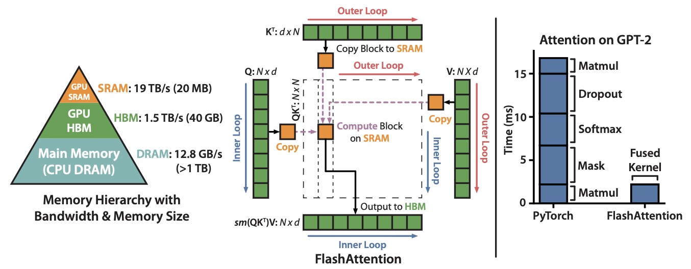
The figure below from the paper shows: (Left) FlashAttention uses tiling to prevent materialization of the large $N \times N$ attention matrix (dotted box) on (relatively) slow GPU HBM. In the outer loop (red arrows), FlashAttention loops through blocks of the $K$ and $V$ matrices and loads them to fast on-chip SRAM. In each block, FlashAttention loops over blocks of $Q$ matrix (blue arrows), loading them to SRAM, and writing the output of the attention computation back to HBM. Right: Speedup over the PyTorch implementation of attention on GPT-2. FlashAttention does not read and write the large $N \times N$ attention matrix to HBM, resulting in an 7.6x speedup on the attention computation.

Code
A detailed discourse on this topic is available in our FlashAttention primer.

FlashAttention-2

Proposed in FlashAttention-2: Faster Attention with Better Parallelism and Work Partitioning by Dao from Princeton and Stanford.
Scaling Transformers to longer sequence lengths has been a major problem in the last several years, promising to improve performance in language modeling and high-resolution image understanding, as well as to unlock new applications in code, audio, and video generation. The attention layer is the main bottleneck in scaling to longer sequences, as its runtime and memory increase quadratically in the sequence length.
FlashAttention exploits the asymmetric GPU memory hierarchy to bring significant memory saving (linear instead of quadratic) and runtime speedup (2-4x compared to optimized baselines), with no approximation. However, FlashAttention is still not nearly as fast as optimized matrix-multiply (GEMM) operations, reaching only 25-40% of the theoretical maximum FLOPs/s.
They observe that the inefficiency is due to suboptimal work partitioning between different thread blocks and warps on the GPU, causing either low-occupancy or unnecessary shared memory reads/writes.
This paper by Dao from Princeton and Stanford proposes FlashAttention-2, with better work partitioning to address these issues. In particular, they (1) tweak the algorithm to reduce the number of non-matmul FLOPs, (2) parallelize the attention computation, even for a single head, across different thread blocks to increase occupancy, and (3) within each thread block, distribute the work between warps to reduce communication through shared memory. These yield around 2x speedup compared to FlashAttention, reaching 50-73% of the theoretical maximum FLOPs/s on A100 and getting close to the efficiency of GEMM operations.
They empirically validate that when used end-to-end to train GPT-style models, FlashAttention-2 reaches training speed of up to 225 TFLOPs/s per A100 GPU (72% model FLOPs utilization).
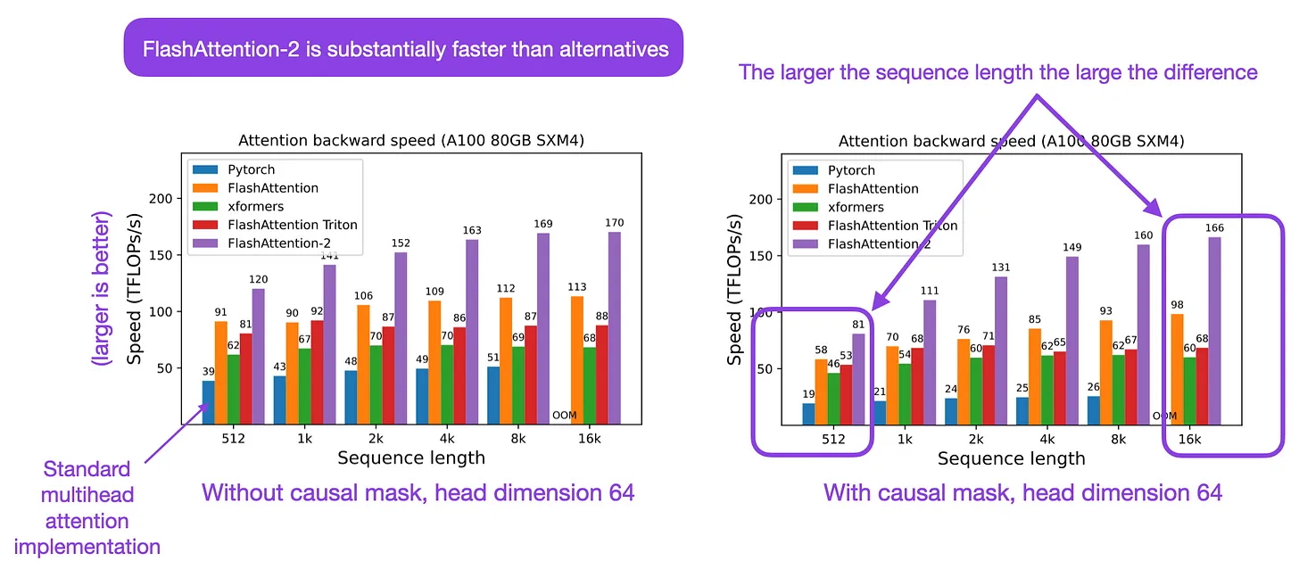
The following figure from Sebastian Raschka summarizes FlashAttention-2:

FlashAttention-3: Fast and Accurate Attention with Asynchrony and Low-precision

Proposed in FlashAttention-3: Fast and Accurate Attention with Asynchrony and Low-precision by Shah et al. from Colfax Research, Meta, NVIDIA, Georgia Tech, Princeton University, and Together AI.
FlashAttention-3 is an optimized attention mechanism for NVIDIA Hopper GPUs (H100), achieving significant speedups and accuracy improvements by exploiting hardware asynchrony and FP8 low-precision capabilities.
Key Contributions:
- Producer–Consumer Asynchrony: Implements warp-specialized software pipelining with a circular shared-memory buffer, separating producer warps (data movement via TMA) and consumer warps (Tensor Core GEMMs), hiding memory and instruction latencies.
- GEMM–Softmax Overlap: Breaks sequential dependencies to pipeline block-wise $QK^\top$ and $PV$ GEMMs with softmax, using “pingpong” scheduling across warpgroups and intra-warpgroup 2-stage pipelining to keep Tensor Cores and special function units active simultaneously.
- FP8 Low-precision Support: Adapts FlashAttention to FP8 WGMMA layout constraints via in-kernel transpose (using LDSM/STSM) and register permutations, and improves FP8 accuracy with block quantization and incoherent processing using random orthogonal transformations.
Architecture and Implementation:
- Input: Query ($Q$), Key ($K$), Value ($V$) matrices partitioned into tiles; head dimension $d$, sequence length$N$, query block size $B_r$, key block size$B_c$.
- Forward Pass (FP16):
  - Producer warps: Load $Q_i$, then sequentially load$K_j$, $V_j$ tiles from HBM to SMEM using TMA, notifying consumers via barriers.
  - Consumer warps: Perform SS-GEMM ($Q_iK_j^\top$), row-wise max tracking, local softmax, RS-GEMM ($\tilde{P}_{ij}V_j$), with scaling for stability, writing $O_i$ and log-sum-exp values $L_i$ to HBM.
  - Pipelined version: Overlaps GEMM from iteration $j$ with softmax from iteration $$j+1$, requiring extra register buffers ($S_{\text{next}}$).
- FP8 Mode:
  - Layout handling: Ensures k-major operand layout for $V$ in second GEMM by in-kernel transpose; register permutation aligns FP32 accumulators with FP8 operand layout.
  - Quantization: Block-level scaling (per $B_r\times d$ or $B_c\times d$ tile) and incoherent processing (Hadamard + random $\pm1$ diagonal matrices) reduce RMSE for outlier-heavy tensors.
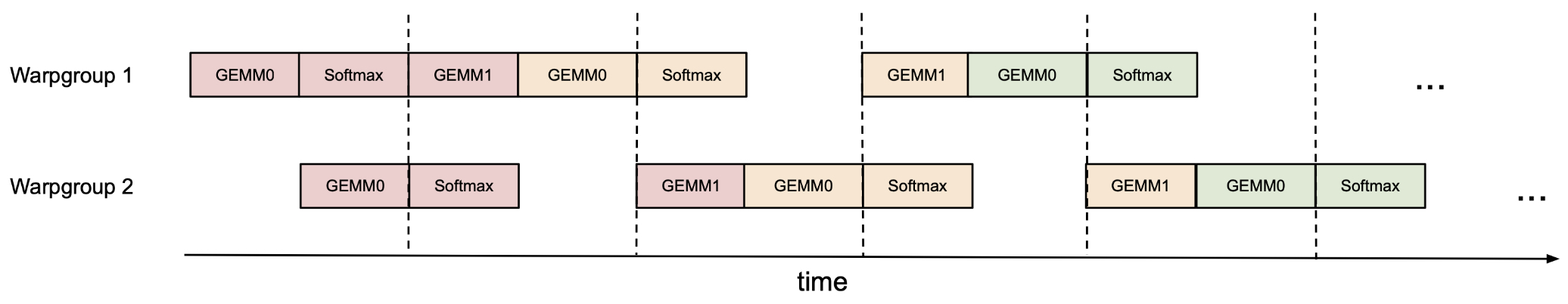
- The following figure from the paper shows ping‑pong scheduling for 2 warpgroups to overlap softmax and GEMMs: the softmax of one warpgroup should be scheduled when the GEMMs of another warpgroup are running. The same color denotes the same iteration.
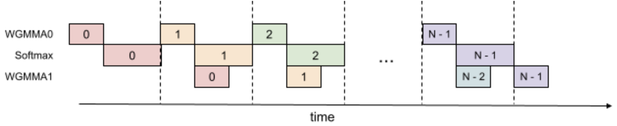
- The following figure from the paper shows 2-stage WGMMA-softmax pipelining.
Benchmarks:
- On H100 SXM5, FP16 forward pass reaches up to 740 TFLOPs/s (75% utilization), 1.5–2.0× faster than FlashAttention-2, and 3–16× faster than standard attention; backward pass sees 1.5–1.75× speedup.
- FP8 forward pass approaches 1.2 PFLOPs/s, outperforming cuDNN for some head dimensions and sequence lengths.
- Accuracy: FP16 matches FlashAttention-2 error ($\approx 1.9\times 10^{-4}$$ RMSE), both outperforming standard FP16 attention; FP8 with both block quantization and incoherent processing achieves 2.6× lower RMSE than baseline FP8 per-tensor scaling.
Ablation Studies:
- Removing GEMM–softmax pipelining or warp specialization reduces throughput from 661 TFLOPs/s to ~570–582 TFLOPs/s.
- Both optimizations contribute substantially to the performance gains.
Code

Multi-Query Attention (MQA)

Proposed in Fast Transformer Decoding: One Write-Head is All You Need.
Multi-head attention layers, as used in the Transformer neural sequence model, are a powerful alternative to RNNs for moving information across and between sequences. While training these layers is generally fast and simple, due to parallelizability across the length of the sequence, incremental inference (where such paralleization is impossible) is often slow, due to the memory-bandwidth cost of repeatedly loading the large “keys” and “values” tensors.
This paper by Shazeer from Google in 2019 proposes a variant called Multi-Query Attention (MQA), where the keys and values are shared across all of the different attention “heads”, greatly reducing the size of these tensors and hence the memory bandwidth requirements of incremental decoding.
They verify experimentally that the resulting models can indeed be much faster to decode, and incur only minor quality degradation from the baseline.
A detailed discourse on this topic is available in our Attention primer.

Grouped-Query Attention (GQA)

Proposed inGQA: Training Generalized Multi-Query Transformer Models from Multi-Head Checkpoints.
MQA, which only uses a single key-value head, drastically speeds up decoder inference. However, MQA can lead to quality degradation, and moreover it may not be desirable to train a separate model just for faster inference.
This paper by Ainslie et al. from Google Research (1) proposes a recipe for uptraining existing multi-head language model checkpoints into models with MQA using 5% of original pre-training compute, and (2) introduces grouped-query attention (GQA), a generalization of multi-query attention (MQA) which uses an intermediate (more than one, less than number of query heads) number of key-value heads.
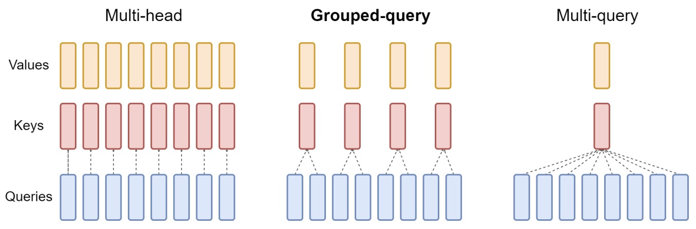
The following figure from the paper presents an overview of grouped-query method. Multi-head attention has $H$ query, key, and value heads. Multi-query attention shares single key and value heads across all query heads. Grouped-query attention instead shares single key and value heads for each group of query heads, interpolating between multi-head and multi-query attention.

MQA uses a single key-value head to speed up decoder inference but can lead to quality degradation. The authors propose a novel method to transform existing multi-head attention (MHA) language model checkpoints into models with MQA, requiring only 5% of the original pre-training compute.
The paper presents Grouped-Query Attention (GQA), an intermediate approach between multi-head and multi-query attention. In GQA, query heads are divided into groups, each sharing a single key and value head. This method allows uptrained GQA models to achieve near MHA quality with speeds comparable to MQA.
Experiments conducted on the T5.1.1 architecture across various datasets (including CNN/Daily Mail, arXiv, PubMed, MediaSum, Multi-News, WMT, and TriviaQA) show that GQA models offer a balance between inference speed and quality.
The study includes ablation experiments to evaluate different modeling choices, such as the number of GQA groups and checkpoint conversion methods. These provide insights into the model’s performance under various configurations.
The paper acknowledges limitations, such as evaluation challenges for longer sequences and the absence of comparisons with models trained from scratch. It also notes that the findings are particularly applicable to encoder-decoder models and suggests GQA might have a stronger advantage in decoder-only models.
They show that uptrained GQA achieves quality close to multi-head attention with comparable speed to MQA.
A detailed discourse on this topic is available in our Attention primer.

Linear Attention

Proposed in Linformer: Self-Attention with Linear Complexity by Wang et al. from Facebook AI.
The authors proposes a novel approach to optimizing the self-attention mechanism in Transformer models, reducing its complexity from quadratic to linear with respect to sequence length. This method, named Linformer, maintains competitive performance with standard Transformer models while significantly enhancing efficiency in both time and memory usage.
Linformer introduces a low-rank approximation of the self-attention mechanism. By empirically and theoretically demonstrating that the self-attention matrix is of low rank, the authors propose a decomposition of the original scaled dot-product attention into multiple smaller attentions via linear projections. This factorization effectively reduces both the space and time complexity of self-attention from $O(n^2)$ to $O(n)$, addressing the scalability issues of traditional Transformers.
The model architecture involves projecting key and value matrices into lower-dimensional spaces before computing the attention, which retains the model’s effectiveness while reducing computational demands. The approach includes options for parameter sharing across projections, which can further reduce the number of trainable parameters without significantly impacting performance.
In summary, here’s how Linformer achieves linear-time attention:
1. Low-Rank Approximation: The core idea behind Linformer is the observation that self-attention can be approximated by a low-rank matrix. This implies that the complex relationships captured by self-attention in Transformers do not necessarily require a full rank matrix, allowing for a more efficient representation.
2. Reduced Complexity: While standard self-attention mechanisms in Transformers have a time and space complexity of $O(n^2)$ with respect to the sequence length (n), Linformer reduces this complexity to $O(n)$. This significant reduction is both in terms of time and space, making it much more efficient for processing longer sequences.
3. Mechanism of Linear Self-Attention: The Linformer achieves this by decomposing the scaled dot-product attention into multiple smaller attentions through linear projections. Specifically, it introduces two linear projection matrices $E_i$ and $F_i$ which are used when computing the key and value matrices. By first projecting the original high-dimensional key and value matrices into a lower-dimensional space ($n \times k$), Linformer effectively reduces the complexity of the attention mechanism.
4. Combination of Operations: The combination of these operations forms a low-rank factorization of the original attention matrix. Essentially, Linformer simplifies the computational process by approximating the full attention mechanism with a series of smaller, more manageable operations that collectively capture the essential characteristics of the original full-rank attention.
The figure below from the paper shows: (left and bottom-right) architecture and example of the proposed multihead linear self-attention; (top right) inference time vs. sequence length the various Linformer models.

Experimental validation shows that Linformer achieves similar or better performance compared to the original Transformer on standard NLP tasks such as sentiment analysis and question answering, using datasets like GLUE and IMDB reviews. Notably, the model offers considerable improvements in training and inference speeds, especially beneficial for longer sequences.
Additionally, various strategies for enhancing the efficiency of Linformer are tested, including different levels of parameter sharing and the use of non-uniform projected dimensions tailored to the specific demands of different layers within the model.
The authors suggest that the reduced computational requirements of Linformer not only make high-performance models more accessible and cost-effective but also open the door to environmentally friendlier AI practices due to decreased energy consumption.
In summary, Linformer proposes a more efficient self-attention mechanism for Transformers by leveraging the low-rank nature of self-attention matrices. This approach significantly reduces the computational burden, especially for long sequences, by lowering the complexity of attention calculations from quadratic to linear in terms of both time and space. This makes Linformer an attractive choice for tasks involving large datasets or long sequence inputs, where traditional Transformers might be less feasible due to their higher computational demands.
A detailed discourse on this topic is available in our Attention primer.

Longformer

Proposed in Longformer: The Long-Document Transformer.
Transformer-based models are unable to process long sequences due to their self-attention operation, which scales quadratically with the sequence length.
This paper by Beltagy et al. from Allen AI in 2020 seeks to address this limitation, by introducing the Longformer with an attention mechanism that scales linearly with sequence length (commonly called Sliding Window Attention in the field), making it easy to process documents of thousands of tokens or longer.
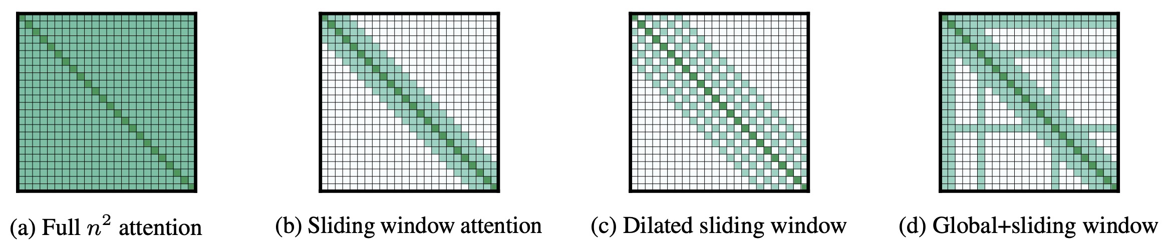
Longformer’s attention mechanism is a drop-in replacement for the standard self-attention and combines a local windowed attention with a task motivated global attention.
The figure below from the paper compares the full self-attention pattern and the configuration of attention patterns in Longformer.

Following prior work on long-sequence transformers, they evaluate Longformer on character-level language modeling and achieve state-of-the-art results on text8 and enwik8.
In contrast to most prior work, they also pretrain Longformer and finetune it on a variety of downstream tasks.
Their pretrained Longformer consistently outperforms RoBERTa on long document tasks and sets new state-of-the-art results on WikiHop and TriviaQA. They finally introduce the Longformer-Encoder-Decoder (LED), a Longformer variant for supporting long document generative sequence-to-sequence tasks, and demonstrate its effectiveness on the arXiv summarization dataset.
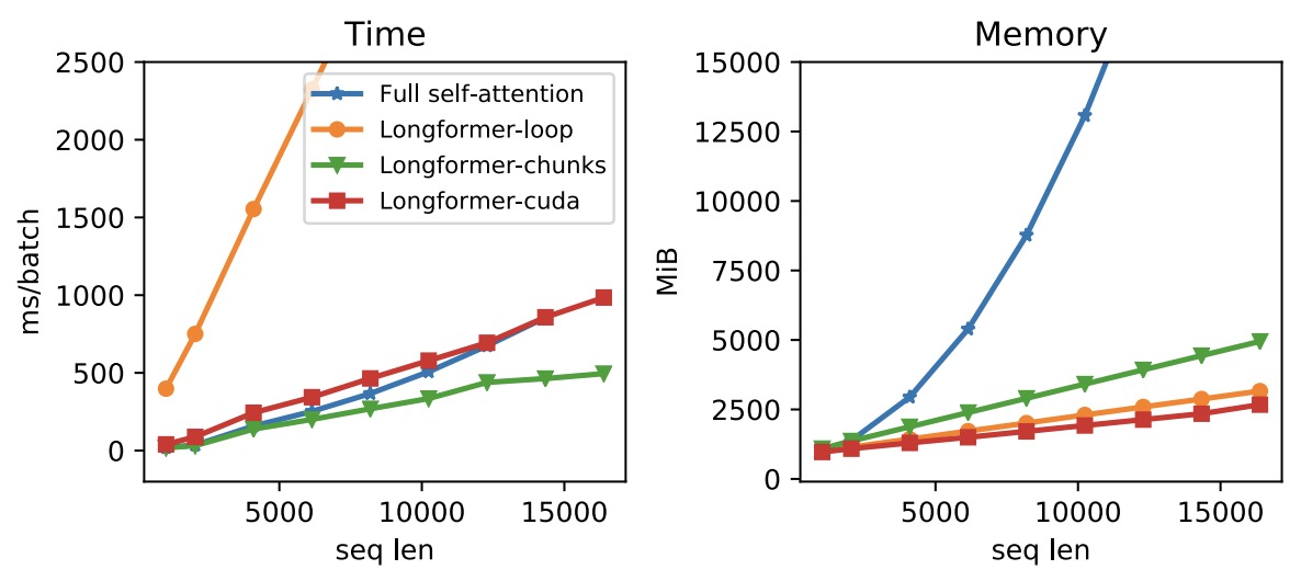
The figure below from the paper illustrates the runtime and memory of full self-attention and different implementations of Longformer’s self-attention; Longformer-loop is nonvectorized, Longformer-chunk is vectorized, and Longformer-cuda is a custom cuda kernel implementations. Longformer’s memory usage scales linearly with the sequence length, unlike the full self-attention mechanism that runs out of memory for long sequences on current GPUs. Different implementations vary in speed, with the vectorized Longformer-chunk being the fastest.

A detailed discourse on this topic is available in our Attention primer.

Inference Optimizations

Overview

Inference optimizations are a crucial area of research and engineering in the deployment of transformer models, particularly for real-time and resource-constrained environments. The goal is to minimize the computational cost and latency of running large language models (LLMs) without compromising their predictive accuracy. Optimizations during inference directly affect the responsiveness, scalability, and feasibility of these models in production systems.
One of the central challenges in inference is the autoregressive nature of many LLMs, where each token depends on the previously generated sequence. This leads to sequential dependencies that make naive inference expensive, especially for long sequences. To address this, a suite of optimization techniques has been developed to enhance the performance of transformer-based models during inference:
- KV Caching: The KV cache in transformer models is a critical optimization that enhances the efficiency and speed of sequence generation, making it a key component for deploying these models in real-world applications. The use of KV caching in autoregressive decoding processes, along with its role in latency optimization and scalability, makes it indispensable for serving transformer-based models efficiently. It allows previously computed key and value projections from self-attention layers to be stored and reused during subsequent decoding steps, avoiding redundant computations. This dramatically reduces per-token inference time beyond the first token, supports long-sequence generation, and is essential for achieving low-latency, high-throughput serving in applications like chat, streaming, and interactive agents.
- Model Quantization: Model quantization reduces the precision of weights and activations from 32-bit floating-point (float32) to lower-bit formats such as int8, float8, or even 4-bit representations like int4. This significantly cuts memory footprint and bandwidth usage, enabling deployment on smaller hardware and increasing throughput. Post-training quantization (PTQ) and quantization-aware training (QAT) are two common approaches. Quantized models benefit from faster matrix multiplications and lower energy consumption, and modern toolchains (e.g., NVIDIA TensorRT, Intel Neural Compressor) support hardware acceleration for quantized ops with minimal accuracy degradation.
- Operator Fusion: Operator fusion consolidates multiple sequential operations—such as linear projections, bias addition, layer normalization, and activation functions—into a single computational kernel. This reduces the number of memory read/write operations and kernel launch overhead on GPUs or TPUs, improving execution efficiency. For example, fusing a dense layer and a ReLU activation into a single fused kernel reduces latency and allows for more effective use of SIMD or CUDA cores, which are otherwise underutilized with fragmented ops.
- Speculative Decoding: Speculative decoding accelerates autoregressive generation by using a lightweight draft model to predict multiple future tokens in a single forward pass. These candidate tokens are then validated in parallel by the full, slower model. If validated, they are accepted en masse; otherwise, the generation rolls back. This pipeline reduces the number of expensive full-model invocations while maintaining generation fidelity. Approaches like Draft and Target Models, Medusa, Self-Speculative Decoding, FastRAG, and NVIDIA’s Speculative Decoding with Prefill leverage this technique to boost throughput while preserving model output quality.
- FlashAttention and Efficient Attention Kernels: FlashAttention is a memory-efficient attention algorithm that computes attention outputs in a tiled, fused, and GPU-friendly way, avoiding the need to materialize large intermediate attention matrices. It exploits GPU SRAM to keep frequently accessed blocks in high-speed memory and streams partial results to minimize memory bandwidth pressure. This approach scales better with sequence length and batch size than traditional softmax-based attention implementations. FlashAttention-2 and similar kernels (e.g., xFormers, Triton) are now standard in high-performance transformer inference stacks.
- Batching, Sequence Packing, and Prefilling:
- Batching groups multiple inference requests into a single execution pass, maximizing GPU utilization, amortizing kernel launch overhead, and improving throughput. Dynamic batching adapts to incoming request patterns, while token-level batching (e.g., vLLM) synchronizes decoding steps to serve many requests concurrently without blocking new ones.
- Sequence Packing minimizes padding waste by concatenating multiple short sequences into a single sequence tensor within a batch element, using an attention mask to prevent cross-sequence attention. This increases the density of useful tokens processed per batch, reducing memory footprint and improving effective throughput, especially in workloads with highly variable sequence lengths.
- Prefilling precomputes the KV cache for all prompt tokens before autoregressive decoding begins, avoiding redundant computation during generation. Optimizations like fused prefill kernels, prompt sharing, and layer-wise streaming further reduce latency in the prompt phase, which is often the most expensive stage for long inputs. Together, these three techniques ensure high hardware utilization, lower padding overhead, and minimized per-token computation cost.
- Prompt Caching: Caches the KV states of frequently used or repeated prompts—such as system instructions, few-shot exemplars, or user-defined templates—so they don’t need to be recomputed for each request. Particularly effective in chat or API-driven systems where the same initial context (e.g., “You are a helpful assistant…”) is used across sessions. By reusing prompt KV states, servers can skip prompt processing entirely and begin generation with the cache already initialized, significantly reducing time to first token and overall compute.
- Early Exit and Token Pruning: Early exit allows transformer layers to terminate inference for specific tokens when confidence thresholds or entropy-based stopping criteria are met, saving computation on later layers. Token pruning dynamically removes tokens or attention paths deemed irrelevant during inference, based on learned importance scores or gating functions. These techniques reduce compute costs without heavily sacrificing model output quality, and are especially useful for deployment scenarios where speed is prioritized over full precision.
- Hardware-Aware Scheduling: This optimization involves aligning inference workloads with the specifics of the underlying hardware—e.g., GPU memory hierarchy, tensor core availability, or pipeline concurrency. Scheduling strategies include operator placement, memory prefetching, stream prioritization, and load balancing across multi-GPU setups. For example, on NVIDIA GPUs, frameworks may utilize CUDA streams, shared memory, and kernel fusion to maximize throughput, while TPU inference may leverage XLA compilation for graph-level optimizations. Fine-tuned scheduling reduces contention, increases parallelism, and maximizes total inference throughput per watt.

KV Cache

Background: Self-Attention

In transformer models, each token attends to all previous tokens using a self-attention mechanism. For a sequence of input token embeddings $X \in \mathbb{R}^{T \cdot d}$, the transformer computes:
- Queries:
  \[Q = X W_Q\]
- Keys:
  \[K = X W_K\]
- Values:
  \[V = X W_V\]
- where $W_Q, W_K, W_V \in \mathbb{R}^{d \cdot d_k}$ are learned projection matrices, and $d_k$ is the head dimension.
The attention output is given by:
\[\text{Attention}(Q, K, V) = \text{softmax}\left( \frac{Q K^\top}{\sqrt{d_k}} \right) V\]
In a naive implementation, for each decoding step we must compute $K$ and $V$ for all tokens in the current sequence, across all layers. If $n$ is the number of tokens so far and $l$ is the number of layers, this requires $l \times (n−1)$ matrix multiplications per step, each of cost $O(d^2)$, leading to:
\[\text{Cost per token} = O(l \cdot n \cdot d^2)\]

Motivation

In the context of serving transformer models, the Key-Value (KV) cache is a core optimization technique for speeding up autoregressive decoding. It stores intermediate attention computations from previous decoding steps—specifically, the key and value tensors computed in the self-attention mechanism—so that they do not need to be recomputed at every new generation step. This dramatically reduces inference time and memory access overhead in LLMs, especially when generating long outputs.
Inference on transformers can be expensive because inference latency scales linearly with the number of layers $l$ in the model. A naive transformer implementation recomputes the $K$ and $V$ representations for all tokens in the sequence at each decoding step, across all layers, which is computationally heavy. Specifically, for a single attention head, the total cost per predicted token is:
\[O(l \cdot n \cdot d^2)\]
- where:
  - $n$ = number of tokens seen so far (sequence length)
  - $l$ = number of layers (depth)
  - $d$ = model (embedding) dimension
Without caching, predicting each new token involves:
1. Computing the key and value matrices for all past tokens and for every layer.
2. Performing matrix multiplications of the form:
\[K = X W_K, \quad V = X W_V\]
- where $X$ is the layer input and $W_K$, $W_V$ are fixed weight matrices.
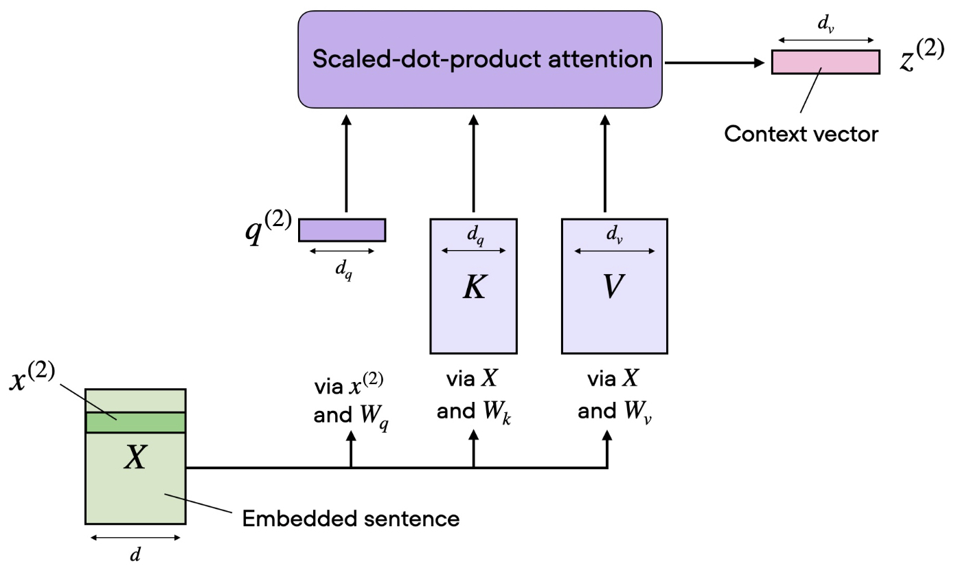
The KV cache optimization addresses this by reusing previously computed $K$ and $V$ representations, thus removing redundant computations for already processed tokens. This approach offers an $n$-times speedup in the sequence dimension, particularly impactful when $n$ is large.
The following figure (source) illustrates a typical self-attention block in transformers:

Self-Attention Block

Structure and Size of the KV Cache

The KV cache stores the key and value tensors for each transformer layer, attention head, the sample indices within each batch, and the token prefix length (i.e., the number of tokens already processed, including the prompt and any previously generated tokens, not just the immediate past token).
Assuming a transformer with:
- Sequence length so far: $n$
- Number of layers: $l$
- Number of attention heads per layer: $h$
- Head dimension: $d_k$
- Batch size: $b$
The KV cache for the above setup would consist of two main tensors per layer:
1. A key tensor of shape $(b, h, n, d_k)$, which stores the projected keys $K$ for all past tokens.
2. A value tensor of shape $(b, h, n, d_k)$ which stores the projected values $V$ for all past tokens.
Since each layer requires its own copy of both ($K$ and $V$) tensors, the total number of stored elements is:

\[\text{Total elements} = 2 \cdot l \cdot b \cdot h \cdot n \cdot d_k\]

If we assume each element is stored in 16-bit floating point precision (float16), then the total KV cache size in bytes is:
\[\text{Size (bytes)} = 2 \cdot l \cdot b \cdot h \cdot n \cdot d_k \cdot 2\]
- where the final factor of 2 accounts for the 2 bytes per float16 element.
Example:
- For a model with $l = 32$ layers, $h = 32$ heads, $d_k = 128$, $b = 1$, and $= 1000$:
\[\text{Size} = 2 \cdot 32 \cdot 1 \cdot 32 \cdot 1000 \cdot 128 \cdot 2 = 524{,}288{,}000 \ \text{bytes} \ (\approx 500 \ \text{MB})\]
This shows that the KV cache can become a significant memory consumer for long sequences, which is why optimizations such as quantization or chunked attention are often used in large language model inference.

Caching Self-Attention Values

KV caching exploits two key properties:
1. The model weights ($W_K$ and $W_V$) are fixed during inference.
2. The $K$ and $V$ representations for a given token depend only on that token and the fixed weights — they do not change in future steps.
Therefore, once we compute the $K$ and $V$ representations for a given (token, layer, head) tuple, we can store them and reuse them in all subsequent decoding steps.
At decoding step $t$:
- Without caching: recompute $K_{1:n}$ and $V_{1:n}$ from scratch for all $t$ tokens.
- With caching: reuse $K_{1:(n-1)}$ and $V_{1:(n-1)}$ compute only the new $k_t$ and $v_t$ and append them to the cache.
The following figure (source) illustrates the KV caching process, showing how only the new token’s $K$ and $V$ are computed while the rest are reused:

KV Caching Illustration

This optimization changes the cost from $O(l \cdot n \cdot d^2)$ to $O(l \cdot d^2)$ per decoding step — an $n$-times speedup in the sequence dimension.
This improvement is particularly significant for long sequences, where $n$ can be in the thousands to millions.

Why Not Cache Prior Queries?

Only the most recent query $q_t$ is used in the self-attention operation (which is recomputed at every step because it depends on the most recent token’s embedding), so caching prior queries ($q_{1:(n-1)}$) offers no benefit.

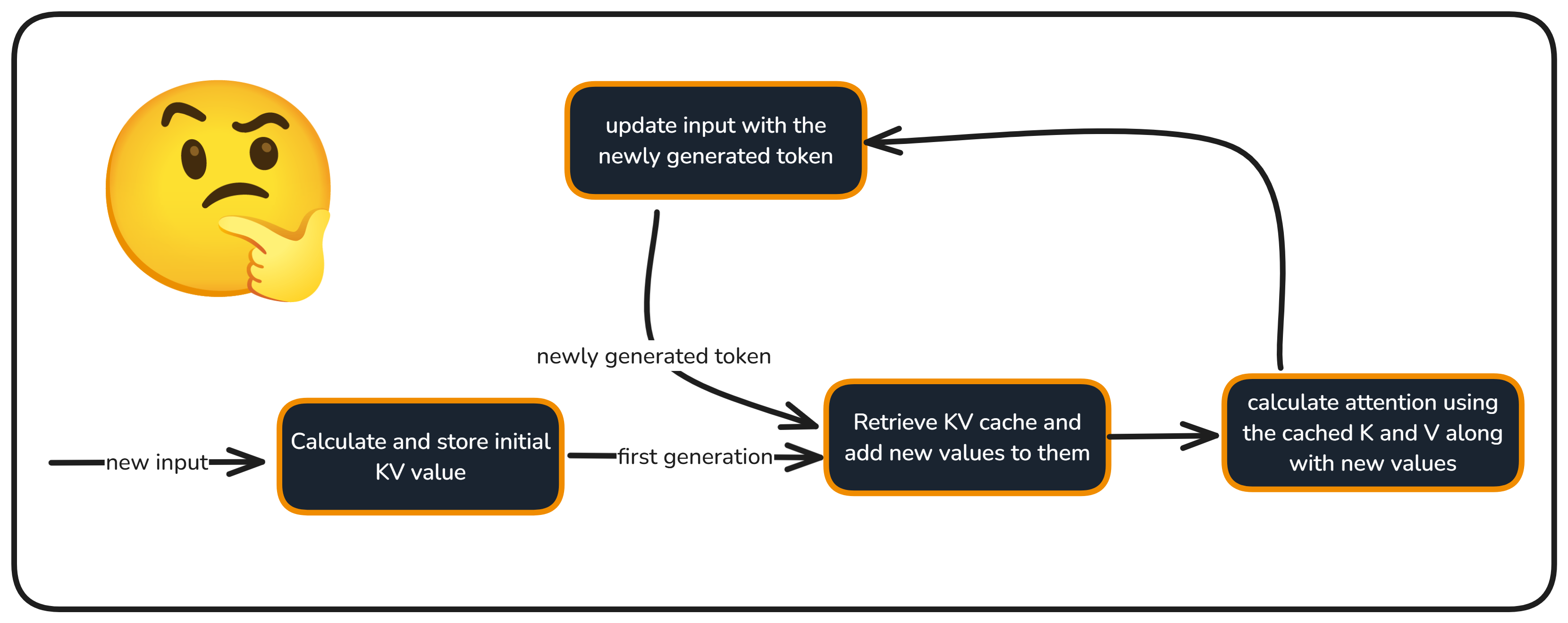
Autoregressive Decoding Process with Caching

Initial Sequence (Prefill Phase):
- Given a prompt sequence $S = [x_1, x_2, \dots, x_n]$ the model computes $K$ and $V$ tensors for all prompt tokens in all layers and stores them in the KV cache.
- This step still incurs the full cost $O(l \cdot n \cdot d^2)$ because we have no cached values yet.
- After this prefill step, the model transitions to the decode phase, where we process one token per step.
Predict Next Token:
- At decoding step $n+1$:
  - Compute the query vector $q_{n+1} = x_{n+1} W_Q$ for the new token.
  - Retrieve all previous keys and values from the cache:
  \[K_{1:n}, \; V_{1:n}\]
  - Compute the attention output for the new token using:
  \[\text{Attention}(q_{n+1}, K_{1:n}, V_{1:n})\]
Update Cache:
- Compute the new key and value vectors for the current token:
  \[k_{n+1} = x_{n+1} W_K, \quad v_{n+1} = x_{n+1} W_V\]
- Append these to the KV cache so they can be reused in future decoding steps:
  \[K_{\text{cache}} \leftarrow [K_{1:n}, k_{n+1}]\] \[V_{\text{cache}} \leftarrow [V_{1:n}, v_{n+1}]\]
Repeat:
- Continue until the end-of-sequence (EOS) token is generated or the maximum token limit is reached.

Implementation Details

Cache Tensor Shape

Assuming:
- Batch size $B$
- Max sequence length $n$
- Number of heads $H$
- Head dimension $d_k$
- Model (embedding) dimension $d$
- Number of layers $l$
The KV cache is structured to store $K$ and $V$ for each $(token, layer, head)$ tuple. In practice, the cache for a given layer and head has shapes:
- Key cache:
\[K_{cache} \in \mathbb{R}^{B \times H \times n \times d_k}\]
- Value cache:
  \[V_{cache} \in \mathbb{R}^{B \times H \times n \times d_k}\]
Since autoregressive generation processes one token per step in the decode phase, only 1 new key and value vector is appended at each step for each layer and head.
Efficient memory layout is crucial — contiguous buffers enable fast appends and reduce memory copy overhead.

Prefill Phase

When the prompt is first processed:
- The model computes $K$ and $V$ for all prompt tokens in every layer, filling the cache.
- This initial step has the same cost as the naive approach:
\[O(l \cdot n \cdot d^2)\]
After this, we move into the decode phase, where caching delivers the performance benefits.

Updates to the KV Cache

During autoregressive decoding, the $K$ and $V$ projections are cached for every processed token, across all layers and heads.
Each time a new token is generated:
1. The model computes $k_t$ and $v_t$ for that token in each layer.
2. These vectors are appended to the existing $K_{cache}$ and $V_{cache}$.
3. The updated cache is then used to compute the attention output for the next token.

Latency Optimization/Savings

Projection cost

Without caching:
- For a single head, at decoding step with sequence length $n$, the self-attention module recomputes $K$ and $V$ for all $n$ tokens across all $l$ layers.
- Computational cost per predicted token:
  \[O(l \cdot n \cdot d^2)\]
With caching:
- Only the key and value for the new token are computed, while the rest are reused from the cache.
- Computational cost per predicted token:
  \[O(l \cdot d^2)\]
This represents an $n$-times speedup in the sequence dimension. For large $n$ (e.g., thousands or millions of tokens), the cost reduction is dramatic.

Attention score computation

Without caching:
- At sequence length $n$, computing the attention scores requires multiplying the query for the new token with all $n$ keys. This is done for every layer, so the attention score computation cost per predicted token is:
  \[O(l \cdot n \cdot d)\]
- Because $n$ increases with each generated token, the latency for this step grows linearly in $n$ per token generation, but overall decoding (projection + attention) without caching still has quadratic growth in $n$.
With caching:
- Keys from all previous tokens are already stored. At sequence length $n$, we only compute the dot products between the new query and the cached keys:
  \[O(l \cdot n \cdot d)\]
- The cost per token still grows linearly with $n$, but caching removes the quadratic growth that comes from recomputing keys and values for older tokens.

Total complexity

KV caching transforms overall decoding latency from quadratic in $n$ to approximately linear in $n$, a major improvement for long-sequence generation. Specifically, KV caching changes the dominant scaling term from $O(n^2 \cdot d^2)$ to $O(n^2 \cdot d)$ which, for typical transformer sizes, is a substantial improvement in long-sequence latency. This is mathematically represented below.
Without caching:
- Total cost per predicted token = projection cost + attention score computation:
  \[O(l \cdot n \cdot d^2) + O(l \cdot n \cdot d) \approx O(l \cdot n \cdot d^2)\]
- Over an entire sequence of length n, the total decoding cost is:
  \[O(l \cdot n^2 \cdot d^2)\]
With caching:
- Total cost per predicted token = projection cost + attention score computation:
  \[O(l \cdot d^2) + O(l \cdot n \cdot d) \approx O(l \cdot n \cdot d)\]
- Over an entire sequence of length n, the total decoding cost is:
  \[O(l \cdot n^2 \cdot d)\]

Practical Deployment Considerations

Memory Management:
- Large caches for long sequences consume substantial GPU memory. Practical systems may:
  - Apply a sliding window to drop the oldest tokens.
  - Truncate caches for very long contexts to fit hardware limits.
Dynamic Batching:
- Batches often contain requests at different decoding stages. Each request must maintain its own KV cache state, and systems must efficiently manage per-request lookup and append operations.
Cache Parallelism:
- In multi-GPU serving:
  - KV caches may be partitioned across devices.
  - Synchronization strategies are needed to ensure all GPUs have the correct $K$ and $V$ for cross-device attention computations.

Multi-Head Attention and KV Cache

In practice, self-attention is implemented with multiple attention heads, each operating in a subspace of the embedding dimension. For head $h$ in $\{1, \dots, H\}$, we have:
\[Q^{(h)} = X W_{Q^{(h)}}, \quad K^{(h)} = X W_{K^{(h)}}, \quad V^{(h)} = X W_{V^{(h)}}\]
The attention outputs from each head are concatenated:
\[Q = \text{concat}(Q^{(1)}, Q^{(2)}, \dots, Q^{(H)})\]
- and similarly for $K$ and $V$.
Caching in multi-head attention:
- The KV cache stores keys and values for every head and every layer.
- Shape for the key and value cache:
\[K_{cache} \in \mathbb{R}^{B \times H \times T \times d_k}\] \[V_{cache} \in \mathbb{R}^{B \times H \times T \times d_k}\]
- where
  - $B$ = batch size (number of sequences processed in parallel)
  - $H$ = number of attention heads
  - $n$ = sequence length (number of tokens stored in the cache)
  - $d_k$ = dimension of the key (and value) vectors per head
Performance implications:
- Since each head’s KV cache is independent, the caching logic operates head-wise, but the storage is typically implemented as a unified tensor for efficiency.
- This unified tensor is arranged to be friendly to GPU tensor cores, enabling very fast read and write operations during decoding.
While KV caching greatly reduces the sequence dimension cost, the depth dimension (number of layers $l$) is still a significant contributor to compute. This leads to the KV Sharing idea, covered in detail in the section on KV Sharing — reusing $K$ and $V$ representations across the last half (or fraction) of layers to further cut computation. KV sharing builds on KV caching, but attacks the problem from the layer/depth dimension rather than the token dimension.

Summary of KV Cache Benefits

Reduces repeated computation by storing and reusing $K$, $V$ tensors instead of recomputing them at every step.
Enables efficient decoding in autoregressive generation by cutting per-step cost from $O(l \cdot n \cdot d^2)$ to $O(l \cdot d^2)$ — an $n$-times speedup in the sequence dimension.
Optimized for hardware acceleration via unified tensor layouts that are friendly to GPU tensor cores.
Scales well to large models and long contexts, with latency growing linearly rather than quadratically with sequence length.
Maintains accuracy because cached $K$ and $V$ are identical to recomputed values, given fixed weights.

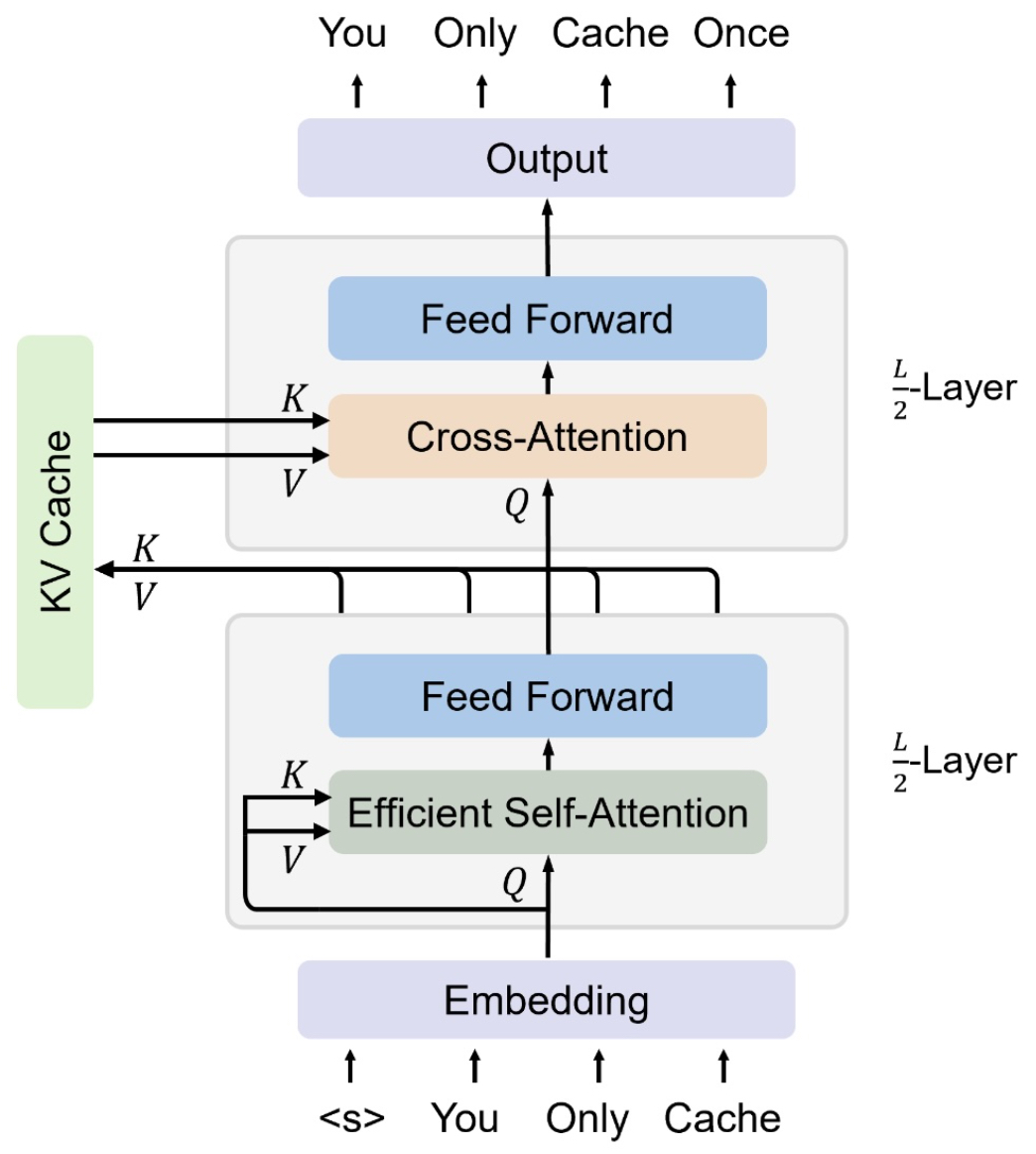
KV caching, introduced in You Only Cache Once: Decoder-Decoder Architectures for Language Models, optimizes the sequence dimension ($n$) cost, but the depth dimension ($l$) — the number of layers — still incurs full computation for each layer’s $K$ and $V$.
KV Sharing addresses this by reducing the cost of computing $K$ and $V$ along the depth dimension.
The intuition behind why this can work comes from studies such as Do Language Models Use Their Depth Efficiently? by Csordás et al., which show empirically that in a deep transformer-like model, the last layers are correlated with each other. This means the final few layers are not necessarily adding much new information, but rather tweaking the output produced so far. This redundancy can potentially be exploited to save computation without significantly degrading model quality.

The core idea: share actual $K$ and $V$ representations (not just weight matrices) across the last fraction of layers.
For example, if we share across the last half of the layers ($\frac{l}{2}$ layers):
1. The final layer before the shared region computes $K$ and $V$ normally.
2. All subsequent layers in the shared region reuse these $K$ and $V$ without recomputation, regardless of their inputs.
3. Other parameters (e.g., $W_Q$, MLP weights) remain distinct per layer.
Mathematically:
- Let $L_{share}$ be the index of the first shared layer.
- For any layer $j \geq L_{share}$:
\[K^{(j)} = K^{(L_{share})}, \quad V^{(j)} = V^{(L_{share})}\]
The following figure (source) illustrates KV Sharing across the last half of the layers, showing how a single computed $K$ and $V$ set is reused instead of recalculated:

KV Sharing Illustration

FLOP Savings

If the last $\frac{l}{k}$ layers share $K$ and $V$, we avoid computing them in $\frac{l}{k}$ layers entirely.
FLOP reduction: $\text{Savings} = \frac{\frac{l}{k}}{l} = \frac{1}{k}$ fraction of the total keys and values computation.
Combined with KV caching:
- KV caching cuts cost in $n$ (sequence) dimension.
- KV sharing cuts cost in $l$ (layer) dimension.

Empirical studies referenced in the paper show that in deep transformer models, the last few layers often produce correlated outputs.
This suggests that later layers are mostly fine-tuning rather than introducing fundamentally new information.
Reusing $K$ and $V$ in these layers therefore has minimal impact on output quality while significantly reducing compute and memory usage.

Memory Benefits

No need to store keys and values for the shared layers at all.
Reduces memory footprint in both inference and training.
Particularly valuable when serving long sequences, where cache size is dominated by $B \times H \times n \times d_k \times l$ scaling.

Deployment Notes

KV sharing must be considered at training time for best results, since models not trained with this constraint may suffer quality drops if sharing is applied post hoc.
Works alongside KV caching since KV sharing tackles depth, while KV caching tackles sequence length.

Model Quantization

Model quantization is a technique used to reduce the precision of numerical values (typically weights and activations) in a neural network from high-precision formats like 32-bit floating point (float32) to lower-precision formats such as int8, float8, or even int4. This allows for faster inference, reduced memory usage, and lower power consumption, particularly on hardware that supports low-precision arithmetic.
A detailed discourse on this topic is available in our Model Compression primer.

Why Quantize?

Quantization can lead to significant improvements in efficiency:
- Reduced Memory Footprint: An int8 model consumes 75% less memory than its float32 counterpart.
- Faster Arithmetic: Lower-precision operations (like int8 or int4 matmuls) are natively supported and highly optimized on modern accelerators (e.g., NVIDIA Tensor Cores, Intel AVX-512 VNNI).
- Lower Latency: With less data to move and faster compute kernels, quantized models offer reduced end-to-end inference time.

Types of Quantization

Post-Training Quantization (PTQ)

PTQ involves converting a pre-trained float32 model to a lower-precision model without retraining. It works by calibrating the ranges of tensors using a small sample of data.
Key steps in PTQ:
- Range Calibration: Identify the min/max values of weights and activations from a calibration dataset.
- Scale and Zero-Point Calculation: For each quantized tensor, calculate:
  \[q = \text{round}\left(\frac{r}{s}\right) + z\]
  - where:
    - $r$ is the real-valued number
    - $s$ is the scale (i.e., step size)
    - $z$ is the zero-point to preserve zero mapping in the quantized domain
    - $q$ is the quantized value (e.g., 8-bit integer)
Weight and Activation Clipping: Clip values to fit within the representable range of the target bit-width (e.g., [-128, 127] for signed int8).

Quantization-Aware Training (QAT)

QAT simulates quantization during training. Fake quantization layers are added to mimic low-precision computation while maintaining gradients in high precision.
Advantages:
- More accurate than PTQ for sensitive models (e.g., GPT, BERT).
- Allows the model to adapt to quantization errors during fine-tuning.
Implementation Details:
- Frameworks like PyTorch and TensorFlow include fake quantization modules (e.g., torch.quantization.FakeQuantize).
- Quant-dequant pairs are inserted in the model graph to simulate the behavior of actual quantized operations.

Static vs. Dynamic Quantization

Static Quantization: Activations are quantized ahead of time using calibration. Requires representative input data and is more performant but less flexible.
Dynamic Quantization: Weights are quantized ahead of time, but activations are quantized at runtime based on actual values. More flexible and easier to integrate but slightly slower.

Quantization in Transformers

In transformer models like GPT or BERT, quantization is applied to:
- Linear layers: Including query, key, value, and output projections in attention layers.
- GEMM-heavy blocks: MLP (feed-forward) layers.
- Embedding layers: Often quantized with special handling to preserve lookup efficiency.
Special Considerations:
- LayerNorm and Softmax are sensitive to quantization and often kept in float32.
- Attention scores may require FP16 or float32 to avoid instability.
- Mixed-precision quantization (e.g., float8 weights with int8 activations) is sometimes used.

Tooling and Frameworks

NVIDIA TensorRT / FasterTransformer
Intel Neural Compressor (INC)
PyTorch Quantization Toolkit
ONNX Runtime Quantization
BitsAndBytes (for 8-bit and 4-bit LLMs)
These tools offer end-to-end pipelines for quantizing, validating, and deploying models.

Operator Fusion

Operator fusion is an inference optimization technique that combines multiple adjacent operations in a neural network computation graph into a single composite operation. This is done to reduce overhead from memory reads/writes, kernel launches, and inter-operation communication, especially on GPU- or TPU-based systems.
Fusion reduces latency and increases compute efficiency by keeping data in faster registers or shared memory, rather than flushing it out to slower global memory between every small operation.

Motivation

Modern deep learning workloads often involve many small operations executed sequentially—e.g., matrix multiplications followed by bias addition, normalization, and non-linear activations:

\[x \rightarrow Linear \rightarrow Add Bias \rightarrow LayerNorm \rightarrow ReLU\]

Each of these operations might otherwise be implemented as a separate kernel. This leads to:
- Increased kernel launch overhead.
- Inefficient use of GPU parallelism.
- Repeated memory access and latency.
- Limited optimization opportunities for compilers.
By fusing them, the computation becomes more compact, minimizing overhead and maximizing performance.

Common Fusion Patterns

Some of the most commonly fused sequences in transformer inference include:
- GEMM + Bias Add + Activation
  - Example: $Y = \text{ReLU}(X @ W + b)$
  - Typically fused in MLP layers.
- Residual Add + LayerNorm + Dropout
  - Used in transformer blocks.
- Query/Key/Value Linear Projections
  - Three Linear ops fused into a single matmul followed by splitting heads.
- Softmax + Masking
  - In attention, softmax is often fused with masking logic to avoid branch divergence on GPUs.

Fusion in Transformers

In transformer architectures, operator fusion is especially valuable in:
- Multi-Head Attention Blocks:
  - Combine Q/K/V projections and reshape + transpose logic into a single kernel.
  - Fuse attention score computation, masking, and softmax into one efficient operation.
- Feed-Forward Networks (FFNs):
  - Fuse two linear layers with intermediate activation (e.g., GELU or ReLU).

Implementation Details

Fusion can be implemented in several ways:

Graph-Level Fusion (Ahead-of-Time)

High-level compilers like XLA (for TensorFlow) or TorchScript (for PyTorch) can analyze the computational graph and fuse operations during compilation.
Example in PyTorch:

@torch.jit.script
def fused_layer(x, w1, b1, w2, b2):
    return F.relu(F.linear(x, w1, b1)) @ w2.T + b2

TorchScript may fuse linear + relu into a single kernel.

Kernel-Level Fusion (Runtime)

Frameworks like NVIDIA’s TensorRT and FasterTransformer include hand-written CUDA kernels that combine multiple operations (e.g., QKV projection + transpose + scale + matmul) in one pass.
Example: A fused transformer kernel might compute:

qkv = fused_linear_bias_act(x);  // one call
q, k, v = split_heads(qkv);      // internal fused transpose and reshape

This reduces global memory traffic and utilizes registers/shared memory for intermediate results.

3. Custom Kernel Generation

Libraries like TVM or Triton enable defining custom fused kernels in a hardware-optimized DSL. These can be compiled just-in-time for maximum throughput.
Example in Triton:

@triton.jit
def fused_gemm_relu(...):
    # Define fused matmul + bias + relu logic using GPU thread blocks

Performance Impact

Operator fusion can lead to:

30–50% improvement in latency for attention blocks.
Higher hardware utilization, especially on GPUs with tensor cores or vectorized ALUs.
Reduced memory bandwidth pressure, which is often the bottleneck in LLM inference.

Tooling and Ecosystem

TensorRT: Extensive fusion for transformer blocks.
FasterTransformer: Fused QKV and FFN kernels.
ONNX Runtime with Graph Optimizer: Automatic fusion passes.
TorchScript + FBGEMM: Fusion of linear + activation ops.
TVM / Triton: Customizable and tunable fusion kernels.

Speculative Decoding

Speculative decoding is an inference-time optimization technique designed to reduce the latency of autoregressive sequence generation in large language models (LLMs). Instead of generating one token at a time using the full, expensive model, speculative decoding uses a smaller, faster “draft” model to guess multiple tokens in parallel, then validates these guesses with the full “target” model. If the guesses are correct, they are accepted as part of the output. Otherwise, they are partially or fully discarded and recomputed.
This method maintains the output quality of the original model while significantly improving throughput.

Motivation

Autoregressive decoding is inherently sequential. In a naive setup, the model generates one token, then feeds it back as input to generate the next. This sequential loop introduces latency and becomes a bottleneck during long-form generation.
Let:
- $f$ be the full model (large, accurate but slow)
- $g$ be the draft model (smaller, less accurate but fast)
Naively, generation requires $T$ forward passes of $f$ for a sequence of $T$ tokens. Speculative decoding aims to reduce the number of times $f$ is called.

Basic Algorithm

Initialize Context: Use a prompt or previous tokens $x$.
Draft Generation: Use the draft model $g$ to generate a sequence of $k$ speculative tokens:
\[y_1, y_2, ..., y_k = g(x)\]
Validation: Use the full model $f$ to compute the log-probabilities $p_f(y_t \| x, y_1, ..., y_{n-1})$.
Accept or Reject Tokens:
- Accept as many tokens as $f$ agrees with (within a confidence threshold or by matching top-1 outputs).
- Rewind to the last agreed-upon token and resume with the draft model from there.

Pseudocode

x = initial_prompt
while not done:
    draft_tokens = g.generate_next_k(x)
    probs_f = f.get_probs(x + draft_tokens)
    accepted_prefix = match(draft_tokens, probs_f)
    x = x + accepted_prefix

Key Parameters

Draft Model Quality: Must be fast enough to justify speculative overhead but good enough to match the full model reasonably often.
Block Size $k$: Number of speculative tokens generated per iteration. Larger blocks = fewer full model calls, but higher risk of rejection.
Matching Strategy: Usually uses top-1 match or a log-prob threshold.

Mathematical View

Let the probability of accepting each token be $\alpha$. Then the expected number of full-model calls is:

\[\mathbb{E}[\text{full passes}] \approx \frac{T}{k \cdot \alpha}\]

If $\alpha \approx 0.7$ and $k = 4$, we reduce full-model calls by nearly 3$\times$.

Implementation Details

Parallel Calls: $f$ can validate all $k$ tokens in one forward pass by using cached KV states and batched logits.
KV Cache Management: Efficient speculative decoding updates the cache only after validation.
Multimodel Serving: Systems like NVIDIA’s FasterTransformer or Hugging Face’s transformers can host both $f$ and $g$ concurrently with shared memory or GPU residency.

Notable Variants

Medusa (Meta): Uses a tree-structured decoder to validate multiple candidates at once.
FastRAG: Combines speculative decoding with retrieval-based models.
Draft & Verify (Google): A formalized framework for plug-and-play speculative decoding with checkpointing.

Benefits

Latency Reduction: 2$\times$–4$\times$ speedup in decoding for long sequences.
Full-Model Accuracy: Final output matches the output of the full model $f$, so there’s no accuracy loss.
Compatibility: Can be layered on top of existing decoding strategies (e.g., greedy, top-k, nucleus).

Limitations

Requires additional memory and compute for the draft model.
Effectiveness depends on alignment between the draft and full model distributions.
Complex cache management and integration overhead.

FlashAttention and Efficient Attention Kernels

In transformer models, self-attention is a core operation that enables the model to learn relationships between tokens. However, traditional attention implementations scale poorly with sequence length due to quadratic memory and compute complexity. FlashAttention and other efficient attention kernels address these bottlenecks by optimizing the attention computation to reduce memory overhead and improve performance.

Motivation

The standard attention computation involves the following operations for a sequence of length $L$ and hidden dimension $d$:
\[\text{Attention}(Q, K, V) = \text{softmax}\left(\frac{QK^T}{\sqrt{d}}\right) V\]
This requires:
- Computing a full $L \times L$ attention matrix (expensive for long sequences).
- Storing intermediate results like logits and softmax scores in global memory.
- Limited reuse of on-chip memory (registers, shared memory), resulting in bandwidth-bound performance.
FlashAttention addresses these inefficiencies by restructuring the attention algorithm to use memory-efficient block-wise computation.

FlashAttention: Key Concepts

Originally proposed in Dao et al., 2022 in FlashAttention: Fast and Memory‑Efficient Exact Attention with IO‑Awareness, FlashAttention is a fused, tiled implementation of scaled dot-product attention that:
- Eliminates materialization of the full attention matrix: Avoids creating and storing the entire $L \times L$ attention score matrix in GPU memory. Instead, computes small blocks of logits on-chip, applies masking and softmax immediately, and discards them, drastically reducing memory usage for long sequences.
- Uses tiling to partition queries, keys, and values into small blocks that fit in GPU shared memory: Splits $Q$, $K$, and $V$ into manageable tiles (e.g., $64 \times 64$) that can be loaded into fast on-chip shared memory or registers. This improves memory locality, reduces global memory reads/writes, and allows the GPU to reuse loaded data for multiple computations within the block.
- Fuses softmax, scaling, masking, and matmul into a single kernel: Combines these operations into one GPU kernel to avoid storing intermediate results in memory. By performing scaling, masking, softmax computation, and the weighted sum with $V$ in a single pass, FlashAttention reduces memory bandwidth usage and improves computational efficiency.

High-Level Algorithm

Load a block of queries $Q_{i}$ and keys $K_{j}$ into shared memory.
Compute attention logits $\frac{Q_i K_j^T}{\sqrt{d}}$ for the block.
Apply mask and softmax in-place, updating the running sum of exponents and maximums for numerical stability.
Accumulate partial outputs $A_{i,j} = \text{softmax}(Q_i K_j^T / \sqrt{d}) V_j$ without storing intermediate attention matrices.
Repeat across blocks until the full result is computed.

Numerical Stability

To avoid numerical overflow when computing softmax in a block-by-block fashion, FlashAttention keeps running statistics for each query row:
- $m_i = \max_{j} z_{ij}$ — the maximum logit value seen so far for that row, used to shift logits and prevent large exponentials.
- $s_i = \sum_{j} \exp\left(z_{ij} - m_i\right)$ — the running sum of the shifted exponentials, which forms the softmax denominator.
As new blocks are processed, these values are updated using associative operations that merge current and previous block statistics without loss of precision. This ensures the final softmax is mathematically equivalent to computing it on the full $L \times L$ matrix, but without ever storing that matrix.

Implementation Details

Written as a custom CUDA kernel.
Uses shared memory to hold Q/K/V tiles and compute locally.
Optimized to run in mixed precision (e.g., FP16 or BF16) for speed and memory efficiency.
Compatible with dropout, masking, and rotary embeddings.

FlashAttention-2 Improvements

Adds support for non-causal attention, variable-length sequences, and better warp-level parallelism.
Removes redundant memory loads through more aggressive caching and loop unrolling.
Enables backward pass efficiency, making it useful not only for inference but also for training.

Other Efficient Kernels

xFormers (Meta): Modular attention implementations that support Flash, sparse, and memory-efficient variants.
Triton-based Attention: Enables easy definition of fused attention kernels using Triton’s GPU DSL.
PagedAttention (vLLM): Optimizes KV cache access for batch inference, reducing memory fragmentation and improving latency.

Performance Gains

FlashAttention reduces attention memory complexity from:
- $\mathcal{O}(L^2)$ to $\mathcal{O}(L)$ for memory consumption.
- Achieves 1.7–2.7$\times$ speedup on A100 GPUs for long sequence lengths (> 1k tokens).
- Maintains exact attention output (within floating-point precision), unlike approximate methods.

Use in Inference

FlashAttention is especially beneficial for:
- Long-context models (e.g., 4k to 128k tokens).
- Multi-head attention, where per-head memory use adds up quickly.
- Deployment on GPUs with large shared memory (e.g., NVIDIA A100, H100).

Integration

Supported in:
- Hugging Face Transformers via use_flash_attention_2=True
- PyTorch through custom CUDA extensions or Triton kernels
- DeepSpeed, FasterTransformer, and xFormers

Batching, Sequence Packing, and Prefilling

Batching and prefilling are inference-time optimization techniques that improve efficiency and throughput by better utilizing hardware and avoiding redundant computations. These are especially critical when serving LLMs in real-time or at high concurrency.

Batching

Batching refers to the process of grouping multiple inference requests into a single forward pass through the model. This increases hardware utilization, amortizes overhead, and reduces latency per request (on average), particularly on GPUs that are optimized for matrix-heavy workloads.

Motivation

Without batching, each request results in an under-utilized forward pass:
- Small input tensor $\rightarrow$ Poor occupancy/utilization of GPU cores
- High overhead per kernel launch
- Wasted memory bandwidth
Batching solves this by aligning multiple requests into a tensor of shape:
\[\text{Batch Tensor: } (B, L, d)\]
- where:
  - $B$ is batch size
  - $L$ is sequence length
  - $d$ is hidden dimension

Types of Batching

Static Batching: Requests are grouped together at fixed time intervals. Simple but less flexible.
Dynamic Batching: Requests are buffered and grouped at runtime based on heuristics like request arrival time, sequence length, or prompt similarity.
Token-Level Batching: Pioneered by vLLM, this groups sequences by shared decoding step instead of sequence. Supports long-running generation jobs without blocking new ones.
Asynchronous Batching: Uses request queues and a scheduler to decide when to batch based on hardware load.

Padding and Masking

Since sequences may vary in length, shorter ones are padded and masked accordingly. Padding increases memory cost but enables unified matrix operations.
Example:
- Sequence A: [Hello, how, are, you] $\rightarrow$ length 4
- Sequence B: [Hi] $\rightarrow$ length 1
- Batched input: [[Hello, how, are, you], [Hi, PAD, PAD, PAD]]

Performance Benefits

Higher throughput: GPUs can process large matrices in parallel.
Lower kernel launch overhead.
Amortized use of KV cache and memory bandwidth.

Sequence Packing

Sequence packing is an optimization that reduces padding overhead when batching variable-length sequences. Instead of padding all sequences in a batch to the maximum length, multiple shorter sequences are concatenated into a single continuous sequence within the same batch element.
This approach stores and processes only actual tokens, using an attention mask to ensure tokens from different original sequences do not attend to each other.

Example

Without packing:
```
[Hello, how, are, you, PAD, PAD, PAD]
[Hi, there, PAD, PAD, PAD, PAD, PAD]
```
- Memory usage: proportional to 7 tokens per sequence (including pads).
With packing:
```
[Hello, how, are, you, Hi, there]
```
- Plus a mask to block attention between you and Hi.

Benefits

Reduced memory footprint — fewer padding tokens stored and processed.
Better hardware utilization — higher effective sequence density in each batch.
Lower latency for mixed-length workloads — especially beneficial when many short sequences are served alongside long ones.

Trade-offs

Slight overhead in constructing and applying more complex attention masks.
May require specialized batching logic and kernel support for optimal performance.

Prefilling

Prefilling refers to the one-time computation of model activations (primarily KV cache) for the prompt or context tokens before autoregressive decoding begins.

Motivation

Transformer inference separates the process into:
1. Prompt Phase (Prefill): Process entire prompt to initialize the KV cache.
2. Generation Phase (Decode): Generate one token at a time using cached keys and values.
The prompt phase is significantly more expensive because it processes multiple tokens without caching, while the decode phase uses KV caching for each new token.

Prefilling Logic

Given a prompt of $n$ tokens:
- The model performs a full forward pass to compute attention outputs for all $n$ positions.
- During this, it initializes the KV cache tensors:
  \[K_{1:n}, V_{1:n}\]
- These are used in all subsequent generation steps to avoid recomputation.

Optimizations

Fused Prefill Kernels: Libraries like FasterTransformer use specialized kernels to batch and prefill KV caches in a single efficient pass.
Prompt Sharing: If multiple requests use the same prompt (e.g., “You are a helpful assistant…”), cache the prefilled results and reuse them across requests.
Layer-Wise Streaming: Some implementations stream KV cache population layer-by-layer to overlap computation and memory operations.

Real-World Use

In production systems:
- Prompt prefill is often the dominant source of latency, especially with long prompts (e.g., 1k+ tokens).
- Prefilling is not cacheable unless the prompt is reused. That’s where prompt caching comes in.
- Systems may delay decoding until all requests in a batch complete their prefill phase.

Performance Benefits

Avoids redundant computation across decoding steps.
Enables efficient reuse of memory and attention context.
Critical for long-context inference and multi-user serving.

Prompt Caching

Prompt caching is an inference-time optimization that reuses the computed key-value (KV) attention states for frequently occurring or repeated prompt tokens. It eliminates the need to recompute the prefill phase of autoregressive decoding, which is typically the most computationally expensive part of the inference pipeline for long prompts.
This technique is especially effective in systems with repeated system messages, user templates, or static few-shot examples.

Motivation

During autoregressive generation, transformer models process the prompt (or context) once to initialize the attention cache. For a prompt of length $n$, this involves a full forward pass through all transformer layers to compute the KV tensors:

\[K_{1:n}^{(l)}, V_{1:n}^{(l)} \quad \text{for all layers } l\]

This prefill step is expensive and must be repeated for every new request — even if the prompt is the same.
Observation: Many applications use identical or highly similar prompts repeatedly. For example:
- Instructional prompts like: “You are a helpful assistant.”
- Few-shot templates in customer support bots.
- System prompts in chat APIs.
Prompt caching avoids repeated prefill for these common contexts.

Basic Mechanism

Cache Initialization:
- Compute and store KV tensors for a given prompt:
  \[\text{KV}_{\text{prompt}} = f(\text{prompt})\]
- Store in memory or disk with a unique key (e.g., hash of token IDs).
Cache Lookup:
- For each incoming request, compute a cache key from its prompt.
- If a match is found, retrieve KV tensors instead of recomputing them.
Continue Decoding:
- Begin token-by-token generation using the cached KV state:
  \[\text{Generate}(x_{n+1} \mid \text{KV}_{\text{prompt}})\]

Implementation Details

Cache Granularity

Full Prompt Cache: Caches the entire KV cache of a prompt. Simple and effective but can use a lot of memory.
Prefix Sharing: If prompts differ by suffix (e.g., Prompt A + User 1 and Prompt A + User 2), share the KV prefix and compute only the delta.
Subgraph Caching: In more advanced systems, only the first few layers or tokens may be cached.

Cache Storage

In-Memory KV Cache: For maximum performance, use GPU or CPU memory with LRU eviction.
On-Disk Cache: Slower but scalable for cold-start scenarios.
Keyed by Hash: Tokenized input is hashed using SHA or CRC to form a cache key. Some systems normalize prompts before hashing.

Integration with Serving Systems

Requires cache-aware batch scheduling.
Works best when integrated with dynamic batching and token-level schedulers (e.g., vLLM).
May include cache warming: preloading common prompts at system startup.

Performance Impact

Let:
- $T_p$ = time to prefill prompt
- $T_d$ = time per token for decode
For long prompts (e.g., 1000+ tokens), $T_p \gg T_d$, so caching the prefill can save 80–95% of per-request compute for repeated prompts.

Applications

Chat APIs: System messages or few-shot exemplars remain fixed across turns.
Agent Frameworks: Tools like LangChain often replay the same template structure.
Batch Inference: Multi-user prompts often share context headers (e.g., “Summarize the following…”).

Limitations

Prompt cache is only useful for identical or prefix-matching prompts.
Memory usage scales with prompt length and cache size.
May add overhead for hash computation or miss rate handling.
Not helpful for fully dynamic, unique user inputs.

Early Exit and Token Pruning

Early exit and token pruning are inference-time optimizations designed to reduce computation in large transformer models by selectively skipping or trimming parts of the computation graph that have diminishing contribution to the final output. These methods exploit redundancy in token representations and layer-wise stability in transformer models.
Both techniques aim to speed up inference without significantly affecting model output quality, making them valuable in latency-sensitive or resource-constrained applications.

Early Exit

Early exit allows the model to stop processing certain tokens or even entire sequences at intermediate layers if the model’s confidence in the prediction is already high.

Motivation

Transformer models use a fixed number of layers (e.g., 24 or 96), but not all tokens require the full depth to make a confident prediction. For example, easily classifiable tokens (like punctuation or common stopwords) may converge earlier than rare or ambiguous tokens.

Mechanism

At each transformer layer $l$, evaluate a confidence metric based on the current token representation:

Entropy-Based Confidence:
- Compute the softmax output $p^{(l)}$ from the current logits.
- Compute entropy:
  \[H(p^{(l)}) = - \sum_i p_i^{(l)} \log p_i^{(l)}\]
- If entropy $<$ threshold, consider the prediction confident enough to exit.
Cosine Similarity to Previous Layer:
- If representation at layer $l$ is similar to layer $l-1$, the token may have converged.
Learned Gates:
- Add a small classification head to each layer to learn exit decisions during training (as in BranchyNet or LayerDrop approaches).

Implementation

Models like BERT with Early Exit (DEEPL) implement classifier heads at multiple depths.
Hugging Face transformers has prototype support for early exit in sequence classification.
Requires threshold tuning to balance accuracy and latency.

Benefits

Reduces average inference depth (e.g., from 24 layers to 12–16 for many tokens).
Saves computation for simpler or high-confidence examples.
Ideal for classification or QA tasks where tokenwise prediction is not necessary.

Limitations

Adds overhead from confidence computation at intermediate layers.
Not widely adopted in generation tasks due to sequential dependencies between tokens.

Token Pruning

Token pruning reduces the number of tokens that are propagated through the deeper layers of a transformer by identifying and removing tokens with low contextual importance.

Motivation

In many attention-based computations, some tokens contribute very little to the output. For example, padding tokens or tokens with low attention weights to the rest of the sequence.
Pruning these tokens saves compute in later layers, especially in long-context models or batch scenarios.

Mechanism

Attention-Based Pruning:
- Compute the attention score variance or total attention mass a token receives:
  \[\alpha_i = \sum_{j} \text{Attention}(x_i, x_j)\]
- Prune tokens with low total attention received or given.
Top-$k$ Token Selection:
- Keep only the top-$k$ most important tokens per head or per sequence based on learned importance scores.
Dynamic Thresholding:
- Use learned or rule-based thresholds to drop tokens whose impact is below a tunable cutoff.
Progressive Pruning:
- Start with full tokens, and prune more aggressively as layers go deeper.

Implementation

Typically done at attention module boundaries.
Can be combined with sparse attention mechanisms.
Token indices need to be tracked to reconstruct output or map back to the original sequence.

Benefits

Reduces computation in deeper layers, especially for long sequences.
Improves throughput with minimal impact on quality in summarization, QA, and retrieval tasks.
Can be applied during training for alignment with inference.

Limitations

May degrade quality if pruning is too aggressive or incorrectly calibrated.
Requires complex index tracking and masking logic.
Harder to apply in autoregressive settings where all tokens are sequentially dependent.

Tools and Research

DeLighT, LayerDrop, and EarlyBERT for early exit variants.
SparseFormer, Synthesizer, and Longformer introduce related token reduction ideas.
Hugging Face and NVIDIA’s Megatron support token pruning hooks in research branches.

Hardware-Aware Scheduling

Hardware-aware scheduling refers to a set of optimization strategies that tailor the execution of neural network inference to the specific architecture and performance characteristics of the underlying hardware—such as GPUs, TPUs, or specialized accelerators. These optimizations aim to improve compute throughput, memory utilization, and latency by orchestrating how and when operations are executed.
This is especially important for transformer inference, where workloads are large, heterogeneous (e.g., KV cache lookups, matrix multiplies, normalization), and sensitive to memory bandwidth and parallelism.

Motivation

Transformer inference involves many stages of computation and memory access:
- Matrix multiplications (GEMMs) in attention and feed-forward blocks.
- Data movement between layers and devices.
- KV cache management and resizing.
- Softmax, activation, and normalization operations.
Without careful scheduling, bottlenecks can emerge due to:
- Underutilized compute units (e.g., Tensor Cores).
- Memory stalls and cache thrashing.
- Synchronization overhead between layers or streams.
Hardware-aware scheduling optimizes these execution flows to keep the pipeline full and latency low.

Core Techniques

Stream Parallelism

Modern GPUs support multiple concurrent execution streams (e.g., via CUDA). In transformer inference:
- Use separate CUDA streams for different model stages (e.g., one for KV cache update, one for GEMM).
- Overlap memory copies (e.g., cudaMemcpyAsync) with compute to hide latency.

Example:

 cudaMemcpyAsync(..., stream1);
 cublasGemmEx(..., stream2);  // runs concurrently with stream1

Tensor Core Utilization

Tensor cores are specialized units in NVIDIA GPUs for low-precision matrix ops (e.g., float16, bfloat16, int8). To maximize their usage:
- Ensure all matrix multiplications are aligned to multiple-of-8 dimensions.
- Use fused kernels to eliminate intermediate float32 conversions.
- Prefer mixed-precision pipelines (AMP / float16) for higher throughput.
Libraries like cuBLAS, FlashAttention, and TensorRT handle these optimizations automatically when configured correctly.

Operator Placement and Reordering

Efficient inference scheduling may involve reordering or co-locating operations based on:
- Memory locality: Fuse or group operations that share data.
- Execution time: Prioritize long-running ops earlier in the pipeline.
- Device affinity: Keep frequently accessed data on the same GPU or chip.
Example: Run attention blocks first in multi-layer transformer if they dominate compute time, allowing FFNs to be prefetched concurrently.

KV Cache Management

Efficient KV cache handling is essential in decoder models:
- Paged KV Cache: Used in systems like vLLM, stores KV in contiguous memory pages and allows random-access updates.
- Memory Pools: Preallocate KV buffers for each request and reuse them to avoid memory fragmentation.
- Lazy Allocation: Delay cache instantiation until first generation step to save memory for short prompts.

Pipeline and Model Parallelism

In large-model deployments:
- Pipeline Parallelism: Distribute transformer layers across devices. Stage execution overlaps compute and communication.
- Tensor Parallelism: Split individual tensor dimensions (e.g., weights) across devices for large GEMMs.
Combined, these allow serving models with billions of parameters across multiple GPUs efficiently.

Custom Kernel Scheduling

Frameworks like Triton and TVM allow defining and tuning custom kernels:
- Auto-tune tiling sizes and shared memory usage.
- Schedule GPU threads based on warp/block-level parallelism.
- Implement custom token-wise or layer-wise scheduling logic.

Cache and Memory Prefetching

Use __prefetch instructions or async loads to bring data into shared memory before it is needed.
Overlap KV fetches with matmul execution to hide memory latency.

Deployment-Aware Strategies

Load Balancing: Use dynamic batching queues with GPU-aware request routing (e.g., based on latency or memory pressure).
Thread Affinity: Bind computation to specific CPU cores or NUMA zones in CPU-bound systems.
Execution Profiling: Use profilers like NVIDIA Nsight Systems or PyTorch Profiler to tune for bottlenecks.

Ecosystem Support

NVIDIA TensorRT and FasterTransformer: Hardware-aware fused kernels and scheduling policies.
ONNX Runtime (ORT): Execution providers tuned for different hardware (CUDA, DirectML, TensorRT).
DeepSpeed, vLLM, Triton, and TVM: Offer fine-grained control over scheduling and memory layout.

Performance Impact

Hardware-aware scheduling can yield:
- 1.5$\times$–4$\times$ speedup over naive scheduling for long sequences or large batches.
- Better multi-GPU scaling for high-throughput inference.
- Lower latency variability in real-time serving environments.

Comparative Analysis

Technique	Purpose	Key Benefits	Primary Use Cases	Implementation Notes
KV Caching	Reuse attention keys/values from previous tokens	Reduces per-token latency after first step	Autoregressive decoding (GPT, LLaMA)	Requires careful cache management; starts from second token onward
Model Quantization	Use lower-precision weights/activations	Reduces memory and compute cost	Edge inference, high-throughput serving	`int8`/PTQ for speed; QAT for better accuracy; needs hardware with quantization support
Operator Fusion	Combine adjacent ops into single kernel	Reduces memory access and kernel launch overhead	Attention blocks, FFNs, LayerNorm + activation	Use graph compilers (XLA, TorchScript), or fused CUDA kernels (TensorRT, FasterTransformer)
Speculative Decoding	Use draft model to guess multiple tokens	Reduces number of full-model forward passes	Long-form generation, chatbots	Needs a lightweight auxiliary model; uses top-1 match or log-prob threshold for validation
FlashAttention & Kernels	Memory-efficient attention computation	Reduces memory usage and boosts speed	Long-sequence LLMs, multi-head attention	Implemented with CUDA (FlashAttention), or Triton/xFormers; avoids storing full attention matrix
Batching	Process multiple requests together	Increases throughput and GPU utilization	High-concurrency inference (API servers, batch jobs)	Dynamic and token-level batching supported in vLLM, DeepSpeed, TensorRT
Prefilling	Precompute KV cache from prompt tokens	Avoids recomputation in autoregressive models	Chat and generation tasks with long prompts	Often paired with batching; prompt KV cache initialized before decoding begins
Prompt Caching	Cache KV states of repeated prompts	Saves time and compute on repeated static contexts	Chat APIs, few-shot prompt templates	Requires hashing/tokenizing prompt and storing cache; memory usage grows with cache diversity
Early Exit	Stop processing tokens/layers early based on confidence	Reduces per-token compute in deep models	Classification, QA tasks	Needs entropy or learned gating logic; difficult to apply in token-dependent generation
Token Pruning	Discard low-importance tokens during inference	Reduces sequence length in deeper layers	Long-sequence summarization, QA	Attention-based importance scoring; careful masking and index tracking required
Hardware-Aware Scheduling	Optimize kernel execution for specific hardware	Maximizes throughput and minimizes latency	All transformer-based workloads	Includes stream parallelism, memory prefetch, cache layout, tensor core tuning, and multi-GPU distribution

References

Citation

If you found our work useful, please cite it as:

@article{Chadha2020DistilledModelAcceleration,
  title   = {Model Acceleration},
  author  = {Chadha, Aman},
  journal = {Distilled AI},
  year    = {2020},
  note    = {\url{https://aman.ai}}
}

Training Optimizations

Overview

FlashAttention

FlashAttention-2

FlashAttention-3: Fast and Accurate Attention with Asynchrony and Low-precision

Multi-Query Attention (MQA)

Grouped-Query Attention (GQA)

Linear Attention

Longformer

Inference Optimizations

Overview

KV Cache

Background: Self-Attention

Motivation

Structure and Size of the KV Cache

Caching Self-Attention Values

Why Not Cache Prior Queries?

Autoregressive Decoding Process with Caching

Implementation Details

Cache Tensor Shape

Prefill Phase

Updates to the KV Cache

Latency Optimization/Savings

Projection cost

Attention score computation

Total complexity

Practical Deployment Considerations

Multi-Head Attention and KV Cache

Summary of KV Cache Benefits

KV Sharing

How KV Sharing Works

FLOP Savings

Why KV Sharing Can Work

Memory Benefits

Deployment Notes

Model Quantization

Why Quantize?

Types of Quantization

Post-Training Quantization (PTQ)

Quantization-Aware Training (QAT)

Static vs. Dynamic Quantization

Quantization in Transformers

Tooling and Frameworks

Operator Fusion

Motivation

Common Fusion Patterns

Fusion in Transformers

Implementation Details

Graph-Level Fusion (Ahead-of-Time)

Kernel-Level Fusion (Runtime)

3. Custom Kernel Generation

Performance Impact

Tooling and Ecosystem

Speculative Decoding

Motivation

Basic Algorithm

Pseudocode

Key Parameters

Mathematical View

Implementation Details

Notable Variants

Benefits

Limitations

FlashAttention and Efficient Attention Kernels

Motivation

FlashAttention: Key Concepts

High-Level Algorithm

Numerical Stability

Implementation Details

FlashAttention-2 Improvements

Other Efficient Kernels

Performance Gains

Use in Inference

Integration

Batching, Sequence Packing, and Prefilling

Batching

Motivation

Types of Batching

Padding and Masking

Performance Benefits