ML Algorithms Comparative Analysis
- Overview
- Classification Algorithms
- Regression Algorithms
- Classification and Regression Algorithms
- Clustering in Machine Learning: Latent Dirichlet Allocation and K-Means
- Summary
- Comparative Analysis: Linear Regression, Logistic Regression, Support Vector Machines, k-Nearest Neighbors, and k-Means
- References
- Citation
Overview
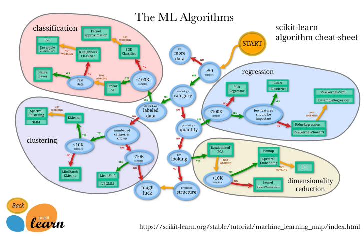
- The figure below (source) offers a deep dive on the pros and cons of the most commonly used regression and classification algorithms and the use-cases for each.
Classification Algorithms
Logistic Regression
- To start off here, Logistic Regression is a misnomer as it does not pertain to a regression problem at all.
- Logistic regression estimates the probability of an event occurring based on a given dataset of independent variables. Since the outcome is a probability, the dependent variable is bounded between 0 and 1.
- You can use your returned value in one of two ways:
- You may just need an output of 0 or 1 and use it “as is”.
-
Say your model predicts the probability that your baby will cry at night as:
\[p(cry|night)= 0.05\] -
Let’s leverage this information to see how many times a year you’ll have to wake up to soothe your baby:
\[\begin{align} wakeUp &= p(cry|nights)*nights \\ &= 0.05 * 365 \\ &= 18 \text{ days} \end{align}\]
-
- Or you may want to convert it into a binary category such as: spam or not spam and convert it to a binary classification problem.
- In this scenario, you’d want an accurate prediction of 0 or 1 and no probabilities in between.
- The best way to obtain this is by leveraging the sigmoid function as it guarantees a value between 0 and 1.
- Sigmoid function is represented as:
\[y^{\prime}=\frac{1}{1+e^{-z}}\]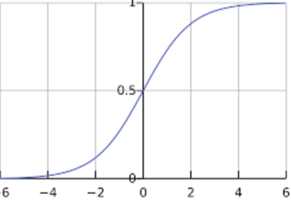
- where,
- \(y^{\prime}\) is the output of the logistic regression model for a particular example.
- The \(w\) values are the model’s learned weights, and \(b\) is the bias.
- The \(x\) values are the feature values for a particular example.
- You may just need an output of 0 or 1 and use it “as is”.
- Pros:
- Algorithm is quite simple and efficient.
- Provides concrete probability scores as output.
- Cons:
- Bad at handling a large number of categorical features.
- It assumes that the data is free of missing values and predictors are independent of each other.
- Use case:
- Logistic regression is used when the dependent variable (target) is categorical as in binary classification problems.
- For example, To predict whether an email is spam (1) or (0) or whether the tumor is malignant (1) or not (0).
- Logistic regression is used when the dependent variable (target) is categorical as in binary classification problems.
Naive Bayes Classifier
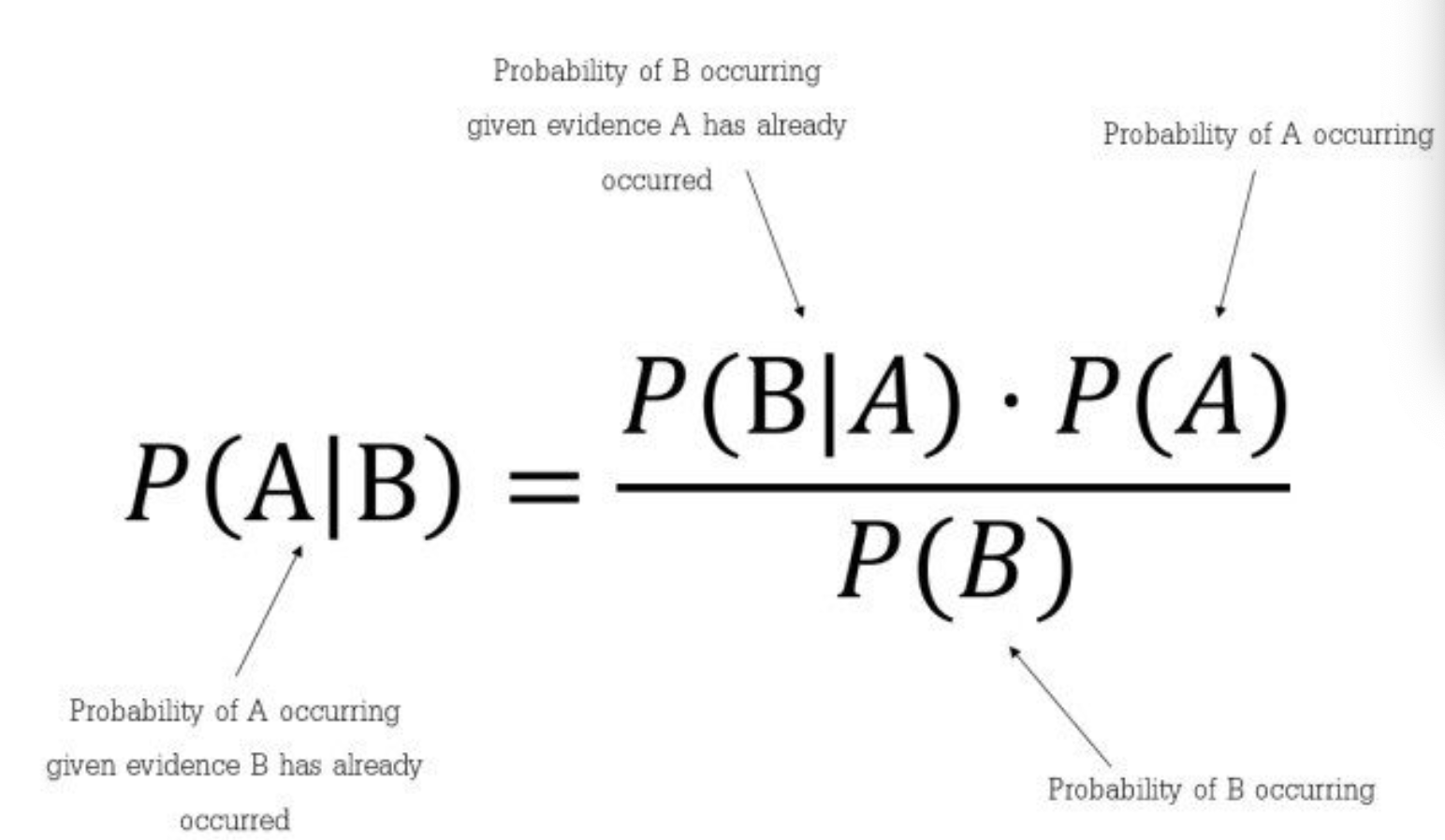
- Naive Bayes is a supervised learning algorithms based on Bayes’ theorem which can serve as either a binary or multi-class classifier.
- It is termed “naive” because it makes the naive assumption of conditional independence between every pair of features given the value of the class variable.
- The figure below below (source) shows the equation for Bayes Theorem and its individual components:
-
The thought behind naive Bayes classification is to try to classify the data by maximizing:
\[P(O \mid C_i) P(C_i)\]- where,
- \(O\) is the object or tuple in a dataset.
- \(i\) is an index of the class.
- where,
- Pros:
- Under-the-hood, Naive Bayes involves a multiplication (once the probability is known) which makes the algorithm simplistic and fast.
- It can also be used to solve multi-class prediction problems.
- This classifier performs better than other models with less training data if the assumption of independence of features holds.
- Cons:
- It assumes that all the features are independent. This is actually a big con because features in reality are frequently not fully independent.
- Use case:
- When the assumption of independence holds between features, Naive Bayes classifier typically performs better than logistic regression and requires less training data.
- It performs well in case of categorical input variables compared to continuous/numerical variable(s).
Regression Algorithms
Linear Regression
- Linear regression analysis is a supervised machine learning algorithm that is used to predict the value of an output variable based on the value of an input variable.
- The output variable we’re looking to predict is called the dependent variable.
- The input variable we’re using to predict the output variable’s value is called the independent variable.
- Assumes a linear relationship between the output and input variable(s) and fits a linear equation on the data.
- The goal of Linear Regression is to predict output values for inputs that are not present in the data set, with the belief that those outputs would fall on the fitted line.
- Pros:
- Performs very well for linearly separated data.
- Easy to implement and is interpretable.
- Cons:
- Prone to noise and overfitting.
- Very sensitive to outliers.
- Use case:
- Linear regression is commonly used for predictive analysis and modeling.
Classification and Regression Algorithms
k-Nearest Neighbors
- Based on the age-old adage “birds of a feather flock together”.
- The \(k\)-nearest neighbors algorithm, also known as \(k\)-NN, is a non-parametric, supervised machine learning algorithm, which uses proximity to make classifications or predictions about the grouping of an individual data point.
- While it can be used for either regression or classification problems, it is typically used as a classification algorithm, working off the assumption that similar points can be found near one another.
- The value of \(k\) is a hyperparameter which represents the number of neighbors you’d like the algorithm to refer as it generates its output.
- \(k\)-NN answers the question that given the current data, what are the \(k\) most similar data points to the query.
- \(k\)-NN calculates distance typically using either Euclidean or Manhattan distance:
-
Euclidean distance:
\[d(x, y)=\sqrt{\sum_{i=1}^{n}\left(y_{i}-x_{i}\right)^{2}}\] -
Manhattan distance:
\[d(x, y)=\sum_{i=1}^{m}\left|x_{i}-y_{i}\right|\]
- This is the high-level view of how the algorithm works:
- For each example in the data:
- Calculate distance between query example and current example from the data.
- Add the distance and index to an ordered collection.
- Sort in ascending order by distance.
- Pick first \(k\) from sorted order.
- Get labels of selected \(k\) entries.
- If regression, return the mean of \(k\) labels.
- If classification, return the majority vote (some implementations incorporate weights for each vote) of the labels.
- For each example in the data:
- Pros:
- Easy to implement.
- Needs only a few hyperparameters which are:
- The value of \(k\).
- Distance metric used.
- Cons:
- Does not scale well as it takes too much memory and data storage compared with other classifiers.
- Prone to overfitting if the value of \(k\) is too low and will underfit if the value of \(k\) is too high.
- Use case:
- While \(k\)-NNs can be used for regression problems, they are typically used for classification.
- When labelled data is too expensive or impossible to obtain.
- When the dataset is relatively smaller and is noise free.
Support Vector Machines
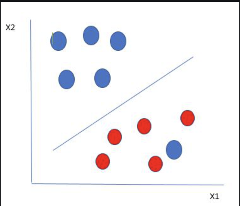
- The objective of Support Vector Machines (SVMs) is to find a hyperplane in an \(N\)-dimensional space (where \(N\) is the number of features) that distinctly classifies the data points.
- Note that a hyperplane is a decision boundary that helps classify the data points. If the number of input features is 2, hyperplane is just a line, if input features is 3, it becomes a 2D plane.
- The subset of training data points utilized in the decision function are called “support vectors”, hence the name Support Vector Machines.
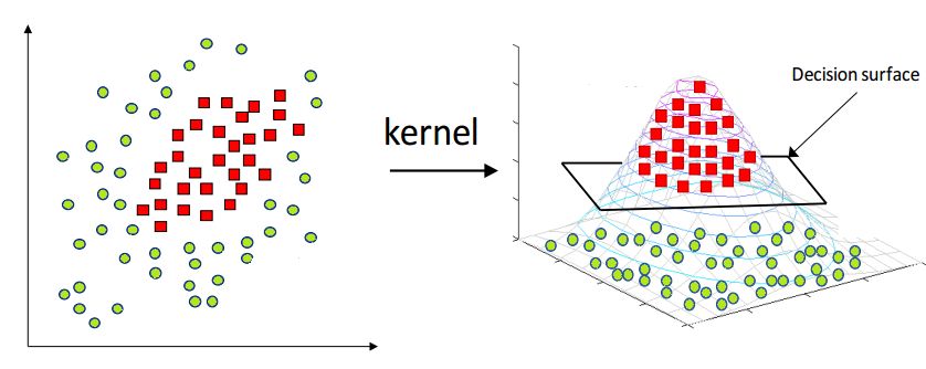
- In the instance that the data is not linearly separable, we need to use the kernel trick (also called the polynomial trick). The SVM kernel is a function that takes low dimensional input space and transforms it into higher-dimensional space, i.e., it enables learning a non-linear decision boundary to separate datapoints. The gist of the kernel trick is that learning a linear model in the higher-dimensional space is equivalent to learning a non-linear model in the original lower-dimensional input space. More on this in the article on SVM Kernel/Polynomial Trick.
- The image below (source) displays the linear hyperplane separating the two classes such that the distance from the hyperplane to the nearest data point on each side is maximized. This hyperplane is known as the maximum-margin hyperplane/hard margin.
- Pros:
- Effective in high dimensional spaces.
- Effective in cases where the number of dimensions is greater than the number of samples.
- Works well when there is a clear margin of separation between classes.
- Memory efficient as it uses a subset of training points in the decision function (“support vectors”).
- Versatile since different Kernel functions can be specified for the decision function. Common kernels are provided, but it is also possible to specify custom kernels.
- Cons:
- Doesn’t perform well when we have large datasets because the required training time is higher.
- If the number of features is much greater than the number of samples, avoiding over-fitting in choosing kernel functions and regularization term is crucial.
- SVMs do not directly provide probability estimates, these are calculated using an expensive five-fold cross-validation.
- Doesn’t perform very well when the dataset has more noise, i.e., when target classes are overlapping.
- Use case:
- While SVMs can be used for regression problems, they are typically used for classification (similar to \(k\)-NN) and outliers detection.
- Works great if the number of features is high and they occur in high dimensional spaces.
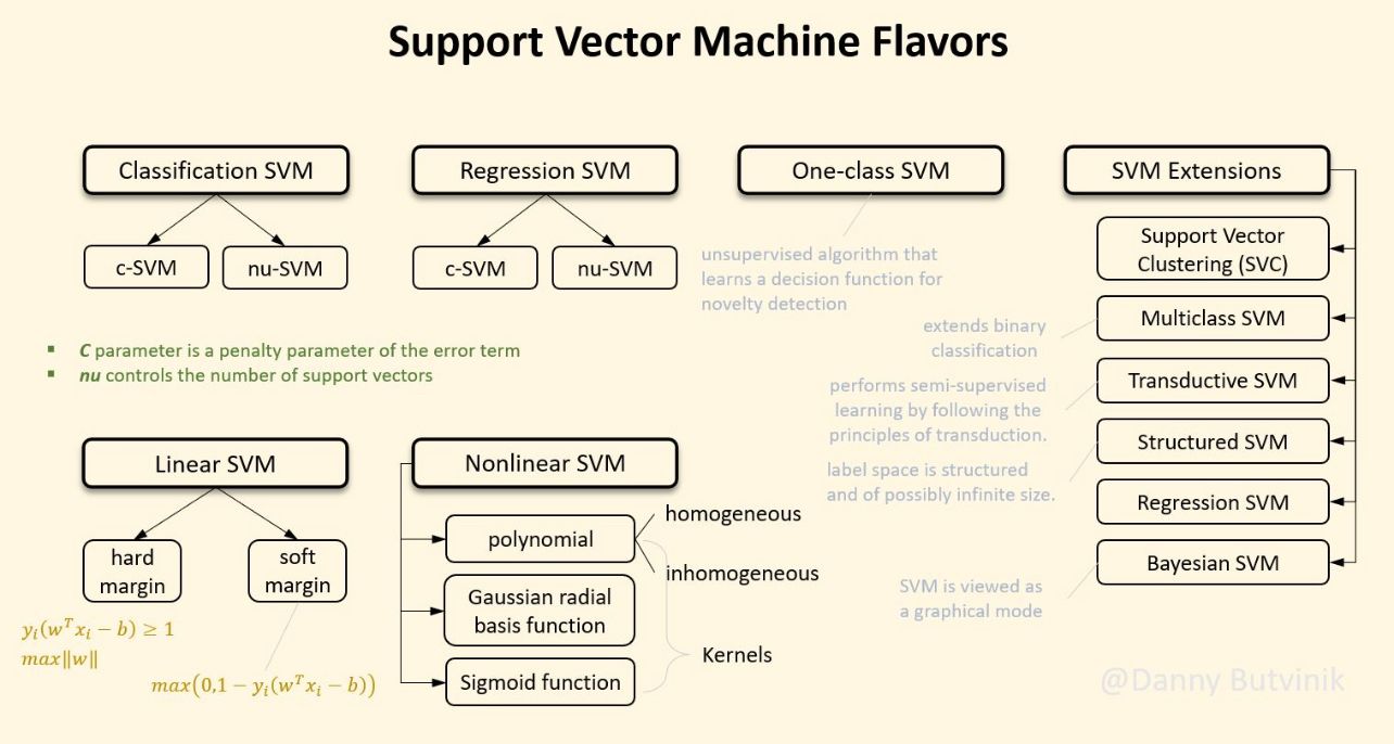
- The following figure (source) shows SVM flavors.
Explain the kernel trick in SVM and why we use it and how to choose what kernel to use?
- Kernels are used in SVM to map the original input data into a particular higher dimensional space where it will be easier to find patterns in the data and train the model with better performance.
- For e.g.: If we have binary class data which form a ring-like pattern (inner and outer rings representing two different class instances) when plotted in 2D space, a linear SVM kernel will not be able to differentiate the two classes well when compared to a RBF (radial basis function) kernel, mapping the data into a particular higher dimensional space where the two classes are clearly separable.
- Typically without the kernel trick, in order to calculate support vectors and support vector classifiers, we need first to transform data points one by one to the higher dimensional space, and do the calculations based on SVM equations in the higher dimensional space, then return the results. The ‘trick’ in the kernel trick is that we design the kernels based on some conditions as mathematical functions that are equivalent to a dot product in the higher dimensional space without even having to transform data points to the higher dimensional space. i.e we can calculate support vectors and support vector classifiers in the same space where the data is provided which saves a lot of time and calculations.
- Having domain knowledge can be very helpful in choosing the optimal kernel for your problem, however in the absence of such knowledge following this default rule can be helpful: For linear problems, we can try linear or logistic kernels and for nonlinear problems, we can use RBF or Gaussian kernels.
Decision Trees
-
A Decision Tree is a tree with a flowchart-like structure consisting of 3 elements as shown in the following image (source):
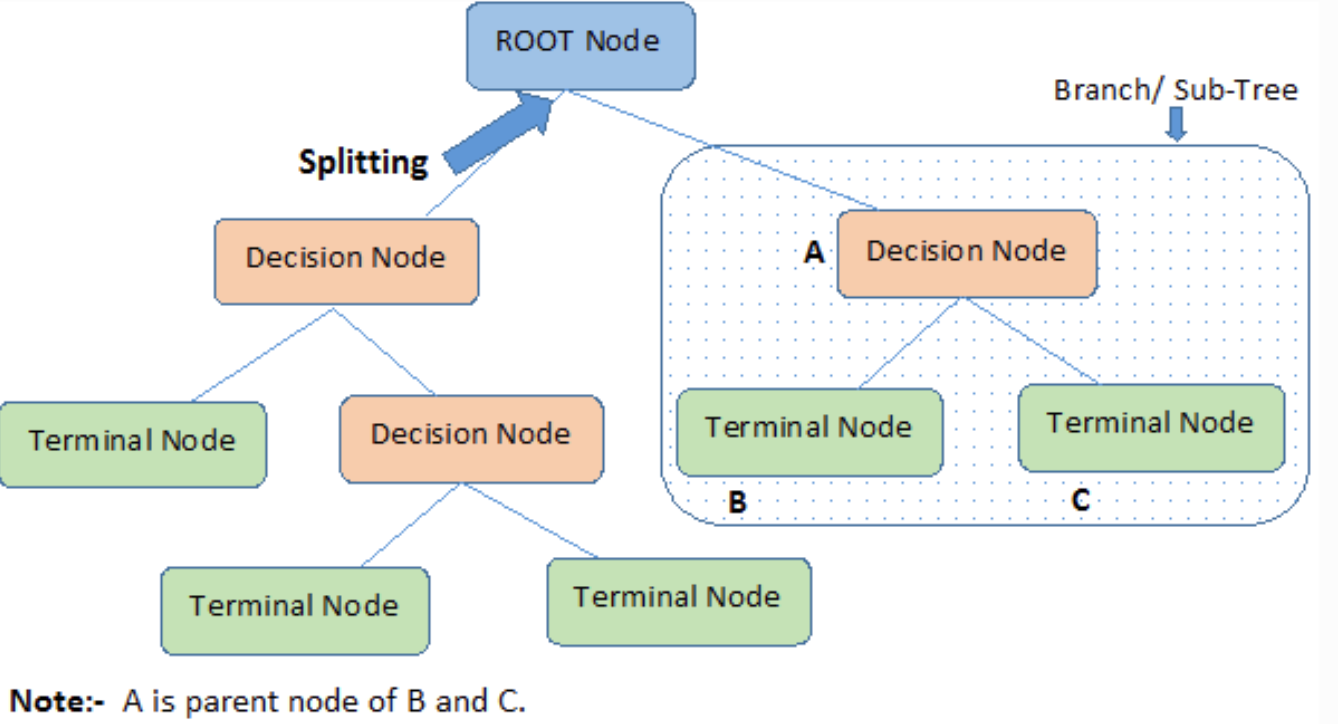
- The internal node denotes a test on an attribute.
- Each branch represents an outcome of the test.
- Each leaf node (terminal node) holds a class label.
-
Here is a figure (source)](https://python.plainenglish.io/decision-trees-easy-intuitive-way-with-python-23131eaad311) that illustrates an example decision tree with the thought process behind deciding to play tennis:
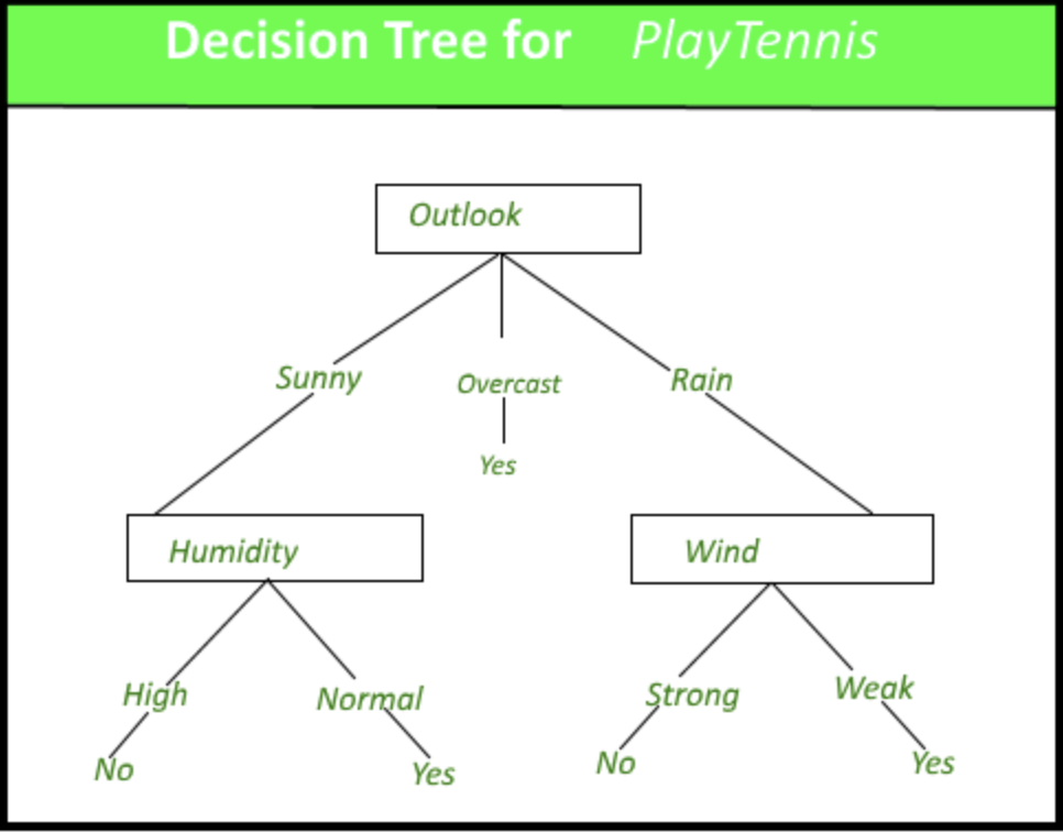
- The objective of a Decision Tree is to create a training model that can to predict the class of the target variable by learning simple decision rules inferred from prior data (training data).
- Pros:
- Interpretability is high due to the intuitive nature of a tree.
- Cons:
- Decision trees are susceptible to overfitting (random forests are a great way to fix this issue).
- Small changes in data can lead to large structural changes on the tree.
- Use case:
- When you want to be able to lay out all the possible outcomes of a problem and work on challenging each option.
Model Ensembles
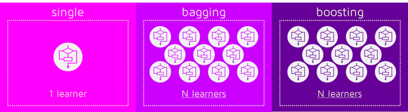
Bagging and Boosting
- Bagging and boosting are two popular ensemble learning techniques used in machine learning to improve the performance of predictive models by combining multiple weaker models. In other words, they combine multiple models to produce a more stable and accurate final model compared to a single classifier. They aim to decrease the bias and variance of a model (with the end goal of having low bias and modest variance to model the nuances of the training data, while not underfitting/overfitting it). While they have similar goals, they differ in their approach and how they create the ensemble.
- Ensemble learning is a powerful approach that combines multiple models to improve the predictive performance of machine learning algorithms. By leveraging the diversity of these models, ensemble learning helps mitigate the issues of bias, variance, and noise commonly encountered in individual models. It achieves this by training a set of classifiers or experts and allowing them to vote or contribute to the final prediction or classification.
Bootstrapping
- Before diving into the specifics of bagging and boosting, let’s first understand bootstrapping. Bootstrapping is a sampling technique that involves creating subsets of observations from the original dataset with replacement.
- Each subset has the same size as the original dataset, and the random sampling allows us to better understand the bias and variance within the dataset. It helps estimate the mean and standard deviation by resampling from the dataset.
Bagging
- Bagging, short for Bootstrap Aggregation, is a straightforward yet powerful ensemble method. It applies the bootstrap procedure to high-variance machine learning algorithms, typically decision trees. The idea behind bagging is to combine the results of multiple models, such as decision trees, to obtain a more generalized and robust prediction. It creates subsets (bags) from the original dataset using random sampling with replacement, and each subset is used to train a base model or weak model independently. These models run in parallel and are independent of each other.
- The final prediction is determined by combining the predictions from all the models, often through averaging or majority voting.
Boosting
- Boosting is a sequential process where each subsequent model attempts to correct the errors made by the previous model. Unlike bagging, boosting involves training learners sequentially, with early learners fitting simple models to the data and subsequent learners analyzing the data for errors. The goal is to solve for net error from the prior model by adjusting the weights assigned to each data point. Boosting assigns higher weights to misclassified data points, so subsequent learners focus more on these difficult cases.
- Through this iterative process, boosting aims to convert a collection of weak learners into a stronger and more accurate model. The final model, often referred to as a strong learner, is a weighted combination of all the models.
Bagging vs. Boosting
- Bagging and Boosting are both ensemble learning techniques used to improve the performance of machine learning models. However, they differ in their approach and objectives. Here are the key differences between Bagging and Boosting:
- Data Sampling:
- Bagging: In Bagging (short for Bootstrap Aggregating), multiple training datasets are created by randomly sampling from the original dataset with replacement. Each dataset is of the same size as the original dataset.
- Boosting: In Boosting, the training datasets are also created by random sampling with replacement. However, each new dataset gives more weight to the instances that were misclassified by previous models. This allows subsequent models to focus more on difficult cases.
- Model Independence:
- Bagging: In Bagging, each model is built independently of the others. They are trained on different subsets of the data and can be constructed in parallel.
- Boosting: In Boosting, models are built sequentially. Each new model is influenced by the performance of previously built models. Misclassified instances are given higher weights, and subsequent models try to correct those errors.
- Weighting of Models:
- Bagging: In Bagging, all models have equal weight when making predictions. The final prediction is often obtained by averaging the predictions of all models or using majority voting.
- Boosting: In Boosting, models are weighted based on their performance. Models with better classification results are given higher weights. The final prediction is obtained by combining the weighted predictions of all models.
- Objective:
- Bagging: Bagging aims to reduce the variance of a single model. It helps to improve stability and reduce overfitting by combining multiple models trained on different subsets of the data.
- Boosting: Boosting aims to reduce the bias of a single model. It focuses on difficult instances and tries to correct the model’s mistakes by giving more weight to misclassified instances. Boosting can improve the overall accuracy of the model but may be more prone to overfitting.
- Examples:
- Bagging: Random Forest is an extension of Bagging that uses decision trees as base models and combines their predictions to make final predictions.
- Boosting: Gradient Boosting is a popular Boosting algorithm that sequentially adds decision trees to the model, with each new tree correcting the mistakes of the previous ones.
- The image below (source) is an illustrated example of bagging and boosting.
Random Forests
- A random forest is a robust ML algorithm that relies on having an ensemble of different models and making them vote for the prediction.
- An essential feature of random forest is to encourage diversity in the models; that way, we ensure the models have different predictions that will improve their model performance.
- Random forest encourages diversity by using random sampling with a replacement but also changing the root node, which is the first feature in which we split our data.
-
The results are a set of decision trees with different root nodes taken from similar (not equal) datasets, and each has a vote in the prediction of the model.
- Pros:
- Less prone to overfitting compared to decision trees.
- Cons:
- Interpretability is low compared to decision trees.
- Use case:
- When the model is overfitting and you want better generalization.
Gradient Boosting
- Gradient Boosting is an ensemble machine learning algorithm that combines multiple weak models to create a strong model.
- It is an iterative process where each iteration, a new model is fit to the residual errors made by the previous model, with the goal of decreasing the overall prediction error.
- The algorithm works as follows:
- Initialize the model with a weak learner, typically a decision tree with a single split.
- Compute the negative gradient of the loss function with respect to the current prediction.
- Fit a new model to the negative gradient.
- Update the prediction by adding the prediction from the new model.
- Repeat steps 2-4 for a specified number of iterations, or until a stopping criterion is met.
- Combine the predictions from all models to get the final prediction.
XGBoost
- XGBoost algorithm is a gradient boosting algorithm that is highly efficient and scalable.
- Here’s a high-level overview of the XGBoost algorithm:
- Initialize the model with a weak learner, usually a decision tree stump (a decision tree with a single split)
- Compute the negative gradient of the loss function with respect to the current prediction
- Fit a decision tree to the negative gradient to make a new prediction
- Add the prediction from this tree to the current prediction
- Repeat steps 2-4 for a specified number of trees, or until a stopping criterion is met
- Combine the predictions from all trees to get the final prediction
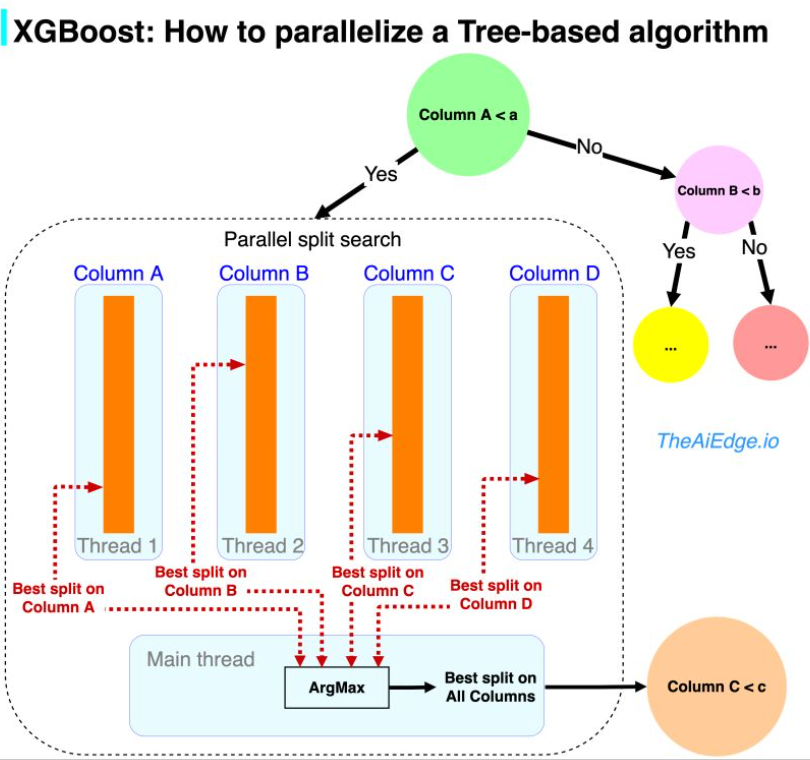
- The following figure summarizes parallelizing XGBoost (source).
- The content below is taken from Damien Benveniste’s LinkedIn post linked here
- But why XGBoost became so popular? There are 2 aspects that made the success of XGBoost back in 2014.
- The first one is the regularized learning objective that allows for better pruning of the trees.
- The second one, is the ability to distribute the Gradient Boosting learning process across multiple threads or machines, allowing it to handle larger scales of data. Boosting algorithms have been known to perform very well on most large data sets, but the iterative process of boosting makes those painfully slow!
- How do you parallelize a boosting algorithm then? In the case of Random Forest, it is easy, you just distribute the data across threads, build independent trees there, and average the resulting tree predictions. In the case of an iterative process like boosting, you need to parallelize the tree building itself. It all comes down to how you find an optimal split in a tree: for each feature, sort the data and linearly scan the feature to find the best split. If you have N samples and M features, it is O(NM log(N)) time complexity at each node. In pseudo-code:
best_split = None
for feature in features:
     for sample in sorted samples:
   if split is better than best_split:
          best_split = f(feature, sample)
- So you can parallelize split search by scanning each feature independently and reduce the resulting splits to the optimal one.
- XGBoost is not the first attempt to parallelize GBM, but they used a series of tricks that made it very efficient:
- First, all the columns are pre-sorted while keeping a pointer to the original index of the entry. This removes the need to sort the feature at every search.
- They used a Compressed Column Format for a more efficient distribution of the data.
- They used a cache-aware prefetching algorithm to minimize the non-contiguous memory access that results from the pre-sorting step.
- Not directly about parallelization, but they came out with an approximated split search algorithm that speeds the tree building further.
-
As of today, you can train XGBoost across cores on the same machine, but also on AWS YARN, Kubernetes, Spark, and GPU and you can use Dask or Ray to do it (https://lnkd.in/dtQTfu62).
- One thing to look out for is that there is a limit to how much XGBoost can be parallelized. With too many threads, the data communication between threads becomes a bottleneck and the training speed plateaus. Here is a example explaining that effect: https://lnkd.in/d9SEcQuV.

<!–Clustering in Machine Learning: Latent Dirichlet Allocation and K-Means
- Clustering is a type of unsupervised learning method in machine learning, as it involves grouping unlabeled data based on their underlying patterns. This article will delve into two popular clustering algorithms: Latent Dirichlet Allocation (LDA) and K-Means.
What is K-Means Clustering?
- K-Means is a centroid-based clustering method, meaning it clusters the data into k different groups by trying to minimize the distance between data points in the same group, often measured by Euclidean distance. The center of each group (the centroid) is calculated as the mean of all the data points in the cluster.
- Here’s how the algorithm works:
- Select k initial centroids, where k is a user-defined number of clusters.
- Assign each data point to the nearest centroid. These clusters will form the initial clusters.
- Recalculate the centroid (mean) of each cluster.
- Repeat steps 2 and 3 until the centroids don’t change significantly, or a maximum number of iterations is reached.
- K-Means is a simple yet powerful algorithm, but it has its drawbacks. The algorithm’s performance can be greatly affected by the choice of initial centroids and the value of k. Additionally, it works best on datasets where clusters are spherical and roughly the same size.
What is Latent Dirichlet Allocation (LDA)?
- Latent Dirichlet Allocation (LDA) is a generative statistical model widely used for topic modeling in natural language processing. Rather than clustering based on distances, LDA assumes that each document in a corpus is a mixture of a certain number of topics, and each word in the document is attributable to one of the document’s topics.
- In LDA:
- You specify the number of topics (k) you believe exist in your corpus.
- The algorithm assigns every word in every document to a temporary topic (initially, this assignment is random).
- For each document, the algorithm goes through each word, and for each topic, calculates:
- How often the topic occurs in the document, and
- How often the word occurs with the topic throughout the corpus.
- Based on these calculations, the algorithm reassigns the word to a new topic.
- Steps 3 and 4 are repeated a large number of times, and the algorithm ultimately provides a steady state where the document topic and word topic assignments are considered optimal.
- LDA’s major advantage is its ability to uncover hidden thematic structure in the corpus. However, its interpretability relies heavily on the quality of the text preprocessing and the choice of the number of topics, which often requires domain knowledge.
Machine Learning or Deep Learning?
- Both K-means and LDA are traditional machine learning algorithms. They rely on explicit programming and feature engineering, whereas deep learning algorithms automatically discover the features to be used for learning through the learning process by building high-level features from data.
- Nevertheless, they remain essential tools in the data scientist’s arsenal. The choice between machine learning or deep learning methods will depend on the problem at hand, the nature of the data available, and the computational resources at your disposal.
Hidden Markov Model (HMM) in Machine Learning
- Hidden Markov Models (HMMs) are statistical models that have been widely applied in various fields of study, including finance, genomics, and most notably in natural language processing and speech recognition systems.
What is a Hidden Markov Model?
- A Hidden Markov Model is a statistical model where the system being modeled is assumed to be a Markov process — i.e., a random process where the future states depend only on the current state and not on the sequence of events that preceded it — with hidden states.
-
In an HMM, we deal with two types of sequences:
- An observable sequence (also known as emission sequence)
- A hidden sequence, which corresponds to the hidden states that generate the observable sequence
- The term “hidden” in HMM refers to the fact that while the output states (observable sequence) are visible to an observer, the sequence of states that led to those outputs (hidden sequence) is unknown or hidden.
Key Components of an HMM
- A Hidden Markov Model is characterized by the following components:
-
States: These are the hidden states in the model. They cannot be directly observed, but they can be inferred from the observable states.
-
Observations: These are the output states which are directly visible.
-
Transition Probabilities: These are the probabilities of transitioning from one hidden state to another.
-
Emission Probabilities: These are the probabilities of an observable state being generated from a hidden state.
-
Initial State Probabilities: These are the probabilities of starting in each hidden state.
Applications of HMMs in NLP
- In the field of Natural Language Processing, HMMs have been extensively used, especially for tasks like Part-of-Speech (POS) tagging, Named Entity Recognition (NER), and even in speech recognition and machine translation systems. For instance, in POS tagging, the hidden states could represent the parts of speech, while the visible states could represent the words in sentences.
Pros and Cons of HMMs
- HMMs are beneficial due to their simplicity, interpretability, and their effectiveness in dealing with temporal data. However, they make some strong assumptions, like the Markov assumption and the assumption of independence among observable states given the hidden states, which may not hold true in all scenarios. Additionally, HMMs may suffer from issues with scalability and can struggle to model complex, long-distance dependencies in the data.
- Despite these limitations, HMMs remain a valuable tool in the machine learning toolbox and serve as a foundation for more complex models in sequence prediction tasks. –>
Summary
- Linear Regression
- Definition: Linear regression is a supervised learning algorithm used for predicting a continuous target variable based on one or more input features.
- Pros: Simple and interpretable, fast training and prediction, works well with linear relationships.
- Cons: Assumes linear relationships, sensitive to outliers, may not capture complex patterns.
- Decision Trees
- Definition: Decision trees are hierarchical structures that make decisions based on a sequence of rules and conditions, leading to a final prediction.
- Pros: Easy to understand and interpret, handles both numerical and categorical data, can capture non-linear relationships.
- Cons: Prone to overfitting, can be unstable and sensitive to small changes in data.
- Random Forest
- Definition: Random forest is an ensemble learning method that combines multiple decision trees to make predictions.
- Pros: Robust and handles high-dimensional data, reduces overfitting through ensemble learning, provides feature importance.
- Cons: Requires more computational resources, lack of interpretability for individual trees.
- Support Vector Machines (SVM)
- Definition: Support Vector Machines is a binary classification algorithm that finds an optimal hyperplane to separate data into different classes.
- Pros: Effective in high-dimensional spaces, works well with both linear and non-linear data, handles outliers well.
- Cons: Can be sensitive to the choice of kernel function and parameters, computationally expensive for large datasets.
- Naive Bayes
- Definition: Naive Bayes is a probabilistic classifier that applies Bayes’ theorem with the assumption of independence between features.
- Pros: Simple and fast, works well with high-dimensional data, performs well with categorical features.
- Cons: Assumes independence between features, may not capture complex relationships.
- Neural Networks
- Definition: Neural networks are a set of interconnected nodes or “neurons” organized in layers, capable of learning complex patterns from data.
- Pros: Powerful and flexible, can learn complex patterns, works well with large datasets, can handle various data types.
- Cons: Requires large amounts of data for training, computationally intensive, prone to overfitting if not properly regularized.
- K-Nearest Neighbors (kNN)
- Definition: k-Nearest Neighbors is a non-parametric algorithm that makes predictions based on the majority vote of its k nearest neighbors.
- Pros: Simple and easy to understand, no training phase, works well with small datasets and non-linear data.
- Cons: Computationally expensive during prediction, sensitive to irrelevant features, doesn’t provide explicit model representation.
- Gradient Boosting
- Definition: Gradient Boosting is an ensemble method that combines weak learners (typically decision trees) to create a strong predictive model.
- Pros: Produces highly accurate models, handles different types of data, handles missing values well, provides feature importance.
- Cons: Can be prone to overfitting if not properly tuned, computationally expensive.
Comparative Analysis: Linear Regression, Logistic Regression, Support Vector Machines, k-Nearest Neighbors, and k-Means
- Here’s a detailed comparative analysis of Linear Regression, Logistic Regression, Support Vector Machines, k-Nearest Neighbors, and k-Means, ighlighting their strengths, limitations, and typical use cases.
| Aspect | Linear Regression | Logistic Regression | SVM (Support Vector Machine) | k-Nearest Neighbors (kNN) | k-Means |
|---|---|---|---|---|---|
| Type of Algorithm | Regression | Classification (Binary/Multiclass) | Classification and Regression | Classification and Regression | Clustering |
| Purpose | Predict continuous values | Predict probability of categorical outcomes | Classify or predict by finding optimal decision boundary | Predict or classify based on nearest neighbors | Cluster unlabeled data into groups |
| Mathematical Model | Minimizes the sum of squared errors (OLS) | Uses the logistic function to model probabilities | Maximizes margin between data points and decision boundary | Distance-based similarity (e.g., Euclidean distance) | Minimizes within-cluster variance |
| Training Complexity | Low; O(n) | Low; O(n) | Moderate to High; depends on kernel type (linear vs. non-linear) | Low for small data; High for large datasets | Moderate; depends on iterations and clusters |
| Scalability | Scales well for large datasets | Scales well for large datasets | Can struggle with very large datasets without kernel approximation | Poor for high-dimensional data or large datasets | Good; scales with the number of clusters |
| Key Parameters | Coefficients (weights) | Coefficients (weights) | Regularization parameter (C), kernel type (e.g., linear, RBF) | Number of neighbors (k), distance metric | Number of clusters (k), initialization method |
| Handling Non-linearity | Poor, assumes linear relationships | Poor, though some non-linear relationships can be modeled with feature engineering | Excellent with kernel functions (e.g., RBF, polynomial) | Poor without feature engineering | Assumes clusters are roughly spherical |
| Advantages | - Simple to implement - Easy to interpret |
- Interpretable - Handles probabilities - Effective for binary classification |
- Effective in high dimensions - Handles non-linear boundaries well |
- Simple and intuitive - No training required |
- Simple - Works on unlabeled data |
| Disadvantages | - Assumes linear relationship - Sensitive to outliers |
- Assumes linear decision boundary - Limited to classification |
- Computationally expensive - Sensitive to kernel and C parameters |
- Sensitive to noise - High memory usage |
- Sensitive to initialization - Prone to local minima |
| Output | Continuous variable (real number) | Probability values (0 to 1); classification labels | Decision boundary, support vectors, classification labels | Class label for classification Value for regression |
Cluster centroids and cluster assignments |
| Typical Applications | - Predicting house prices - Stock market analysis |
- Email spam detection - Medical diagnosis |
- Face recognition - Text classification |
- Recommendation systems - Handwriting recognition |
- Customer segmentation - Image compression |
| Handling Outliers | Sensitive to outliers | Sensitive to outliers | Can be robust (depends on kernel and margin settings) | Highly sensitive to outliers | Sensitive to noise and outliers |
| Assumptions | - Linear relationship - Homoscedasticity - Independence of errors |
Linearly separable classes (in basic form) | No assumption of linearity; relies on kernel function | No specific assumption about data distribution | Assumes clusterable structure |
| Evaluation Metrics | Mean Squared Error (MSE), R-squared | Accuracy, Precision, Recall, F1-Score | Accuracy, Precision, Recall, F1-Score | Accuracy, Precision, Recall, F1-Score | Inertia (within-cluster sum of squares) |
References
- IBM tech blog: What is logistic regression?
- Google Crash Course
- Towards Data Science
- Analytics Vidhya
- Science Direct
- SciKit Learn
- KD Nuggets
- Geeks for Geeks
- KD Nuggets Trees
- Edureka
Citation
If you found our work useful, please cite it as:
@article{Chadha2020DistilledMLAlgorithmsCompAnalysis,
  title   = {ML Algorithms Comparative Analysis},
  author  = {Chadha, Aman},
  journal = {Distilled AI},
  year    = {2020},
  note    = {\url{https://aman.ai}}
}