Primers • Loss Functions
- Overview
- Multi-Class Classification
- Multi-Label Classification
- Classification
- Regression Loss Functions
- Ranking Loss
- Contrastive Loss
- Losses in Deep Learning-based Reinforcement Learning
- Further Reading
- References
- Citation
Overview
-
Loss functions, also referred to as cost or error functions, are a foundational component of machine learning systems. They quantify the discrepancy between a model’s predicted outputs and the corresponding ground truth targets. By providing a scalar measure of prediction quality, loss functions act as the primary feedback signal used by optimization algorithms, such as gradient descent, to iteratively update model parameters. In general, larger discrepancies between predictions and targets result in higher loss values, while more accurate predictions yield lower loss values. A comprehensive treatment of loss minimization in supervised learning can be found in Pattern Recognition and Machine Learning by Bishop (2006) and The Elements of Statistical Learning by Hastie et al. (2009).
-
Different machine learning tasks impose different structural assumptions on the output space and the underlying data-generating process. As a consequence, no single loss function is universally optimal. Instead, specific loss functions are designed to align with the statistical properties and optimization objectives of particular problem settings, such as classification, regression, ranking, or reinforcement learning. For example, classification losses are typically derived from probabilistic likelihoods over discrete labels, while regression losses often assume continuous-valued targets with additive noise. A general discussion of task-dependent objective functions is provided in Deep Learning by Goodfellow et al. (2016).
-
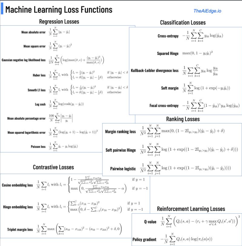
The following figure (source) summarizes several commonly used loss functions and their typical application domains.
-
For readers seeking a refresher on activation functions commonly paired with these loss functions, such as the sigmoid and softmax functions, refer to the Activations primer. These activation functions play a critical role in mapping model outputs to valid probability distributions, which is a prerequisite for losses such as cross-entropy. A classical reference on softmax and logistic activations in probabilistic models is A Tutorial on the Softmax Function by Bridle (1990).
-
In this article, we systematically examine the major categories of machine learning tasks and subsequently analyze the loss functions most commonly employed to optimize models within each category. The discussion spans classification, regression, ranking, and reinforcement learning, with an emphasis on the theoretical motivation, mathematical formulation, and practical implications of each loss function.
Loss Functions vs. Utility Functions
-
Loss functions and utility functions arise from different theoretical frameworks and encode fundamentally different optimization objectives, even though they are mathematically related. The distinction is not merely semantic; it reflects whether a problem is formulated as error minimization or preference maximization.
-
A loss function is a scalar-valued function that quantifies the discrepancy between a model’s prediction and an observed target. In supervised learning, loss functions are explicitly constructed to be minimized. They are typically derived from statistical assumptions about the data-generating process, such as Gaussian noise for regression or categorical and Bernoulli distributions for classification. Minimizing a loss function corresponds to estimating model parameters that best explain the observed data under these assumptions. This perspective is central to statistical learning theory and is thoroughly developed in Pattern Recognition and Machine Learning by Bishop (2006) and The Elements of Statistical Learning by Hastie et al. (2009).
-
A utility function is a more general concept originating from economics and decision theory. It assigns a real-valued score to outcomes or states of the world, representing how desirable they are to an agent. Utility functions are designed to be maximized rather than minimized and encode preferences, trade-offs, and long-term objectives. Unlike loss functions, utility functions are not necessarily tied to probabilistic modeling assumptions or ground truth labels. Classical foundations of utility theory are presented in Theory of Games and Economic Behavior by von Neumann and Morgenstern (1944).
-
A reward function can be viewed as a specific, operational instance of a utility function. In reinforcement learning, the reward function assigns immediate scalar feedback to state-action transitions, indicating how desirable a particular outcome is at a given time step. The agent’s objective is not to maximize immediate reward alone, but to maximize the expected cumulative reward over a trajectory, which corresponds to maximizing expected utility. This formulation is standard in reinforcement learning and is formalized in Reinforcement Learning: An Introduction by Sutton and Barto (2018).
-
In this sense, reward functions serve as local or incremental utility signals that, when accumulated over time, define the agent’s overall utility. While utility functions in economics are often abstract and global, reward functions are concrete, task-specific, and designed to be optimized through interaction with an environment.
-
From a mathematical perspective, loss functions and utility functions are often related by a simple sign change. Minimizing a loss is equivalent to maximizing a negative utility, and vice versa. However, the distinction in terminology signals the modeling intent: loss functions emphasize prediction error and statistical consistency, while utility functions emphasize goal-directed behavior and preference satisfaction. This distinction is explicitly discussed in Deep Learning by Goodfellow et al. (2016), particularly in the context of supervised learning versus reinforcement learning.
-
In summary, loss functions are used to measure and minimize prediction error in supervised learning, utility functions represent preferences to be maximized in decision-theoretic settings, and reward functions are a particular type of utility function tailored for sequential decision-making in reinforcement learning.
Multi-Class Classification
-
Multi-class classification, often referred to as one-of-many classification, is a supervised learning setting in which each input instance is assumed to belong to exactly one class out of a finite set of \(C\) mutually exclusive classes. This assumption implies that the class labels form a categorical random variable. Canonical examples include handwritten digit recognition, document topic classification, and object recognition, as discussed in Pattern Recognition and Machine Learning by Bishop (2006).
-
In a typical neural network formulation, the model produces \(C\) output logits, which are collected into a score vector \(\mathbf{s} = (s_1, \dots, s_C)\). These logits are then passed through the softmax activation function to obtain a valid probability distribution over classes:
\[p_j = \frac{e^{s_j}}{\sum_{k=1}^{C} e^{s_k}}\]- The softmax function ensures that each predicted probability \(p_j\) lies in the interval \((0,1)\) and that the probabilities sum to one. A detailed discussion of the softmax function and its probabilistic interpretation is provided in Deep Learning by Goodfellow et al. (2016).
-
The ground-truth label for each instance is typically represented as a one-hot encoded target vector \(\mathbf{t}\) of dimension \(C\), where exactly one component is equal to 1, corresponding to the correct class, and all remaining components are 0. This encoding reflects the assumption that the true data-generating distribution assigns probability 1 to the correct class and 0 to all others for a given labeled example.
-
Conceptually, multi-class classification is treated as a single unified prediction problem rather than \(C\) independent binary classification problems. The model is trained to assign the highest probability mass to the correct class while simultaneously suppressing probabilities assigned to incorrect classes.
-
The most commonly used loss function for multi-class classification is the categorical cross-entropy loss, which arises from the negative log-likelihood of a categorical distribution. For a dataset consisting of \(N\) samples, the categorical cross-entropy loss is defined as:
\[L = -\frac{1}{N} \sum_{i=1}^{N} \sum_{j=1}^{C} t_{ij} \log(p_{ij})\]-
where:
- \(N\) is the total number of samples,
- \(t_{ij}\) denotes the one-hot encoded ground-truth label for sample \(i\) and class \(j\),
- \(p_{ij}\) is the predicted probability for sample \(i\) belonging to class \(j\).
-
-
Because only one entry of \(t_{ij}\) is nonzero for each sample, the loss for a given sample reduces to the negative logarithm of the predicted probability assigned to the correct class. This formulation directly corresponds to maximum likelihood estimation under a categorical distribution, as described in The Elements of Statistical Learning by Hastie et al. (2009).
-
In practice, categorical cross-entropy is almost always implemented together with the softmax activation function in a numerically stable combined form, often referred to as softmax cross-entropy or softmax loss. This combined formulation avoids numerical instability caused by exponentiation and logarithms and is standard in modern deep learning frameworks. A clear exposition of this implementation detail can be found in CS231n: Convolutional Neural Networks for Visual Recognition by Stanford University.
Multi-Label Classification
-
In multi-label classification, each input instance may simultaneously belong to multiple classes. This setting contrasts with multi-class classification, where class membership is mutually exclusive and exactly one label is correct per instance. Common examples of multi-label classification include image tagging, where an image may contain multiple objects, document categorization with overlapping topics, and music genre classification, as discussed in A Survey on Multi-Label Classification by Zhang and Zhou (2014).
-
As in multi-class classification, the model typically produces \(C\) output neurons, one for each class. However, in the multi-label setting, these outputs are interpreted independently rather than as components of a single categorical distribution. Consequently, the target vector \(\mathbf{t}\) is a multi-hot vector of dimension \(C\), in which multiple entries may be equal to 1, indicating that the corresponding classes are present for the given instance, while the remaining entries are 0.
-
Because class memberships are not mutually exclusive, the softmax activation function is generally inappropriate for multi-label classification. Instead, each output neuron is usually passed through a sigmoid activation function, producing \(C\) independent probabilities, each lying in the interval \((0,1)\). Each probability represents the model’s confidence that the corresponding class is present. This modeling assumption aligns with treating each class as an independent Bernoulli random variable conditioned on the input. A probabilistic treatment of this formulation is provided in Pattern Recognition and Machine Learning by Bishop (2006).
-
From an optimization perspective, multi-label classification is typically formulated as \(C\) independent binary classification problems. Each output neuron contributes a binary prediction, and the overall loss is computed by aggregating the losses across all classes. The most commonly used loss function in this setting is the binary cross-entropy loss, applied independently to each class and then averaged or summed across classes and samples. This approach is widely adopted in deep learning systems, as described in Deep Learning by Goodfellow et al. (2016).
-
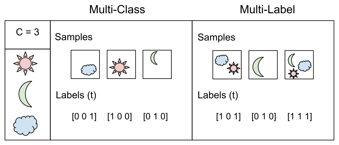
The image above (source) visually highlights the conceptual difference between multi-class and multi-label classification. In multi-class classification, exactly one class is active per sample, whereas in multi-label classification, multiple classes may be active simultaneously. This distinction has important implications for both the choice of activation functions and the choice of loss functions.
-
In summary, the defining characteristics of multi-label classification are the absence of mutual exclusivity among classes, the use of sigmoid activations rather than softmax, and the adoption of binary cross-entropy as the primary loss function. These design choices ensure that the learning objective properly reflects the underlying structure of the task and the semantics of the labels.
Classification
Cross-Entropy Loss
-
Cross-entropy loss is one of the most widely used objective functions for training classification models. It measures the discrepancy between the true label distribution and the probability distribution predicted by the model. The predicted probabilities are typically obtained from a sigmoid activation function in binary classification or a softmax activation function in multi-class classification. A foundational discussion of cross-entropy in statistical learning can be found in Pattern Recognition and Machine Learning by Bishop (2006).
-
Intuitively, cross-entropy quantifies how “surprised” the model is by the true labels given its predicted probability distribution. When the predicted probability assigned to the correct class is high, the loss is low; when this probability is low, the loss increases sharply. In the ideal case of a perfect classifier that assigns probability 1 to the correct class, the cross-entropy loss evaluates to 0.
-
For binary classification problems, the binary cross-entropy loss is used. For multi-class classification problems with mutually exclusive classes, the categorical cross-entropy loss is employed. Both are special cases of the same underlying principle: minimizing the negative log-likelihood of the observed labels under the model’s predicted distribution. This connection is discussed in detail in The Elements of Statistical Learning by Hastie et al. (2009).
-
More formally, cross-entropy loss computes the error between the model’s predicted probability distribution and the true class labels, which are represented as one-hot encoded vectors in the multi-class case or binary indicators in the binary case. The predicted probabilities are differentiable with respect to the model parameters, enabling gradient-based optimization.
While cross-entropy seeks to maximize the likelihood of the predicted probability distribution matching the target or label distribution, learning algorithms are conventionally framed as minimization problems. As a result, the objective is expressed as the negative log-likelihood, introducing a negative sign in front of the summation.
-
The binary cross-entropy loss for a two-class problem (where the number of classes \(M = 2\)) is given by:
\[\text {Cross-Entropy Loss}=-(y \log(p) +(1-y)\log(1-p))\]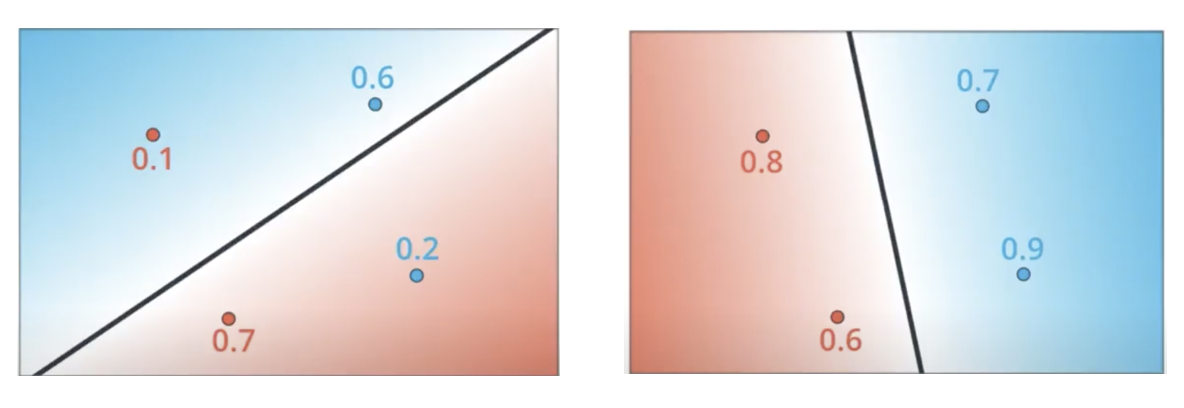
-
where:
- \(M\) is the number of classes,
- \(y\) is the ground-truth label, taking values in \({0,1}\),
- \(p\) is the predicted probability of the positive class.
-
-
In some literature, the predicted probability is denoted by \(\hat{y}\), yielding the equivalent expression:
\[\text {Cross-Entropy Loss}=-\left(y_{i} \log \left(\hat{y}_{i}\right)+\left(1-y_{i}\right) \log \left(1-\hat{y}_{i}\right)\right)\] -
For multi-class classification problems where the number of classes \(M > 2\), the categorical cross-entropy loss is defined as:
\[\text {Cross-Entropy Loss}=-\sum_{c=1}^{M} y_{o, c} \log \left(p_{o, c}\right)\]-
where:
- \(M\) is the number of classes,
- \(y_{o, c}\) is the one-hot encoded ground-truth indicator that equals 1 if class \(c\) is the correct label for observation \(o\) and 0 otherwise,
- \(p_{o, c}\) is the predicted probability that observation \(o\) belongs to class \(c\).
-
-
Because only one component of the one-hot vector \(y_{o}\) is nonzero, the categorical cross-entropy loss for a single observation reduces to the negative logarithm of the predicted probability assigned to the correct class. This property explains why cross-entropy strongly penalizes confident but incorrect predictions.
-
During training, the gradients of the cross-entropy loss with respect to the model parameters encourage the predicted probability of the correct class to increase while decreasing the probabilities of incorrect classes. Importantly, the loss is computed using the pre-argmax outputs of the model, since the argmax operation is non-differentiable and therefore unsuitable for gradient-based optimization.
-
A clear and intuitive introduction to the information-theoretic motivation behind cross-entropy, including its relationship to entropy and surprise, is provided in Chris Olah’s blog post Visual Information Theory.
Equivalence between Cross-Entropy Loss, Maximum Likelihood Estimation, and Negative Log Likelihood (NLL)
-
Cross-entropy minimization, maximum likelihood estimation (MLE), and negative log-likelihood (NLL) minimization are mathematically equivalent objectives expressed through different conceptual frameworks. Cross-entropy arises from information theory, MLE from statistical inference, and NLL from optimization-oriented reformulations of likelihood-based learning. Despite their differing interpretations, they lead to identical parameter updates when applied to probabilistic classification models. This equivalence is a cornerstone of modern supervised learning and is discussed extensively in Pattern Recognition and Machine Learning by Bishop (2006) and The Elements of Statistical Learning by Hastie et al. (2009).
-
In supervised learning, it is assumed that labels \(y\) are generated according to an unknown conditional data distribution \(p_{\text{data}}(y \mid x)\). A parametric model with parameters \(\theta\) defines a conditional distribution \(p_\theta(y \mid x)\) intended to approximate this unknown distribution. The objective of learning is to select parameters \(\theta\) such that the model assigns high probability to the observed labels given the corresponding inputs.
-
Under the maximum likelihood estimation framework, this objective is formalized as maximizing the likelihood of the observed training data:
- Taking the logarithm of the likelihood yields the log-likelihood function:
- Since optimization algorithms in machine learning are conventionally framed as minimization problems, the negative log-likelihood is minimized instead:
- This expression is precisely the empirical cross-entropy between the true data distribution and the model’s predicted distribution. In classification tasks, the true distribution is represented using one-hot encoded labels. When the model outputs probabilities via a sigmoid function (binary classification) or a softmax function (multi-class classification), the cross-entropy loss can be written as:
- Because the one-hot encoded target vector has exactly one nonzero entry, this expression simplifies for each training example to:
-
Consequently, minimizing cross-entropy is equivalent to maximizing the likelihood assigned by the model to the correct class label for each input. This equivalence underpins the widespread use of cross-entropy loss in probabilistic classifiers such as logistic regression and softmax regression, as discussed in Deep Learning by Goodfellow et al. (2016).
-
From an information-theoretic perspective, the cross-entropy between the true data distribution \(p_{\text{data}}\) and the model distribution \(p_\theta\) can be decomposed as:
-
The entropy term \(H(p_{\text{data}})\) depends only on the data-generating process and is independent of the model parameters. As a result, minimizing cross-entropy with respect to \(\theta\) is equivalent to minimizing the Kullback–Leibler divergence between the true data distribution and the model distribution. This decomposition is a standard result in information theory and is covered in Elements of Information Theory by Cover and Thomas (2006).
-
In summary, training a classifier using cross-entropy loss is mathematically identical to performing maximum likelihood estimation under the assumed probabilistic model. The differences between cross-entropy, NLL, and MLE lie solely in interpretation and terminology rather than in the underlying optimization objective.
Binary cross-entropy loss
-
In supervised machine learning, binary classification refers to the task of assigning each input instance to one of two possible classes. The target variable is typically modeled as a Bernoulli random variable. A common neural network formulation uses a single output neuron, whose raw output (logit) is passed through a sigmoid activation function to produce a probability value in the interval \([0,1]\). A prediction threshold, often set to 0.5, is then used at inference time to map probabilities to class labels, although this threshold may be adjusted depending on the application and class imbalance considerations. A probabilistic treatment of binary classification is provided in Pattern Recognition and Machine Learning by Bishop (2006).
-
Binary cross-entropy loss, also referred to as sigmoid cross-entropy loss or log loss, is derived from the negative log-likelihood of a Bernoulli distribution. It measures the discrepancy between the true binary labels and the predicted probabilities output by the sigmoid function. This loss function is the canonical choice for binary classification models trained using gradient-based optimization. A clear derivation is presented in Deep Learning by Goodfellow et al. (2016).
-
Conceptually, binary cross-entropy penalizes confident but incorrect predictions much more strongly than uncertain ones. Predictions that assign high probability to the incorrect class incur a large loss, while predictions that assign high probability to the correct class incur a small loss. This property leads to well-behaved gradients and stable learning dynamics in practice.
-
Binary cross-entropy loss can be viewed as the composition of a sigmoid activation function with a cross-entropy objective, as illustrated below (source).

-
Formally, for a dataset consisting of \(N\) samples, the binary cross-entropy loss is defined as:
\[L = -\frac{1}{N} \sum \left[y \log(\hat{y}) + (1 - y)\log(1 - \hat{y})\right]\]-
where:
- \(y \in {0,1}\) denotes the ground-truth label,
- \(\hat{y}\) is the predicted probability output by the sigmoid function,
- \(N\) is the total number of samples.
-
-
This formulation corresponds exactly to the negative log-likelihood of the Bernoulli distribution under the model’s predicted probabilities. Minimizing this loss is therefore equivalent to performing maximum likelihood estimation for a Bernoulli observation model, as discussed in The Elements of Statistical Learning by Hastie et al. (2009).
-
Typical application domains for binary classification and binary cross-entropy loss include:
- medical diagnostics, such as determining whether a patient has a particular disease;
- industrial quality control, where items are classified as defective or non-defective;
- information retrieval and recommendation systems, where a model predicts whether a document, item, or result is relevant to a given query.
-
In practice, most deep learning libraries provide a numerically stable combined implementation of the sigmoid function and binary cross-entropy loss. This avoids numerical issues arising from computing logarithms of values close to 0 or 1 and improves training stability. An example of such an implementation is discussed in CS231n: Linear Classification.
Focal Loss
-
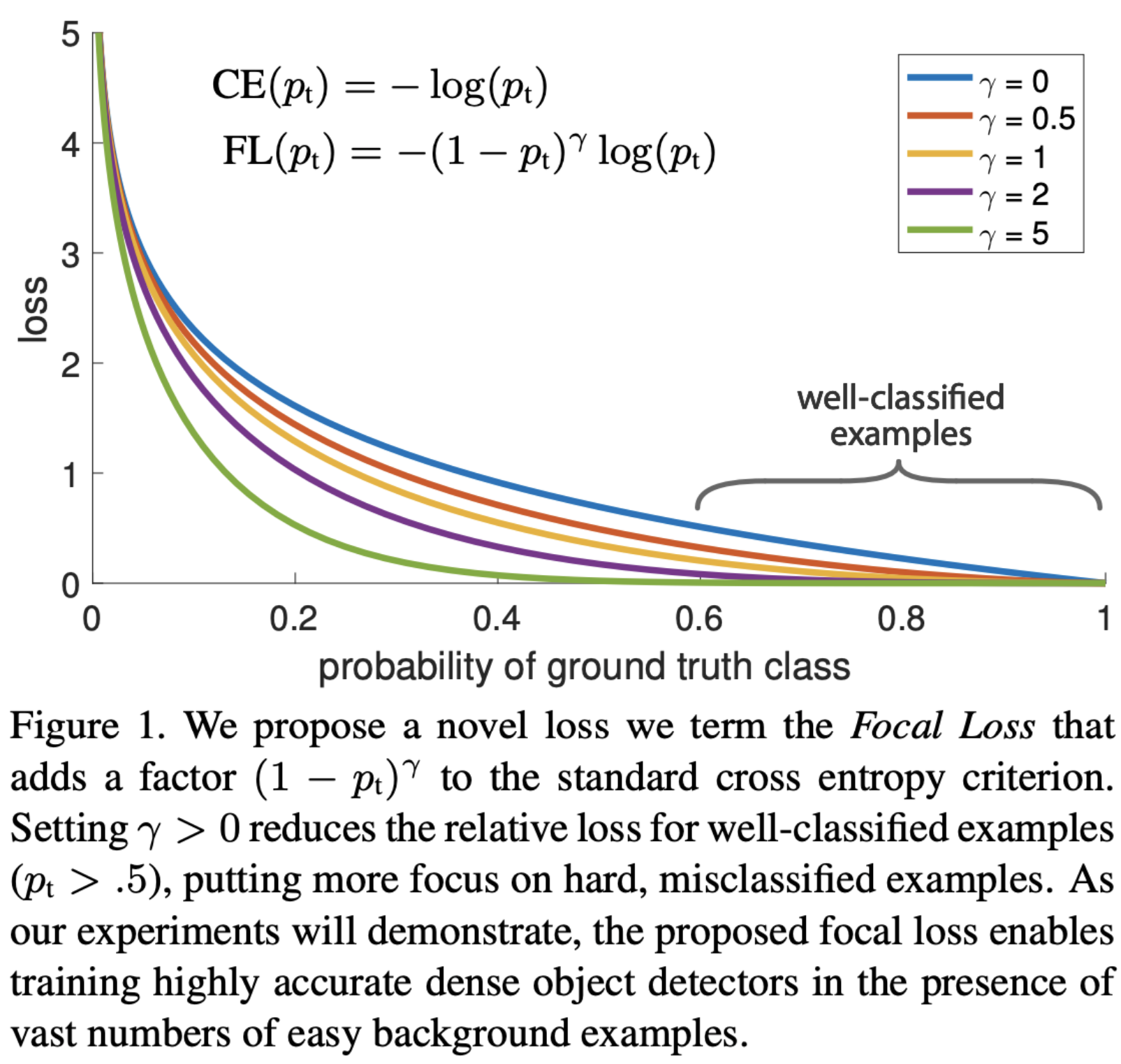
Focal Loss was introduced by Facebook AI Research in Focal Loss for Dense Object Detection by Lin et al. (2017) to address the problem of severe class imbalance, particularly in dense object detection tasks such as those encountered in one-stage detectors. In such settings, the vast majority of training examples are easy negatives, which can dominate the loss and hinder effective learning.
-
The central idea behind Focal Loss is to modify the standard cross-entropy loss by down-weighting well-classified (easy) examples and focusing training on hard, misclassified examples. This is achieved by introducing a modulating factor that dynamically scales the contribution of each training example based on the model’s confidence in its prediction.
-
Focal Loss is most commonly applied in classification settings where class imbalance is pronounced, including object detection, face detection, and certain medical imaging tasks. It has also been adopted more broadly in classification problems where robustness to class imbalance is desired. A detailed empirical evaluation is provided in the original paper by Lin et al. (2017).
-
Formally, Focal Loss is defined as a modified version of cross-entropy loss:
-
where:
- \(p_t\) denotes the model’s predicted probability for the true class,
- \(\gamma \geq 0\) is the focusing parameter that controls the strength of the modulation.
-
When \(\gamma = 0\), the Focal Loss reduces exactly to the standard cross-entropy loss. As \(\gamma\) increases, the loss assigned to well-classified examples (those with large \(p_t\)) is progressively down-weighted, while the loss for poorly classified examples remains comparatively large. This mechanism effectively reallocates learning capacity toward hard examples during training.
-
In practice, Focal Loss is often combined with an additional class-balancing factor \(\alpha\) to explicitly counteract class imbalance by reweighting positive and negative examples. The complete formulation including this factor is described in Focal Loss for Dense Object Detection by Lin et al. (2017).
-
From an optimization perspective, Focal Loss preserves the desirable gradient properties of cross-entropy loss while reducing the influence of overwhelming numbers of easy examples. This results in improved convergence behavior and empirical performance in highly imbalanced classification settings, as demonstrated in large-scale object detection benchmarks.
Categorical Cross Entropy
-
Categorical cross-entropy loss is the standard objective function for multi-class classification problems in which each input instance belongs to exactly one class out of a finite set of mutually exclusive classes. It is derived from the negative log-likelihood of a categorical (multinomial) distribution and measures the discrepancy between the true class distribution and the probability distribution predicted by the model. A formal treatment of this loss in probabilistic classifiers is provided in Pattern Recognition and Machine Learning by Bishop (2006).
-
Categorical cross-entropy is sometimes informally referred to as “softmax loss.” This terminology reflects the fact that, in practice, the loss is almost always used in conjunction with a softmax activation function applied to the model’s output logits. It is important to distinguish between the softmax function itself, which maps logits to a probability distribution, and the cross-entropy loss, which evaluates how well that distribution matches the true labels. The combined operation of softmax followed by cross-entropy is illustrated below (source).
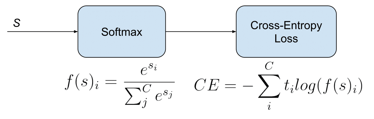
- In this setting, the model outputs a vector of logits \(\mathbf{s} \in \mathbb{R}^C\), which are transformed by the softmax function into class probabilities:
- The ground-truth label is represented as a one-hot encoded vector \(\mathbf{y}\), where exactly one component corresponding to the correct class is equal to 1, and all other components are 0. The categorical cross-entropy loss for a single observation is then given by:
-
Because only the component corresponding to the correct class is nonzero in the one-hot target vector, the loss reduces to the negative logarithm of the predicted probability assigned to the true class. This property explains why categorical cross-entropy strongly penalizes confident but incorrect predictions and encourages the model to concentrate probability mass on the correct class.
-
From a statistical perspective, minimizing categorical cross-entropy is equivalent to performing maximum likelihood estimation under a categorical distribution, assuming the training labels are drawn from the true data-generating distribution. This equivalence is discussed in The Elements of Statistical Learning by Hastie et al. (2009) and Deep Learning by Goodfellow et al. (2016).
-
In modern deep learning libraries, categorical cross-entropy is typically implemented in a numerically stable fused form that combines the softmax operation and the logarithm into a single function. This avoids numerical instability caused by exponentiation and logarithms when probabilities approach 0 or 1 and improves both computational efficiency and training stability. An implementation-oriented discussion can be found in CS231n: Linear Classification.
-
In summary, categorical cross-entropy is the canonical loss function for multi-class classification with mutually exclusive classes. Its probabilistic grounding, favorable optimization properties, and strong empirical performance have made it the default choice for a wide range of classification tasks in modern machine learning.
Kullback–Leibler (KL) Divergence
-
The Kullback–Leibler (KL) divergence, denoted \(D_{\mathrm{KL}}(P \Vert Q)\), is a fundamental quantity from information theory that measures how one probability distribution \(P\) diverges from a second reference distribution \(Q\). It quantifies the inefficiency incurred when \(Q\) is used to approximate \(P\). KL divergence was originally introduced in On Information and Sufficiency by Kullback and Leibler (1951).
-
Intuitively, the KL divergence can be interpreted as the expected additional “surprise” or information content experienced when samples are generated from the true distribution \(P\) but encoded or modeled using the distribution \(Q\). If \(Q\) closely matches \(P\), this excess surprise is small; if \(Q\) differs substantially from \(P\), the divergence is large. A comprehensive introduction is provided in Elements of Information Theory by Cover and Thomas (2006).
-
Unlike a true distance metric, KL divergence is not symmetric and does not satisfy the triangle inequality. In general,
- As a result, KL divergence should be interpreted as a directed measure of discrepancy rather than a metric. The order of the arguments matters and reflects which distribution is treated as the reference or ground truth.
Intuition
-
The following section has been contributed by Garvit Suri and Sanskar Soni.
-
KL divergence is frequently encountered in modern machine learning workflows, including reinforcement learning with human feedback (RLHF), variational inference, and knowledge distillation, where a smaller or student model is trained to match the output distribution of a larger teacher model. Despite its prevalence, the concept is often perceived as unintuitive when first encountered. A discussion of KL divergence in knowledge distillation appears in Distilling the Knowledge in a Neural Network by Hinton et al. (2015).
-
To build intuition, it is helpful to recall two core concepts from information theory: information and entropy. Entropy measures the expected uncertainty or unpredictability of a random variable. Rare events are more surprising and therefore carry more information, while highly predictable events carry less information. This relationship is formally developed in A Mathematical Theory of Communication by Shannon (1948).
-
If a communicated fact is already known or highly expected, it conveys little new information and thus corresponds to low entropy. Conversely, unexpected facts reduce uncertainty and carry higher informational content.
-
To illustrate KL divergence intuitively, consider two collections of Lego blocks. Suppose one box contains blocks of many different colors and sizes, while the other contains only red and yellow blocks of identical size. The first box has higher entropy, as drawing a block yields a wide range of possible outcomes, while the second box has lower entropy due to its limited variability.
-
If an individual accustomed to the second box begins drawing blocks from the first box, each draw is more surprising than expected. KL divergence captures this mismatch between expectation and reality. Specifically, it measures how much the assumed distribution of outcomes (based on the second box) diverges from the true distribution (represented by the first box).
-
Intuitively, larger KL divergence indicates a greater mismatch between expectations encoded by \(Q\) and the actual behavior of the data generated by \(P\).
-
Translating this intuition back to machine learning:
- KL divergence measures how much a model distribution \(Q\) diverges from a true data distribution \(P\).
- KL divergence is often confused with cross-entropy in classification tasks. In standard supervised classification with one-hot encoded labels, the entropy of the true distribution is zero, which causes cross-entropy and KL divergence to differ only by a constant. This explains why minimizing cross-entropy is equivalent to minimizing KL divergence in this setting.
- KL divergence is most naturally applied when both the target and predicted outputs are probability distributions, whereas cross-entropy is commonly used when the targets are deterministic one-hot labels.
Mathematical Treatment
- For discrete probability distributions \(P\) and \(Q\) defined over the same sample space \(\mathcal{X}\), the KL divergence of \(Q\) from \(P\) is defined as:
- This expression can equivalently be written as:
-
KL divergence can therefore be interpreted as the expectation, under the true distribution \(P\), of the logarithmic difference between the probabilities assigned by \(P\) and \(Q\). This expectation-based formulation makes explicit that KL divergence measures the average inefficiency of using \(Q\) to represent samples drawn from \(P\).
-
A step-by-step numerical example of KL divergence is provided in Kullback-Leibler Divergence Explained.
KL divergence vs. Cross-Entropy loss
-
The relationship between Kullback–Leibler (KL) divergence and cross-entropy loss is fundamental in machine learning, particularly in probabilistic classification. While these two quantities are closely related, their equivalence holds only under specific conditions. Understanding these conditions is essential for correctly interpreting optimization objectives in supervised learning.
-
Explanation 1: Information-theoretic perspective:
- Consider a classification problem in which cross-entropy loss is used as the training objective. Let entropy be defined as a measure of uncertainty in a random variable, given by:
-
Here, \(p(v_i)\) denotes the probability of the system being in state \(v_i\). From an information-theoretic standpoint, entropy quantifies the expected amount of information required to resolve uncertainty about the system. This concept is introduced formally in A Mathematical Theory of Communication by Shannon (1948).
-
Intuitively, events that are nearly certain carry little uncertainty and therefore require little information to describe, whereas more uncertain events require more information. Entropy aggregates this notion across all possible outcomes of a random variable.
-
The KL divergence between two distributions \(A\) and \(B\) over the same variable can be written as:
-
The first term on the right-hand side is the entropy of distribution \(A\), while the second term represents the expected log-probability under distribution \(B\), where the expectation is taken with respect to \(A\). KL divergence therefore measures how inefficient it is to encode samples from \(A\) using a code optimized for \(B\), as discussed in Elements of Information Theory by Cover and Thomas (2006).
-
Cross-entropy between distributions \(A\) and \(B\) is defined as:
- Comparing the definitions shows that cross-entropy decomposes as:
-
Since the entropy \(S_A\) depends only on the true distribution \(A\) and not on \(B\), minimizing cross-entropy with respect to \(B\) is equivalent to minimizing KL divergence. This equivalence holds whenever the true distribution \(A\) is fixed.
-
In supervised learning, the dataset \(\mathcal{D}\) is treated as a fixed empirical approximation of the true data-generating distribution. As a result, its entropy is constant during training, and minimizing cross-entropy loss is equivalent to minimizing \(D_{\mathrm{KL}}(P(\mathcal{D}) \Vert P(\text{model}))\). This reasoning is standard in statistical learning theory and is covered in Pattern Recognition and Machine Learning by Bishop (2006).
-
Explanation 2: Mini-batch and practical optimization perspective:
-
In practical deep learning workflows, training is typically performed using mini-batches rather than the full dataset. In this setting, the empirical distribution \(P'\) induced by a mini-batch may differ from the global data distribution \(P\).
-
The relationship between cross-entropy and KL divergence can be expressed as:
\[H(Q, P)=D_{\mathrm{KL}}(P \Vert Q)+H(p)\]- which implies:
- where, \(H(p)\) represents the entropy of the true data distribution. While \(H(p)\) is constant for the full dataset, its empirical estimate may fluctuate across mini-batches. As a result, directly minimizing KL divergence can be less stable in practice when computed on small batches.
-
Cross-entropy loss, which does not require explicit estimation of the entropy term \(H(p)\), is therefore often more robust and numerically stable in mini-batch training scenarios. This practical consideration partly explains why cross-entropy loss is preferred over explicit KL divergence minimization in many supervised learning tasks, as discussed in Deep Learning by Goodfellow et al. (2016).
-
In summary, cross-entropy loss and KL divergence are closely related but not identical. Cross-entropy includes an additional entropy term that is constant when the true data distribution is fixed. Under this condition, minimizing cross-entropy is equivalent to minimizing KL divergence. In practice, cross-entropy is favored due to its stability, simplicity, and direct compatibility with mini-batch optimization in modern deep learning systems.
-
Hinge Loss / Multi-class SVM Loss
-
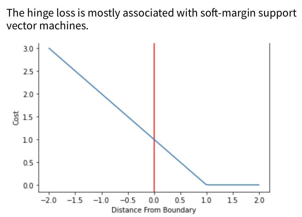
Hinge loss is a loss function primarily associated with maximum-margin classifiers, most notably Support Vector Machines (SVMs). It encourages not only correct classification but also a margin of separation between classes, thereby improving generalization performance. The theoretical foundations of hinge loss and margin-based learning are discussed in Statistical Learning Theory by Vapnik (1998).
-
A defining property of hinge loss is that it penalizes predictions that are either incorrect or insufficiently confident, even if they are technically correct. Correctly classified samples that lie close to the decision boundary still incur a positive loss if the margin constraint is not satisfied. This behavior explicitly enforces a minimum separation, or margin, between classes.
-
Hinge loss is a convex function with respect to the model parameters for linear classifiers. As a result, optimization problems involving hinge loss admit a unique global optimum and can be efficiently solved using convex optimization techniques. This property underpins the strong theoretical guarantees associated with SVMs, as described in Convex Optimization by Boyd and Vandenberghe (2004).
-
For a binary classification problem with target label \(t \in {-1, +1}\) and a classifier score \(y\), the hinge loss is defined as:
-
If the prediction is both correct and sufficiently far from the decision boundary such that \(t \cdot y \geq 1\), the loss is zero. Otherwise, the loss increases linearly as the margin violation grows.
-
In multi-class classification, hinge loss is extended to handle multiple classes by enforcing that the score assigned to the correct class exceeds the scores of all incorrect classes by at least a predefined margin. One common formulation is the multi-class SVM loss, which is described in Support Vector Machines for Pattern Classification by Cristianini and Shawe-Taylor (2000).
-
The hinge loss function is illustrated below:
-
Because hinge loss is not differentiable at the hinge point, subgradient methods are typically used during optimization. Variants such as the squared hinge loss introduce differentiability at the hinge point by squaring the margin violation, at the cost of increased sensitivity to outliers.
-
While hinge loss has largely been supplanted by cross-entropy loss in deep neural networks due to optimization convenience and probabilistic interpretability, it remains fundamental in margin-based learning and continues to be widely used in linear and kernel-based classifiers.
PolyLoss
-
PolyLoss was proposed in PolyLoss: A Polynomial Expansion Perspective of Classification Loss Functions by Leng et al. (2022). The work introduces a unifying framework for understanding and designing classification loss functions through the lens of polynomial expansion, offering a principled generalization of commonly used losses such as cross-entropy and focal loss.
-
In modern deep learning practice, cross-entropy loss and its variants, including focal loss, are the dominant choices for training classification models. While these losses perform well across a wide range of tasks, they represent only a narrow subset of possible loss function forms. PolyLoss is motivated by the observation that loss functions can be flexibly shaped to better suit specific datasets, noise characteristics, and optimization objectives.
-
The key insight of PolyLoss is that commonly used classification losses can be expressed as polynomial expansions of the model confidence term \(1 - p_t\), where \(p_t\) denotes the predicted probability assigned to the true class. This perspective is inspired by the Taylor series expansion of smooth functions and provides a systematic way to analyze and modify the behavior of loss functions across different confidence regimes.
-
Under this framework, focal loss can be interpreted as a horizontal shift in the polynomial coefficients relative to cross-entropy loss, effectively altering how the loss decays as the model’s confidence increases. Building on this insight, PolyLoss explores an alternative degree of freedom by vertically modifying the polynomial coefficients, enabling finer control over the contribution of higher-order terms.
-
Formally, PolyLoss augments the standard cross-entropy loss with a polynomial correction term:
\[\text { PolyLoss }=\sum_{i=1}^{n} \epsilon_{i} \frac{\left(1-p_{t}\right)^{i}}{i}+C E \text { Loss }\]-
where:
- \(p_t\) is the predicted probability of the true class,
- \(\epsilon_i\) are learnable or manually specified polynomial coefficients,
- \(n\) is the order of the polynomial expansion,
- and \(CE \text{ Loss}\) denotes the standard cross-entropy loss.
-
-
By adjusting the coefficients \(\epsilon_i\), PolyLoss allows practitioners to tailor the loss landscape, emphasizing or de-emphasizing specific confidence ranges during training. This flexibility can improve robustness to label noise, class imbalance, or optimization instability, depending on the task.
-
Empirical results reported by Leng et al. (2022) demonstrate that PolyLoss can consistently outperform both cross-entropy and focal loss across a variety of image classification benchmarks, while remaining simple to implement and computationally efficient.
-
In summary, PolyLoss provides a principled and extensible framework for understanding existing classification losses and for designing new ones. Rather than introducing ad hoc modifications, it grounds loss function design in a systematic polynomial expansion, offering both theoretical insight and practical performance benefits.
Generalized End-to-End Loss
-
Generalized End-to-End (GE2E) loss was introduced in Generalized End-to-End Loss for Speaker Verification by Wan et al. (2018) and presented at ICASSP. It was proposed to improve the efficiency and effectiveness of training speaker verification systems, particularly in comparison to earlier tuple-based end-to-end (TE2E) loss formulations.
-
Speaker verification is a metric learning problem in which the goal is to determine whether two speech segments belong to the same speaker. Rather than framing this as a conventional classification task, GE2E directly optimizes an embedding space in which utterances from the same speaker are close together, while utterances from different speakers are well separated. This formulation aligns closely with modern representation learning approaches used in biometrics and speech processing, as discussed in Speaker Verification: A Tutorial by Kinnunen and Li (2010).
-
A key limitation of the earlier TE2E loss was its reliance on explicit example selection and the construction of fixed tuples, which could lead to inefficient training and suboptimal gradient signals. GE2E addresses this limitation by operating on batches that contain multiple speakers and multiple utterances per speaker, enabling more informative comparisons within each training step.
-
Unlike TE2E, GE2E dynamically emphasizes difficult examples during training. Specifically, it increases the contribution of utterances that are easily confused with those of other speakers, thereby focusing learning on the most informative errors without requiring a separate hard example mining stage.
-
Formally, let \(\mathbf{e}_{ji}\) denote the embedding of the \(i^{th}\) utterance from the \(j\)-th speaker, and let \(\mathbf{S}_{ji,k}\) denote the similarity between \(\mathbf{e}_{ji}\) and the centroid of speaker \(k\). The GE2E loss for a single embedding is defined as:
-
This formulation closely resembles a softmax cross-entropy loss over speaker centroids, where the correct speaker centroid is treated as the target class. As a result, GE2E can be interpreted as applying a classification-style objective in an embedding space, while retaining the flexibility and generalization properties of metric learning. This connection is noted in Deep Metric Learning by Musgrave et al. (2020).
-
Empirically, Wan et al. (2018) demonstrate that GE2E converges faster and achieves better speaker verification performance than TE2E, while also simplifying the training pipeline. The loss function has since become a standard choice for training neural speaker embedding models and has influenced subsequent work in both speech and metric learning domains.
-
In summary, GE2E loss provides an efficient, stable, and effective objective for end-to-end training of speaker verification systems. By leveraging batch-level structure and dynamically emphasizing difficult examples, it bridges the gap between classification-based and metric-based learning approaches.
Additive Angular Margin Loss
-
Additive Angular Margin (AAM) Loss, commonly referred to as ArcFace, was proposed in ArcFace: Additive Angular Margin Loss for Deep Face Recognition by Deng et al. (2018). It was introduced to address the challenge of learning highly discriminative feature embeddings for large-scale face recognition tasks, where both intra-class compactness and inter-class separability are critical.
-
In deep face recognition, features are typically learned using deep convolutional neural networks (DCNNs). A central difficulty in this domain is designing loss functions that impose sufficiently strong geometric constraints on the learned embedding space. Earlier approaches addressed this challenge through different mechanisms:
- Centre loss enforces intra-class compactness by penalizing the Euclidean distance between deep features and their corresponding class centers.
- SphereFace introduces a multiplicative angular margin by modeling class weights as angular centers and penalizing angles between features and their corresponding class weights.
- Subsequent work explored additive margin formulations that improve training stability and interpretability.
-
ArcFace belongs to this latter family and introduces an additive angular margin directly in the angular space between normalized feature vectors and normalized class weight vectors. By operating in angular space, ArcFace achieves a clear geometric interpretation and directly optimizes the geodesic distance on a hypersphere. This formulation is discussed in detail in Deep Face Recognition: A Survey by Wang and Deng (2018).
-
Specifically, ArcFace enforces an angular margin by modifying the target logit from \(\cos(\theta)\) to \(\cos(\theta + m)\), where \(\theta\) is the angle between the feature vector and the corresponding class weight vector, and \(m\) is a fixed margin hyperparameter. This modification increases the decision boundary between classes in angular space, thereby improving discriminative power.
-
The ArcFace loss function is defined as:
\[-\frac{1}{N} \sum_{i=1}^{N} \log \frac{e^{s \left(\cos \left(\theta_{y_{i}}+m\right)\right)}}{e^{s \left(\cos \left(\theta_{y_{i}}+m\right)\right)}+\sum_{j=1, j \neq y_{i}}^{n} e^{s \left( \cos \theta_{j} \right)}}\]-
where:
- \(\theta_{j}\) is the angle between the feature vector \(x_i\) and the class weight vector \(W_j\),
- \(s\) is a scaling factor that controls the radius of the hypersphere and stabilizes optimization,
- \(m\) is the additive angular margin that enforces stricter class separation.
-
-
Both the feature vectors and the class weight vectors are L2-normalized prior to computing the cosine similarity, ensuring that the loss depends purely on angular relationships rather than vector magnitudes. This normalization is essential for the geometric interpretation of ArcFace and is one of the reasons for its empirical stability.
-
Deng et al. (2018) demonstrate that ArcFace consistently outperforms previous margin-based losses such as SphereFace and CosFace across multiple large-scale face recognition benchmarks, while remaining easy to implement and computationally efficient. The authors also release training data, code, and pretrained models, which has facilitated widespread adoption and reproducibility.
-
Although originally developed for face recognition, Additive Angular Margin Loss has since been successfully applied to other metric learning problems, including speaker verification and person re-identification, where discriminative embedding learning is equally important.
-
In summary, ArcFace provides a theoretically well-motivated and geometrically interpretable loss function that directly optimizes angular margins in normalized embedding spaces, leading to highly discriminative representations and strong empirical performance.
Dice Loss
-
Dice Loss is derived from the Sørensen–Dice coefficient, a similarity measure originally introduced in the 1940s to quantify the overlap between two finite sets. The coefficient was formalized in A Method of Establishing Groups of Equal Amplitude in Plant Sociology by Sørensen (1948). Its adoption in machine learning, particularly in medical image segmentation, reflects its suitability for tasks involving highly imbalanced foreground and background classes.
-
Dice Loss was popularized in the computer vision community by V-Net: Fully Convolutional Neural Networks for Volumetric Medical Image Segmentation by Milletari et al. (2016), where it was shown to outperform standard pixel-wise losses such as cross-entropy in scenarios with severe class imbalance. A more recent analysis and refinement of Dice Loss is presented in Rethinking Dice Loss for Medical Image Segmentation by Zhao et al. (2020).
-
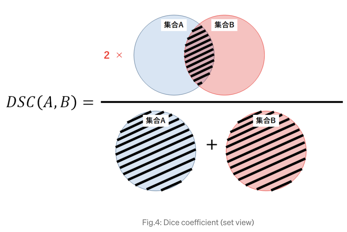
The Dice coefficient measures the similarity between a predicted segmentation and the ground truth segmentation by directly computing their overlap. Given predicted values \(p_i\) and ground truth labels \(g_i\) over \(N\) pixels or voxels, the Dice coefficient is defined as:
-
From a set-theoretic perspective, the Dice coefficient can be interpreted as twice the size of the intersection of two sets divided by the sum of their sizes. If the predicted and ground truth sets overlap perfectly, the Dice coefficient equals 1. If there is no overlap, the coefficient equals 0.
-
Because the Dice coefficient takes values in the interval \([0,1]\) and higher values indicate better agreement, Dice Loss is typically defined as:
-
Minimizing Dice Loss therefore directly maximizes the overlap between predicted and ground truth segmentations. This direct optimization of overlap distinguishes Dice Loss from pixel-wise losses, which treat each pixel independently and may be dominated by the majority class in imbalanced datasets.
-
Dice Loss is particularly effective in medical image segmentation tasks, such as tumor segmentation or organ delineation, where the foreground region may occupy only a small fraction of the image. In such settings, Dice Loss provides stronger gradient signals for the minority class than standard cross-entropy loss. A comparative analysis of segmentation losses is provided in A Survey on Loss Functions for Medical Image Segmentation by Taghanaki et al. (2020).
-
In practice, Dice Loss is often combined with cross-entropy loss to balance region-level overlap optimization with pixel-level classification accuracy. Variants such as soft Dice loss and generalized Dice loss further adapt the formulation to multi-class segmentation and extreme class imbalance scenarios.
-
In summary, Dice Loss offers a principled and effective objective for segmentation tasks characterized by class imbalance. By directly optimizing for spatial overlap, it aligns closely with evaluation metrics commonly used in medical imaging and other dense prediction problems.
Takeaways
-
For most classification problems, cross-entropy loss is the default and most widely adopted objective function. Its strong probabilistic foundation, favorable optimization properties, and compatibility with gradient-based learning make it suitable for both binary and multi-class classification tasks.
-
Variants of cross-entropy, such as focal cross-entropy, extend the standard formulation by reweighting samples based on prediction difficulty. In particular, focal loss assigns greater weight to hard-to-classify examples and is especially effective in scenarios with severe class imbalance, such as dense object detection.
-
Kullback–Leibler divergence is a closely related information-theoretic measure that quantifies the discrepancy between two probability distributions. In supervised classification with fixed targets, minimizing cross-entropy is equivalent to minimizing KL divergence up to an additive constant. However, KL divergence can be less stable in practice when estimated over small mini-batches due to fluctuations in empirical entropy.
-
Hinge loss is the original objective function used in support vector machines and margin-based classifiers. It emphasizes maximizing the margin between classes rather than modeling class probabilities. While hinge loss is convex and theoretically well-motivated for linear models, it is less commonly used in modern deep neural networks due to its non-probabilistic nature and less convenient optimization behavior.
-
More recent loss functions, such as PolyLoss, Additive Angular Margin Loss, and Generalized End-to-End Loss, demonstrate that classification loss design remains an active area of research. These losses incorporate geometric, polynomial, or batch-level structure to improve discriminative power and training efficiency in specialized domains such as face recognition, speaker verification, and imbalanced classification.
Regression Loss Functions
Mean Absolute Error (MAE) / L1 Loss
-
Mean Absolute Error (MAE), also known as L1 loss, is a standard loss function used for regression tasks. It measures the average magnitude of the errors between predicted values and ground-truth targets, without considering the direction of the errors. MAE directly computes the absolute deviation between predictions and observations and aggregates these deviations across the dataset.
-
Formally, MAE is defined as:
\[\mathrm{MAE}=\frac{1}{m} \sum_{i=1}^{m}\left|h(x^{(i)})-y^{(i)}\right|\]-
where:
- \(m\) is the number of samples,
- \(x^{(i)}\) denotes the \(i^{th}\) input sample,
- \(h(x^{(i)})\) is the model prediction for the \(i^{th}\) sample,
- \(y^{(i)}\) is the corresponding ground-truth target value.
-
-
From a statistical perspective, minimizing MAE corresponds to maximum likelihood estimation under a Laplace (double exponential) noise model. This contrasts with mean squared error, which assumes Gaussian noise. As a result, MAE is more robust to outliers, since errors grow linearly rather than quadratically with the magnitude of the deviation. This relationship is discussed in Pattern Recognition and Machine Learning by Bishop (2006).
-
MAE is particularly well suited for regression problems in which the target variable exhibits heavy-tailed noise or contains extreme values that should not dominate the learning process. Because it does not disproportionately penalize large errors, MAE provides a more balanced objective in the presence of outliers.
-
A practical implication of using MAE is that its gradient is constant almost everywhere, except at zero where it is not differentiable. In practice, this non-differentiability does not pose a major issue, as subgradient methods or automatic differentiation frameworks handle it seamlessly. However, the constant gradient magnitude can lead to slower convergence compared to squared-error losses in smooth regions of the loss surface.
-
It is important to distinguish between L1 loss as a regression objective and L1 regularization. While both involve absolute values, L1 loss measures prediction error, whereas L1 regularization penalizes the magnitude of model parameters to encourage sparsity. A discussion of L1 and L2 regularization can be found in The Elements of Statistical Learning by Hastie et al. (2009).
-
In summary, MAE is a robust regression loss that is less sensitive to outliers than squared-error losses. Its linear penalty structure makes it a natural choice when large deviations should not dominate training, albeit at the cost of potentially slower optimization dynamics.
Mean Squared Error (MSE) / L2 Loss
-
Mean Squared Error (MSE), also referred to as L2 loss, is one of the most commonly used loss functions for regression tasks. It measures the average of the squared differences between predicted values and ground-truth targets, thereby penalizing larger errors more strongly than smaller ones.
-
Formally, MSE is defined as:
\[\mathrm{MSE}=\frac{1}{m} \sum_{i=1}^{m}\left(y^{(i)}-\hat{y}^{(i)}\right)^{2}\]-
where:
- \(m\) is the number of samples,
- \(y^{(i)}\) is the ground-truth target for the \(i^{th}\) sample,
- \(\hat{y}^{(i)}\) is the corresponding model prediction.
-
-
From a probabilistic standpoint, minimizing MSE is equivalent to performing maximum likelihood estimation under the assumption that the observation noise follows a Gaussian distribution with constant variance. This assumption makes MSE particularly appropriate for regression problems in which the target variable is continuous and approximately normally distributed. This connection is discussed in Pattern Recognition and Machine Learning by Bishop (2006).
-
A key property of MSE is that its gradient grows linearly with the magnitude of the error. As a result, large deviations between predictions and targets receive disproportionately high penalties. This property can be beneficial when large errors are especially undesirable, but it also makes MSE sensitive to outliers, which can dominate the loss and distort the learning process.
-
MSE is differentiable everywhere and has a smooth quadratic loss surface. This smoothness often leads to faster and more stable convergence when optimized using gradient-based methods, particularly in comparison to MAE, whose gradient is discontinuous at zero.
-
It is important to distinguish between L2 loss and L2 regularization. While both involve squared terms, L2 loss penalizes prediction error, whereas L2 regularization penalizes large parameter values to reduce model complexity and improve generalization. A detailed discussion of this distinction can be found in The Elements of Statistical Learning by Hastie et al. (2009).
-
In summary, MSE is a smooth and analytically convenient loss function that performs well when the underlying noise is Gaussian and outliers are rare. However, in datasets with heavy-tailed noise or significant outliers, its sensitivity to large errors can lead to suboptimal performance compared to more robust alternatives.
Why Is Mean Squared Error Generally Unsuitable for Classification?
-
Mean Squared Error (MSE) is generally ill-suited for classification tasks because it relies on inappropriate statistical assumptions and leads to unfavorable optimization behavior when combined with standard classification models. These issues arise from a mismatch between the nature of classification targets and the loss function’s underlying assumptions, as well as from the resulting gradient dynamics during training.
-
A clear and accessible discussion of these limitations, illustrated primarily in the binary classification setting, is provided in Why Using Mean Squared Error (MSE) Cost Function for Binary Classification Is a Bad Idea?. Although the article focuses on binary classification, the arguments extend directly to multi-class classification.
Mismatch with the underlying data-generating distribution
-
Minimizing MSE corresponds to maximum likelihood estimation under a Gaussian observation model with additive noise. From a probabilistic perspective, this assumes that the target variable is continuous and normally distributed around the model’s prediction. This assumption is closely related to Gaussian conjugate priors and linear regression models, as discussed in the Wikipedia article on Conjugate prior.
-
Classification targets, however, are discrete rather than continuous. In binary classification, labels are naturally modeled using a Bernoulli distribution, while in multi-class classification they are modeled using categorical or multinomial distributions. Under these assumptions, the appropriate loss functions arise from the negative log-likelihood of these distributions, yielding binary cross-entropy and categorical cross-entropy, respectively.
-
This probabilistic mismatch means that MSE is optimizing the wrong likelihood model for classification tasks. In contrast, cross-entropy loss directly corresponds to maximum likelihood estimation under the correct discrete distributions. This distinction is standard in statistical learning theory and is described in The Elements of Statistical Learning by Hastie et al. (2009) and Pattern Recognition and Machine Learning by Bishop (2006).
Unfavorable optimization properties for classification models
-
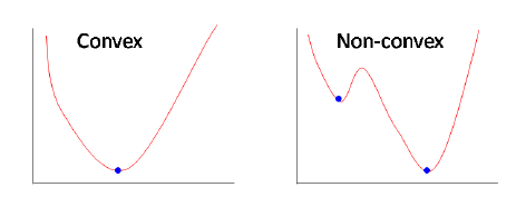
When MSE is combined with common classification output layers, such as the sigmoid function for binary classification or the softmax function for multi-class classification, the resulting objective function is generally non-convex with respect to the model parameters.
-
A non-convex objective admits multiple local minima and saddle points, which complicates optimization and weakens convergence guarantees. This behavior contrasts with logistic regression and softmax regression trained using cross-entropy loss, which yield convex optimization problems for linear models.
-
The conceptual difference between convex and non-convex objectives is illustrated in the following figure (source):
-
Convex objectives guarantee the existence of a unique global minimum, making optimization more reliable and interpretable. This property is discussed extensively in Convex Optimization by Boyd and Vandenberghe (2004).
-
Using MSE in classification forfeits this advantage, as it is fundamentally designed for real-valued targets defined over \((-\infty, \infty)\), whereas classification models output probabilities constrained to the interval \((0,1)\) and, in the multi-class case, to the probability simplex.
Practical implications for learning dynamics
-
MSE penalizes errors using squared Euclidean distance, which is poorly aligned with the geometry of probability distributions. As predicted probabilities approach 0 or 1, the gradients produced by MSE tend to vanish, especially when combined with sigmoid or softmax activations. This leads to slow learning and poor correction of confident but incorrect predictions.
-
In contrast, cross-entropy loss applies a logarithmic penalty that grows rapidly when the model assigns low probability to the correct class. This results in stronger and more informative gradients, particularly for misclassified examples, and leads to faster and more stable convergence in practice.
-
The differences in gradient behavior and optimization dynamics between MSE and cross-entropy loss are analyzed in detail in Pattern Recognition and Machine Learning by Bishop (2006) and in Deep Learning by Goodfellow et al. (2016).
-
In summary, MSE is inappropriate for classification because it assumes an incorrect noise model, leads to inferior optimization properties, and produces weak gradient signals in probabilistic classifiers. Cross-entropy loss, derived from the correct likelihood model, avoids these issues and is therefore the preferred objective for classification tasks.
Root Mean Squared Error (RMSE)
-
Root Mean Squared Error (RMSE) is a widely used metric for evaluating the accuracy of regression models that predict continuous-valued outcomes. It represents the square root of the mean of the squared differences between predicted values and observed values. These differences are referred to as residuals when computed on the training data and as prediction errors when computed on unseen data.
-
RMSE is commonly used in fields such as forecasting, climatology, econometrics, and regression analysis due to its interpretability and strong connection to mean squared error. Because RMSE is expressed in the same units as the target variable, it provides an intuitive measure of the typical magnitude of prediction error.
-
The RMSE of an estimator \(\hat{\theta}\) with respect to the true parameter \(\theta\) is defined as:
\[\text{RMSE}(\hat{\theta}) = \sqrt{\text{MSE}(\hat{\theta})}\]- where the mean squared error is given by:
-
In this formulation:
- \(\hat{\theta}_i\) denotes the predicted value for the \(i^{th}\) observation,
- \(\theta_i\) denotes the corresponding observed (true) value,
- \(n\) is the total number of observations.
-
From a statistical perspective, RMSE inherits the properties of MSE. In particular, minimizing RMSE is equivalent to minimizing MSE, since the square root is a monotonic transformation. As a result, RMSE and MSE yield identical optimal solutions during training, although RMSE is often preferred for reporting and evaluation due to its interpretability.
-
Like MSE, RMSE disproportionately penalizes large errors due to the squaring operation. This makes RMSE sensitive to outliers but also ensures that large deviations are strongly reflected in the error metric. This property can be desirable in applications where large prediction errors are especially costly.
-
In summary, RMSE is an interpretable and widely used regression error metric that provides a scale-consistent measure of prediction accuracy. While it shares the same sensitivity to outliers as MSE, its expression in the original units of the target variable makes it particularly useful for model evaluation and comparison.
Normalized Mean Absolute Error (NMAE)
-
Normalized Mean Absolute Error (NMAE) is a scale-invariant variant of the Mean Absolute Error (MAE) that expresses prediction error relative to a normalization factor derived from the target variable. By removing the dependence on absolute units, NMAE enables more meaningful comparisons of model performance across datasets with different scales or measurement units.
-
Like MAE, NMAE measures the average magnitude of prediction errors without considering their direction. The key distinction lies in the normalization step, which rescales the error to make it dimensionless and interpretable in relative terms.
-
NMAE is defined as:
-
where:
- \(\| \hat{\theta}_i - \theta_i \|\) is the absolute error for the \(i^{th}\) prediction,
- \(n\) is the number of observations,
- \(\text{norm}\) is a normalization constant.
-
The choice of normalization factor depends on the application context and the desired interpretation. Common normalization choices include:
- the range of the target variable, \(\max(\theta) - \min(\theta)\),
- the mean of the target variable, \(\mathrm{mean}(\theta)\),
- a known maximum possible value of the target variable.
-
Normalizing by the range yields a metric bounded between 0 and 1 when predictions lie within the observed range of the data, while normalization by the mean expresses error as a fraction of the typical target magnitude. Each choice has different interpretive implications, and care must be taken to ensure consistency when comparing NMAE values across studies.
-
From a statistical standpoint, NMAE retains the robustness properties of MAE, including reduced sensitivity to outliers relative to squared-error metrics. However, the normalization step introduces dependence on dataset-specific statistics, which may vary across samples or experimental conditions.
-
In summary, NMAE provides a relative, unit-free measure of regression error that is particularly useful for cross-dataset comparisons and benchmarking. Its interpretability and robustness make it a practical alternative to absolute error metrics when scale invariance is required.
Huber Loss (Smooth L1 Loss / Smooth Mean Absolute Error)
-
Huber loss is a regression loss function designed to combine the desirable properties of Mean Squared Error (MSE) and Mean Absolute Error (MAE). It is less sensitive to outliers than squared-error loss while remaining differentiable at zero, unlike absolute-error loss. Huber loss was originally introduced in robust statistics in Robust Estimation of a Location Parameter by Huber (1964).
-
The key idea behind Huber loss is to apply a quadratic penalty to small errors, encouraging smooth optimization behavior, and a linear penalty to large errors, reducing the influence of outliers. This makes Huber loss particularly effective in regression problems where the data are mostly well-behaved but may contain occasional extreme values.
-
Huber loss introduces a hyperparameter \(\delta\) that determines the threshold at which the loss transitions from quadratic to linear. To ensure smoothness at the transition point, additional terms are included so that both the loss value and its first derivative are continuous.
-
Formally, the Huber loss for a residual \(a\) is defined as:
\[L_{\delta}(a)= \begin{cases} \frac{1}{2} a^{2} & \text { for }|a| \leq \delta \\ \delta \cdot\left(|a|-\frac{1}{2} \delta\right) & \text { otherwise} \end{cases}\]-
where:
- \(a\) is the prediction error, typically defined as the difference between the predicted and true values,
- \(\delta\) is a positive threshold parameter controlling the transition between the quadratic and linear regimes.
-
-
For errors with magnitude smaller than \(\delta\), the loss behaves like MSE, promoting stable and efficient convergence near the optimum. For errors with magnitude larger than \(\delta\), the loss behaves like MAE, limiting the contribution of outliers to the overall objective.
-
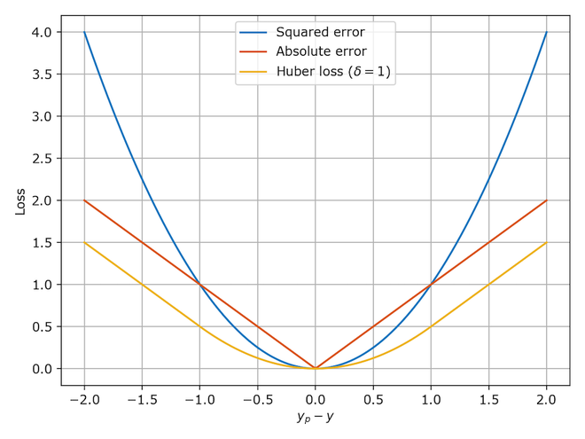
In practice, the residual \(a\) is often expressed explicitly as \(a = y - f(x)\), yielding the equivalent formulation:
- The following diagram (source) compares Huber loss with squared loss and absolute loss, highlighting its hybrid behavior:
-
Huber loss is widely used in practice, including in object detection frameworks such as Fast R-CNN, where it is referred to as Smooth L1 loss. Its robustness and differentiability make it well suited for deep learning applications that require stable gradient-based optimization.
-
In summary, Huber loss provides a principled compromise between sensitivity and robustness. By combining the smoothness of MSE with the outlier resistance of MAE, it offers reliable performance across a wide range of regression problems.
Asymmetric Huber loss
-
Asymmetric Huber loss is a variant of the standard Huber loss designed to treat overestimation and underestimation errors differently. While the classical Huber loss penalizes positive and negative errors symmetrically, the asymmetric formulation introduces differential weighting to reflect scenarios in which the costs of overprediction and underprediction are not equal.
-
This asymmetry is particularly useful in applications such as estimated time of arrival (ETA) prediction, demand forecasting, and risk-sensitive regression tasks, where underestimation and overestimation can have distinct practical or economic consequences.
-
As in standard Huber loss, the asymmetric version applies a quadratic penalty to small errors and a linear penalty to large errors. However, for errors beyond the threshold \(\delta\), different scaling factors are applied depending on the sign of the error.
-
The asymmetric Huber loss can be defined as:
\[L_{\delta}(a) = \begin{cases} \frac{1}{2}a^2 & \text{for } |a| \leq \delta, \\ \delta\left(|a| - \frac{1}{2}\delta\right) & \text{for } a > \delta, \\ \alpha\delta\left(|a| - \frac{1}{2}\delta\right) & \text{for } a < -\delta \end{cases}\]-
where:
- \(a\) is the prediction error, typically defined as the difference between the predicted value and the true value,
- \(\delta\) is the threshold at which the loss transitions from quadratic to linear behavior,
- \(\alpha\) is an asymmetry parameter that controls the relative penalty applied to underestimation errors (or, depending on the sign convention, overestimation errors).
-
-
When \(\alpha = 1\), the asymmetric Huber loss reduces to the standard symmetric Huber loss. Values of \(\alpha\) greater than 1 increase the penalty for one direction of error, while values less than 1 reduce it.
-
By explicitly encoding asymmetric error costs into the loss function, this formulation allows the learning objective to better reflect domain-specific priorities. This can lead to improved practical performance even if traditional symmetric error metrics appear similar.
-
In summary, asymmetric Huber loss extends the robustness and smoothness of standard Huber loss to settings with asymmetric error sensitivities. It provides a flexible and interpretable mechanism for incorporating domain knowledge about error costs directly into the training objective.
Takeaways
-
Regression loss functions are designed to measure discrepancies between continuous-valued predictions and ground-truth targets. The choice of loss function implicitly encodes assumptions about the noise distribution, the relative importance of small versus large errors, and the desired robustness to outliers.
-
MSE and its square-rooted variant, RMSE, are appropriate when the target noise is approximately Gaussian and large errors should be penalized strongly. Their smooth quadratic form often leads to stable and efficient optimization, but they are sensitive to outliers.
-
MAE and its normalized variant, NMAE, provide greater robustness to outliers by penalizing errors linearly. These losses are well suited for heavy-tailed noise distributions but may result in slower convergence due to their constant-gradient behavior.
-
Huber loss and its smooth variants offer a principled compromise between MSE and MAE. By behaving quadratically for small errors and linearly for large errors, they combine stable optimization with robustness to outliers and are widely used in practice, particularly in deep learning systems.
-
Asymmetric regression losses, such as asymmetric Huber loss, extend these ideas further by allowing different penalties for overestimation and underestimation. These losses are especially valuable in applications where error costs are direction-dependent and domain-specific considerations must be reflected in the training objective.
Ranking Loss
-
Ranking loss functions arise in learning-to-rank, metric learning, and similarity learning settings, where the objective is not to predict an absolute label or value, but rather to learn a relative ordering or preference among items. These losses are widely used in information retrieval, recommender systems, face recognition, and representation learning. A comprehensive overview of learning-to-rank methods is provided in Learning to Rank for Information Retrieval by Liu (2009).
-
Ranking loss is referred to by several closely related terms, reflecting differences in perspective rather than fundamentally different objectives:
- Ranking Loss originates from information retrieval and emphasizes learning an ordering over items.
- Margin Loss highlights the enforcement of a margin between positive and negative pairs in score or distance space.
- Contrastive Loss emphasizes comparing similar and dissimilar samples, typically in pairwise settings.
- Triplet Loss refers specifically to losses that operate on anchor–positive–negative triplets.
- Hinge Loss is the classical max-margin objective used in support vector machines and is closely related to several ranking formulations.
-
Although these terms are sometimes used interchangeably, they emphasize different structural aspects of the learning problem. In practice, many ranking and metric learning losses share common mathematical foundations.
-
Ranking loss functions are particularly flexible in terms of supervision requirements. Rather than requiring explicit class labels or numerical targets, they often rely only on relative similarity information. For example, in face verification datasets, it is sufficient to know whether two images belong to the same individual or to different individuals. This weak supervision makes ranking losses attractive in domains where absolute labels are difficult to obtain.
-
To apply a ranking loss, a model first maps each input instance to a vector representation, or embedding, using a feature extractor such as a convolutional or transformer-based neural network. A similarity or distance function, such as cosine similarity or Euclidean distance, is then applied to pairs or sets of embeddings. The loss function encourages embeddings of similar instances to be closer together than embeddings of dissimilar instances by at least a specified margin.
-
Importantly, ranking losses do not attempt to enforce absolute values for embeddings. Instead, they focus exclusively on relative distances or scores. This relative formulation has been shown to yield highly transferable and semantically meaningful representations, as discussed in Deep Metric Learning: A Survey by Musgrave et al. (2020).
-
In the following subsections, three widely used ranking loss families are discussed: margin-based ranking losses, probabilistic pairwise losses, and contrastive or triplet-based losses. Each formulation reflects a different trade-off between computational efficiency, optimization stability, and representational power.
Bayesian Personalized Ranking (BPR) Loss
-
Bayesian Personalized Ranking (BPR) loss was introduced in BPR: Bayesian Personalized Ranking from Implicit Feedback by Rendle et al. (2012). It was specifically designed for recommendation systems trained on implicit feedback data, such as clicks, views, or purchases, where explicit ratings are unavailable or unreliable.
-
In implicit feedback settings, the absence of an interaction does not necessarily indicate negative preference. Instead, BPR assumes a relative preference structure: for a given user, observed interactions are preferred over unobserved ones. The objective of BPR is therefore to learn personalized rankings rather than absolute relevance scores. A broader discussion of implicit-feedback recommendation is provided in Collaborative Filtering for Implicit Feedback Datasets by Hu et al. (2008).
-
BPR is a pairwise ranking loss that optimizes the probability that a user \(u\) prefers item \(i\) over item \(j\), where \(i\) is an observed (positive) interaction and \(j\) is an unobserved (assumed negative) interaction. The learning objective is derived from a Bayesian formulation but results in a simple and efficient optimization criterion.
Definition
-
The BPR loss is defined as:
\[\mathcal{L}_{\text{BPR}} = - \sum_{(u, i, j) \in D} \log(\sigma(\hat{y}_{uij})) + \lambda |\Theta|^2\]-
where:
- \(\sigma\) is the sigmoid function,
- \(\hat{y}_{uij} = \hat{y}_{ui} - \hat{y}_{uj}\) is the difference between the predicted scores for user \(u\) on the observed item \(i\) and the unobserved item \(j\),
- \(\Theta\) denotes the model parameters,
- \(\lambda\) is a regularization coefficient,
- \(D\) is the set of sampled user–item–item triples.
-
-
Maximizing \(\sigma(\hat{y}_{uij})\) encourages the model to assign a higher score to observed items than to unobserved ones. The logarithm ensures smooth gradients and numerical stability.
-
An alternative formulation extends BPR to multiple negative samples per positive interaction:
\[L_s = -\frac{1}{N_S} \sum_{j=1}^{N_S} \log(\sigma(\hat{r}_{s,i} - \hat{r}_{s,j}))\]-
where:
- \(N_S\) is the number of negative samples,
- \(\hat{r}_{s,k}\) denotes the predicted score for item \(k\) in a given session or context,
- \(i\) is the observed (positive) item,
- \(j\) indexes the sampled negative items.
-
Characteristics
- BPR explicitly optimizes ranking quality rather than pointwise prediction accuracy, making it well aligned with evaluation metrics such as AUC and mean reciprocal rank.
- The sigmoid-based formulation yields smooth gradients and stable optimization behavior.
- Regularization plays a critical role in preventing overfitting, particularly in high-dimensional embedding models.
- Performance is highly sensitive to the negative sampling strategy, which determines which unobserved items are treated as negatives during training.
Applications
- BPR is most commonly used in matrix factorization and neural recommendation models to learn user and item embeddings.
- It is particularly effective in large-scale recommender systems where implicit feedback is abundant and explicit ratings are sparse or unavailable.
Advantages
- Directly optimizes personalized ranking objectives.
- Well suited for implicit feedback datasets.
- Computationally efficient and easy to integrate with latent factor models.
Limitations
- The pairwise formulation increases computational complexity relative to pointwise losses.
- The assumption that all unobserved interactions are negative may not hold in all domains.
- Model performance depends heavily on the choice and diversity of negative samples.
Multiple Negative Ranking Loss
-
Multiple Negative Ranking (MNR) Loss was introduced in Efficient Natural Language Response Suggestion for Smart Reply by Henderson et al. (2017) at Google. It is a ranking-based contrastive loss designed for representation learning in scenarios where only positive pairs are available and explicit negative labels are absent.
-
MNR Loss is particularly well suited for retrieval and matching tasks involving paired data, such as paraphrase detection, duplicate question identification, query–document retrieval, and machine translation sentence alignment. In these settings, training data often consists solely of positive pairs, for example, pairs of semantically equivalent sentences or pairs of queries and relevant documents.
-
The core idea behind MNR Loss is to treat all non-matching pairs within a mini-batch as implicit negative examples. Given a batch of \(N\) positive pairs, each anchor is contrasted against its corresponding positive example and the remaining \(N-1\) examples in the batch, which serve as negatives. As a result, larger batch sizes naturally increase the number of negative samples and often lead to improved performance.
-
This loss formulation is closely related to noise-contrastive and InfoNCE-style objectives and can be interpreted as a softmax-based ranking loss that encourages correct pairs to have higher similarity scores than all other in-batch pairs. A broader discussion of in-batch negative sampling appears in Representation Learning with Contrastive Predictive Coding by van den Oord et al. (2018).
-
In natural language processing applications, MNR Loss has been shown to outperform pointwise softmax classification losses when training sentence embeddings for retrieval-oriented tasks. This behavior is discussed in Sentence-BERT: Sentence Embeddings using Siamese BERT-Networks by Reimers and Gurevych (2019).
-
As noted in (source), when using MNR Loss, neutral or contradictory pairs are typically excluded, and only positive entailment or matching pairs are retained. The negatives are generated implicitly through batching rather than explicit labeling.
-
Below is a code example from sbert.net, illustrating the use of Multiple Negatives Ranking Loss in practice:
from sentence_transformers import SentenceTransformer, losses, InputExample
from torch.utils.data import DataLoader

model = SentenceTransformer('distilbert-base-uncased')
train_examples = [InputExample(texts=['Anchor 1', 'Positive 1']),
    InputExample(texts=['Anchor 2', 'Positive 2'])]
train_dataloader = DataLoader(train_examples, shuffle=True, batch_size=32)
train_loss = losses.MultipleNegativesRankingLoss(model=model)
-
The effectiveness of MNR Loss is strongly influenced by batch composition and batch size. Larger batches provide more negative samples, improving discrimination but also increasing memory requirements. Practical trade-offs between batch size and computational efficiency are discussed in Next-Gen Sentence Embeddings with Multiple Negatives Ranking Loss.
-
In summary, Multiple Negative Ranking Loss provides a simple yet powerful mechanism for learning high-quality embeddings from positive-only data. By leveraging in-batch negatives and a softmax-based ranking objective, it enables efficient and scalable training of retrieval models across a wide range of domains.
Soft Pairwise Loss
-
Soft pairwise loss is a ranking-based objective function designed to learn relative preferences between instances by comparing their scores in a pairwise manner. Unlike hard margin–based losses, such as hinge loss, soft pairwise loss employs a smooth, differentiable formulation that yields stable gradients and facilitates optimization with gradient-based methods.
-
The primary objective of soft pairwise loss is to encourage instances that should be ranked higher to receive larger scores than instances that should be ranked lower, while penalizing violations of this ordering in a smooth and continuous fashion. This makes the loss well suited for ranking and metric learning tasks in which strict margin enforcement may be overly restrictive or unstable.
-
Soft pairwise loss is commonly used in applications such as information retrieval, recommendation systems, and representation learning, where relative ordering is more important than absolute prediction values. A general discussion of pairwise learning objectives appears in Learning to Rank for Information Retrieval by Liu (2009).
-
The soft pairwise loss can be defined as:
\[\mathcal{L}_{\text{soft-pairwise}} = \sum_{i=1}^{N} \sum_{j=1}^{N} \log\left(1 + \exp\left(-y_{i} \cdot (s_{i} - s_{j})\right)\right)\]-
where:
- \(s_i\) and \(s_j\) are the predicted scores for instances \(i\) and \(j\), respectively,
- \(y_i \in {+1, -1}\) indicates whether instance \(i\) should be ranked higher (\(+1\)) or lower (\(-1\)) relative to instance \(j\),
- \(N\) is the number of instances considered.
-
-
The logistic form of the loss ensures that larger score differences in the correct direction result in smaller loss values, while incorrect orderings incur a penalty that grows smoothly with the degree of violation. This behavior contrasts with hinge-based formulations, which impose a hard cutoff at the margin.
-
From a probabilistic perspective, soft pairwise loss can be interpreted as maximizing the likelihood that the ordering implied by the scores matches the observed pairwise preferences. This interpretation aligns it closely with logistic regression–based ranking objectives, as discussed in From RankNet to LambdaRank to LambdaMART: An Overview by Burges (2010).
-
In practice, the computational cost of evaluating all possible pairs scales quadratically with the number of instances in a batch. As a result, implementations often rely on sampling strategies or structured batching to reduce computational overhead while retaining informative comparisons.
-
In summary, soft pairwise loss provides a smooth and probabilistically motivated approach to learning relative orderings. Its differentiability and stable gradients make it a practical choice for ranking and similarity learning tasks where strict margin enforcement is unnecessary or undesirable.
Pairwise Logistic Loss
-
Pairwise logistic loss is a probabilistic ranking loss function commonly used in binary ranking and preference learning tasks. It operates on pairs of instances and encourages the model to assign higher scores to preferred or positive instances relative to non-preferred or negative instances.
-
Unlike pointwise classification losses, which evaluate predictions independently, pairwise logistic loss directly models relative ordering by comparing pairs of scores. This makes it particularly suitable for learning-to-rank problems in which the objective is to optimize relative preferences rather than absolute class labels. A detailed overview of pairwise ranking objectives is provided in Learning to Rank for Information Retrieval by Liu (2009).
-
The pairwise logistic loss can be defined as:
\[\mathcal{L}_{\text{pairwise-logistic}} = \sum_{i=1}^{N} \sum_{j=1}^{N} \log\left(1 + \exp\left(-(y_i - y_j) \cdot (s_i - s_j)\right)\right)\]-
where:
- \(s_i\) and \(s_j\) are the predicted scores for instances \(i\) and \(j\),
- \(y_i\) and \(y_j\) are the corresponding binary labels indicating class membership or preference,
- \(N\) is the number of instances under consideration.
-
-
This formulation encourages score differences \(s_i - s_j\) to be positive when \(y_i > y_j\) and negative otherwise. Violations of the desired ordering are penalized smoothly using a logistic function, which yields stable gradients even for large score differences.
-
From a probabilistic standpoint, pairwise logistic loss can be interpreted as modeling the probability that instance \(i\) should be ranked ahead of instance \(j\) using a logistic function. Minimizing the loss corresponds to maximizing the likelihood of observing the correct pairwise ordering, an idea originally introduced in RankNet, as described in Learning to Rank using Gradient Descent by Burges et al. (2005).
-
Compared to hinge-based ranking losses, pairwise logistic loss provides smoother optimization behavior and avoids non-differentiability at margin boundaries. However, like other pairwise losses, it incurs a computational cost that scales quadratically with the number of instances unless sampling or batching strategies are employed.
-
In summary, pairwise logistic loss offers a smooth, probabilistically grounded objective for learning relative orderings. Its strong theoretical foundation and favorable optimization properties make it a common choice in ranking, recommendation, and preference learning systems.
Pairwise Ranking Loss
-
The terminology surrounding pairwise loss and ranking loss is sometimes used inconsistently in the literature, as the two concepts are closely related and often overlap in practice. The distinction is best understood in terms of the structure of the supervision and the scope of the ordering being learned.
-
Pairwise loss functions operate on pairs or small tuples of samples, such as pairs or triplets. Their primary objective is to learn a representation or scoring function such that the relative relationship between two samples is preserved. Typical examples include contrastive loss and triplet loss, which focus on relative distances between samples rather than absolute labels.
-
Ranking loss functions, in a broader sense, aim to learn an ordering over a set of items. Rather than focusing exclusively on individual pairs, ranking losses are often concerned with minimizing the number of incorrectly ordered pairs within a list or set. This perspective is central to learning-to-rank problems in information retrieval and recommendation systems, as discussed in Learning to Rank for Information Retrieval by Liu (2009).
-
In practice, many ranking loss functions are implemented using pairwise comparisons, which explains why the terms pairwise loss and ranking loss are frequently used interchangeably. However, the conceptual emphasis differs: pairwise losses emphasize local comparisons, while ranking losses emphasize global ordering consistency.
-
Triplet loss, for example, is typically classified as a pairwise or metric learning loss because it compares distances between an anchor–positive pair and an anchor–negative pair. It does not explicitly optimize the ordering of a larger set of items, even though it can be used as a building block for ranking-based systems.
-
Conversely, ranking losses often aggregate pairwise violations across many item pairs to approximate a global ranking objective. This aggregation allows them to optimize ranking-specific evaluation metrics, such as mean reciprocal rank or normalized discounted cumulative gain, more directly.

-
As illustrated by the image above (source), pairwise ranking loss encourages the model to assign higher scores to instances that should be ranked ahead of others. The loss penalizes cases where the predicted ordering violates the ground-truth preference structure.
-
A common formulation of pairwise ranking loss uses a hinge-based objective:
\[\mathcal{L}_{\text{pairwise-ranking}} = \sum_{i=1}^{N} \sum_{j=1}^{N} \max(0, m - y_{i} \cdot (s_{i} - s_{j}))\]-
where:
- \(s_i\) and \(s_j\) are the predicted scores for instances \(i\) and \(j\),
- \(y_i \in {+1, -1}\) encodes the relative preference between the two instances,
- \(m\) is a margin hyperparameter that defines the minimum required separation between correctly ordered pairs.
-
-
This formulation penalizes violations of the desired ordering by enforcing that preferred instances receive scores at least \(m\) larger than non-preferred instances. Unlike probabilistic formulations, hinge-based ranking losses impose a hard margin, which can lead to sparse gradients once the margin constraint is satisfied.
-
Ranking losses are widely used in applications such as face recognition, image retrieval, document ranking, and recommendation systems. However, a key drawback is their computational complexity. Evaluating all pairwise comparisons within a batch has time complexity \(O(N^2)\), which can be prohibitive for large batch sizes. Practical implementations therefore rely on sampling strategies, structured batching, or approximate objectives. This limitation is discussed in (source).
-
In summary, pairwise ranking loss provides a flexible and intuitive mechanism for learning relative orderings by penalizing misordered pairs. While conceptually simple and widely applicable, its computational cost necessitates careful design choices in large-scale systems.
Triplet Loss
-
Triplet loss is a metric learning objective that operates on triplets of training examples rather than individual samples or pairs. It was introduced in FaceNet: A Unified Embedding for Face Recognition and Clustering by Schroff et al. (2015) and was originally developed for large-scale face recognition and clustering tasks.
-
Each training triplet consists of:
- an anchor sample \(A\),
- a positive sample \(P\) that belongs to the same class as the anchor,
- a negative sample \(N\) that belongs to a different class.
-
The objective of triplet loss is to learn an embedding space in which the distance between the anchor and the positive sample is smaller than the distance between the anchor and the negative sample by at least a fixed margin. This relative constraint directly enforces discriminative structure in the learned representation.

-
The triplet loss for a single triplet is defined as:
\[L = \max\left(d(A, P) - d(A, N) + \alpha, 0\right)\]-
where:
- \(d(\cdot, \cdot)\) is a distance function, commonly Euclidean distance or cosine distance,
- \(\alpha\) is a margin hyperparameter that controls the required separation between positive and negative pairs.
-
-
When the margin constraint is satisfied, the loss evaluates to zero and the corresponding triplet does not contribute to the gradient. Only triplets that violate the margin, often referred to as hard or semi-hard triplets, influence learning. Strategies for selecting informative triplets are therefore critical for effective training, as discussed in the original FaceNet paper and subsequent work such as In Defense of the Triplet Loss for Person Re-Identification by Hermans et al. (2017).
-
Triplet loss is particularly advantageous in scenarios where the set of classes is large or dynamic. For example, in face recognition systems, introducing a new identity would require retraining a standard classifier. In contrast, a model trained with triplet loss produces embeddings that can be compared directly using a distance metric, allowing new identities to be added without retraining the network.
-
From a geometric perspective, triplet loss shapes the embedding space by pulling samples of the same class closer together while pushing samples of different classes farther apart. Unlike classification losses, it does not explicitly model class probabilities and instead focuses on relative distances, making it well suited for retrieval, clustering, and verification tasks.
-
However, triplet loss can be computationally expensive, as the number of possible triplets grows cubically with the number of samples. Practical implementations therefore rely on efficient mining strategies and batch construction techniques to select informative triplets and reduce computational overhead.
-
In summary, triplet loss is a foundational objective in metric learning that directly optimizes relative distances in embedding space. Its flexibility and effectiveness have made it a standard choice for face recognition, person re-identification, and similarity-based retrieval tasks.
Margin Ranking Loss
-
Margin Ranking Loss (MRL) is a pairwise ranking objective designed to learn relative orderings between items by enforcing a margin between preferred and non-preferred instances. It is commonly used in ranking, metric learning, and knowledge representation tasks.
-
A representative formulation is presented in Adaptive Margin Ranking Loss for Knowledge Graph Embeddings via a Correntropy Objective Function by Nayyeri et al. (2019), where margin-based ranking objectives are used to distinguish positive and negative relational triples in knowledge graph embedding models.
-
Margin Ranking Loss operates on pairs of inputs \(X_1\) and \(X_2\) along with a label \(y \in {+1, -1}\) that indicates which input should be ranked higher. If \(y = 1\), the model is encouraged to assign a higher score to \(X_1\) than to \(X_2\); if \(y = -1\), the opposite ordering is enforced.
-
A common formulation of margin ranking loss is:
\[\mathcal{L}_{\text{margin}} = \sum_{i=1}^{N} \max(0, m - s_i^+ + s_i^-)\]-
where:
- \(s_i^+\) denotes the score of a positive (preferred) instance,
- \(s_i^-\) denotes the score of a negative (non-preferred) instance,
- \(m\) is a margin hyperparameter specifying the minimum required separation between the two scores.
-
-
In knowledge graph embedding settings, the loss is often written in terms of positive and negative triples:
\[\mathcal{L}=\sum_{(h, r, t) \in S^{+}} \sum_{\left(h^{\prime}, r^{\prime}, t^{\prime}\right) \in S^{-}}\left[f_{r}(h, t)+\gamma-f_{r}\left(h^{\prime}, t^{\prime}\right)\right]_{+}\]-
where:
- \(S^{+}\) and \(S^{-}\) denote sets of positive and negative triples,
- \(f_r(h, t)\) is a scoring function measuring the plausibility of a relational triple,
- \(\gamma\) is the margin parameter.
-
-
Margin Ranking Loss penalizes violations of the desired ordering by enforcing a hard margin constraint. Once the margin is satisfied, no further gradient signal is provided for that pair. This behavior encourages clear separation between positive and negative instances but can lead to sparse gradients in later stages of training.
-
Below is an example implementation in PyTorch, adapted from analyticsindiamag:
first_input = torch.randn(3, requires_grad=True)
Second_input = torch.randn(3, requires_grad=True)
target = torch.randn(3).sign()

ranking_loss = nn.MarginRankingLoss()
output = ranking_loss(first_input, Second_input, target)
output.backward()
print('input one: ', first_input)
print('input two: ', Second_input)
print('target: ', target)
print('output: ', output)
-
Margin ranking losses are conceptually extensions of hinge-based objectives and share similar properties with support vector machine losses. While they are intuitive and effective, they can be computationally expensive due to the quadratic number of pairwise comparisons within a batch. This limitation motivates the use of sampling strategies and approximate objectives in large-scale systems.
-
In summary, margin ranking loss provides a simple and interpretable mechanism for enforcing relative preferences through margin constraints. It is widely used in ranking, retrieval, and representation learning tasks, particularly when relative orderings are more important than calibrated probabilities.
Contrastive Loss
-
Contrastive loss is a distance-based objective function used in metric learning and contrastive representation learning. It was introduced in Dimensionality Reduction by Learning an Invariant Mapping by Hadsell et al. (2006) and is one of the earliest loss functions designed explicitly to learn embeddings rather than class probabilities.
-
The fundamental goal of contrastive loss is to learn a representation space in which similar samples are mapped close together, while dissimilar samples are mapped far apart. Unlike classification losses, contrastive loss does not require explicit class prediction and instead relies on pairwise similarity labels.
-
A brief clarification of terminology is useful:
- Contrastive learning refers broadly to learning representations by contrasting positive and negative examples.
- Multiple Negative Ranking Loss can be viewed as a contrastive loss that leverages in-batch negatives.
- Soft pairwise and pairwise logistic losses are typically categorized as ranking losses rather than contrastive losses, as they focus on ordering rather than explicit distance separation.
- Triplet loss is a contrastive loss, as it explicitly contrasts an anchor against positive and negative samples.
-
Contrastive loss operates on pairs of samples:
- a positive pair, consisting of two similar samples,
- a negative pair, consisting of two dissimilar samples.
-
Given:
- \(x_i\) as an anchor sample,
- \(x_i^{+}\) as a positive sample similar to \(x_i\),
- \(x_i^{-}\) as a negative sample dissimilar to \(x_i\),
- \(D(\cdot)\) as a distance function,
- \(m\) as a margin hyperparameter,
-
the contrastive loss for a single observation can be written as:
-
The first term encourages the model to minimize the distance between similar samples, while the second term enforces a minimum separation of \(m\) between dissimilar samples.
-
More formally, if \(\vec{X}\) denotes the input data and \(G_W(\vec{X})\) denotes the embedding produced by a neural network with parameters \(W\), the distance between two samples is defined as:
-
The contrastive loss over a dataset of \(P\) sample pairs is given by:
\[\begin{aligned} \mathcal{L}(W) &= \sum_{i=1}^P L\left(W,\left(Y, \vec{X}_1, \vec{X}_2\right)^i\right) \ L\left(W,\left(Y, \vec{X}_1, \vec{X}_2\right)^i\right) &= (1-Y) L_S\left(D_W^i\right)+Y L_D\left(D_W^i\right) \end{aligned}\]- where \(Y=0\) indicates a similar pair and \(Y=1\) indicates a dissimilar pair, and \(L_S\) and \(L_D\) denote the loss components for similar and dissimilar pairs, respectively.
-
A commonly used formulation is:
\[\begin{aligned} L\left(W, Y, \vec{X}_1, \vec{X}_2\right) = (1 - Y)\,\frac{1}{2}\left(D_W\right)^2 + Y\,\frac{1}{2}\left(\max\left(0, m - D_W\right)\right)^2 \end{aligned}\]- where \(m\) is a predefined margin that determines the minimum distance between dissimilar samples.
-
The gradient of the loss with respect to the network parameters is given by:
-
Contrastive loss is widely used in image retrieval, face verification, and signature verification tasks. During training, image pairs are labeled as similar or dissimilar, and the model learns embeddings that reflect these relationships.
-
The following formulation is commonly used in image retrieval:
\[y d^2+(1-y) \max (\operatorname{margin}-d, 0)^2\]-
where \(d\) is the Euclidean distance between two embeddings \(f_1\) and \(f_2\):
\[d=\left | f_1-f_2\right |_{2}\]
-
-
The margin parameter tightens the constraint by requiring dissimilar samples to be separated by at least the specified distance.
-
The effectiveness of contrastive loss in learning structured embedding spaces is illustrated in the results from the original paper:
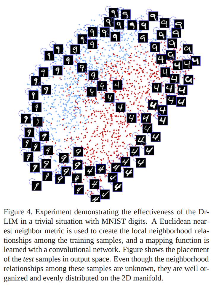
-
Contrastive loss has since inspired numerous extensions and variants. For example, cosine similarity–based contrastive objectives are used in CLIP by Radford et al. (2021), while normalized temperature-scaled contrastive losses such as InfoNCE are used in modern self-supervised learning frameworks.
-
In summary, contrastive loss is a foundational objective for learning distance-preserving representations. By explicitly pulling similar samples together and pushing dissimilar samples apart, it produces embeddings that are well suited for retrieval, clustering, and verification tasks.
InfoNCE Loss
-
InfoNCE loss is a contrastive loss function introduced in Contrastive Predictive Coding by van den Oord et al. (2018). It is a central objective in modern self-supervised and contrastive representation learning and is closely related to Noise-Contrastive Estimation (NCE).
-
The primary goal of InfoNCE is to learn representations that maximize mutual information between related variables, such as different views of the same data point or temporally adjacent observations. By contrasting a positive sample against a set of negative samples, the loss encourages the model to assign higher similarity to true pairs than to unrelated ones. A detailed discussion of mutual information–based objectives is provided in Mutual Information Neural Estimation by Belghazi et al. (2018).
-
InfoNCE can be interpreted as a multi-class classification problem in which the model must identify the correct positive sample among a set of candidates consisting of one positive and multiple negatives. The loss is implemented using a softmax followed by categorical cross-entropy.
-
Let \(c_t\) denote a context representation and \(x_{t+k}\) denote a future or related sample. Let \(f_k(x, c)\) be a scoring function measuring compatibility between \(x\) and \(c\). The InfoNCE loss is defined as:
\[\mathcal{L}_{\mathrm{N}}=-\underset{X}{\mathbb{E}}\left[\log \frac{f_{k}\left(x_{t+k}, c_{t}\right)}{\sum_{x_{j} \in X} f_{k}\left(x_{j}, c_{t}\right)}\right]\]-
where:
- \(X\) is a set containing one positive sample \(x_{t+k}\) and multiple negative samples,
- \(f_k(\cdot, \cdot)\) is typically implemented as an exponentiated similarity function, such as the exponential of a dot product or cosine similarity.
-
-
Minimizing this loss increases the score of the positive pair relative to all negative pairs in the denominator. As the number of negative samples increases, the InfoNCE objective becomes a tighter lower bound on the mutual information between \(x\) and \(c\), as shown in the original CPC paper.
-
InfoNCE has become the dominant loss function in modern contrastive learning frameworks. Notable examples include:
- A Simple Framework for Contrastive Learning of Visual Representations (SimCLR) by Chen et al. (2020),
- Momentum Contrast for Unsupervised Visual Representation Learning (MoCo) by He et al. (2020),
- Bootstrap Your Own Latent (BYOL) by Grill et al. (2020), which removes explicit negatives while retaining a related objective structure.
-
In practice, InfoNCE performance is strongly influenced by the number and diversity of negative samples, the temperature parameter used in the softmax normalization, and the choice of similarity function. These design choices affect both optimization stability and representation quality, as analyzed in Understanding Contrastive Representation Learning through Alignment and Uniformity by Wang and Isola (2020).
-
In summary, InfoNCE loss provides a principled and scalable contrastive objective that unifies ideas from information theory, probabilistic classification, and representation learning. Its effectiveness and flexibility have made it a foundational component of modern self-supervised learning methods.
SimCLR Loss (NT-Xent Loss)
-
The SimCLR loss, commonly referred to as the Normalized Temperature-scaled Cross-Entropy (NT-Xent) loss, was introduced in A Simple Framework for Contrastive Learning of Visual Representations by Chen et al. (2020). It is a specific instantiation of the InfoNCE objective tailored for large-scale contrastive self-supervised learning, particularly in computer vision.
-
SimCLR operates by generating two correlated views of each data sample through stochastic data augmentations, such as random cropping, color jittering, and Gaussian blur. Each original sample thus yields a positive pair, while all other augmented samples within the same mini-batch are treated as negatives. This design eliminates the need for explicit negative sampling beyond the mini-batch itself.
-
Let \({z_k}_{k=1}^{2N}\) denote the normalized embeddings of \(2N\) augmented samples obtained from \(N\) original data points, where each original sample contributes exactly two augmented views. For a positive pair \((i, j)\) corresponding to two views of the same sample, the NT-Xent loss for anchor \(i\) is defined as:
\[\ell_{i,j} = -\log \frac{\exp(\mathrm{sim}(z_i, z_j) / \tau)}{\sum_{k=1}^{2N} \mathbb{1}_{[k \neq i]} \exp(\mathrm{sim}(z_i, z_k) / \tau)}\]-
where:
- \(\mathrm{sim}(z_i, z_j)\) denotes a similarity function, typically cosine similarity,
- \(\tau\) is a temperature hyperparameter that controls the concentration of the distribution,
- \(\mathbb{1}_{[k \neq i]}\) excludes the anchor itself from the denominator.
-
-
The final SimCLR loss is computed by symmetrizing the objective across both directions of each positive pair and averaging over all \(N\) pairs in the batch. This formulation is equivalent to an InfoNCE loss with in-batch negatives and has a clear interpretation as a multi-class classification problem over augmented views.
-
A critical empirical finding of Chen et al. (2020) is that SimCLR performance scales strongly with batch size, as larger batches provide more negative samples, leading to better representation quality. This observation reinforces the close connection between contrastive learning performance and the number of effective negatives, as also discussed in Understanding Contrastive Representation Learning through Alignment and Uniformity by Wang and Isola (2020).
-
SimCLR further introduces a projection head, typically a small multilayer perceptron, applied on top of the encoder during training. The contrastive loss is computed in the projected space, while the representations before projection are used for downstream tasks. This design choice was shown to significantly improve downstream performance.
-
In summary, the SimCLR loss is a practical and influential specialization of the InfoNCE objective. By combining aggressive data augmentation, in-batch negatives, temperature scaling, and projection heads, it demonstrates that simple contrastive objectives can learn high-quality representations without labels, and it has inspired a wide range of subsequent self-supervised learning methods.
Losses in Deep Learning-based Reinforcement Learning
-
Deep learning has had a transformative impact on reinforcement learning (RL), enabling agents to operate in environments with high-dimensional state and action spaces. By combining neural networks with classical RL algorithms, deep reinforcement learning methods can approximate complex value functions and policies that were previously intractable. A comprehensive overview is provided in Human-level control through deep reinforcement learning by Mnih et al. (2015).
-
In deep reinforcement learning, loss functions play a central role in guiding the optimization of value functions, policies, or both. Unlike supervised learning, where targets are fixed, RL losses are defined in terms of bootstrapped estimates and stochastic returns, which introduces additional sources of variance and instability. This section outlines two fundamental loss formulations: Q-value loss and policy gradient loss.
Q-Value Loss
-
In value-based reinforcement learning methods, such as Deep Q-Networks (DQN), the objective is to learn an action-value function \(Q(s, a)\) that estimates the expected cumulative discounted reward obtained by taking action \(a\) in state \(s\) and following a given policy thereafter.
-
The optimal action-value function satisfies the Bellman optimality equation:
\[Q(s, a) = r + \gamma \max_{a'} Q(s', a')\]-
where:
- \(r\) is the immediate reward received after taking action \(a\) in state \(s\),
- \(\gamma \in [0,1]\) is the discount factor that controls the relative importance of future rewards,
- \(s'\) is the subsequent state.
-
-
In deep Q-learning, the Q-function is parameterized by a neural network, and training proceeds by minimizing the mean squared temporal-difference (TD) error between the predicted Q-value and a target value derived from the Bellman equation. The Q-value loss is therefore defined as:
- Minimizing this loss encourages consistency between the learned Q-function and the Bellman target. In practice, target networks and experience replay are employed to stabilize training, as described in the original DQN work by Mnih et al. (2015).
Policy Gradient Loss
-
Policy gradient methods take a fundamentally different approach by directly optimizing a parameterized policy \(\pi_\theta(a \mid s)\), which defines a probability distribution over actions given a state. Rather than estimating value functions explicitly, these methods seek to maximize the expected cumulative reward through gradient ascent.
-
The policy gradient theorem provides an expression for the gradient of the expected return with respect to the policy parameters. In practice, learning is framed as minimizing a loss function that is the negative expected return, yielding the policy gradient loss:
\[\mathcal{L}_{\text{PG}} = -\mathbb{E}\left[ \sum_{t=0}^{T} \log \pi_\theta(a_t \mid s_t) \cdot A(s_t, a_t) \right]\]-
where:
- \(A(s_t, a_t)\) is an advantage function that measures how much better action \(a_t\) is compared to the average action in state \(s_t\),
- \(T\) denotes the time horizon of an episode.
-
-
The use of advantage functions, as in Asynchronous Methods for Deep Reinforcement Learning by Mnih et al. (2016) and Proximal Policy Optimization Algorithms by Schulman et al. (2017), reduces variance and improves training stability.
-
Policy gradient losses are often augmented with additional terms, such as entropy regularization, to encourage exploration, or value-function losses in actor–critic architectures. These extensions do not alter the fundamental role of the policy gradient loss but improve empirical performance.
-
In summary, loss functions in deep reinforcement learning encode learning objectives that differ fundamentally from those in supervised learning. Q-value losses enforce Bellman consistency through squared TD errors, while policy gradient losses optimize stochastic policies by weighting log-probabilities with estimated advantages. Together, these objectives form the foundation of modern deep reinforcement learning algorithms.
Further Reading
- PyTorch Losses Documentation
- SBERT: Losses
- Understanding Ranking Loss, Contrastive Loss, Margin Loss, Triplet Loss, Hinge Loss and all those confusing names
- Understanding Categorical Cross-Entropy Loss, Binary Cross-Entropy Loss, Softmax Loss, Logistic Loss, Focal Loss and all those confusing names
- Next-Gen Sentence Embeddings with Multiple Negatives Ranking Loss
- A Gentle Introduction to Cross-Entropy for Machine Learning
- Things that confused me about cross-entropy
References
- Machine Learning Mastery
- ML CheatSheet
- Neptune.ai
- Section.ai
- After Academy
- Programmathically
- PapersWithCode: Focal Loss
- ArcFace Additive Angular Margin Loss for Deep Face Recognition
- Medium AnalyticsVidhya
- PolyLoss
- Generalized End-to-End Loss
- Wikipedia article on Huber loss
- Wikipedia article on Triplet loss
- Towards Data Science
- Papers With Code infoNCE
- Lilian Weng: Contrastive learning
- Dice Loss by Shuchen Du
- Margin Ranking Loss
- Margin Ranking Loss Official Paper
- Wikipedia: Kullback–Leibler divergence
- Kullback-Leibler Divergence Explained
- What is the difference Cross-entropy and KL divergence?
Citation
If you found our work useful, please cite it as:
@article{Chadha2020DistilledLossFunctions,
  title   = {Loss Functions},
  author  = {Chadha, Aman and Jain, Vinija},
  journal = {Distilled AI},
  year    = {2020},
  note    = {\url{https://vinija.ai}}
}