Primers • Hyperparameter Tuning
Hyperparameter Tuning
-
A plethora of hyperparameters are typically involved in the design of a deep neural network, including learning rate, batch size, number of layers, hidden units, regularization strength, optimizer choice, and architectural decisions. These parameters are not learned directly from data but must be specified prior to training, making their selection a critical part of model development Practical Recommendations for Gradient-Based Training of Deep Architectures by Bengio et al. (2012).
-
Formally, let \(\mathcal{D}*{train}\) and \(\mathcal{D}*{val}\) denote the training and validation datasets. Let \(\theta\) represent model parameters and \(\lambda \in \Lambda\) represent hyperparameters. Training involves solving:
- The goal of hyperparameter tuning is to find the optimal hyperparameters that minimize validation error:
-
This defines a nested optimization problem, often referred to as bilevel optimization Bilevel Programming for Hyperparameter Optimization and Meta-Learning by Franceschi et al. (2018). The outer loop optimizes hyperparameters, while the inner loop trains the model.
-
In practice, this optimization is extremely expensive because each evaluation of \(\lambda\) requires a full or partial training run. If training takes hours or days, even evaluating a few dozen hyperparameter configurations can be computationally prohibitive.
-
In most cases, the space of possible hyperparameters is far too large for exhaustive search. For example:
- A learning rate might vary over \([10^{-6}, 1]\) (continuous range)
- Network depth might range from 2 to 200 layers (discrete)
- Optimizer choice is categorical (SGD, Adam, RMSProp, etc.)
This leads to a high-dimensional, mixed-type search space \(\Lambda\) that is often non-convex, noisy, and expensive to evaluate Algorithms for Hyper-Parameter Optimization by Bergstra et al. (2011).
-
Additionally, the validation loss landscape \(\mathcal{L}_{val}(\theta^*(\lambda))\) is typically:
- Non-smooth due to stochastic training
- Non-convex with many local minima
- Expensive to evaluate
- Potentially noisy due to randomness in initialization and data sampling
-
These properties make classical optimization methods such as gradient descent difficult to apply directly in hyperparameter space. While gradient-based hyperparameter optimization exists, it often requires differentiability assumptions and significant engineering effort Gradient-Based Hyperparameter Optimization through Reversible Learning by Maclaurin et al. (2015).
-
As a result, hyperparameter tuning is often treated as a black-box optimization problem:
\[\min_{\lambda \in \Lambda} f(\lambda)\]- where \(f(\lambda) = \mathcal{L}_{val}(\theta^*(\lambda))\) is only observable through expensive evaluations.
-
Because of these challenges, a variety of search strategies have been developed, including:
- Grid search
- Random search
- Bayesian optimization
- Evolutionary algorithms
-
Hyperband and multi-fidelity methods
- Each method makes different assumptions about the structure of \(f(\lambda)\) and the cost of evaluation Hyperband: A Novel Bandit-Based Approach to Hyperparameter Optimization by Li et al. (2017).
-
In modern deep learning practice, efficient hyperparameter tuning is often as important as model architecture design itself. Empirical studies have shown that proper tuning can yield larger performance gains than switching model families Random Search for Hyper-Parameter Optimization by Bergstra & Bengio (2012).
Random Search and Grid Search
- Consider the following function \(f(x,y) = g(x) + h(y)\) over parameters \(x,y\) and the maximization problem:
-
Assume we only have access to \(f(x,y)\) through an oracle, meaning we can evaluate \(f\) at a certain point \((x,y)\), but we do not know the functional form of \(f\). This is the standard black-box optimization setting used in hyperparameter tuning Random Search for Hyper-Parameter Optimization by Bergstra & Bengio (2012).
-
A natural approach is grid search: choose candidate sets \(X = {x_1,\dots,x_m}\) and \(Y = {y_1,\dots,y_n}\), then evaluate every pair:
-
Grid search therefore requires:
\[|\mathcal{G}| = m \cdot n\]-
evaluations in two dimensions, and more generally:
\[|\mathcal{G}| = \prod_{i=1}^{d} m_i\]- evaluations for \(d\) hyperparameters. This exponential growth is one reason grid search becomes impractical in high-dimensional hyperparameter spaces Random Search for Hyper-Parameter Optimization by Bergstra & Bengio (2012).
-
-
We could also evaluate a numerical gradient in hyperparameter space:
-
However, unlike one step of model training, each evaluation of hyperparameters may require training a model to completion or near completion. This makes gradient-style finite difference search expensive and often infeasible Practical Recommendations for Gradient-Based Training of Deep Architectures by Bengio et al. (2012).
-
Now assume we know that:
-
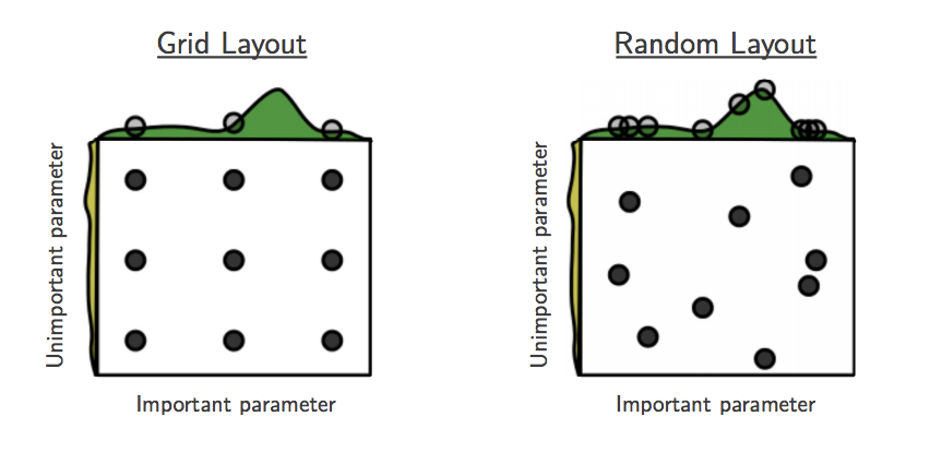
In this case, would grid search still be a good strategy? Since \(f\) mostly depends on \(x\), grid search wastes many evaluations testing different values of \(y\). In high-dimensional hyperparameter spaces, it is common for only a small subset of hyperparameters to matter strongly for performance Random Search for Hyper-Parameter Optimization by Bergstra & Bengio (2012).
-
Random search instead samples configurations independently from distributions over hyperparameters:
\[\lambda^{(i)} \sim p(\lambda), \quad i = 1,\dots,N\]- where \(\lambda\) denotes a hyperparameter configuration and \(N\) is the search budget.
-
For two hyperparameters, this might be written as:
-
The key advantage is that every random trial tests a new value of every hyperparameter. If only \(x\) matters, random search explores many more distinct values of \(x\) than grid search under the same evaluation budget Random Search for Hyper-Parameter Optimization by Bergstra & Bengio (2012).
-
An illustration of how random search can improve on grid search of hyperparameters. “This failure of grid search is the rule rather than the exception in high dimensional hyperparameter optimization” Random Search for Hyper-Parameter Optimization by Bergstra & Bengio (2012):
-
Random search is also flexible because each hyperparameter can be sampled from a distribution that matches its scale. For example, learning rates are often sampled log-uniformly rather than uniformly:
\[\log \eta \sim \mathcal{U}(\log \eta_{\min}, \log \eta_{\max})\]-
or equivalently:
\[\eta \sim \mathrm{LogUniform}(\eta_{\min}, \eta_{\max})\]
-
-
This is useful because learning rates often matter multiplicatively rather than additively Practical Recommendations for Gradient-Based Training of Deep Architectures by Bengio et al. (2012).
-
Grid search is still useful when the hyperparameter space is very small, when the practitioner has strong prior knowledge about useful values, or when reproducibility and systematic coverage are more important than efficiency. However, random search is usually a stronger baseline for large hyperparameter spaces Random Search for Hyper-Parameter Optimization by Bergstra & Bengio (2012).
-
What are weaknesses and assumptions of random search? Random search usually assumes that hyperparameters can be sampled independently:
- This can be limiting because hyperparameters are often correlated. For example, a larger batch size may require a different learning rate, and stronger regularization may interact with model size. Ideally, we would sample from a joint distribution:
that captures these dependencies.
- Another weakness is that random search does not use results from previous trials. After evaluating \(f(\lambda^{(1)}),\dots,f(\lambda^{(t)})\), the next configuration \(\lambda^{(t+1)}\) is still sampled without using the observed history:
- This motivates sequential model-based methods such as Bayesian optimization, which use previous evaluations to choose future configurations more intelligently Algorithms for Hyper-Parameter Optimization by Bergstra et al. (2011).
Bayesian Optimization
- Bayesian inference is a form of statistical inference that uses Bayes’ Theorem to incorporate prior knowledge when performing estimation. Bayes’ Theorem relates conditional and joint distributions of random variables. Let \(X\) denote the random variable representing model performance (e.g., validation accuracy or loss), and let \(\theta\) denote the hyperparameters. Then Bayes’ Rule gives:
-
In the context of hyperparameter optimization, we treat the objective function:
\[f(\theta) = \mathcal{L}_{val}(\theta)\]- as an unknown function that we want to minimize. Since evaluating \(f(\theta)\) is expensive, Bayesian optimization builds a probabilistic surrogate model of this function and uses it to guide the search Practical Bayesian Optimization of Machine Learning Algorithms by Snoek et al. (2012).
-
The key idea is to maintain a posterior distribution over possible objective functions given observed data:
-
where:
\[\mathcal{D}*t = {(\theta^{(i)}, f(\theta^{(i)}))}*{i=1}^{t}\]- is the set of previously evaluated hyperparameter configurations.
-
So the next question is: how could we use Bayes’ Rule to improve random search?
-
By placing a prior over functions and updating it with observed data, we can sample future hyperparameters in a way that is informed by past evaluations. Instead of sampling:
-
as in random search, Bayesian optimization selects:
\[\theta^{(t+1)} = \arg\max_{\theta} \alpha(\theta \mid \mathcal{D}_t)\]- where \(\alpha(\theta)\) is an acquisition function that quantifies the utility of evaluating \(\theta\) next.
-
Let’s reconsider the optimization problem of finding the maximum of \(f(x,y)\). A Bayesian optimization strategy would:
- Initialize a prior over functions \(p(f)\) (often a Gaussian process).
- Sample a point \((x,y)\) and evaluate \(f(x,y)\).
- Update the posterior \(p(f \mid \mathcal{D})\) using the observed data.
- Select the next point using an acquisition function.
- Repeat steps 2–4.
-
The goal is to approximate the unknown function \(f\). With each new data point, the posterior becomes more accurate, allowing the optimizer to make better decisions about where to evaluate next.
-
A common choice for the surrogate model is a Gaussian process (GP), which defines a distribution over functions:
\[f(\theta) \sim \mathcal{GP}(m(\theta), k(\theta, \theta'))\]- where \(m(\theta)\) is the mean function and \(k(\theta, \theta')\) is the kernel (covariance function). The GP provides both a mean prediction and uncertainty estimate for any \(\theta\) Gaussian Processes for Machine Learning by Rasmussen & Williams (2006).
-
Given observed data, the GP posterior predicts:
-
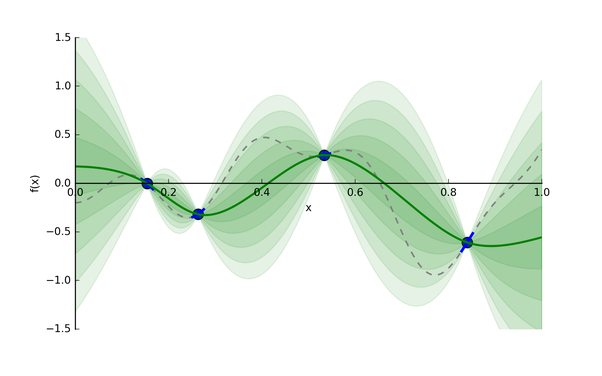
Let’s consider an example: say we want to find the minimum of some function whose expression is unknown. The function has one input and one output, and we’ve taken four different samples (the blue points).
-
A Gaussian process distribution, given four sampled data points in blue:
-
The Gaussian process provides a distribution of continuous functions that fit these points, which is represented in green. The darker the shade, the more likely the true function is within that region. The green line is the mean prediction, and the shaded regions correspond to uncertainty (standard deviation bands).
-
Now, given this useful model, what point should we evaluate next? We have two competing objectives:
- Exploitation: Choose a point with low predicted value based on the mean:
- Exploration: Choose a point with high uncertainty:
-
Balancing these two is the exploration-exploitation trade-off. This balance is achieved through an acquisition function.
-
A commonly used acquisition function is Expected Improvement (EI):
\[\alpha_{EI}(\theta) = \mathbb{E}[\max(f_{best} - f(\theta), 0)]\]- which can be computed in closed form under a Gaussian process model as:
-
where:
\[z = \frac{f_{best} - \mu(\theta)}{\sigma(\theta)}\]- and \(\Phi\) and \(\phi\) are the CDF and PDF of the standard normal distribution Practical Bayesian Optimization of Machine Learning Algorithms by Snoek et al. (2012).
-
Other acquisition functions include:
- Probability of Improvement (PI)
-
Upper Confidence Bound (UCB):
\[\alpha_{UCB}(\theta) = \mu(\theta) - \kappa \sigma(\theta)\]- where \(\kappa\) controls the exploration-exploitation trade-off.
-
With each iteration, “the algorithm balances its needs of exploration and exploitation” Bayesian Optimization Explained by Nogueira (2014):
-
Bayesian optimization is particularly effective when:
- Evaluations are expensive
- The number of hyperparameters is moderate (typically < 20)
- We want to minimize the number of training runs
-
If you’re interested in learning more or trying out the optimizer, here is a good Python code base for using Bayesian Optimization with Gaussian processes.
References
-
Random Search for Hyper-Parameter Optimization by Bergstra & Bengio (2012)
-
Algorithms for Hyper-Parameter Optimization by Bergstra et al. (2011)
-
Practical Bayesian Optimization of Machine Learning Algorithms by Snoek et al. (2012)
-
Gaussian Processes for Machine Learning by Rasmussen & Williams (2006)
-
Practical Recommendations for Gradient-Based Training of Deep Architectures by Bengio et al. (2012)
-
Bilevel Programming for Hyperparameter Optimization and Meta-Learning by Franceschi et al. (2018)
-
Gradient-Based Hyperparameter Optimization through Reversible Learning by Maclaurin et al. (2015)
-
Hyperband: A Novel Bandit-Based Approach to Hyperparameter Optimization by Li et al. (2017)
Citation
If you found our work useful, please cite it as:
@article{Chadha2020DistilledHyperparameterTuning,
  title   = {Hyperparameter Tuning},
  author  = {Chadha, Aman},
  journal = {Distilled AI},
  year    = {2020},
  note    = {\url{https://aman.ai}}
}