Primers • Hyperparameter Tuning
Hyperparameter Tuning
- A plethora of hyperparameters are typically involved in the design of a deep neural network. Finding the best set of hyperparameters is an optimization task in itself!
- In most cases, the space of possible hyperparameters is far too large for us to try all of them. Here are some strategies for solving this problem.
Random Search and Grid Search
- Consider the following function \(f(x,y) = g(x) + h(y)\) over parameters \(x,y\) and the maximization problem:
- Assume we only have access to \(f(x,y)\) through an oracle (i.e. we can evaluate \(f\) at a certain point \((x,y)\), but we do not know the functional form of \(f\)).
- The question is… how could we find the optimal values of \(x\) and \(y\)? A natural idea would be to choose a range for the values of \(x\) and \(y\) and sample a grid of points in this range.
- We could also evaluate a numerical gradient in the hyperparameter space. The challenge with this method is that unlike an iteration of model training, each evaluation of hyperparameters is very costly and long, making it infeasible to try many combinations of hyperparameters.
- Now assume we know that:
- In this case, would grid search still be a good strategy? The function $f$ mostly depends on \(x\). Thus, a grid search strategy will waste a lot of iterations testing different values of \(y\).
- If we have a finite number of evaluations of \((x,y)\), a better strategy would be randomly sampling \(x\) and \(y\) in a certain range, that way each sample tests a different value of each hyperparameter.
- An illustration of how random search can improve on grid search of hyperparameters. ‘This failure of grid search is the rule rather than the exception in high dimensional hyperparameter optimization.’ (Bergstra & Bengio, 2011):
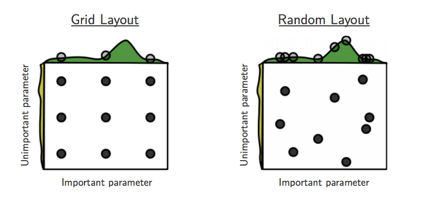
- What are weaknesses and assumptions of random search? Random search assumes that the hyperparameters are uncorrelated. Ideally, we would sample hyperparameters from a joint distribution that takes into account this understanding.
- Additionally, it doesn’t use the results of previous iterations to inform how we choose parameter values for future iterations. This is the motivation behind Bayesian optimization.
Bayesian Optimization
- Bayesian inference is a form of statistical inference that uses Bayes’ Theorem to incorporate prior knowledge when performing estimation. Bayes’ Theorem is a simple, yet extremely powerful, formula relating conditional and joint distributions of random variables. Let \(X\) be the random variable representing the quality of our model and \(\theta\) the random variable representing our hyperparameters. Then Bayes’ Rule relates the distributions \(P(\theta \mid X)\) (posterior), \(P(X\mid\theta)\) (likelihood), \(P(\theta)\) (prior) and \(P(X)\) (marginal) as:
- So the next question is: how could we use Bayes’ Rule to improve random search?
- By using a prior on our hyperparameters, we can incorporate prior knowledge into our optimizer. By sampling from the posterior distribution instead of a uniform distribution, we can incorporate the results of our previous samples to improve our search process.
-
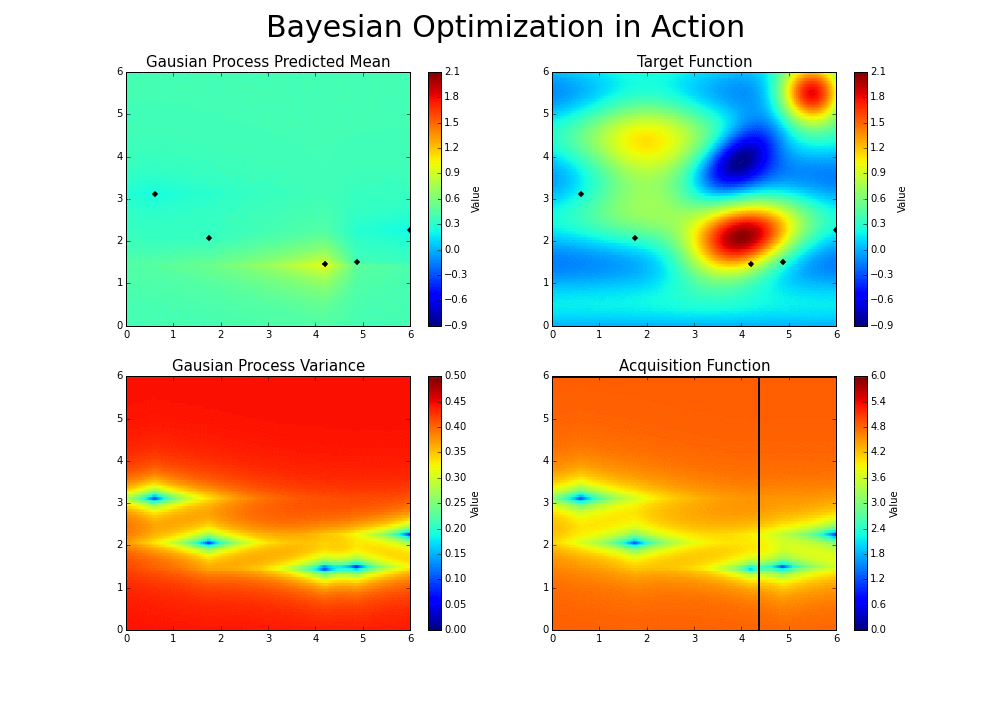
Let’s reconsider the optimization problem of finding the maximum of \(f(x,y)\). A Bayesian optimization strategy would:
- Initialize a prior on the parameters \(x\) and \(y\).
- Sample an point \((x,y)\) to evaluate \(f\) with.
- Use the result of \(f(x,y)\) to update the posterior on \(x,y\).
- Repeat 2 and 3.
- The goal is to guess the function, even if we cannot know its true form. By adding a new data point at each iteration, the algorithm can guess the function more accurately, and more intelligently choose the next point to evaluate to improve its guess. A Gaussian process is used to infer the function from samples of its inputs and outputs. It also provides a distribution over the possible functions given the observed data.
-
Let’s consider an example: say we want to find the minimum of some function whose expression is unknown. The function has one input and one output, and we’ve taken four different samples (the blue points).
- A Gaussian process distribution, given four sampled data points in blue:
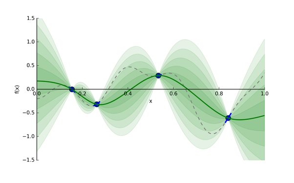
- The Gaussian process provides a distribution of continuous functions that fit these points, which is represented in green. The darker the shade, the more likely the true function is within that region. The green line is the mean guess of the “true” function, and each band of green is a half standard deviation of the Gaussian process distribution.
- Now, given this useful guess, what point should we evaluate next? We have two possible options:
- Exploitation: Evaluate a point that, based on our current model of likely functions, will yield a low output value. For instance, 1.0 could be an option in the above graph.
- Exploration: Get a datapoint on an area we’re most unsure about. In the graph above, we could focus on the zone between 0.65 and 0.75, rather than between 0.15 and 0.25, since we have a pretty good idea as to what’s going on in the latter zone. That way, we will will be able to reduce the variance of future guesses.
- Balancing these two is the exploration-exploitation trade-off. We choose between the two strategies using an acquisition function.
- With each iteration ‘the algorithm balances its needs of exploration and exploitation’ (Nogueira):
- If you’re interested in learning more or trying out the optimizer, here is a good Python code base for using Bayesian Optimization with Gaussian processes.
References
Citation
If you found our work useful, please cite it as:
@article{Chadha2020DistilledHyperparameterTuning,
  title   = {Hyperparameter Tuning},
  author  = {Chadha, Aman},
  journal = {Distilled AI},
  year    = {2020},
  note    = {\url{https://aman.ai}}
}