Primers • Generative Adversarial Networks (GANs)
- Introduction
- Underlying principle
- Background: What is a Generative Model?
- Modeling Probabilities
- Generative Models Are Hard
- Overview of GAN Structure
- The Generator
- The Discriminator
- GAN Training
- Loss Functions
- Common Problems
- GAN Variations
- Text-to-Speech
- References
- Citation
Introduction
- Introduced by Goodfellow et al. in NeurIPS (2014), generative adversarial networks (GANs) are an exciting recent innovation in machine learning. GANs are generative models: they create new data instances that resemble your training data. For example, GANs can create images that look like photographs of human faces, even though the faces don’t belong to any real person.
- The following images of four photorealistic faces were created by a GAN created by NVIDIA:

Underlying principle
- GANs achieve this level of realism by pairing a generator, which learns to produce the target output, with a discriminator, which learns to distinguish true data from the output of the generator. The generator tries to fool the discriminator, and the discriminator tries to keep from being fooled.
Background: What is a Generative Model?
- What does “generative” mean in the name “Generative Adversarial Network”? “Generative” describes a class of statistical models that contrasts with discriminative models.
- Informally:
- Generative models can generate new data instances.
- Discriminative models discriminate between different kinds of data instances.
- A generative model could generate new photos of animals that look like real animals, while a discriminative model could tell a dog from a cat. GANs are just one kind of generative model.
- More formally, given a set of data instances \(X\) and a set of labels \(Y\):
- Generative models capture the joint probability \(P(X, Y)\), or just \(P(X)\) if there are no labels.
- Discriminative models capture the conditional probability \(P(Y \mid X)\).
- A generative model includes the distribution of the data itself, and tells you how likely a given example is. For example, models that predict the next word in a sequence are typically generative models (usually much simpler than GANs) because they can assign a probability to a sequence of words.
- A discriminative model ignores the question of whether a given instance is likely, and just tells you how likely a label is to apply to the instance.
Modeling Probabilities
- Neither kind of model has to return a number representing a probability. You can model the distribution of data by imitating that distribution.
- For example, a discriminative classifier like a decision tree can label an instance without assigning a probability to that label. Such a classifier would still be a model because the distribution of all predicted labels would model the real distribution of labels in the data.
- Similarly, a generative model can model a distribution by producing convincing “fake” data that looks like it’s drawn from that distribution.
Generative Models Are Hard
- Generative models tackle a more difficult task than analogous discriminative models. Generative models have to model more.
- A generative model for images might capture correlations like “things that look like boats are probably going to appear near things that look like water” and “eyes are unlikely to appear on foreheads.” These are very complicated distributions.
- In contrast, a discriminative model might learn the difference between “sailboat” or “not sailboat” by just looking for a few tell-tale patterns. It could ignore many of the correlations that the generative model must get right.
- Discriminative models try to draw boundaries in the data space, while generative models try to model how data is placed throughout the space. For example, the following diagram shows discriminative and generative models of handwritten digits:
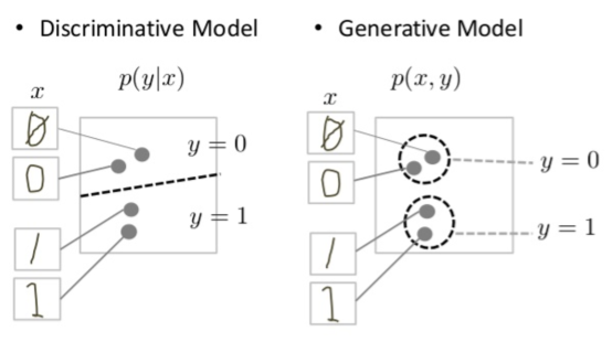
- The discriminative model tries to tell the difference between handwritten 0’s and 1’s by drawing a line in the data space. If it gets the line right, it can distinguish 0’s from 1’s without ever having to model exactly where the instances are placed in the data space on either side of the line.
- In contrast, the generative model tries to produce convincing 1’s and 0’s by generating digits that fall close to their real counterparts in the data space. It has to model the distribution throughout the data space.
- GANs offer an effective way to train such rich models to resemble a real distribution.
Overview of GAN Structure
- A generative adversarial network (GAN) has two parts:
- The generator learns to generate plausible data. The generated instances become negative training examples for the discriminator.
- The discriminator learns to distinguish the generator’s fake data from real data. The discriminator penalizes the generator for producing implausible results.
- When training begins, the generator produces obviously fake data, and the discriminator quickly learns to tell that it’s fake:

- As training progresses, the generator gets closer to producing output that can fool the discriminator:

-
In the above diagram, the generated data now has a green rectangle with the number 10 in the upper left corner and a simple drawing of a face.
-
Finally, if generator training goes well, the discriminator gets worse at telling the difference between real and fake. It starts to classify fake data as real, and its accuracy decreases.

- Here’s a picture of the whole system:

- Both the generator and the discriminator are neural networks. The generator output is connected directly to the discriminator input. Through backpropagation, the discriminator’s classification provides a signal that the generator uses to update its weights.
The Generator
- The generator part of a GAN learns to create fake data by incorporating feedback from the discriminator. It learns to make the discriminator classify its output as real.
- Generator training requires tighter integration between the generator and the discriminator than discriminator training requires. The portion of the GAN that trains the generator includes:
- random input
- generator network, which transforms the random input into a data instance
- discriminator network, which classifies the generated data
- discriminator output
- generator loss, which penalizes the generator for failing to fool the discriminator
- The figure shows backpropagation in generator training:

Random Input
- Neural networks need some form of input. Normally we input data that we want to do something with, like an instance that we want to classify or make a prediction about. But what do we use as input for a network that outputs entirely new data instances?
- In its most basic form, a GAN takes random noise as its input. The generator then transforms this noise into a meaningful output. By introducing noise, we can get the GAN to produce a wide variety of data, sampling from different places in the target distribution.
- Experiments suggest that the distribution of the noise doesn’t matter much, so we can choose something that’s easy to sample from, like a uniform distribution. For convenience the space from which the noise is sampled is usually of smaller dimension than the dimensionality of the output space.
- Note that some GANs use non-random input to shape the output. See GAN Variations. Using the Discriminator to Train the Generator
- To train a neural net, we alter the net’s weights to reduce the error or loss of its output. In our GAN, however, the generator is not directly connected to the loss that we’re trying to affect. The generator feeds into the discriminator net, and the discriminator produces the output we’re trying to affect. The generator loss penalizes the generator for producing a sample that the discriminator network classifies as fake.
- This extra chunk of network must be included in backpropagation. Backpropagation adjusts each weight in the right direction by calculating the weight’s impact on the output — how the output would change if you changed the weight. But the impact of a generator weight depends on the impact of the discriminator weights it feeds into. So backpropagation starts at the output and flows back through the discriminator into the generator.
- At the same time, we don’t want the discriminator to change during generator training. Trying to hit a moving target would make a hard problem even harder for the generator.
- So we train the generator with the following procedure:
- Sample random noise.
- Produce generator output from sampled random noise.
- Get discriminator “real” or “fake” classification for generator output.
- Calculate loss from discriminator classification.
- Backpropagate through both the discriminator and generator to obtain gradients.
- Use gradients to change only the generator weights.
- This is one iteration of generator training. In the next section we’ll see how to juggle the training of both the generator and the discriminator.
The Discriminator
- The discriminator in a GAN is simply a classifier. It tries to distinguish real data from the data created by the generator. It could use any network architecture appropriate to the type of data it’s classifying.
- The figure shows backpropagation in discriminator training:

Discriminator Training Data
-
The discriminator’s training data comes from two sources:
- Real data instances, such as real pictures of people. The discriminator uses these instances as positive examples during training.
- Fake data instances created by the generator. The discriminator uses these instances as negative examples during training.
- In the above figure, the two “Sample” boxes represent these two data sources feeding into the discriminator. During discriminator training the generator does not train. Its weights remain constant while it produces examples for the discriminator to train on.
Training the Discriminator
- The discriminator connects to two loss functions. During discriminator training, the discriminator ignores the generator loss and just uses the discriminator loss. We use the generator loss during generator training, as described in the section on Loss Functions.
- During discriminator training:
- The discriminator classifies both real data and fake data from the generator.
- The discriminator loss penalizes the discriminator for misclassifying a real instance as fake or a fake instance as real.
- The discriminator updates its weights through backpropagation from the discriminator loss through the discriminator network.
- In the next section we’ll see why the generator loss connects to the discriminator.
GAN Training
- Because a GAN contains two separately trained networks, its training algorithm must address two complications:
- GANs must juggle two different kinds of training (generator and discriminator).
- GAN convergence is hard to identify.
Alternating Training
- The generator and the discriminator have different training processes. So how do we train the GAN as a whole?
- GAN training proceeds in alternating periods:
- The discriminator trains for one or more epochs.
- The generator trains for one or more epochs.
- Repeat steps 1 and 2 to continue to train the generator and discriminator networks.
- We keep the generator constant during the discriminator training phase. As discriminator training tries to figure out how to distinguish real data from fake, it has to learn how to recognize the generator’s flaws. That’s a different problem for a thoroughly trained generator than it is for an untrained generator that produces random output.
- Similarly, we keep the discriminator constant during the generator training phase. Otherwise the generator would be trying to hit a moving target and might never converge.
- It’s this back and forth that allows GANs to tackle otherwise intractable generative problems. We get a toehold in the difficult generative problem by starting with a much simpler classification problem. Conversely, if you can’t train a classifier to tell the difference between real and generated data even for the initial random generator output, you can’t get the GAN training started.
Convergence
- As the generator improves with training, the discriminator performance gets worse because the discriminator can’t easily tell the difference between real and fake. If the generator succeeds perfectly, then the discriminator has a 50% accuracy. In effect, the discriminator flips a coin to make its prediction.
- This progression poses a problem for convergence of the GAN as a whole: the discriminator feedback gets less meaningful over time. If the GAN continues training past the point when the discriminator is giving completely random feedback, then the generator starts to train on junk feedback, and its own quality may collapse.
- For a GAN, convergence is often a fleeting, rather than stable, state.
Loss Functions
- GANs try to replicate a probability distribution. They should therefore use loss functions that reflect the distance between the distribution of the data generated by the GAN and the distribution of the real data.
- How do you capture the difference between two distributions in GAN loss functions? This question is an area of active research, and many approaches have been proposed. We’ll address two common GAN loss functions here, both of which are implemented:
- Minimax loss: The loss function used in the paper by Goodfellow et al. that introduced GANs.
- Wasserstein loss: The default loss function for TF-GAN Estimators. First described in Learning with a Wasserstein Loss by Frogner et al. (2015).
One Loss Function or Two?
- A GAN can have two loss functions: one for generator training and one for discriminator training. How can two loss functions work together to reflect a distance measure between probability distributions?
- In the loss schemes we’ll look at here, the generator and discriminator losses derive from a single measure of distance between probability distributions. In both of these schemes, however, the generator can only affect one term in the distance measure: the term that reflects the distribution of the fake data. So during generator training we drop the other term, which reflects the distribution of the real data.
- The generator and discriminator losses look different in the end, even though they derive from a single formula.
Minimax Loss
- In the paper that introduced GANs, the generator tries to minimize the following function while the discriminator tries to maximize it:
- where,
- \(D(x)\) is the discriminator’s estimate of the probability that real data instance \(x\) is real.
- \(E_x\) is the expected value over all real data instances.
- \(G(z)\) is the generator’s output when given noise \(z\).
- \(D(G(z))\) is the discriminator’s estimate of the probability that a fake instance is real.
- \(E_z\) is the expected value over all random inputs to the generator (in effect, the expected value over all generated fake instances \(G(z)\)).
- The formula derives from the cross-entropy between the real and generated distributions.
- The generator can’t directly affect the \(log(D(x))\) term in the function, so, for the generator, minimizing the loss is equivalent to minimizing \(log(1 - D(G(z)))\).
Modified Minimax Loss
- The original GAN paper notes that the above minimax loss function can cause the GAN to get stuck in the early stages of GAN training when the discriminator’s job is very easy. The paper therefore suggests modifying the generator loss so that the generator tries to maximize log D(G(z)).
Wasserstein Loss
- Wasserstein loss serves as the default loss function of several libraries including TF-GAN.
- This loss function depends on a modification of the GAN scheme (called “Wasserstein GAN” or “WGAN”) in which the discriminator does not actually classify instances. For each instance it outputs a number. This number does not have to be less than one or greater than 0, so we can’t use 0.5 as a threshold to decide whether an instance is real or fake. Discriminator training just tries to make the output bigger for real instances than for fake instances.
- Because it can’t really discriminate between real and fake, the WGAN discriminator is actually called a “critic” instead of a “discriminator”. This distinction has theoretical importance, but for practical purposes we can treat it as an acknowledgement that the inputs to the loss functions don’t have to be probabilities.
- The loss functions themselves are deceptively simple:
- Critic Loss:
- The discriminator tries to maximize this function. In other words, it tries to maximize the difference between its output on real instances and its output on fake instances.
- Generator Loss:
- The generator tries to maximize this function. In other words, It tries to maximize the discriminator’s output for its fake instances.
- where,
- \(D(x)\) is the critic’s output for a real instance.
- \(G(z)\) is the generator’s output when given noise z.
- \(D(G(z))\) is the critic’s output for a fake instance.
- The output of critic \(D\) does not have to be between 1 and 0.
- The formulas derive from the earth mover distance between the real and generated distributions.
Requirements
- The theoretical justification for the Wasserstein GAN (or WGAN) requires that the weights throughout the GAN be clipped so that they remain within a constrained range.
Benefits
- Wasserstein GANs are less vulnerable to getting stuck than minimax-based GANs, and avoid problems with vanishing gradients. The earth mover distance also has the advantage of being a true metric: a measure of distance in a space of probability distributions. Cross-entropy is not a metric in this sense.
Common Problems
- GANs have a number of common failure modes. All of these common problems are areas of active research. While none of these problems have been completely solved, we’ll mention some things that people have tried.
Vanishing Gradients
- Research has suggested that if your discriminator is too good, then generator training can fail due to vanishing gradients. In effect, an optimal discriminator doesn’t provide enough information for the generator to make progress.
Attempts to Remedy
- Wasserstein loss: The Wasserstein loss is designed to prevent vanishing gradients even when you train the discriminator to optimality.
- Modified minimax loss: The original GAN paper proposed a modification to minimax loss to deal with vanishing gradients.
Mode Collapse
- Usually you want your GAN to produce a wide variety of outputs. You want, for example, a different face for every random input to your face generator.
- However, if a generator produces an especially plausible output, the generator may learn to produce only that output. In fact, the generator is always trying to find the one output that seems most plausible to the discriminator.
- If the generator starts producing the same output (or a small set of outputs) over and over again, the discriminator’s best strategy is to learn to always reject that output. But if the next generation of discriminator gets stuck in a local minimum and doesn’t find the best strategy, then it’s too easy for the next generator iteration to find the most plausible output for the current discriminator.
- Each iteration of generator over-optimizes for a particular discriminator, and the discriminator never manages to learn its way out of the trap. As a result the generators rotate through a small set of output types. This form of GAN failure is called mode collapse.
Attempts to Remedy
- The following approaches try to force the generator to broaden its scope by preventing it from optimizing for a single fixed discriminator:
- Wasserstein loss: The Wasserstein loss alleviates mode collapse by letting you train the discriminator to optimality without worrying about vanishing gradients. If the discriminator doesn’t get stuck in local minima, it learns to reject the outputs that the generator stabilizes on. So the generator has to try something new.
- Unrolled GANs: Unrolled GANs use a generator loss function that incorporates not only the current discriminator’s classifications, but also the outputs of future discriminator versions. So the generator can’t over-optimize for a single discriminator.
Failure to Converge
- GANs frequently fail to converge, as discussed in the section on GAN training.
Attempts to Remedy
- Researchers have tried to use various forms of regularization to improve GAN convergence, including:
- Adding noise to discriminator inputs: See, for example, Toward Principled Methods for Training Generative Adversarial Networks.
- Penalizing discriminator weights: See, for example, Stabilizing Training of Generative Adversarial Networks through Regularization.
GAN Variations
- Researchers continue to find improved GAN techniques and new uses for GANs. Here’s a sampling of GAN variations to give you a sense of the possibilities.
Progressive GANs
- In a progressive GAN, the generator’s first layers produce very low resolution images, and subsequent layers add details. This technique allows the GAN to train more quickly than comparable non-progressive GANs, and produces higher resolution images.
- For more information see Karras et al, 2017.
Conditional GANs
- Conditional GANs train on a labeled data set and let you specify the label for each generated instance. For example, an unconditional MNIST GAN would produce random digits, while a conditional MNIST GAN would let you specify which digit the GAN should generate.
- Instead of modeling the joint probability \(P(X, Y)\), conditional GANs model the conditional probability \(P(X \mid Y)\).
- For more information about conditional GANs, see Mirza et al, 2014.
Image-to-Image Translation
- Image-to-Image translation GANs take an image as input and map it to a generated output image with different properties. For example, we can take a mask image with blob of color in the shape of a car, and the GAN can fill in the shape with photorealistic car details.
- Similarly, you can train an image-to-image GAN to take sketches of handbags and turn them into photorealistic images of handbags:
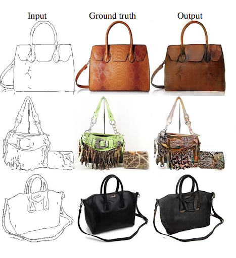
- The figure above shows a 3x3 table of pictures of handbags. Each row shows a different handbag style. In each row, the leftmost image is a simple line drawing, of a handbag, the middle image is a photo of a real handbag, and the rightmost image is a photorealistic picture generated by a GAN. The three columns are labeled ‘Input’, ‘Ground Truth’, and ‘output’.
- In these cases, the loss is a weighted combination of the usual discriminator-based loss and a pixel-wise loss that penalizes the generator for departing from the source image.
- For more information, see Isola et al, 2016.
CycleGAN
- CycleGANs learn to transform images from one set into images that could plausibly belong to another set. For example, a CycleGAN produced the righthand image below when given the lefthand image as input. It took an image of a horse and turned it into an image of a zebra. The following image shows a horse running, and a second image that’s identical in all respeccts except that the horse is a zebra:
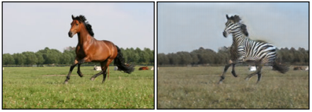
- The training data for the CycleGAN is simply two sets of images (in this case, a set of horse images and a set of zebra images). The system requires no labels or pairwise correspondences between images.
- For more information see Zhu et al, 2017, which illustrates the use of CycleGAN to perform image-to-image translation without paired data.
Text-to-Image Synthesis
- Text-to-image GANs take text as input and produce images that are plausible and described by the text. For example, the flower image below was produced by feeding a text description to a GAN.
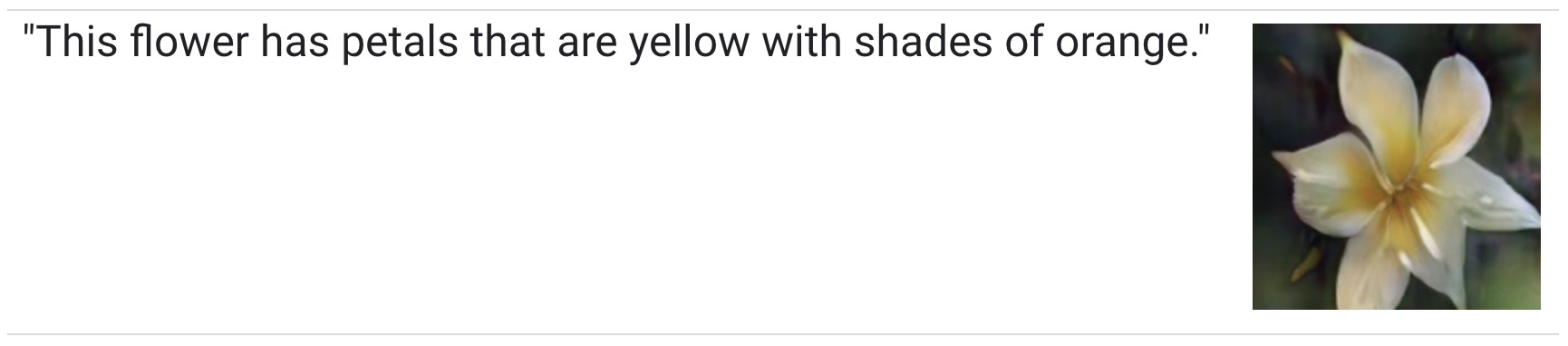
- Note that in this system the GAN can only produce images from a small set of classes.
- For more information, see Zhang et al, 2016.
Super-resolution
- Super-resolution GANs increase the resolution of images, adding detail where necessary to fill in blurry areas. For example, the blurry middle image below is a downsampled version of the original image on the left. Given the blurry image, a GAN produced the sharper image on the right:
| Original | Blurred | Restored with GAN |
|---|---|---|
 |
 |
 |
- Note that the original image shows a painting of a girl wearing an elaborate headdress. The headband of the headdress is knit in a complex pattern. Given a blurry version of the painting, a sharp, clear version is obtained at the output of the GAN.
- The GAN-generated image looks very similar to the original image, but some of the details of the patterns on her headdress and clothing are subtly different - for example, if you look closely at the headband you’ll see that the GAN didn’t reproduce the starburst pattern from the original. Instead, it made up its own plausible pattern to replace the pattern erased by the down-sampling.
- For more information, see Ledig et al, 2017.
Face Inpainting
- GANs have been used for the semantic image inpainting task. In the inpainting task, chunks of an image are blacked out, and the system tries to fill in the missing chunks.
- Yeh et al, 2017 used a GAN to outperform other techniques for inpainting images of faces. Shown below are a set of images where each image is a photo of a face with some areas replaced with black. Each image is a photo of a face identical to one of the images in the ‘Input’ column, except that there are no black areas.
| Input | GAN Output |
|---|---|
 |
 |
Text-to-Speech
- Not all GANs produce images. For example, researchers have also used GANs to produce synthesized speech from text input. For more information see Yang et al, 2017.
References
- How to Train a GAN? Tips and tricks to make GANs work by Soumith Chintala.
Citation
If you found our work useful, please cite it as:
@article{Chadha2020DistilledBERT,
  title   = {BERT},
  author  = {Chadha, Aman},
  journal = {Distilled AI},
  year    = {2020},
  note    = {\url{https://aman.ai}}
}