Primers • Double Descent
The Bias/Variance Trade-Off
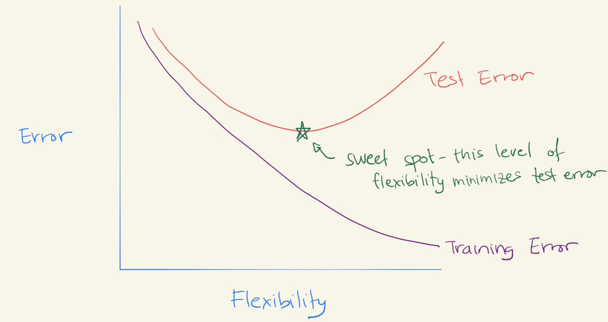
- Remember the bias/variance trade-off? It says that models perform well for an “intermediate level of flexibility”. You’ve seen the picture of the U-shape test error curve.
- We try to hit the “sweet spot” of flexibility:
- Note that this U-shape comes from the fact that
- As flexibility increases, (squared) bias decreases & variance increases. The “sweet spot” requires trading off bias and variance – i.e. a model with intermediate level of flexibility.
(Deep) Double Descent
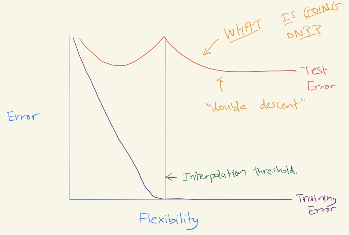
- In “Reconciling modern machine learning and the bias-variance trade-off” (2018), Belkin et al. originally noticed “double descent” – where you continue to fit increasingly flexible models that interpolate the training data, then the test error can start to decrease again.
- In “Deep Double Descent: Where Bigger Models and More Data Hurt” (2019), Nakkiran et al. show that the double descent phenomenon occurs in CNNs, ResNets, and transformers: performance first improves, then gets worse, and then improves again with increasing model size, data size, or training time. This effect can often be avoided through careful regularization. While this behavior appears to be fairly universal, we don’t yet fully understand why it happens, and view further study of this phenomenon as an important research direction.
- Check it out:
- This seems to come up in particular in the context of deep learning (though, as we’ll see, it happens elsewhere too).
- Many classes of modern deep learning models, including CNNs, ResNets, and transformers, exhibit the previously-observed double descent phenomenon when not using early stopping or regularization. The peak occurs predictably at a “critical regime,” where the models are barely able to fit the training set. As we increase the number of parameters in a neural network, the test error initially decreases, increases, and, just as the model is able to fit the train set, undergoes a second descent.
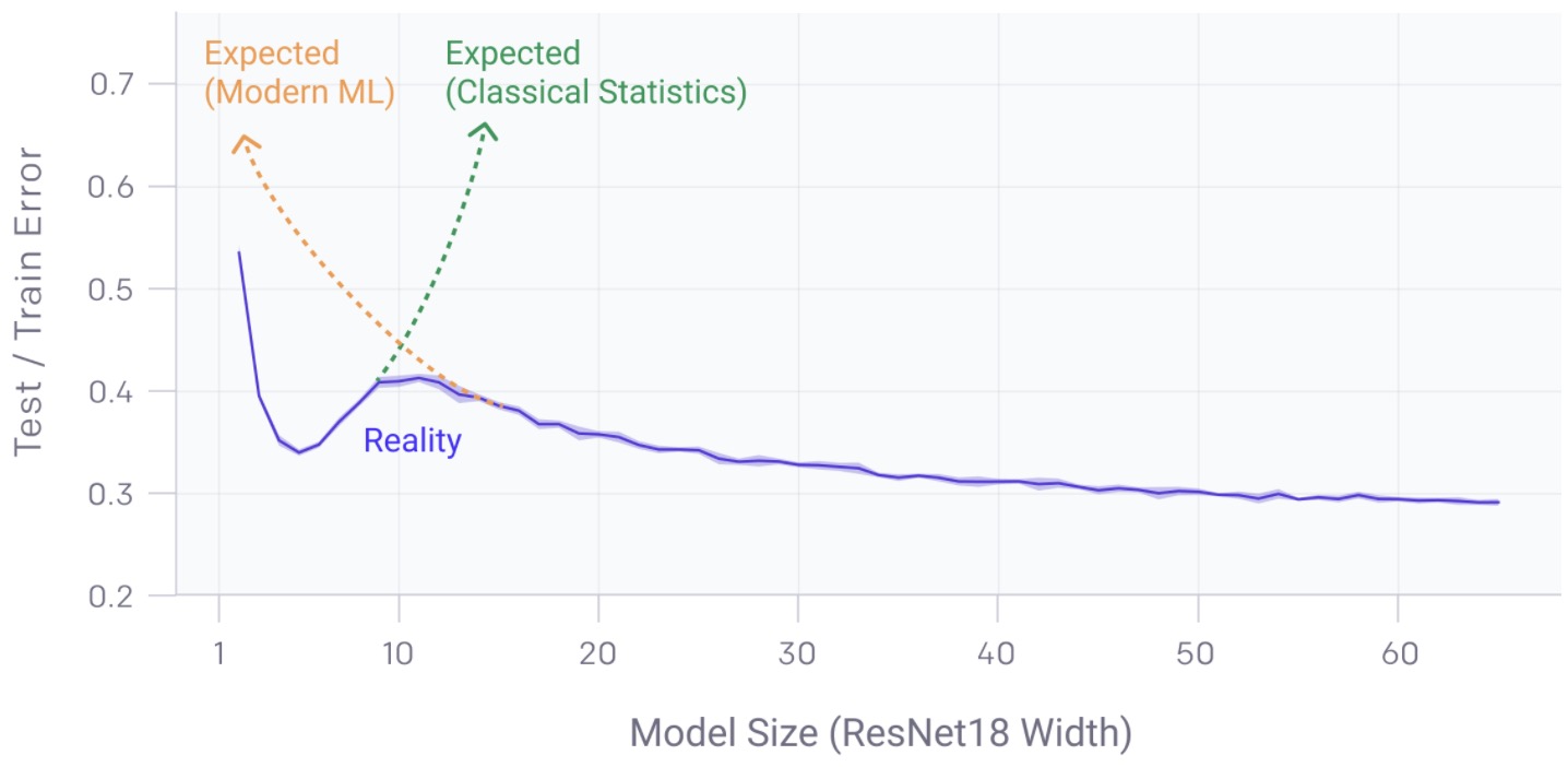
- Neither classical statisticians’ conventional wisdom that too large models are worse nor the modern ML paradigm that bigger models are better uphold. We find that double descent also occurs over train epochs. Surprisingly, we show these phenomena can lead to a regime where more data hurts, and training a deep network on a larger train set actually performs worse.
Model-wise double descent
- There is a regime where bigger models are worse, as shown in the graph below:
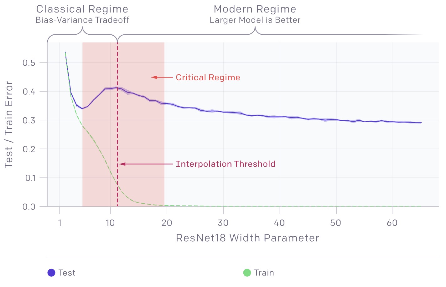
- The model-wise double descent phenomenon can lead to a regime where training on more data hurts. In the chart above, the peak in test error occurs around the interpolation threshold, when the models are just barely large enough to fit the train set.
- In all cases we’ve observed, changes which affect the interpolation threshold (such as changing the optimization algorithm, the number of train samples, or the amount of label noise) also affect the location of the test error peak correspondingly. The double descent phenomena is most prominent in settings with added label noise; without it, the peak is smaller and easy to miss. Adding label noise amplifies this general behavior and allows us to easily investigate.
Sample-wise non-monotonicity
- There is a regime where more samples hurts, as shown in the graph below:
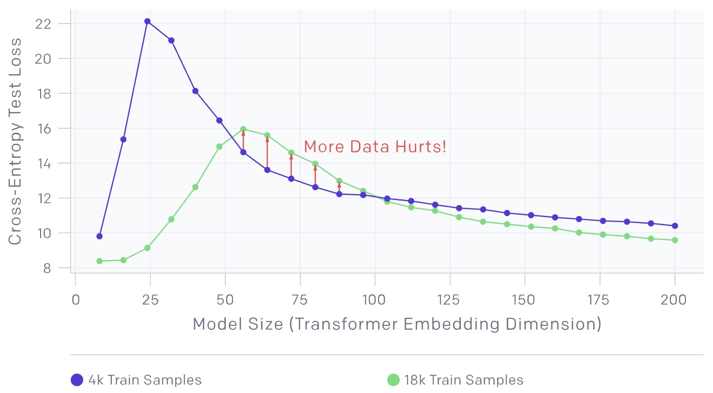
- The above chart shows transformers trained on a language-translation task with no added label noise. As expected, increasing the number of samples shifts the curve downwards towards lower test error. However, since more samples require larger models to fit, increasing the number of samples also shifts the interpolation threshold (and peak in test error) to the right.
- For intermediate model sizes (red arrows), these two effects combine, and we see that training on 4.5x more samples actually hurts test performance.
Epoch-wise double descent
- There is a regime where training longer reverses overfitting, as shown in the graphs below:
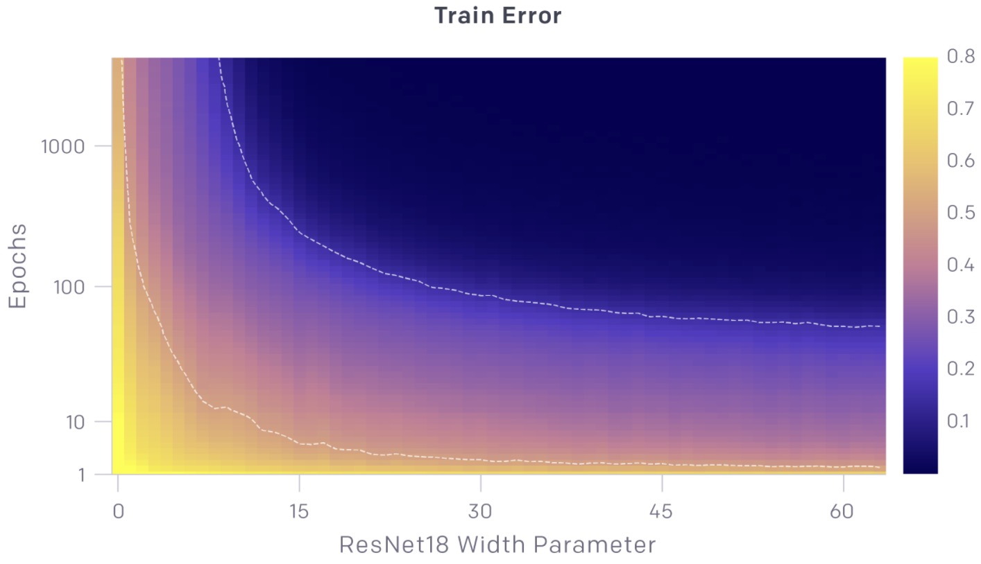
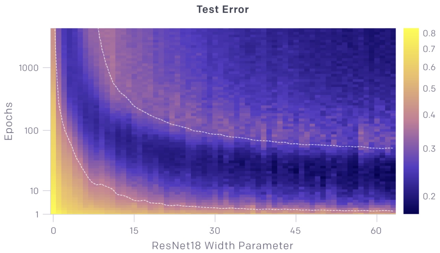
- The charts above show test and train error as a function of both model size and number of optimization steps. For a given number of optimization steps (fixed y-coordinate), test and train error exhibit model-size double descent. For a given model size (fixed x-coordinate), as training proceeds, test and train error decreases, increases, and decreases again; we call this phenomenon epoch-wise double descent.
- In general, the peak of test error appears systematically when models are just barely able to fit the train set.
- Our intuition is that, for models at the interpolation threshold, there is effectively only one model that fits the train data, and forcing it to fit even slightly noisy or misspecified labels will destroy its global structure. That is, there are no “good models” which both interpolate the train set and perform well on the test set. However, in the over-parameterized regime, there are many models that fit the train set and there exist such good models. Moreover, the implicit bias of stochastic gradient descent (SGD) leads it to such good models, for reasons we don’t yet understand.
- Nakkiran et al. (2019) leave fully understanding the mechanisms behind double descent in deep neural networks as an important open question.
Example: natural cubic splines
- To understand double descent, let’s check out a simple example that has nothing to do with deep learning: natural cubic splines. What’s a spline? Basically, it’s a way to fit the model \(Y=f(X)+\epsilon\), with \(f(\cdot)\) being non-parametric, using very smooth piecewise polynomials.
- To fit a spline, we construct some basis functions and then fit the response Y to the basis functions via least squares.
- The number of basis functions we use is the number of degrees of freedom of the spline.
- A typical basis function is given below:
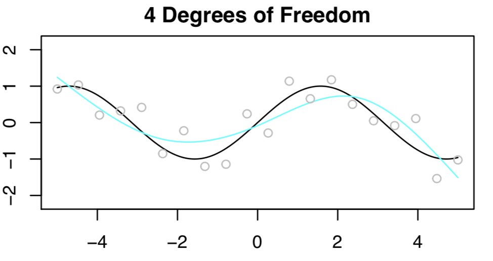
- Suppose we have \(n = 20\) (X,Y) pairs, and we want to estimate \(f(X) in Y=f(X)+\epsilon\) (here \(f(X)=\sin(X)\)) using a spline.
- First, we fit a spline with 4 DF. The \(n = 20\) observations are in gray, true function \(f(x)\) is in black, and the fitted function is in light blue. Not bad!
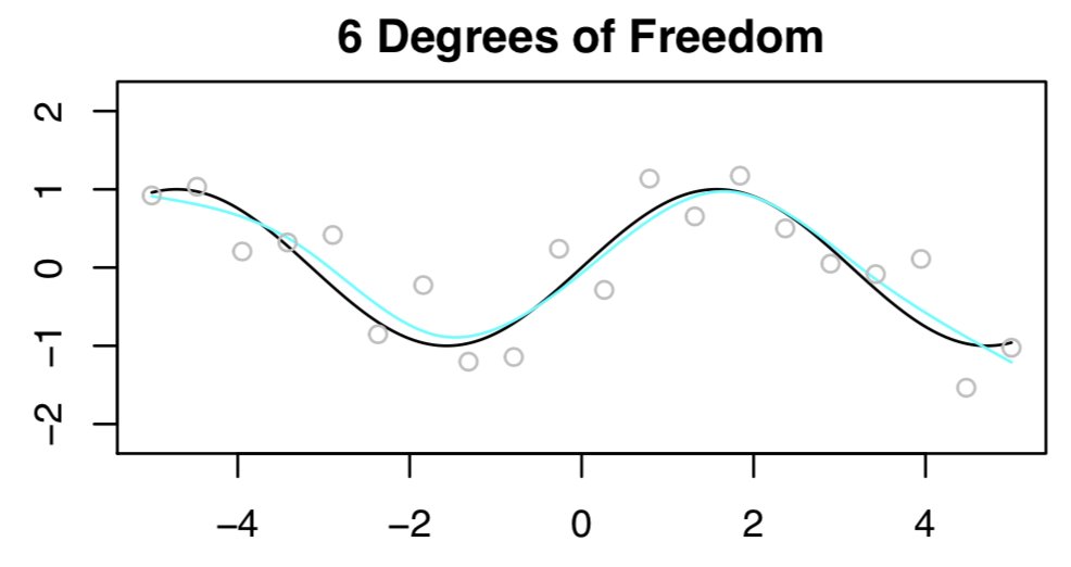
- Now let’s try again, this time with 6 degrees of freedom. This looks awesome, as shown below.
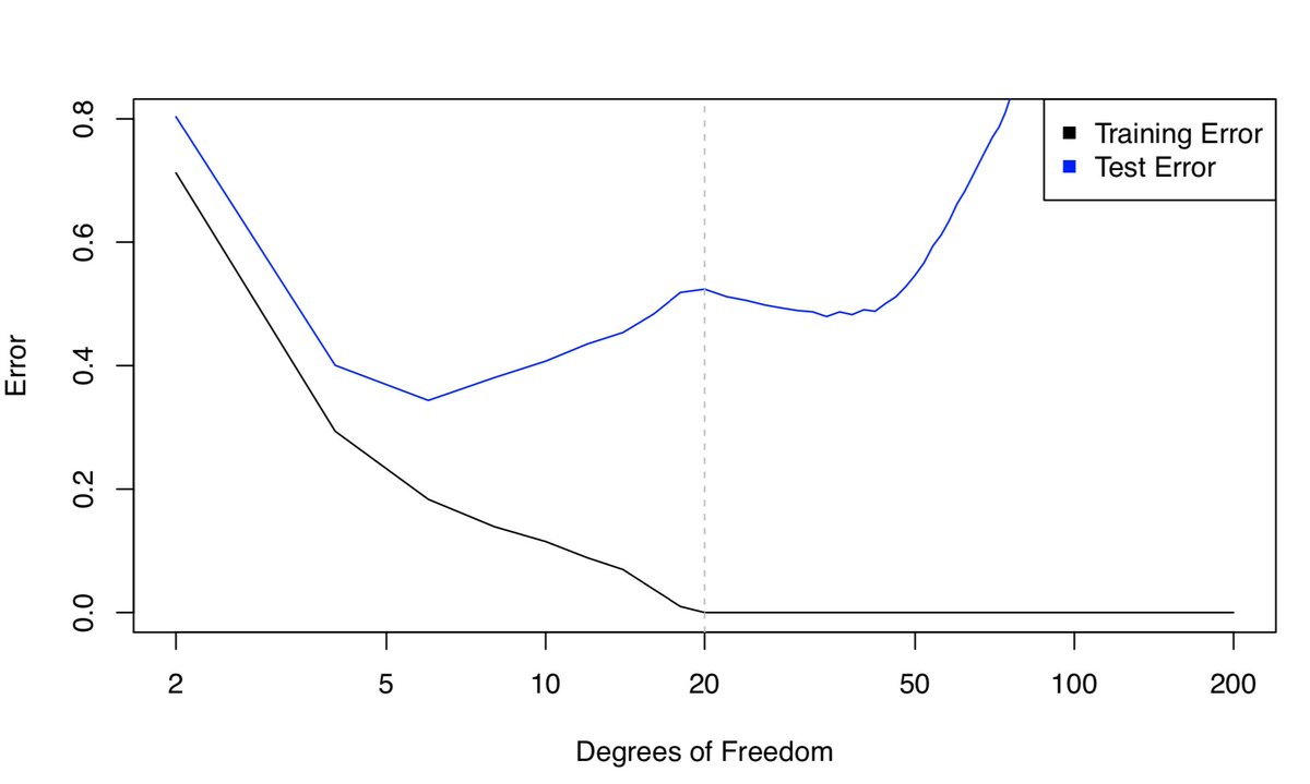
- Now what if we use 20 degrees of freedom? Intuitively, it seems like a bad idea, because we have n=20 observations and to fit a spline with 20 DF, we need to run least squares with 20 features. We’ll get zero training error (i.e. interpolate the training set) and bad test error!
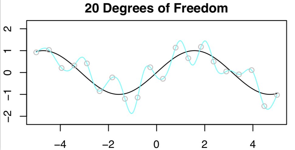
- The interpolation threshold is roughly where parameters == data points which can be seen from the results in the figure, just as the bias-variance trade-off predicts. All’s well in the world.
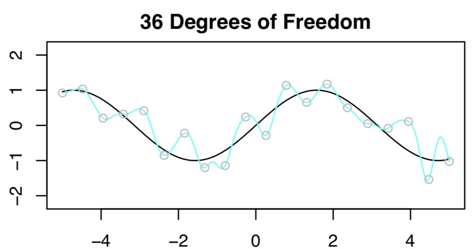
- Next, we’re trying to fit a spline using least squares with n=20 and 36 DF (i.e., \(p=36\)). With \(p>n\) the LS solution isn’t even unique!
- To select among the infinite number of solutions, let’s choose the “minimum” norm fit: the one with the smallest sum of squared coefficients. [Easy to compute using everybody’s favorite matrix decomp, the SVD.] The result is expected to be horrible, because \(p > n\). Here’s what we get:
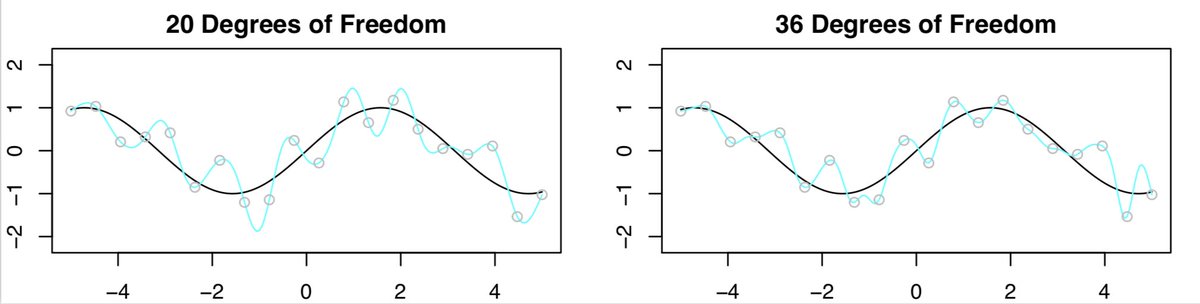
- Now, let’s compare the results with 20 DF to 36 DF. We expected the fit with 36 DF to look worse than the one with 20 DF, however, surprisingly it looks a little better!
- Upon taking a peek at the training and test error, we see that the test error (briefly) decreases when \(p > n\). However, that sounds counter intuitive since it is literally the opposite of what the bias-variance trade-off says should happen!
-
The key point is with 20 DF, n=p, and there’s exactly one least squares fit that has zero training error. And that fit happens to have oodles of wiggles, but as we increase the DF so that \(p>n\), there are tons of interpolating least squares fits.
-
The minimum norm least squares fit is the “least wiggly” of those zillions of fits. Also, note that the “least wiggly” among them is even less wiggly than the fit when \(p=n\).
-
So, “double descent” is happening because DF isn’t really the right quantity for the the X-axis: like, the fact that we are choosing the minimum norm least squares fit actually means that the spline with 36 DF is less flexible than the spline with 20 DF.
-
Now, what if had used a ridge penalty when fitting the spline (instead of least squares)? In that case, we wouldn’t have interpolated training set, we wouldn’t have seen double descent, and we would have gotten better test error (for the right value of the tuning parameter!).
-
How does this relate to deep learning? When we use (stochastic) gradient descent to fit a neural net, we are actually picking out the minimum norm solution!! So the spline example is a pretty good analogy for what is happening when we see double descent for neural nets.
-
Key takeaways
- Double descent is observed and is understandable through the lens of stat ML and the bias/variance trade-off.
- Actually, the bias/variance trade-off helps us understand why DD is happening!
References
- CS229 Notes.
- “Reconciling modern machine learning and the bias-variance trade-off” (2019) by Nakkiran et al. presents an in-depth treatment on deep double descent.
- Deep Double Descent for the overview of the paper.
- Daniela Witten’s Twitter for the awesome double descent explanation.
- “Reconciling modern machine learning and the bias-variance trade-off” (2018) by Belkin et al. is actually the original “double descent” paper.
- Yannic Kilcher’s YouTube video presents a nice visual walkthrough of the paper.
Citation
If you found our work useful, please cite it as:
@article{Chadha2020DistilledDoubleDescent,
  title   = {Double Descent},
  author  = {Chadha, Aman},
  journal = {Distilled AI},
  year    = {2020},
  note    = {\url{https://aman.ai}}
}