Primers • Distributed Training Parallelism
- Background
- Overview: Types of Parallelism
- Data Parallelism
- Model Parallelism
- Hybrid (Model and Data) Parallelism
- Tensor Parallelism
- Pipeline Parallelism
- Comparative Analysis: DP, DDP, FSDP, DeepSpeed, and DeepSpeed ZeRO
- Further Reading
- Citation
Background
- Distributed training parallelism is crucial for efficiently training large-scale deep learning models that require extensive computational resources. This approach leverages multiple GPUs or machines to perform computations in parallel, significantly reducing training time and enabling the handling of larger datasets and models.
- There are four main strategies for parallelism in distributed training: model, data, pipeline, and tensor parallelism. Each has its own mechanisms, advantages, and challenges, and understanding them is essential for optimizing training performance in different scenarios.
Overview: Types of Parallelism
Model Parallelism
- Model parallelism is a strategy for distributing the computation of a deep learning model across multiple GPUs or other computing devices. This approach is particularly beneficial when the model is too large to fit into the memory of a single GPU. Instead of duplicating the entire model on each GPU (as in data parallelism), different parts of the model are placed on different GPUs, allowing for the training of very large models.
Concept
- In model parallelism, the model is partitioned such that each GPU is responsible for a subset of the model parameters. During the forward pass, data flows through these partitions sequentially, with intermediate results transferred between GPUs as needed. The backward pass similarly computes gradients for each partition, which are then used to update the parameters locally on each GPU.
Mechanism
- Model Partitioning:
- The model is divided into distinct segments, each assigned to a different GPU. For example, in a neural network, different layers or groups of layers might be placed on different GPUs.
- Forward Pass:
- Input data is fed into the first segment of the model on the first GPU. The output of this segment is transferred to the next GPU, which processes the next segment of the model, and so on until the final segment.
- Backward Pass:
- During backpropagation, gradients are computed in the reverse order. Each GPU computes the gradients for its segment and passes the necessary information back to the previous GPU to continue the gradient computation.
- Parameter Update:
- Each GPU updates the parameters of its segment locally. If needed, synchronization steps can ensure consistency across GPUs.
Pros and Cons
- Pros:
- Memory Efficiency: Allows for training models that are too large to fit into the memory of a single GPU by distributing the model’s parameters and intermediate activations across multiple GPUs.
- Scalability: Enables the use of large-scale models in research and production, leveraging multiple GPUs to handle complex computations.
- Resource Utilization: Can optimize the utilization of available computational resources by balancing the load across multiple GPUs.
- Cons:
- Complexity: Implementing model parallelism can be challenging due to the need to carefully manage data transfers and dependencies between different parts of the model.
- Communication Overhead: Transferring intermediate results between GPUs introduces latency, which can become a bottleneck, especially if the network bandwidth is limited.
- Synchronization Issues: Ensuring that all parts of the model remain synchronized during training can be difficult, particularly in distributed environments.
Use Cases
- Model parallelism is especially useful in scenarios where the model size exceeds the memory capacity of a single GPU. Some common use cases include:
- Large Language Models: Models like GPT-3, which have billions of parameters, often require model parallelism to be trained effectively.
- Deep Convolutional Networks: Very deep networks with many layers can benefit from model parallelism by distributing layers across multiple GPUs.
- 3D Convolutional Networks: Used in applications like video processing and 3D object recognition, where the model size can be substantial.
Implementation in PyTorch
- In PyTorch, model parallelism can be implemented by manually assigning different parts of the model to different GPUs. Here’s a basic example:
import torch
import torch.nn as nn
import torch.optim as optim

# Define a simple model with two linear layers
class SimpleModel(nn.Module):
    def __init__(self):
        super(SimpleModel, self).__init__()
        self.layer1 = nn.Linear(10, 10).to('cuda:0')  # Place on GPU 0
        self.layer2 = nn.Linear(10, 10).to('cuda:1')  # Place on GPU 1

    def forward(self, x):
        x = self.layer1(x)
        x = x.to('cuda:1')  # Move intermediate output to GPU 1
        x = self.layer2(x)
        return x

# Initialize model, loss, and optimizer
model = SimpleModel()
criterion = nn.MSELoss()
optimizer = optim.SGD(model.parameters(), lr=0.01)

# Dummy input and target
input_data = torch.randn(5, 10).to('cuda:0')
target = torch.randn(5, 10).to('cuda:1')

# Forward pass
output = model(input_data)
loss = criterion(output, target)

# Backward pass
loss.backward()

# Optimizer step
optimizer.step()
- In this example, the model has two linear layers, each placed on a different GPU. During the forward pass, the input is moved between GPUs as needed. The backward pass and optimizer step handle the parameter updates for each layer separately.
Conclusion
- Model parallelism is a powerful technique for training large models that cannot fit into the memory of a single GPU. While it introduces complexity in terms of implementation and communication overhead, it enables the training of state-of-the-art models in various fields, from natural language processing to computer vision. Properly balancing the model segments and managing the data flow are key challenges, but with frameworks like PyTorch providing the necessary tools, model parallelism can be effectively leveraged to push the boundaries of deep learning research and applications.
Summary
- Concept:
- Model parallelism involves splitting the model itself across multiple GPUs. Different layers or parts of the model are assigned to different GPUs. This is particularly useful when a model is too large to fit into the memory of a single GPU.
- Mechanism:
- Data flows sequentially through the model parts across different GPUs.
- Each GPU computes its assigned part of the forward and backward passes.
- Pros:
- Enables training of very large models that do not fit into a single GPU’s memory.
- Can optimize memory usage and computational load distribution.
- Cons:
- More complex to implement due to the need to manage dependencies and data transfers between GPUs.
- May introduce latency due to data transfer between GPUs.
Data Parallelism
- Data parallelism is a technique in parallel computing where data is distributed across multiple processors or machines, and each processor performs the same operation on different parts of the data simultaneously. This approach is particularly effective in scenarios where the same set of operations need to be applied to large datasets.
Concept
- The fundamental concept of data parallelism is to break down a large dataset into smaller chunks and process these chunks in parallel. Each processor (or core) receives a portion of the data and applies the same computational operations. After processing, the results are aggregated to form the final output.
Mechanism
-
Data Splitting: The dataset is divided into smaller, equally-sized chunks. Each chunk is assigned to a different processor or computing unit.
-
Parallel Execution: Each processor performs the same operation on its assigned chunk of data. This step happens concurrently, leveraging the parallel nature of the computing environment.
-
Synchronization: After processing, the results from each processor are synchronized. This step may involve combining or aggregating the processed data to produce the final result.
-
Result Aggregation: The partial results from each processor are combined to form the complete output. This step may require communication between processors to gather and combine the data.
Pros and Cons
Pros:
- Increased Efficiency: By processing data in parallel, the overall computational time is reduced significantly.
- Scalability: Data parallelism can scale with the number of processors, making it suitable for large-scale data processing tasks.
- Resource Utilization: Efficiently utilizes available computing resources by distributing the workload.
Cons:
- Communication Overhead: Synchronizing and aggregating results can introduce overhead, especially in distributed systems.
- Complexity: Implementing data parallelism can be complex, requiring careful management of data distribution and synchronization.
- Limited by Data Size: The size of the dataset must be sufficiently large to justify the overhead of parallelization.
Use Cases
- Deep Learning: Training large neural networks where massive datasets are divided and processed in parallel across multiple GPUs.
- Big Data Analytics: Processing large volumes of data in parallel to extract insights and perform analytics.
- Scientific Simulations: Running simulations that require processing large datasets, such as weather forecasting or molecular dynamics.
Implementation in PyTorch
- PyTorch provides several utilities to implement data parallelism easily:
-
torch.nn.DataParallel: A simple way to wrap a model to enable parallel processing across multiple GPUs.import torch import torch.nn as nn import torch.optim as optim # Define the model model = nn.DataParallel(MyModel()) # Move the model to GPU model.to('cuda') # Define the optimizer and loss function optimizer = optim.SGD(model.parameters(), lr=0.01) criterion = nn.CrossEntropyLoss() # Training loop for data, target in dataloader: data, target = data.to('cuda'), target.to('cuda') optimizer.zero_grad() output = model(data) loss = criterion(output, target) loss.backward() optimizer.step() -
Distributed Data Parallel (DDP): For more advanced and scalable parallelism, PyTorch offers
torch.nn.parallel.DistributedDataParallel. This approach is more efficient and scalable for large-scale applications.import torch import torch.distributed as dist import torch.multiprocessing as mp from torch.nn.parallel import DistributedDataParallel as DDP def train(rank, world_size): # Initialize the process group dist.init_process_group("gloo", rank=rank, world_size=world_size) # Create model and move it to GPU with rank model = MyModel().to(rank) ddp_model = DDP(model, device_ids=[rank]) # Define loss function and optimizer loss_fn = nn.CrossEntropyLoss() optimizer = optim.SGD(ddp_model.parameters(), lr=0.01) # Training loop for data, target in dataloader: data, target = data.to(rank), target.to(rank) optimizer.zero_grad() outputs = ddp_model(data) loss = loss_fn(outputs, target) loss.backward() optimizer.step() # Clean up dist.destroy_process_group() def main(): world_size = 4 mp.spawn(train, args=(world_size,), nprocs=world_size, join=True) if __name__ == "__main__": main()
Conclusion
- Data parallelism is a powerful technique to enhance computational efficiency by distributing data across multiple processors or machines. It is highly beneficial in scenarios involving large datasets and complex computations, such as deep learning and big data analytics. While data parallelism offers significant advantages in terms of speed and scalability, it also introduces challenges like communication overhead and implementation complexity. PyTorch provides robust tools for implementing data parallelism, making it accessible for both simple and advanced use cases.
Summary
- Concept:
- Data parallelism involves splitting the dataset into smaller batches and distributing these batches across multiple GPUs. Each GPU holds a complete copy of the model and processes a subset of the data independently. After computation, the results (such as gradients) are synchronized and aggregated to update the model parameters.
- Mechanism:
- Each GPU computes the forward and backward passes for its portion of the data.
- Gradients are averaged across all GPUs.
- Model parameters are updated synchronously to ensure all GPUs have identical parameters.
- Pros:
- Easy to implement and highly effective for many types of models.
- Scales well with the number of GPUs.
- Cons:
- Limited by the memory of a single GPU, as each GPU must hold the entire model.
- Communication overhead during synchronization can become a bottleneck.
Pipeline Parallelism
- Concept:
- Pipeline parallelism is a specific form of model parallelism where different stages of the model are distributed across multiple GPUs. The model is divided into stages, and data is processed in a pipeline fashion, allowing different GPUs to work on different mini-batches of data simultaneously.
- Mechanism:
- The model is split into several stages, each assigned to a different GPU.
- Mini-batches are divided into micro-batches and fed sequentially through the stages.
-
While one GPU is processing a micro-batch, another GPU can start processing the next micro-batch.
- Pros:
- Reduces idle time by overlapping computation and communication.
- Effective for deep models with many sequential layers.
- Cons:
- Introduces pipeline bubbles (idle time) at the start and end of the pipeline.
- Requires careful tuning to balance the stages and manage the pipeline efficiently.
Tensor Parallelism
- Concept:
- Tensor parallelism involves splitting individual tensors (such as weight matrices) across multiple GPUs. This approach allows large tensors to be distributed and processed in parallel, effectively balancing the computation load.
- Mechanism:
- Tensors are divided along one or more dimensions, and each GPU holds a slice of the tensor.
- During computation, operations are performed on these slices in parallel, and the results are combined as needed.
- Pros:
- Can handle extremely large tensors that exceed the memory capacity of a single GPU.
- Distributes computational load more evenly across GPUs.
- Cons:
- Requires sophisticated implementation to manage tensor slicing and the corresponding operations.
- Communication overhead for combining the results can impact performance.
Choosing the right strategy: Data v/s Model v/s Pipeline v/s Tensor Parallelism
-
Each parallelism paradigm offers unique advantages and is suitable for different scenarios:
- Data Parallelism is simple and effective for many models but limited by GPU memory constraints.
- Model Parallelism allows for training very large models but requires careful management of data flow between GPUs.
- Pipeline Parallelism optimizes utilization by overlapping computations but introduces complexity in balancing the pipeline.
- Tensor Parallelism handles extremely large tensors efficiently but involves intricate implementation and communication overhead.
- Choosing the right parallelism strategy depends on the specific requirements of the model, the hardware architecture, and the desired performance characteristics.
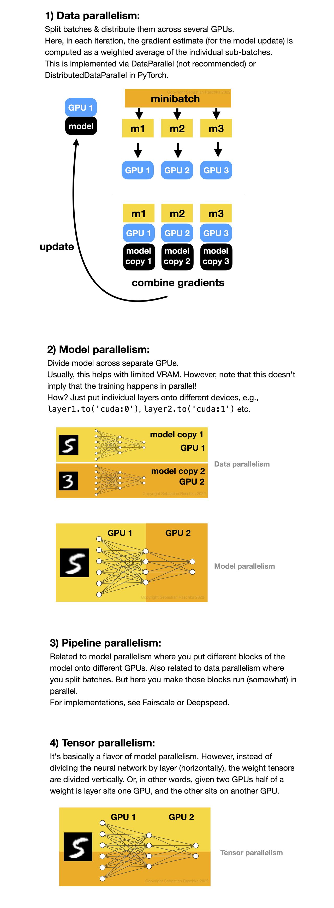
- The infographic below (credits to Sebastian Raschka) offers a quick overview of the four different paradigms for multi-GPU training, such as data parallelism, model parallelism, pipeline parallelism, and tensor parallelism.
Data Parallelism
- Data parallelism involves splitting the data across multiple devices (such as GPUs). Each device processes a different chunk of the data, but they all use the same model to perform computations. After processing, the results are combined to update the model. This is accomplished by synchronizing the gradients during the backward pass to ensure consistent updates.
DataParallel (DP)
- Data parallelism in PyTorch refers to the process of distributing data across multiple GPUs to perform parallel computations. This approach helps to accelerate training by utilizing the computational power of multiple GPUs simultaneously. The primary mechanism for achieving data parallelism in PyTorch is through the
torch.nn.DataParallelmodule. - Here’s a detailed explanation of how
torch.nn.DataParallelworks and a small code sample to demonstrate its usage.
How DP Works
- Model Replication: The model is replicated across multiple GPUs, with each replica handling a portion of the input data.
- Data Splitting: The input data is split into smaller batches, and each smaller batch is sent to a different GPU.
- Parallel Computation: Each GPU processes its portion of the data in parallel, performing forward and backward passes independently.
- Gradient Aggregation: Gradients from all GPUs are gathered and averaged.
- Model Update: The averaged gradients are used to update the model parameters.
Key Steps in Using DP
- Model Definition: Define the model as usual.
- Wrap with DataParallel: Use
torch.nn.DataParallelto wrap the model. - Data Loading: Use
torch.utils.data.DataLoaderto load the dataset. - Forward and Backward Pass: Perform the forward and backward pass in the same way as with a single GPU, but now the computations will be distributed across multiple GPUs.
Code Sample
import torch
import torch.nn as nn
import torch.optim as optim
from torchvision import datasets, transforms

# Define a simple CNN model
class SimpleCNN(nn.Module):
    def __init__(self):
        super(SimpleCNN, self).__init__()
        self.conv1 = nn.Conv2d(1, 32, kernel_size=3, stride=1, padding=1)
        self.conv2 = nn.Conv2d(32, 64, kernel_size=3, stride=1, padding=1)
        self.fc1 = nn.Linear(64 * 28 * 28, 128)
        self.fc2 = nn.Linear(128, 10)

    def forward(self, x):
        x = nn.functional.relu(self.conv1(x))
        x = nn.functional.relu(self.conv2(x))
        x = x.view(-1, 64 * 28 * 28)
        x = nn.functional.relu(self.fc1(x))
        x = self.fc2(x)
        return x

# Check if multiple GPUs are available
device = torch.device("cuda" if torch.cuda.is_available() else "cpu")
print(f"Using device: {device}")

# Instantiate the model
model = SimpleCNN()

# Wrap the model with DataParallel
if torch.cuda.device_count() > 1:
    print(f"Using {torch.cuda.device_count()} GPUs")
    model = nn.DataParallel(model)

# Move the model to the appropriate device
model.to(device)

# Define a loss function and optimizer
criterion = nn.CrossEntropyLoss()
optimizer = optim.Adam(model.parameters(), lr=0.001)

# Data loading and preprocessing
transform = transforms.Compose([
    transforms.ToTensor(),
    transforms.Normalize((0.1307,), (0.3081,))
])

train_dataset = datasets.MNIST(root='./data', train=True, download=True, transform=transform)
train_loader = torch.utils.data.DataLoader(dataset=train_dataset, batch_size=64, shuffle=True)

# Training loop
for epoch in range(5):
    model.train()
    running_loss = 0.0
    for i, (inputs, labels) in enumerate(train_loader):
        inputs, labels = inputs.to(device), labels.to(device)

        optimizer.zero_grad()
        outputs = model(inputs)
        loss = criterion(outputs, labels)
        loss.backward()
        optimizer.step()

        running_loss += loss.item()
        if i % 100 == 99:    # Print every 100 mini-batches
            print(f'Epoch [{epoch + 1}, {i + 1}] loss: {running_loss / 100:.3f}')
            running_loss = 0.0

print('Training finished.')
Explanation of the Code
- Model Definition: A simple CNN model is defined.
- Device Check: The code checks if CUDA is available and sets the appropriate device.
- Model Wrapping: The model is wrapped with
torch.nn.DataParallelif multiple GPUs are available. - Data Loading: The MNIST dataset is loaded and transformed.
- Training Loop: The model is trained in the usual way, but the computations are distributed across multiple GPUs if available.
Distributed Data Parallel (DDP)
- By using
torch.nn.DataParallel, you can easily scale your model training to utilize multiple GPUs, which can significantly speed up the training process. - Distributed Data Parallel (DDP) in PyTorch is a more advanced and efficient method for parallelizing training across multiple GPUs, potentially across multiple nodes. Unlike
torch.nn.DataParallel, which uses a single process to manage all devices, DDP creates a separate process for each GPU, allowing for better scalability and reduced inter-GPU communication overhead. This approach is particularly beneficial for large-scale deep learning tasks.
Key Features of DDP
- Separate Processes: Each GPU is managed by a separate process, which helps in minimizing the bottleneck caused by the Global Interpreter Lock (GIL) in Python.
- Gradient Synchronization: Gradients are synchronized across processes using an all-reduce operation, ensuring that all processes have consistent model parameters.
- Scalability: Better performance and scalability compared to
torch.nn.DataParallel, especially for large-scale training.
Technical Steps to Use DDP
- Initialize the Process Group: Set up the communication backend and initialize the process group.
- Create DDP Model: Wrap the model with
torch.nn.parallel.DistributedDataParallel. - Set Up Distributed Sampler: Use a distributed sampler to ensure each process gets a unique subset of the dataset.
- Configure Data Loaders: Set up data loaders with the distributed sampler.
- Launch Training Processes: Use a launcher utility to spawn multiple processes for training.
Code Sample
- Here’s a basic example demonstrating how to set up and use DDP in PyTorch.
import os
import torch
import torch.distributed as dist
import torch.multiprocessing as mp
from torch.nn.parallel import DistributedDataParallel as DDP
from torchvision import datasets, transforms
from torch.utils.data import DataLoader, DistributedSampler
import torch.nn as nn
import torch.optim as optim

def setup(rank, world_size):
    os.environ['MASTER_ADDR'] = 'localhost'
    os.environ['MASTER_PORT'] = '12355'
    dist.init_process_group("nccl", rank=rank, world_size=world_size)

def cleanup():
    dist.destroy_process_group()

class SimpleCNN(nn.Module):
    def __init__(self):
        super(SimpleCNN, self).__init__()
        self.conv1 = nn.Conv2d(1, 32, kernel_size=3, stride=1, padding=1)
        self.conv2 = nn.Conv2d(32, 64, kernel_size=3, stride=1, padding=1)
        self.fc1 = nn.Linear(64 * 28 * 28, 128)
        self.fc2 = nn.Linear(128, 10)

    def forward(self, x):
        x = nn.functional.relu(self.conv1(x))
        x = nn.functional.relu(self.conv2(x))
        x = x.view(-1, 64 * 28 * 28)
        x = nn.functional.relu(self.fc1(x))
        x = self.fc2(x)
        return x

def train(rank, world_size, epochs):
    setup(rank, world_size)

    transform = transforms.Compose([
        transforms.ToTensor(),
        transforms.Normalize((0.1307,), (0.3081,))
    ])

    train_dataset = datasets.MNIST(root='./data', train=True, download=True, transform=transform)
    train_sampler = DistributedSampler(train_dataset, num_replicas=world_size, rank=rank)
    train_loader = DataLoader(dataset=train_dataset, batch_size=64, sampler=train_sampler)

    model = SimpleCNN().to(rank)
    model = DDP(model, device_ids=[rank])

    criterion = nn.CrossEntropyLoss().to(rank)
    optimizer = optim.Adam(model.parameters(), lr=0.001)

    for epoch in range(epochs):
        model.train()
        running_loss = 0.0
        for i, (inputs, labels) in enumerate(train_loader):
            inputs, labels = inputs.to(rank), labels.to(rank)

            optimizer.zero_grad()
            outputs = model(inputs)
            loss = criterion(outputs, labels)
            loss.backward()
            optimizer.step()

            running_loss += loss.item()
            if i % 100 == 99:
                print(f'Rank {rank}, Epoch [{epoch + 1}, {i + 1}] loss: {running_loss / 100:.3f}')
                running_loss = 0.0

    cleanup()

def main():
    world_size = torch.cuda.device_count()
    epochs = 5
    mp.spawn(train, args=(world_size, epochs), nprocs=world_size, join=True)

if __name__ == "__main__":
    main()
Explanation of the Code
- Setup and Cleanup: Functions to initialize and destroy the process group.
- Model Definition: A simple CNN model is defined.
- Train Function:
- Initializes the process group.
- Creates a distributed sampler and data loader.
- Wraps the model with
DistributedDataParallel. - Runs the training loop.
- Main Function: Uses
mp.spawnto launch multiple processes for training.
- This setup ensures that each GPU gets its own process and subset of the data, with gradients synchronized across processes, allowing for efficient parallel training.
Model Parallelism
- Model parallelism involves splitting the neural network model across multiple devices (such as GPUs) so that each device is responsible for a part of the model. This approach is particularly useful when the model is too large to fit into the memory of a single device. By distributing different parts of the model across multiple GPUs, model parallelism enables the training of very large models.
- Types of Model Parallelism:
- Layer-wise Parallelism
- Tensor-wise Parallelism
- Operator-wise Parallelism
Layer-wise Parallelism
- Concept:
- Different layers or groups of layers of the model are assigned to different GPUs. For example, in a deep neural network, you might place the first few layers on one GPU, the next few layers on another GPU, and so on.
- Mechanism:
- During the forward pass, the output of one GPU is transferred to the next GPU for further processing.
- During the backward pass, gradients are computed in the reverse order, with each GPU handling the gradients for its assigned layers.
- Pros:
- Simple to implement for sequential models.
- Good for models with distinct layers or blocks.
- Cons:
- Can lead to inefficient GPU utilization if layers have varying computational loads.
- Communication overhead can be significant if layers produce large outputs.
- Example:
import torch
import torch.nn as nn

class LayerwiseModel(nn.Module):
    def __init__(self):
        super(LayerwiseModel, self).__init__()
        self.layer1 = nn.Linear(10, 50).to('cuda:0')
        self.layer2 = nn.Linear(50, 10).to('cuda:1')

    def forward(self, x):
        x = self.layer1(x)
        x = x.to('cuda:1')
        x = self.layer2(x)
        return x
Tensor-wise Parallelism
- Concept:
- Individual tensors, such as weight matrices or activations, are split across multiple GPUs. This approach involves slicing tensors along one or more dimensions and distributing these slices across different GPUs.
- Mechanism:
- During computation, each GPU processes its slice of the tensor in parallel.
- Intermediate results are combined as needed to complete the computation.
- Pros:
- Efficiently utilizes GPU memory by distributing large tensors.
- Balances computational load more evenly across GPUs.
- Cons:
- Requires sophisticated implementation to handle tensor slicing and combining.
- High communication overhead for combining intermediate results.
- Example:
- Tensor-wise parallelism is often implemented at a lower level within deep learning frameworks and may not be directly visible in user-defined model code. It’s commonly used in distributed training libraries like Megatron-LM for large-scale models.
Operator-wise Parallelism
- Concept:
- Different operations (or parts of operations) within a layer are assigned to different GPUs. This fine-grained parallelism involves splitting the computation of individual operations across multiple devices.
- Mechanism:
- Operations within a layer are divided, with each GPU performing a portion of the computation.
- Results from each GPU are combined to produce the final output of the operation.
- Pros:
- Can achieve high parallel efficiency by leveraging all available GPUs.
- Useful for very large operations that can be broken down into smaller, parallelizable tasks.
- Cons:
- Complex to implement and manage.
- Communication overhead can be significant, particularly for operations with large intermediate results.
- Example:
- Similar to tensor-wise parallelism, operator-wise parallelism is usually implemented within deep learning libraries and frameworks, optimizing specific operations like matrix multiplications.
Summary
-
Model parallelism can be categorized into three main types, each suited to different scenarios and offering unique advantages and challenges:
- Layer-wise Parallelism: Simple to implement and effective for models with clear layer separations but may lead to imbalanced GPU utilization and communication overhead.
- Tensor-wise Parallelism: Efficiently uses GPU memory and balances computational load by splitting large tensors but requires sophisticated slicing and communication management.
- Operator-wise Parallelism: Maximizes parallel efficiency by splitting operations within layers but is complex to implement and can incur significant communication overhead.
-
Choosing the appropriate type of model parallelism depends on the model architecture, the available hardware, and the specific requirements of the training task. Advanced deep learning frameworks and libraries provide tools and functionalities to facilitate the implementation of these parallelism strategies, enabling the training of large and complex models.
Comparative Analysis: Types of Model Parallelism
Criteria for Comparison
- Implementation Complexity
- GPU Utilization
- Communication Overhead
- Scalability
- Suitable Use Cases
Layer-wise Parallelism
- Implementation Complexity:
- Low to Medium: It’s relatively straightforward to assign different layers or groups of layers to different GPUs. This method is particularly simple for models with a clear sequential structure.
- GPU Utilization:
- Variable: The utilization can be uneven if different layers have varying computational loads. Some GPUs may be underutilized while waiting for others to complete their tasks.
- Communication Overhead:
- High: Significant overhead can arise from transferring large intermediate results between GPUs. This can be a bottleneck, especially with deep models producing large outputs.
- Scalability:
- Moderate: Scalability is limited by the number of layers that can be effectively divided among GPUs. Deep models with many layers can benefit, but shallow models may not.
- Suitable Use Cases:
- Sequential models with distinct layers, such as feedforward neural networks or deep convolutional networks.
Tensor-wise Parallelism
- Implementation Complexity:
- High: Requires advanced techniques to split and manage tensors across multiple GPUs. It involves slicing tensors along specific dimensions and ensuring correct aggregation of results.
- GPU Utilization:
- High: Distributes large tensors effectively across multiple GPUs, leading to balanced utilization. Each GPU handles a portion of the tensor, optimizing memory and computational resources.
- Communication Overhead:
- Moderate to High: While each GPU processes its tensor slice independently, the results must be combined, leading to communication overhead. However, this is often more manageable compared to layer-wise parallelism.
- Scalability:
- High: Scales well with the number of GPUs, as large tensors can be divided into more slices to distribute the load evenly.
- Suitable Use Cases:
- Large models with extremely large tensors, such as language models with massive weight matrices.
Operator-wise Parallelism
- Implementation Complexity:
- Very High: This method is the most complex to implement. It requires decomposing individual operations within a layer and distributing these subtasks across multiple GPUs. Fine-grained synchronization is necessary.
- GPU Utilization:
- Very High: Offers optimal utilization by leveraging parallelism within operations. Each GPU can work on different parts of the same operation concurrently, maximizing efficiency.
- Communication Overhead:
- High: The fine-grained nature of this parallelism results in frequent communication between GPUs, which can be a significant overhead if not managed carefully.
- Scalability:
- Very High: Highly scalable as even small operations can be divided among GPUs, making it suitable for extremely large models with complex operations.
- Suitable Use Cases:
- Extremely large and complex models, such as those used in cutting-edge research in AI and deep learning, where maximizing computational efficiency is crucial.
Summary Table
| Criterion | Layer-wise Parallelism | Tensor-wise Parallelism | Operator-wise Parallelism |
|---|---|---|---|
| Implementation Complexity | Low to Medium | High | Very High |
| GPU Utilization | Variable | High | Very High |
| Communication Overhead | High | Moderate to High | High |
| Scalability | Moderate | High | Very High |
| Suitable Use Cases | Sequential models with distinct layers | Large models with very large tensors | Extremely large and complex models |
Choosing the Right Type
- Layer-wise Parallelism: Best suited for simpler models with clear, sequential layers where ease of implementation is a priority, and communication overhead can be tolerated.
- Tensor-wise Parallelism: Ideal for models with very large tensors where balanced GPU utilization and memory efficiency are critical.
-
Operator-wise Parallelism: Appropriate for the most demanding and complex models where maximizing computational efficiency and scalability is essential, despite the high implementation complexity.
- Understanding these differences can help in selecting the most appropriate model parallelism strategy based on the specific requirements and constraints of the neural network model and the available hardware.
Hybrid (Model and Data) Parallelism
Fully Sharded Data Parallel (FSDP)
- Fully Sharded Data Parallel (FSDP) is a feature in PyTorch that addresses the limitations of data parallelism by allowing more efficient utilization of memory and compute resources. FSDP shards (i.e., splits) both the model parameters and optimizer states across all available GPUs, significantly reducing memory usage and enabling the training of very large models that otherwise wouldn’t fit into GPU memory.
-
Fully Sharded Data Parallel (FSDP) is primarily a form of model parallelism. However, it incorporates elements of data parallelism as well. Here’s how it works:
-
Model Parallelism: FSDP divides the model parameters across multiple GPUs. This means that each GPU only holds a shard (a portion) of the entire model. This is a key characteristic of model parallelism, where the model is split and distributed across different devices to manage memory more efficiently and to enable training of larger models that wouldn’t fit into a single device’s memory.
-
Data Parallelism: Within each shard, FSDP also performs data parallel training. This means that the data is split across the GPUs, and each GPU processes a different subset of the data. Gradients are computed locally on each GPU and then synchronized across GPUs to update the model parameters consistently.
-
- By combining these two approaches, FSDP aims to maximize the efficiency of both memory usage and computational resources. This hybrid approach allows for the training of very large models that would be infeasible with either pure data parallelism or pure model parallelism alone.
Key Features of FSDP
- Parameter Sharding: Each GPU holds only a shard of the full model parameters, reducing memory overhead.
- Optimizer State Sharding: Similar to parameter sharding, the optimizer states are also sharded across GPUs.
- Gradient Sharding: During backpropagation, gradients are sharded across GPUs, minimizing memory usage.
- Efficient Communication: Uses collective communication to gather and reduce gradients across GPUs.
Technical Details
- Initialization: The process group is initialized for communication between GPUs.
- Wrapping the Model: The model is wrapped with
torch.distributed.fsdp.FullyShardedDataParallel. - Data Loading: Data loaders and samplers are configured to distribute data across GPUs.
- Training Loop: The training loop is similar to standard PyTorch, but with the added benefit of memory efficiency and scalability.
Code Sample
- Here’s a simple example demonstrating how to set up and use FSDP in PyTorch.
import os
import torch
import torch.distributed as dist
import torch.multiprocessing as mp
from torch.distributed.fsdp import FullyShardedDataParallel as FSDP
from torch.distributed.fsdp.wrap import wrap
from torchvision import datasets, transforms
from torch.utils.data import DataLoader, DistributedSampler
import torch.nn as nn
import torch.optim as optim

def setup(rank, world_size):
    os.environ['MASTER_ADDR'] = 'localhost'
    os.environ['MASTER_PORT'] = '12355'
    dist.init_process_group("nccl", rank=rank, world_size=world_size)

def cleanup():
    dist.destroy_process_group()

class SimpleCNN(nn.Module):
    def __init__(self):
        super(SimpleCNN, self).__init__()
        self.conv1 = nn.Conv2d(1, 32, kernel_size=3, stride=1, padding=1)
        self.conv2 = nn.Conv2d(32, 64, kernel_size=3, stride=1, padding=1)
        self.fc1 = nn.Linear(64 * 28 * 28, 128)
        self.fc2 = nn.Linear(128, 10)

    def forward(self, x):
        x = nn.functional.relu(self.conv1(x))
        x = nn.functional.relu(self.conv2(x))
        x = x.view(-1, 64 * 28 * 28)
        x = nn.functional.relu(self.fc1(x))
        x = self.fc2(x)
        return x

def train(rank, world_size, epochs):
    setup(rank, world_size)

    transform = transforms.Compose([
        transforms.ToTensor(),
        transforms.Normalize((0.1307,), (0.3081,))
    ])

    train_dataset = datasets.MNIST(root='./data', train=True, download=True, transform=transform)
    train_sampler = DistributedSampler(train_dataset, num_replicas=world_size, rank=rank)
    train_loader = DataLoader(dataset=train_dataset, batch_size=64, sampler=train_sampler)

    model = SimpleCNN().to(rank)
    model = wrap(model)  # Wrap the model with FSDP

    model = FSDP(model).to(rank)

    criterion = nn.CrossEntropyLoss().to(rank)
    optimizer = optim.Adam(model.parameters(), lr=0.001)

    for epoch in range(epochs):
        model.train()
        running_loss = 0.0
        for i, (inputs, labels) in enumerate(train_loader):
            inputs, labels = inputs.to(rank), labels.to(rank)

            optimizer.zero_grad()
            outputs = model(inputs)
            loss = criterion(outputs, labels)
            loss.backward()
            optimizer.step()

            running_loss += loss.item()
            if i % 100 == 99:
                print(f'Rank {rank}, Epoch [{epoch + 1}, {i + 1}] loss: {running_loss / 100:.3f}')
                running_loss = 0.0

    cleanup()

def main():
    world_size = torch.cuda.device_count()
    epochs = 5
    mp.spawn(train, args=(world_size, epochs), nprocs=world_size, join=True)

if __name__ == "__main__":
    main()
Explanation of the Code
- Setup and Cleanup: Functions to initialize and destroy the process group for distributed training.
- Model Definition: A simple CNN model.
- Train Function:
- Initializes the process group.
- Sets up a distributed sampler and data loader.
- Wraps the model with FSDP for efficient sharding.
- Runs the training loop.
- Main Function: Uses
mp.spawnto launch multiple processes for distributed training.
Benefits of FSDP
- Memory Efficiency: By sharding parameters and optimizer states, FSDP significantly reduces memory overhead, allowing for the training of larger models.
- Scalability: Efficient communication and sharding mechanisms enable scaling to multiple GPUs and nodes with minimal overhead.
-
Ease of Use: Integrates seamlessly with PyTorch’s existing APIs and workflows, requiring minimal changes to existing code.
- Overall, FSDP is a powerful tool for scaling deep learning models efficiently across multiple GPUs, providing both memory and computational benefits.
Tensor Parallelism
Concept
- Tensor parallelism is a technique used in training deep learning models to distribute the computational load of processing large tensors (multi-dimensional arrays of numbers) across multiple devices, such as GPUs. This allows for the efficient training of very large models that would otherwise be too large to fit into the memory of a single device. By splitting the tensors across devices, tensor parallelism enables faster computation and better utilization of hardware resources.
Mechanism
- The mechanism of tensor parallelism involves dividing large tensors along certain dimensions and distributing these chunks across multiple GPUs. Each GPU performs computations on its subset of the data, and the results are then combined to form the final output. This can be done at various stages of the model, such as during the forward pass, backward pass, or during gradient updates.
Types of Tensor Parallelism
-
Model Parallelism: This involves splitting the model itself across different devices. Each device handles a different part of the model. This is often combined with tensor parallelism for efficient training.
-
Data Parallelism: Here, the entire model is replicated across different devices, and each device processes different mini-batches of the data. The results are then averaged or combined.
-
Pipeline Parallelism: The model is divided into sequential stages, and each stage is assigned to a different device. Data is passed through these stages in a pipeline fashion.
-
Tensor-Slicing Parallelism: Specifically focuses on slicing tensors along specific dimensions and distributing the slices across multiple devices. This can be done within layers of a neural network.
Pros and Cons
Pros:
- Scalability: Allows for the training of larger models by utilizing the combined memory of multiple devices.
- Efficiency: Improves computational efficiency by parallelizing operations.
- Flexibility: Can be combined with other parallelism strategies like data and pipeline parallelism for optimal performance.
Cons:
- Complexity: Increases the complexity of model implementation and debugging.
- Communication Overhead: Requires efficient communication between devices, which can become a bottleneck.
- Resource Management: Needs careful management of resources and synchronization.
Use Cases
- Large Language Models: Training models like GPT-3 and BERT that require vast amounts of computational power and memory.
- Computer Vision: Handling high-resolution images and videos in models like CNNs.
- Scientific Computing: Simulations and modeling in physics, chemistry, and other sciences that involve large-scale tensor computations.
- Recommender Systems: Managing and processing large embeddings and user-item interaction matrices.
Implementation in PyTorch
-
Implementing tensor parallelism in PyTorch involves the following steps:
- Model Partitioning: Split the model layers or tensors across different devices.
- Data Distribution: Distribute the input data across these devices.
- Computation: Perform the necessary computations on each device.
- Synchronization: Combine the results from different devices.
-
PyTorch provides various utilities and functions to facilitate tensor parallelism, such as:
- torch.distributed: A package that includes functionalities for distributed computing.
- torch.nn.parallel.DistributedDataParallel: Wraps a model for multi-GPU parallelism.
- RPC Framework: Allows for remote procedure calls and managing distributed model components.
-
Example:
import torch
import torch.distributed as dist
from torch.nn.parallel import DistributedDataParallel as DDP

# Initialize the process group
dist.init_process_group(backend='nccl')

# Create model and move to GPU
model = MyModel().to(device)
model = DDP(model)

# Define optimizer and loss function
optimizer = torch.optim.Adam(model.parameters())
criterion = torch.nn.CrossEntropyLoss()

# Training loop
for epoch in range(num_epochs):
    for data, target in dataloader:
        data, target = data.to(device), target.to(device)
        optimizer.zero_grad()
        output = model(data)
        loss = criterion(output, target)
        loss.backward()
        optimizer.step()
Conclusion
- Tensor parallelism is a powerful technique for training large-scale deep learning models by distributing tensor computations across multiple devices. While it introduces some complexity and requires efficient communication mechanisms, it enables the training of models that would be infeasible on a single device. Combining tensor parallelism with other forms of parallelism can further optimize performance and resource utilization.
Summary
- Concept: Tensor parallelism distributes large tensor computations across multiple devices to enable efficient training of large models.
- Mechanism: Involves dividing tensors and distributing them across devices, performing computations, and combining results.
- Types: Includes model parallelism, data parallelism, pipeline parallelism, and tensor-slicing parallelism.
- Pros and Cons: Offers scalability and efficiency but introduces complexity and potential communication overhead.
- Use Cases: Suitable for large language models, computer vision, scientific computing, and recommender systems.
- Implementation in PyTorch: Uses PyTorch’s distributed computing utilities to partition models, distribute data, and synchronize results.
- Conclusion: Tensor parallelism is essential for training very large models, enabling the use of multiple devices to overcome memory and computational limitations.
Pipeline Parallelism
Concept
- Pipeline parallelism in deep learning refers to the technique of distributing the workload of training a deep learning model across multiple devices or processing units. Unlike data parallelism, where different batches of data are processed simultaneously by multiple replicas of a model, pipeline parallelism splits the model itself into different stages and assigns each stage to a different device. This allows for the concurrent execution of different parts of the model on different devices, thus improving training efficiency and reducing time-to-train.
Mechanism
-
The mechanism of pipeline parallelism involves dividing the model into sequential stages. Each stage consists of a subset of the model’s layers, which are assigned to different devices. During training, a minibatch of data is passed through the first stage on the first device, which then forwards the intermediate results (activations) to the next stage on the second device, and so on. While the first minibatch progresses through the pipeline, subsequent minibatches can start being processed by earlier stages, creating an overlapping execution of different minibatches.
-
Key steps in the mechanism:
- Model Partitioning: Split the model into sequential stages.
- Device Allocation: Assign each stage to a different device.
- Forward Pass: Process minibatches through the pipeline stages in sequence.
- Backward Pass: Perform gradient computations and backpropagation in reverse order through the pipeline stages.
Types of Pipeline Parallelism
- 1F1B (One Forward One Backward): Each device alternates between forward and backward passes, with only one minibatch being processed at a time per device.
- GPipe: Introduces micro-batching, where a minibatch is further divided into smaller micro-batches to keep all devices busy by processing different micro-batches simultaneously.
- Interleaved Pipeline Parallelism: Combines pipeline and data parallelism by interleaving multiple pipeline replicas, allowing for more efficient utilization of resources.
Pros and Cons
- Pros:
- Efficient Resource Utilization: By splitting the model, all devices can be kept busy, reducing idle time.
- Scalability: Allows training of larger models that do not fit into the memory of a single device.
- Reduced Training Time: Concurrent execution of different parts of the model can lead to faster training.
- Cons:
- Complexity: Implementing pipeline parallelism requires careful model partitioning and synchronization between devices.
- Communication Overhead: Transferring intermediate activations between devices can introduce significant communication overhead.
- Latency: The sequential nature of the pipeline can introduce latency, especially if there are imbalances in the computational load across stages.
Use Cases
- Large Model Training: Ideal for training very large models that exceed the memory capacity of a single device, such as transformer-based models in NLP.
- Resource-Constrained Environments: Useful in environments with limited device memory but multiple devices available.
- Performance Optimization: Can be used to optimize training performance by balancing the load across multiple devices.
Implementation in PyTorch
- PyTorch provides support for pipeline parallelism through the
torch.distributed.pipeline.syncpackage. Here’s a high-level overview of how to implement it:
- Partition the Model:
from torch.distributed.pipeline.sync import Pipe # Assume 'model' is the original large model # Split the model into two stages model = nn.Sequential(...) model = nn.Sequential( nn.Sequential(*model[:len(model)//2]), nn.Sequential(*model[len(model)//2:]) ) # Wrap the model with Pipe model = Pipe(model, chunks=8) - Setup Devices:
# Assume we have 2 GPUs devices = [torch.device('cuda:0'), torch.device('cuda:1')] model = model.to(devices) - Training Loop:
for input, target in data_loader:
    output = model(input)
    loss = criterion(output, target)
    loss.backward()
    optimizer.step()
Conclusion
- Pipeline parallelism is a powerful technique for improving the efficiency and scalability of training deep learning models. By partitioning the model and distributing it across multiple devices, it enables concurrent processing and better resource utilization. However, it also introduces complexity in implementation and communication overhead. Tools like PyTorch make it easier to implement pipeline parallelism, allowing researchers and engineers to train larger models more efficiently.
Summary
- Pipeline parallelism distributes the training of deep learning models across multiple devices by partitioning the model into stages. It allows for concurrent execution of different model parts, improving training efficiency and scalability. There are various types, such as 1F1B and GPipe, each with its own advantages and trade-offs. While it offers significant benefits in terms of resource utilization and training speed, it also presents challenges related to complexity and communication overhead. PyTorch provides tools to facilitate the implementation of pipeline parallelism, making it accessible for large-scale model training.
DeepSpeed
- DeepSpeed is an open-source deep learning optimization library developed by Microsoft, as an extension to PyTorch. It is designed to enable the training of large-scale models efficiently by providing state-of-the-art optimizations for memory, computation, and distributed training. DeepSpeed combines various techniques and tools to achieve these goals, including memory optimization, parallelism strategies, and efficient kernel implementations.
- DeepSpeed offers both data parallelism and model parallelism, with a particular focus on optimizing and scaling large model training. Here’s how each is implemented:
- Data Parallelism:
- DeepSpeed provides standard data parallelism, where the dataset is split across multiple GPUs or nodes. Each GPU processes a different subset of the data, and the gradients are synchronized across GPUs to ensure consistent model updates.
- Tensor and Pipeline Parallelism:
- DeepSpeed supports tensor slicing or pipeline parallelism, where different layers or parts of the model are distributed across different GPUs.
- Data Parallelism:
Key Features of DeepSpeed
- ZeRO (Zero Redundancy Optimizer): DeepSpeed introduces ZeRO to optimize memory usage by partitioning model states across data parallel processes. ZeRO has different stages to progressively reduce memory consumption:
- ZeRO Stage 1: Shards optimizer states.
- ZeRO Stage 2: Shards gradients.
- ZeRO Stage 3: Shards model parameters.
- Memory Optimization: Techniques such as activation checkpointing, gradient accumulation, and offloading to CPU/NVMe to manage and reduce memory footprint.
- Mixed Precision Training: Support for FP16 and BF16 training to leverage hardware acceleration and reduce memory usage.
- Efficient Kernel Implementations: Optimized kernels for various operations to accelerate training.
- Ease of Integration: Simple APIs to integrate DeepSpeed into existing PyTorch codebases with minimal changes.
Technical Details
- DeepSpeed’s architecture is built around the ZeRO optimization framework, which targets memory efficiency and scalability. It breaks down the training process into manageable parts and distributes them across multiple GPUs, reducing the per-GPU memory load and enabling the training of very large models.
Code Sample
- Here’s a basic example demonstrating how to set up and use DeepSpeed in a PyTorch training script.
import torch
import torch.nn as nn
import torch.optim as optim
from torchvision import datasets, transforms
import deepspeed
from torch.utils.data import DataLoader

class SimpleCNN(nn.Module):
    def __init__(self):
        super(SimpleCNN, self).__init__()
        self.conv1 = nn.Conv2d(1, 32, kernel_size=3, stride=1, padding=1)
        self.conv2 = nn.Conv2d(32, 64, kernel_size=3, stride=1, padding=1)
        self.fc1 = nn.Linear(64 * 28 * 28, 128)
        self.fc2 = nn.Linear(128, 10)

    def forward(self, x):
        x = nn.functional.relu(self.conv1(x))
        x = nn.functional.relu(self.conv2(x))
        x = x.view(-1, 64 * 28 * 28)
        x = nn.functional.relu(self.fc1(x))
        x = self.fc2(x)
        return x

def main():
    # Define transformations and dataset
    transform = transforms.Compose([
        transforms.ToTensor(),
        transforms.Normalize((0.1307,), (0.3081,))
    ])

    train_dataset = datasets.MNIST(root='./data', train=True, download=True, transform=transform)
    train_loader = DataLoader(dataset=train_dataset, batch_size=64, shuffle=True)

    # Initialize model
    model = SimpleCNN()

    # Define optimizer
    optimizer = optim.Adam(model.parameters(), lr=0.001)

    # DeepSpeed configuration
    deepspeed_config = {
        "train_batch_size": 64,
        "gradient_accumulation_steps": 1,
        "optimizer": {
            "type": "Adam",
            "params": {
                "lr": 0.001,
                "betas": [0.9, 0.999],
                "eps": 1e-8
            }
        },
        "fp16": {
            "enabled": True
        },
        "zero_optimization": {
            "stage": 1
        }
    }

    # Initialize DeepSpeed
    model, optimizer, _, _ = deepspeed.initialize(model=model, optimizer=optimizer, config=deepspeed_config)

    criterion = nn.CrossEntropyLoss()

    # Training loop
    model.train()
    for epoch in range(5):
        running_loss = 0.0
        for i, (inputs, labels) in enumerate(train_loader):
            inputs, labels = inputs.to(model.device), labels.to(model.device)

            optimizer.zero_grad()
            outputs = model(inputs)
            loss = criterion(outputs, labels)
            model.backward(loss)
            model.step()

            running_loss += loss.item()
            if i % 100 == 99:
                print(f'Epoch [{epoch + 1}, {i + 1}] loss: {running_loss / 100:.3f}')
                running_loss = 0.0

    print('Training finished.')

if __name__ == "__main__":
    main()
Explanation of the Code
- Model Definition: A simple CNN model is defined.
- Data Loading: The MNIST dataset is loaded and transformed.
- Optimizer Definition: An Adam optimizer is defined.
- DeepSpeed Configuration: A configuration dictionary for DeepSpeed is defined, specifying batch size, optimizer settings, mixed precision (fp16), and ZeRO optimization stage.
- Initialize DeepSpeed: The model and optimizer are initialized with DeepSpeed, which wraps the model to handle optimization.
- Training Loop: The training loop runs similarly to standard PyTorch but uses
model.backward(loss)andmodel.step()to leverage DeepSpeed’s optimization.
Benefits of DeepSpeed
- Memory Efficiency: Significantly reduces memory usage, enabling training of larger models.
- Scalability: Efficiently scales training across multiple GPUs and nodes.
- Performance: Provides performance improvements through optimized kernels and mixed precision training.
- Ease of Use: Integrates seamlessly with PyTorch, requiring minimal code changes.
- Overall, DeepSpeed is a powerful tool for scaling deep learning models efficiently, providing advanced memory optimizations and performance enhancements to facilitate large-scale model training.
DeepSpeed ZeRO
- DeepSpeed ZeRO (Zero Redundancy Optimizer) is a highly optimized and memory-efficient approach for training large-scale deep learning models. ZeRO reduces the memory footprint of model states (i.e., optimizer states, gradients, and model parameters) by partitioning them across data-parallel processes. This approach enables the training of models that are significantly larger than what could fit in the memory of a single GPU.
- ZeRO offers both data parallelism and model parallelism, with a particular focus on optimizing and scaling large model training. Here’s how each is implemented:
- Data Parallelism in ZeRO:
- ZeRO enhances data parallelism by minimizing memory redundancies. It splits the optimizer states, gradients, and parameters across the GPUs, reducing memory usage and allowing for the training of larger models. This is known as ZeRO Stage 1 and 2 optimizations.
- Model Parallelism in ZeRO:
- ZeRO implements model parallelism more effectively in its ZeRO Stage 3 optimization. In this stage, it further shards all elements of model states (including optimizer states, gradients, and parameters) across all GPUs, thus combining model parallelism with data parallelism. This allows for an even more efficient distribution of memory and computational load.
- Data Parallelism in ZeRO:
Key Features of DeepSpeed ZeRO
- Optimizer State Partitioning (ZeRO Stage 1): Partitions optimizer states across GPUs, reducing memory redundancy.
- Gradient Partitioning (ZeRO Stage 2): Partitions gradients across GPUs, further reducing memory usage.
- Parameter Partitioning (ZeRO Stage 3): Partitions model parameters across GPUs, enabling the largest possible models to be trained.
Technical Details
- Stage 1 (Optimizer State Sharding): Optimizer states (e.g., momentum and variance in Adam) are divided among all data-parallel processes.
- Stage 2 (Gradient Sharding): In addition to sharding optimizer states, gradients are also partitioned, reducing memory requirements during backpropagation.
- Stage 3 (Parameter Sharding): Parameters are sharded across processes, with each process holding only a part of the model parameters. During forward and backward passes, parameters are gathered and then distributed again.
Benefits
- Memory Efficiency: Significantly reduces memory overhead, allowing for training of larger models.
- Scalability: Scales efficiently across multiple GPUs and nodes.
- Performance: Maintains high training performance through efficient communication and computation strategies.
Code Sample
Here is a code sample demonstrating the use of DeepSpeed with ZeRO optimization.
import torch
import torch.nn as nn
import torch.optim as optim
from torchvision import datasets, transforms
import deepspeed
from torch.utils.data import DataLoader

class SimpleCNN(nn.Module):
    def __init__(self):
        super(SimpleCNN, self).__init__()
        self.conv1 = nn.Conv2d(1, 32, kernel_size=3, stride=1, padding=1)
        self.conv2 = nn.Conv2d(32, 64, kernel_size=3, stride=1, padding=1)
        self.fc1 = nn.Linear(64 * 28 * 28, 128)
        self.fc2 = nn.Linear(128, 10)

    def forward(self, x):
        x = nn.functional.relu(self.conv1(x))
        x = nn.functional.relu(self.conv2(x))
        x = x.view(-1, 64 * 28 * 28)
        x = nn.functional.relu(self.fc1(x))
        x = self.fc2(x)
        return x

def main():
    # Define transformations and dataset
    transform = transforms.Compose([
        transforms.ToTensor(),
        transforms.Normalize((0.1307,), (0.3081,))
    ])

    train_dataset = datasets.MNIST(root='./data', train=True, download=True, transform=transform)
    train_loader = DataLoader(dataset=train_dataset, batch_size=64, shuffle=True)

    # Initialize model
    model = SimpleCNN()

    # Define optimizer
    optimizer = optim.Adam(model.parameters(), lr=0.001)

    # DeepSpeed configuration
    deepspeed_config = {
        "train_batch_size": 64,
        "gradient_accumulation_steps": 1,
        "optimizer": {
            "type": "Adam",
            "params": {
                "lr": 0.001,
                "betas": [0.9, 0.999],
                "eps": 1e-8
            }
        },
        "fp16": {
            "enabled": True
        },
        "zero_optimization": {
            "stage": 2,  # Use ZeRO Stage 2 for gradient sharding
            "allgather_bucket_size": 5e8,
            "reduce_bucket_size": 5e8
        }
    }

    # Initialize DeepSpeed
    model_engine, optimizer, _, _ = deepspeed.initialize(model=model, optimizer=optimizer, config=deepspeed_config)

    criterion = nn.CrossEntropyLoss()

    # Training loop
    model_engine.train()
    for epoch in range(5):
        running_loss = 0.0
        for i, (inputs, labels) in enumerate(train_loader):
            inputs, labels = inputs.to(model_engine.local_rank), labels.to(model_engine.local_rank)

            optimizer.zero_grad()
            outputs = model_engine(inputs)
            loss = criterion(outputs, labels)
            model_engine.backward(loss)
            model_engine.step()

            running_loss += loss.item()
            if i % 100 == 99:
                print(f'Epoch [{epoch + 1}, {i + 1}] loss: {running_loss / 100:.3f}')
                running_loss = 0.0

    print('Training finished.')

if __name__ == "__main__":
    main()
Explanation of the Code
- Model Definition: A simple CNN model is defined.
- Data Loading: The MNIST dataset is loaded and transformed.
- Optimizer Definition: An Adam optimizer is defined.
- DeepSpeed Configuration: A configuration dictionary for DeepSpeed is defined, specifying batch size, optimizer settings, mixed precision (fp16), and ZeRO optimization stage.
- Initialize DeepSpeed: The model and optimizer are initialized with DeepSpeed, which wraps the model to handle optimization.
- Training Loop: The training loop runs similarly to standard PyTorch but uses
model_engine.backward(loss)andmodel_engine.step()to leverage DeepSpeed’s optimization.
Comparison of ZeRO Stages
- ZeRO Stage 1: Optimizer state partitioning, suitable for moderate memory savings.
- ZeRO Stage 2: Adds gradient partitioning to further reduce memory usage.
- ZeRO Stage 3: Full parameter partitioning, enabling the training of the largest models.
- DeepSpeed ZeRO is a powerful tool for scaling deep learning models efficiently, providing advanced memory optimizations and performance enhancements to facilitate large-scale model training.
Comparative Analysis: DP, DDP, FSDP, DeepSpeed, and DeepSpeed ZeRO
- Here’s a comparative analysis of Data Parallel (DP), Distributed Data Parallel (DDP), Fully Sharded Data Parallel (FSDP), DeepSpeed, and DeepSpeed ZeRO, highlighting their differences, use cases, and key features:
Data Parallel (DP)
Overview
- Mechanism: Splits the input data across multiple GPUs and replicates the model on each GPU.
- Synchronization: Gradients are averaged across GPUs after each backward pass.
- Scalability: Limited scalability due to single-process bottleneck and high communication overhead.
- Ease of Use: Simple to implement using
torch.nn.DataParallel.
Pros
- Easy to set up and use.
- Suitable for small to medium-sized models and datasets.
Cons
- Inefficient memory usage as each GPU holds a full copy of the model.
- Not scalable for large models or large-scale distributed training.
Code Sample
import torch.nn as nn
import torch

model = nn.DataParallel(model)  # Wrap the model for Data Parallel
model = model.to(device)
Distributed Data Parallel (DDP)
Overview
- Mechanism: Each GPU runs a separate process with its own replica of the model.
- Synchronization: Uses an all-reduce operation to synchronize gradients across GPUs.
- Scalability: More scalable than DP as it avoids the GIL bottleneck by using multiple processes.
- Ease of Use: More complex setup than DP but provides better performance.
Pros
- Better scalability and performance compared to DP.
- More efficient GPU utilization.
Cons
- Slightly more complex to implement due to process management.
- Still requires each GPU to hold a full copy of the model.
Code Sample
import torch.distributed as dist
import torch.multiprocessing as mp
from torch.nn.parallel import DistributedDataParallel as DDP

# Initialize the process group
dist.init_process_group("nccl", rank=rank, world_size=world_size)

model = DDP(model.to(rank), device_ids=[rank])
Fully Sharded Data Parallel (FSDP)
Overview
- Mechanism: Shards model parameters, gradients, and optimizer states across GPUs.
- Synchronization: Parameters are gathered and reduced as needed during forward and backward passes.
- Scalability: Highly scalable, suitable for very large models.
- Ease of Use: Requires more complex setup and understanding of model sharding.
Pros
- Significantly reduces memory overhead by sharding model states.
- Allows training of very large models that don’t fit in memory with traditional DP or DDP.
Cons
- More complex to set up and debug.
- Can introduce additional communication overhead depending on model size and shard granularity.
Code Sample
from torch.distributed.fsdp import FullyShardedDataParallel as FSDP

model = FSDP(model)
DeepSpeed
Overview
- Mechanism: Combines multiple optimization techniques, including ZeRO (Zero Redundancy Optimizer) which shards model states across GPUs.
- Synchronization: Uses advanced techniques to optimize communication and memory usage.
- Scalability: Extremely scalable, designed for training trillion-parameter models.
- Ease of Use: Requires integration with DeepSpeed library and configuration.
Pros
- State-of-the-art memory and performance optimizations.
- Supports very large models with efficient memory usage and compute.
Cons
- More complex integration compared to basic DP or DDP.
- Requires careful tuning and configuration for optimal performance.
Code Sample
import deepspeed

deepspeed_config = {
    "train_batch_size": 64,
    "gradient_accumulation_steps": 1,
    "optimizer": {
        "type": "Adam",
        "params": {
            "lr": 0.001
        }
    },
    "fp16": {
        "enabled": True
    },
    "zero_optimization": {
        "stage": 2  # Use ZeRO Stage 2 for gradient sharding
    }
}

model, optimizer, _, _ = deepspeed.initialize(model=model, optimizer=optimizer, config=deepspeed_config)
DeepSpeed ZeRO
Overview
- Mechanism: Part of DeepSpeed, specifically focused on Zero Redundancy Optimizer to partition model states (optimizer states, gradients, parameters) across GPUs.
- Synchronization: Efficient communication strategies to gather and reduce necessary states during forward and backward passes.
- Scalability: Highly scalable, designed for training extremely large models with minimal memory footprint.
- Ease of Use: More complex setup but offers significant memory and performance benefits.
Pros
- Optimizes memory usage by partitioning model states across GPUs.
- Supports training very large models that wouldn’t fit in memory otherwise.
- Three stages of optimization for varying degrees of memory savings.
Cons
- More complex to configure and tune.
- Requires understanding of the ZeRO stages for optimal use.
Code Sample
import deepspeed

deepspeed_config = {
    "train_batch_size": 64,
    "gradient_accumulation_steps": 1,
    "optimizer": {
        "type": "Adam",
        "params": {
            "lr": 0.001,
            "betas": [0.9, 0.999],
            "eps": 1e-8
        }
    },
    "fp16": {
        "enabled": True
    },
    "zero_optimization": {
        "stage": 2,  # Use ZeRO Stage 2 for gradient sharding
        "allgather_bucket_size": 5e8,
        "reduce_bucket_size": 5e8
    }
}

model_engine, optimizer, _, _ = deepspeed.initialize(model=model, optimizer=optimizer, config=deepspeed_config)
Comparative Summary
| Feature | Data Parallel (DP) | Distributed Data Parallel (DDP) | Fully Sharded Data Parallel (FSDP) | DeepSpeed | DeepSpeed ZeRO |
|---|---|---|---|---|---|
| Model Replicas | Full model on each GPU | Full model on each GPU | Sharded model across GPUs | Sharded model across GPUs | Sharded model states |
| Memory Usage | High (full model on each GPU) | High (full model on each GPU) | Low (sharded model) | Low (sharded model and states) | Very Low (sharded states) |
| Gradient Synchronization | Averaging across GPUs | All-reduce across processes | Gather and reduce as needed | Advanced optimizations | Efficient sharding strategies |
| Scalability | Limited | Moderate | High | Very High | Very High |
| Ease of Use | Simple | Moderate | Complex | Complex | Complex |
| Performance | Moderate | High | High | Very High | Very High |
Use Cases
- Data Parallel (DP): Suitable for small to medium-sized models and datasets when ease of use is a priority.
- Distributed Data Parallel (DDP): Preferred for scenarios requiring better scalability and efficiency compared to DP.
- Fully Sharded Data Parallel (FSDP): Ideal for training very large models that don’t fit in memory using traditional methods.
- DeepSpeed: Best for state-of-the-art large-scale model training, offering the most advanced optimizations for memory and performance.
- DeepSpeed ZeRO: Specifically focused on optimizing memory usage, suitable for extremely large models and resource-constrained environments.
- Overall, Choosing the right parallelization strategy depends on the specific requirements of the model, available hardware, and desired scalability.
Further Reading
The Ultra-Scale Playbook: Training LLMs on GPU Clusters
- This book explores scaling LLM training from one to thousands of GPUs, distilling 4,000+ experiments on up to 512 GPUs into practical theory, code, and benchmarks covering memory profiling, activation recomputation, gradient accumulation, ZeRO/FSDP, data/tensor/pipeline/context/expert parallelism, communication–compute overlap, kernel fusion/FlashAttention, mixed/FP8 precision, and tactics to pick high-throughput, memory-fit configurations.
How to Scale Your Model
- This book explores how to efficiently scale Transformer models across TPUs and GPUs by analyzing compute, memory, and communication limits, choosing parallelism strategies, and understanding hardware to optimize training and inference at massive scale.
Making Deep Learning Go Brrrr From First Principles
- This blogpost explores how reasoning from first principles about compute, memory bandwidth, and overhead can guide effective optimizations to make deep learning models run efficiently, instead of relying on ad-hoc performance tricks.

Citation
If you found our work useful, please cite it as:
@article{Chadha2020DistilledDistributedTrainingParallelism,
  title   = {Distributed Training Parallelism},
  author  = {Chadha, Aman},
  journal = {Distilled AI},
  year    = {2020},
  note    = {\url{https://aman.ai}}
}