Primers • Diffusion Models
- Background
- Overview
- Introduction
- Transformers vs. Diffusion Models
- Advantages
- Definitions
- Diffusion Models: The Theory
- Diffusion Models as Latent-Variable Generative Models
- Markovian Structure and Tractability
- Fixed Forward Process and Learned Reverse Process
- Likelihood-Based Training via Variational Inference
- Noise Prediction Parameterization
- Connection to Continuous-Time/Score-Based Models
- Discrete Data and Final Decoding
- Takeaways
- Diffusion Models: A Deep Dive
- Taxonomy of Diffusion Models
- Discrete-Time Diffusion Models
- Continuous-Time Diffusion Models (Representation-Agnostic)
- Stochastic Differential Equation (SDE)-Based Diffusion Models
- Score-Based Generative Modeling (SGMs)
- Reverse-Time SDE and Sampling
- Sampling via Langevin Dynamics (Discrete Approximation)
- Probability Flow ODE (Deterministic Sampling)
- Flow Matching Models (Deterministic Continuous-Time Generative Models)
- Comparative Analysis
- Training
- Model Choices
- Network Architecture: U-Net and Diffusion Transformer (DiT)
- Conditional Diffusion Models
- Conditioning Mechanisms
- Text Conditioning in Diffusion Models
- Visual Conditioning in Diffusion Models
- Multi-Modal Conditioning (Text + Image(s) + Other Modalities)
- Unified Multi-Modal Conditioning Representation
- Cross-Attention with Multiple Modalities
- Modality-Specific Injection (ControlNet-Style Conditioning)
- Spatially Aligned vs. Token-Based Modalities
- Training Objective with Multi-Modal Conditioning
- Classifier-Free Guidance with Multi-Modal Inputs
- Practical Capabilities Enabled
- Classifier-Free Guidance
- Video Diffusion Models
- Evaluation Metrics
- Prompting Guidance
- Integrating Diffusion Models with an Large Language Model (LLM) Backbone
- Overall Architecture
- Representations Exchanged Between the LLM and Diffusion
- Conditioning Injection into the Diffusion Model
- Training Strategies
- Base Objective (Shared Across Strategies)
- Strategy A: Freeze Diffusion, Train Projection Layers Only
- Strategy B: Train Projection Layers + Top LLM Layers
- Strategy C: Partial Joint Fine-Tuning with Diffusion
- Classifier-Free Guidance Training
- Auxiliary Losses (Optional)
- Curriculum and Scheduling
- Stability Techniques
- Encouraging the LLM to “Think in Images”
- Latent-Space Supervision
- Inference and Iterative Refinement
- Diffusion Models in PyTorch
- HuggingFace Diffusers
- Implementations
- Gallery
- FAQs
- At a high level, how do diffusion models work? What are some other models that are useful for image generation, and how do they compare to diffusion models?
- What is the difference between DDPM and DDIMs models?
- In diffusion models, there is a forward diffusion process and a reverse diffusion/denoising process. When do you use which during training and inference?
- What are the loss functions used in Diffusion Models?
- If diffusion models are trained by maximizing a variational lower bound (ELBO) on the data log-likelihood, how does this probabilistic objective reconcile with the simple regression-style MSE loss used for noise prediction in practice?
- What is the Denoising Score Matching Loss in Diffusion models? Explain with an equation and intuition.
- What does the “stable” in stable diffusion refer to?
- How do you condition a diffusion model to the textual input prompt?
- In the context of diffusion models, what role does cross attention play? How are the \(Q\), \(K\), and \(V\) abstractions modeled for diffusion models?
- How is randomness in the outputs induced in a diffusion model?
- How does the noise schedule work in diffusion models? What are some standard noise schedules?
- Choosing a Noise Schedule
- Relevant Papers
- High-Resolution Image Synthesis with Latent Diffusion Models
- Diffusion Model Alignment Using Direct Preference Optimization
- Scalable Diffusion Models with Transformers
- DeepFloyd IF
- PIXART-\(\alpha\): Fast Training of Diffusion Transformer for Photorealistic Text-to-Image Synthesis
- RAPHAEL: Text-to-Image Generation via Large Mixture of Diffusion Paths
- ERNIE-ViLG 2.0: Improving Text-to-Image Diffusion Model with Knowledge-Enhanced Mixture-of-Denoising-Experts
- Imagen Video: High Definition Video Generation with Diffusion Models
- Patch n’ Pack: NaViT, a Vision Transformer for any Aspect Ratio and Resolution
- SDXL: Improving Latent Diffusion Models for High-Resolution Image Synthesis
- Dreamix: Video Diffusion Models are General Video Editors
- Stable Video Diffusion: Scaling Latent Video Diffusion Models to Large Datasets
- Fine-tuning Diffusion Models
- Diffusion Model Alignment
- Further Reading
- The Illustrated Stable Diffusion
- Understanding Diffusion Models: A Unified Perspective
- The Annotated Diffusion Model
- Lilian Weng: What are Diffusion Models?
- Stable Diffusion - What, Why, How?
- How does Stable Diffusion work? – Latent Diffusion Models Explained
- Diffusion Explainer
- Jupyter notebook on the theoretical and implementation aspects of Score-based Generative Models (SGMs)
- References
- Citation
Background
-
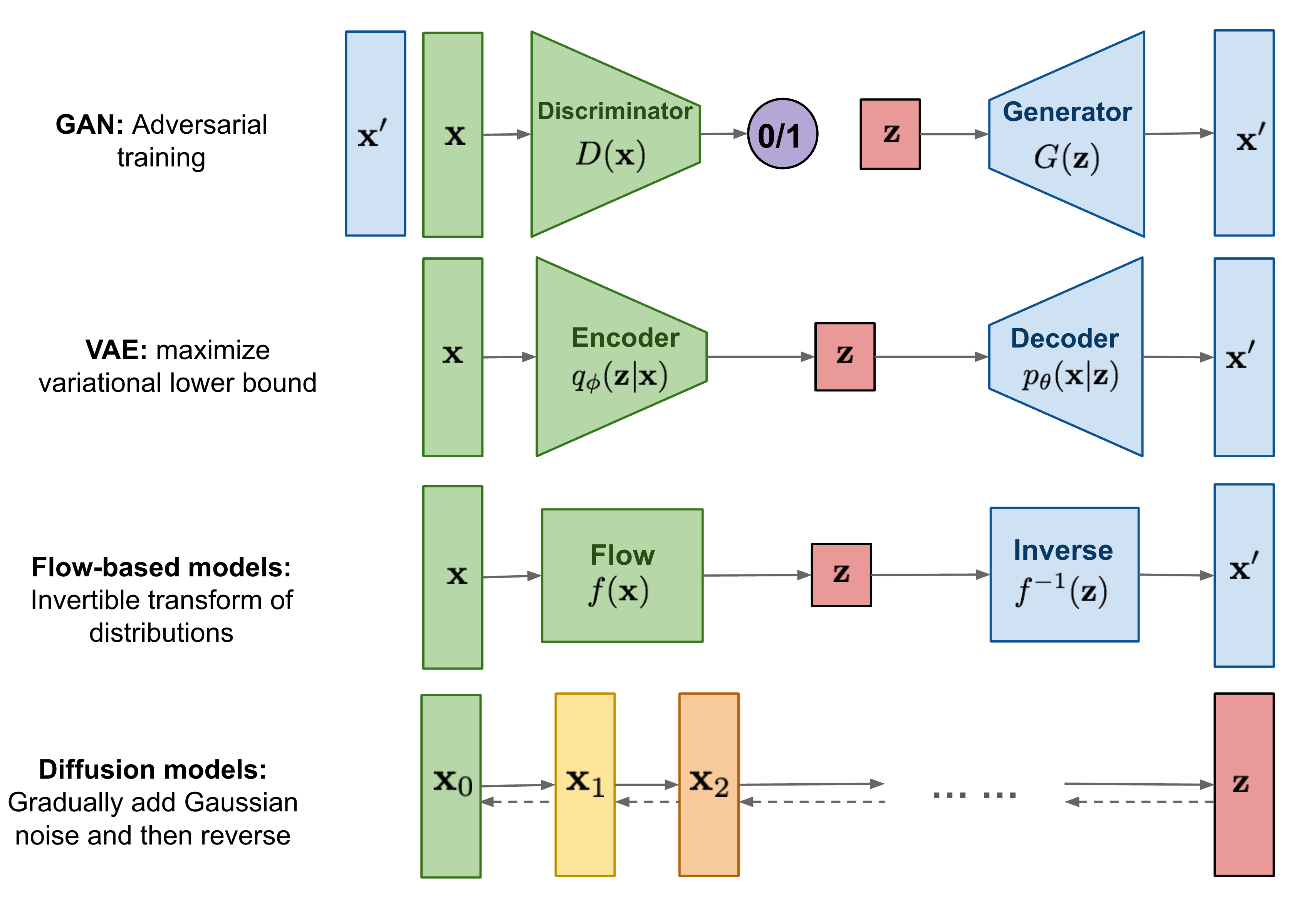
Generative modeling is a central problem in machine learning, concerned with learning a probability distribution \(p(x)\) from which new, realistic data samples can be drawn. Over the past decade, three families of generative models have dominated the literature: Generative Adversarial Networks (GANs), Variational Autoencoders (VAEs), and normalizing flow–based models. Each of these paradigms offers distinct advantages while also exhibiting fundamental limitations.
-
GANs, introduced in Generative Adversarial Nets by Goodfellow et al. (2014), rely on an adversarial training framework in which a generator and discriminator compete in a minimax game. While GANs are capable of producing highly sharp and realistic samples, their training dynamics are notoriously unstable and sensitive to hyperparameters, often suffering from mode collapse and lack of diversity (cf. On the Convergence and Stability of GANs by Mescheder et al. (2018)). Moreover, GANs do not provide an explicit likelihood, i.e., they do not assign a clear probability to how likely a given data sample is under the model. This makes it difficult to objectively compare different models or measure how well a model has learned the data distribution. As a result, GANs are less suitable for applications that require reliable uncertainty estimates, principled evaluation metrics, or probabilistic decision-making.
-
VAEs, introduced in Auto-Encoding Variational Bayes by Kingma and Welling (2013), take a probabilistic approach by optimizing a variational lower bound on the data likelihood. VAEs are stable to train and provide an explicit generative density, but the reliance on surrogate objectives—such as Gaussian likelihood assumptions and KL regularization—often leads to overly smooth or blurry samples, particularly in image generation tasks.
-
Flow-based models, such as those introduced in Density Estimation using Real NVP by Dinh et al. (2016) and Glow: Generative Flow with Invertible 1×1 Convolutions by Kingma and Dhariwal (2018), address likelihood estimation directly via exact change-of-variables formulas. However, they require carefully designed invertible architectures with tractable Jacobians, which significantly constrains model design and increases implementation complexity.
Emergence of Diffusion Models
-
Diffusion models present a compelling alternative to these earlier generative paradigms. Inspired by ideas from non-equilibrium thermodynamics, diffusion models define a stochastic process that incrementally transforms data into noise through a fixed forward process, and then learn to reverse (i.e., invert) this process by denoising it step-by-step in order to generate samples. Unlike GANs, diffusion models do not rely on adversarial training, and unlike VAEs and flow-based models, they do not require restrictive architectural constraints or surrogate likelihood assumptions.
-
The foundational idea of diffusion-based generative modeling was introduced in Deep Unsupervised Learning using Nonequilibrium Thermodynamics by Sohl-Dickstein et al. (2015). In this work, the authors proposed modeling data generation as the reversal of a gradual diffusion process, framing learning as approximating the reverse-time dynamics of a Markov chain that incrementally adds Gaussian noise.
-
Subsequent breakthroughs significantly improved the scalability and practicality of diffusion models. In Generative Modeling by Estimating Gradients of the Data Distribution by Song and Ermon (2019), the authors introduced score-based generative modeling, showing that learning the gradient of the log-density of noisy data distributions suffices for generation. Shortly thereafter, Denoising Diffusion Probabilistic Models by Ho et al. (2020) reformulated diffusion models using a simplified and highly stable training objective based on noise prediction, dramatically improving sample quality and ease of implementation.
-
A concise visual overview situating diffusion models among other generative approaches is provided in the diagram below from Lilian Weng’s blog post “What are Diffusion Models?”:
Practical Adoption
-
Diffusion models are conceptually simple yet remarkably powerful. Their training procedure is stable, does not require adversarial objectives, and scales effectively with model size and data. As a result, diffusion models have rapidly become the dominant paradigm for high-fidelity generative modeling across multiple modalities, including images, audio, and video.
-
They form the core of several landmark systems for conditional and unconditional generation. Notable examples include GLIDE proposed in GLIDE: Towards Photorealistic Image Generation and Editing with Text-Guided Diffusion Models by Nichol et al. (2021), DALL·E 2 proposed in Hierarchical Text-Conditional Image Generation with CLIP Latents by Ramesh et al. (2022), Latent Diffusion Models proposed in High-Resolution Image Synthesis with Latent Diffusion Models by Rombach et al. (2022), Imagen proposed in Photorealistic Text-to-Image Diffusion Models with Deep Language Understanding by Saharia et al. (2022), and Stable Diffusion, developed by Stability AI.
-
These systems demonstrate that diffusion models are capable of matching or surpassing prior state-of-the-art generative approaches in both sample quality and controllability, while maintaining a principled probabilistic foundation.
-
Diffusion models are a relatively recent paradigm and remain an active area of research. Ongoing work explores faster and more efficient sampling methods, improved conditioning mechanisms, continuous-time formulations, and stronger theoretical guarantees. At the same time, core design choices such as optimal noise schedules, sampling algorithms, and architectural inductive biases are still being actively investigated. Their rapid adoption across academic research and industrial-scale systems highlights their growing importance as a unifying framework for modern generative modeling.
Overview
-
The rapid ascent of diffusion models represents one of the most significant developments in generative modeling over the past several years. Beginning as a theoretically motivated alternative to adversarial and variational approaches, diffusion models have evolved into a highly practical and dominant paradigm for high-fidelity data generation across a wide range of modalities.
-
Diffusion models are a class of likelihood-based generative models that construct complex data distributions through a sequence of simple stochastic transformations. Rather than generating samples in a single step, diffusion models define a multi-step process in which data are gradually corrupted by noise and then reconstructed by reversing this corruption. This incremental formulation enables diffusion models to decompose a challenging global modeling problem into a series of tractable local denoising tasks.
-
A sequence of influential papers in the early 2020s demonstrated that diffusion models can not only rival but often outperform GANs in terms of sample quality, training stability, and coverage of the data distribution; in particular, Diffusion Models Beat GANs on Image Synthesis by Dhariwal and Nichol (2021) reported Fréchet Inception Distance (FID) scores of 2.97 on ImageNet 128×128, 4.59 on ImageNet 256×256, and 7.72 on ImageNet 512×512, and showed that with classifier guidance diffusion models achieve FID as low as 3.94 at 256×256 and 3.85 at 512×512, matching or surpassing state-of-the-art GAN performance (specifically BigGAN-deep) while remaining more stable to train.
-
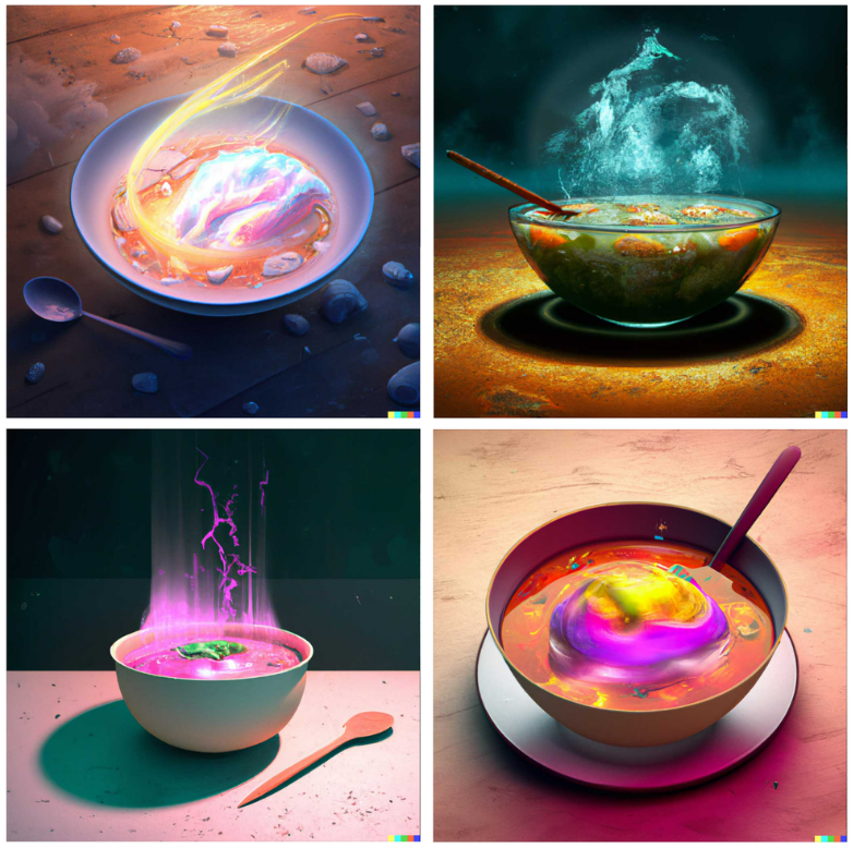
More recently, diffusion models have formed the backbone of several widely publicized generative systems. A notable example is DALL·E 2, introduced in Hierarchical Text-Conditional Image Generation with CLIP Latents by Ramesh et al. (2022), which uses diffusion in a learned latent space to generate photorealistic images conditioned on natural language prompts. A high-level explanation of this system can be found in the blog post: How DALL·E 2 Actually Works by AssemblyAI. The following figure shows example images generated by a diffusion-based text-to-image model, illustrating how diverse, coherent visual concepts can be synthesized from natural language descriptions.
-
The success of these systems has sparked widespread interest among machine learning practitioners and researchers alike. Diffusion models are now routinely applied to problems in image synthesis, audio generation, video modeling, super-resolution, inpainting, and multimodal generation, often serving as the core generative component in large, modular pipelines.
-
From a conceptual standpoint, diffusion models are appealing because they combine several desirable properties:
- they are trained using simple regression-style objectives rather than adversarial losses,
- they admit clear probabilistic interpretations,
- and they scale reliably with model capacity and dataset size.
-
At the same time, diffusion models are flexible enough to incorporate a wide range of architectural choices, conditioning mechanisms, and sampling strategies. Modern implementations commonly integrate convolutional neural networks, attention mechanisms, transformers, and learned latent representations, while still adhering to the same underlying diffusion framework.
-
In this primer, we aim to demystify diffusion models by examining both their theoretical foundations and their practical implementation details. We begin by introducing the core principles that govern diffusion-based generative modeling, followed by a detailed exploration of the mathematical structure underlying diffusion processes. Building on this foundation, we then examine how diffusion models are instantiated in practice, including architectural design choices, training objectives, and sampling algorithms. Finally, we demonstrate how diffusion models can be implemented in PyTorch to generate images, providing concrete intuition for how these models operate end-to-end.
Introduction
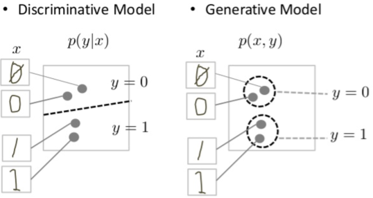
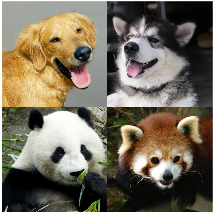
- Diffusion probabilistic models—commonly referred to as diffusion models—are a class of generative models designed to learn complex data distributions and generate new samples that resemble the training data. As generative models, their purpose is fundamentally different from that of discriminative models: rather than predicting labels or making decisions based on inputs, diffusion models aim to synthesize new data that are statistically similar to observed examples. For instance, a diffusion model trained on a dataset of animal images can generate novel images that appear to depict realistic animals, whereas a discriminative model would be tasked with classifying an image as containing a cat or a dog.
- The following figure shows a conceptual comparison between discriminative and generative modeling paradigms, highlighting how discriminative models learn decision boundaries for predicting labels, while generative models learn the joint data distribution in order to synthesize new samples.
-
At a high level, diffusion models operate by defining two complementary stochastic processes:
- A fixed forward diffusion process, which progressively corrupts data by adding Gaussian noise, and
- A learned reverse denoising process, which is parameterized by a neural network and gradually removes noise in order to reconstruct data samples.
-
This formulation casts generative modeling as the problem of learning to invert a simple, fixed noising process. Starting from pure noise, the learned reverse process iteratively transforms noise into structured data. This perspective was formalized in Deep Unsupervised Learning using Nonequilibrium Thermodynamics by Sohl-Dickstein et al. (2015) and later refined and popularized through more practical formulations.
-
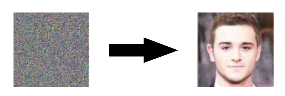
Conceptually, diffusion models can be understood as parameterized Markov chains trained to denoise data one step at a time. After training, generation proceeds by sampling an initial noise vector—often referred to as a latent tensor—and repeatedly applying the learned denoising transitions until a data sample is obtained. In this sense, diffusion models transform an unstructured collection of random numbers into a coherent output, such as an image, through a long sequence of small, incremental refinements.
-
Diffusion models are also closely related to several existing ideas in the generative modeling literature. They can be viewed as a form of latent variable model, in which the latent variables \(x_1, \ldots, x_T\) have the same dimensionality as the observed data \(x_0\). They share conceptual similarities with denoising autoencoders, which learn to reconstruct clean data from corrupted inputs, as discussed in A Connection Between Score Matching and Denoising Autoencoders by Vincent (2011). In addition, diffusion models are tightly connected to score-based generative modeling, where the goal is to estimate gradients of log-density functions rather than explicit likelihoods (cf. Generative Modeling by Estimating Gradients of the Data Distribution by Song and Ermon (2019)).
-
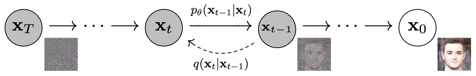
The overall generation process is illustrated in the diagram below (source). The model begins from random noise and progressively refines the sample through repeated denoising steps.
-
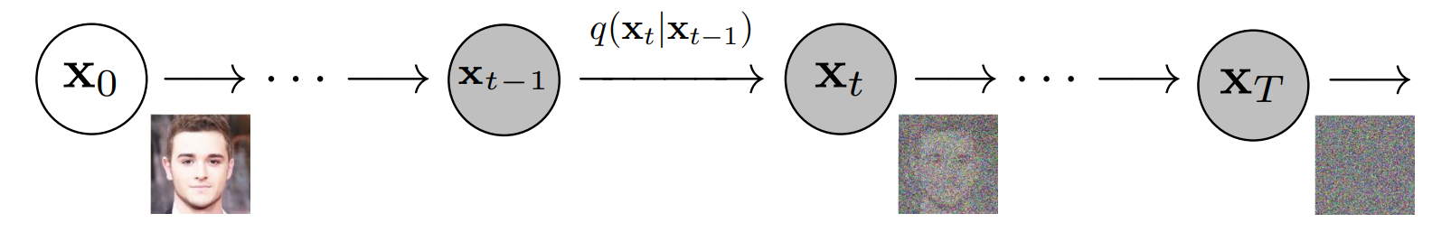
More formally, diffusion models define a latent-variable formulation in which a fixed Markov chain maps a data sample \(x_0\) to a sequence of progressively noisier variables \(x_1, \ldots, x_T\). The joint distribution of these variables under the forward process is denoted as:
\[q(x_{1:T} \mid x_0)\]- where each \(x_t\) has the same dimensionality as the original data. In the context of image generation, this corresponds to repeatedly adding small amounts of Gaussian noise to an image until the final variable \(x_T\) is approximately indistinguishable from isotropic Gaussian noise, meaning noise whose statistical properties are identical in all directions and dimensions.
-
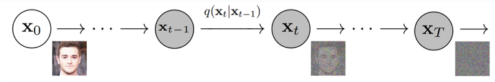
This forward diffusion process is visualized below (source), with each step incrementally destroying structure in the data:

-
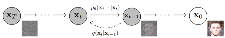
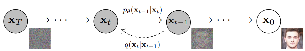
The objective of training a diffusion model is to learn the reverse process, denoted as:
\[p_\theta(x_{t-1} \mid x_t)\]- which approximates the inverse of each forward noising step. By traversing this learned reverse chain from \(t = T\) down to \(t = 0\), the model can transform pure noise into a structured data sample. This reverse-time generation process is illustrated below (source):

-
Under the hood, diffusion models rely on the Markov property, meaning that each state in the diffusion chain depends only on the immediately preceding (or following) state. A Markov chain is a stochastic process in which future states are conditionally independent of past states given the present state. This property allows diffusion models to decompose generation into a sequence of local transitions, each of which is relatively simple to model.
-
Key takeaway: diffusion models are constructed by first specifying a simple and tractable procedure for gradually turning data into noise, and then training a neural network to invert this procedure step-by-step. Each denoising step removes a small amount of noise and restores a small amount of structure. When this process is repeated sufficiently many times—starting from pure noise—the result is a coherent data sample. This deceptively simple idea underlies the remarkable effectiveness of diffusion models in modern generative modeling.
Transformers vs. Diffusion Models
- Transformers and diffusion models are two complementary families of generative models that differ primarily in (i) what conditional distribution they learn during training and (ii) how they generate samples at inference time, with modern systems increasingly mixing the two by using Transformer backbones inside diffusion pipelines (for example, Diffusion Transformer (DiT) in Scalable Diffusion Models with Transformers by Peebles and Xie (2022)).
- A detailed overview of the Transformer architecture has been offered in our Transformers primer.
High-level comparison
-
What is modeled:
- Transformers typically model a factorized (often autoregressive) likelihood over tokens, using self-attention as introduced in Attention Is All You Need by Vaswani et al. (2017).
- Diffusion models typically define a simple prior and learn a denoising reverse process that transforms noise into data, as in Denoising Diffusion Probabilistic Models by Ho et al. (2020).
-
How samples are generated:
- Autoregressive Transformers sample sequentially, token-by-token, following the learned conditional factors (as scaled in large language models such as Language Models are Few-Shot Learners by Brown et al. (2020)).
- Diffusion models sample by starting from Gaussian noise and iteratively denoising over a sequence of timesteps (or continuous time), as in Denoising Diffusion Probabilistic Models by Ho et al. (2020) and the continuous-time unification in Score-Based Generative Modeling through Stochastic Differential Equations by Song et al. (2020).
Training objectives
-
Transformers: maximum-likelihood via token prediction:
-
A standard autoregressive objective is negative log-likelihood:
\[L_{\text{AR}}(\theta) =-\mathbb{E}_{x} \left[ \sum_{i=1}^{n} \log p_\theta(x_i \mid x_{<i}) \right]\]- which underpins large-scale decoder-only Transformers (for example, Language Models are Few-Shot Learners by Brown et al. (2020)).
-
A common non-autoregressive alternative is masked language modeling:
\[L_{\text{MLM}}(\theta) =-\mathbb{E}_{x,m} \left[ \sum_{i\in m} \log p_\theta(x_i \mid x_{\setminus m}) \right]\]- as in BERT: Pre-training of Deep Bidirectional Transformers for Language Understanding by Devlin et al. (2018).
-
-
Diffusion: denoising / noise prediction:
-
A canonical DDPM training objective learns to predict the injected Gaussian noise:
\[L_{\text{DDPM}}(\theta) =\mathbb{E}_{x_0,t,\epsilon} \left[ \left\lVert \epsilon - \epsilon_\theta(x_t,t) \right\rVert^2 \right]\]- where \(x_t\) is a noised version of \(x_0\) and \(\epsilon \sim \mathcal{N}(0,I)\), as in Denoising Diffusion Probabilistic Models by Ho et al. (2020).
-
In continuous-time score-based diffusion, the learned object is the score field that drives reverse-time dynamics, unifying diffusion and score matching in Score-Based Generative Modeling through Stochastic Differential Equations by Song et al. (2020).
-
Sampling and computational trade-offs
-
Transformers:
- Sampling is typically sequential across tokens, which can be a bottleneck for long sequences even though each step is a single forward pass (as in Language Models are Few-Shot Learners by Brown et al. (2020)).
- For images, Transformers often require a tokenization scheme (e.g., patches or discrete codes) and then generate tokens sequentially; Transformers are widely used for vision representations via patch tokenization as in An Image is Worth 16x16 Words: Transformers for Image Recognition at Scale by Dosovitskiy et al. (2020).
-
Diffusion models:
- Sampling is iterative across diffusion timesteps: starting from \(x_T \sim \mathcal{N}(0,I)\) and applying repeated denoising updates, as in Denoising Diffusion Probabilistic Models by Ho et al. (2020).
- Accelerated samplers reduce the number of required steps by changing the sampling trajectory without changing training, as in Denoising Diffusion Implicit Models by Song et al. (2020), and continuous-time solvers offer SDE/ODE-based alternatives in Score-Based Generative Modeling through Stochastic Differential Equations by Song et al. (2020).
Data modality fit
-
Transformers:
- Natural fit for discrete sequences (text, code), using attention for long-range dependencies as introduced in Attention Is All You Need by Vaswani et al. (2017).
- Strong for representation learning in vision via patch tokens, as in An Image is Worth 16x16 Words: Transformers for Image Recognition at Scale by Dosovitskiy et al. (2020).
-
Diffusion models:
- Particularly strong for high-fidelity generation of continuous signals (images, audio, video), with likelihood-based, stable training in Denoising Diffusion Probabilistic Models by Ho et al. (2020).
- Efficient large-scale image systems often run diffusion in a learned latent space for speed, as in High-Resolution Image Synthesis with Latent Diffusion Models by Rombach et al. (2022).
Convergence: Transformer backbones inside diffusion
- A key modern trend is that “Transformer vs. diffusion” is often not an either-or choice: diffusion defines the generative process, while Transformers can serve as the denoiser backbone.
- DiT replaces the U-Net denoiser with a Transformer operating on latent patches and shows favorable scaling behavior, as in Scalable Diffusion Models with Transformers by Peebles and Xie (2022).
- In this setup, diffusion training still uses a denoising objective (e.g., noise prediction), but \(\epsilon_\theta(\cdot)\) is parameterized by a Transformer rather than a convolutional U-Net, as described in Scalable Diffusion Models with Transformers by Peebles and Xie (2022).
Advantages
- Diffusion models offer a combination of theoretical elegance, empirical performance, and practical robustness that has driven their rapid adoption across modern generative modeling applications. Their advantages span sample quality, training stability, scalability, and flexibility, positioning them as a compelling alternative to earlier generative paradigms such as GANs, VAEs, and flow-based models.
High-Fidelity Sample Quality
-
One of the most striking advantages of diffusion models is their ability to produce state-of-the-art sample quality, particularly in high-resolution image generation. Empirical evaluations have shown that diffusion models consistently achieve lower Fréchet Inception Distance (FID) scores than competing GAN-based approaches on standard benchmarks.
-
This result was demonstrated explicitly in Diffusion Models Beat GANs on Image Synthesis by Dhariwal and Nichol (2021), where diffusion models surpassed BigGAN-style architectures in both image fidelity and diversity. The figure below (source) illustrates the qualitative improvements achieved by diffusion-based generators:
- Unlike GANs, which often trade off diversity for sharpness due to adversarial dynamics, diffusion models naturally balance these objectives by modeling the full data distribution through a likelihood-based framework.
Stable and Non-Adversarial Training
-
Diffusion models avoid the instability inherent to adversarial training. GANs require carefully balanced updates between a generator and discriminator, and even minor imbalances can lead to divergence or mode collapse (cf. On the Convergence and Stability of GANs by Mescheder et al. (2018)). In contrast, diffusion models are trained using simple regression-style objectives, most commonly mean squared error losses that predict injected Gaussian noise.
-
This non-adversarial setup results in:
- predictable optimization behavior,
- reduced sensitivity to hyperparameters,
- and reliable convergence across a wide range of datasets and model scales.
-
As shown in Denoising Diffusion Probabilistic Models by Ho et al. (2020), diffusion training objectives can be derived directly from variational likelihood bounds, providing both empirical stability and probabilistic justification.
Explicit Probabilistic Interpretation
-
Diffusion models admit a clear probabilistic interpretation grounded in latent-variable modeling and Markov chains. The forward diffusion process is fixed and analytically tractable, while the reverse process is learned to approximate the true reverse-time dynamics.
-
This structure enables:
- principled likelihood estimation (or lower bounds thereof),
- theoretical analysis using tools from stochastic processes,
- and direct connections to score matching and Stochastic Differential Equations (SDEs).
-
In particular, the unification of diffusion models with continuous-time stochastic processes in Score-Based Generative Modeling through Stochastic Differential Equations by Song et al. (2021) provides a rigorous mathematical framework that explains why diffusion-based approaches are effective and how different sampling methods relate to one another.
Scalability and Parallelization
-
Diffusion models scale exceptionally well with both model capacity and dataset size. Training can be parallelized efficiently across large batches and distributed systems because each training example involves independent noise corruption and denoising prediction.
-
Moreover, architectural choices such as U-Net-based or Transformer-based backbones can be incorporated without altering the core diffusion objective. This scalability has enabled diffusion models to serve as the backbone of large-scale systems such as:
- Imagen (cf. Photorealistic Text-to-Image Diffusion Models with Deep Language Understanding by Saharia et al. (2022)),
- DALL·E 2 (cf. Hierarchical Text-Conditional Image Generation with CLIP Latents by Ramesh et al. (2022)),
- and Stable Diffusion developed by Stability AI.
Flexibility Across Modalities and Conditioning Schemes
-
Diffusion models are highly adaptable and have been successfully applied to a wide range of data modalities, including images, audio, video, 3D data, and multimodal settings. Conditioning mechanisms—such as class labels, text embeddings, semantic maps, or other structured inputs—can be integrated naturally via concatenation, cross-attention, or feature-wise modulation.
-
This flexibility is exemplified by models such as GLIDE proposed in GLIDE: Towards Photorealistic Image Generation and Editing with Text-Guided Diffusion Models by Nichol et al. (2021), and Latent Diffusion Models proposed in High-Resolution Image Synthesis with Latent Diffusion Models by Rombach et al. (2022).
-
Because the diffusion objective remains unchanged, these conditioning strategies can be added without destabilizing training.
Definitions
- This section introduces the core concepts and components that recur throughout diffusion-based generative modeling. These definitions establish a shared vocabulary for understanding diffusion models at both a theoretical and practical level.
Diffusion Models
-
Diffusion models are neural generative models that learn to approximate the reverse of a stochastic diffusion process. Concretely, a diffusion model parameterizes conditional distributions of the form:
\[p_\theta(x_{t-1} \mid x_t)\]- where \(x_t\) denotes a noisy version of the data at diffusion timestep \(t\), and \(\theta\) denotes the learnable parameters of the model. The objective is to iteratively transform noisy inputs into cleaner ones until a final sample \(x_0\) is obtained.
-
Diffusion models are typically trained end-to-end to denoise corrupted inputs and produce continuous outputs such as images, audio waveforms, or video frames. Unlike GANs, diffusion models do not rely on adversarial objectives, and unlike flow-based models, they do not require invertible architectures.
-
From an architectural perspective, diffusion models can employ any neural network whose input and output dimensionalities match. In practice, U-Net–style architectures, originally proposed in U-Net: Convolutional Networks for Biomedical Image Segmentation by Ronneberger et al. (2015), dominate due to their ability to preserve spatial structure while integrating global context via skip connections and attention mechanisms. Variants include conditional U-Nets, 3D U-Nets for video or volumetric data, and transformer-based U-Nets for large-scale multimodal generation.
Forward and Reverse Processes
-
Diffusion models consist of two coupled stochastic processes:
- a forward (diffusion) process, which progressively adds noise to data, and
- a reverse (denoising) process, which is learned by the model.
-
The forward process is fixed and typically defined as a Markov chain with Gaussian transitions. The reverse process is parameterized by a neural network and trained to approximate the true reverse-time dynamics. This formulation was introduced in Deep Unsupervised Learning using Nonequilibrium Thermodynamics by Sohl-Dickstein et al. (2015) and refined in later works such as Denoising Diffusion Probabilistic Models by Ho et al. (2020).
Schedulers
-
Schedulers define how noise is added and removed over time during both training and inference. Formally, a scheduler specifies:
- the noise variance schedule \({\beta_t}_{t=1}^T\) or its continuous-time analogue,
- how to compute intermediate quantities such as \(\alpha_t = 1 - \beta_t\) and \(\bar{\alpha}_t = \prod_{s=1}^t \alpha_s\),
- and how to map model predictions to the previous timestep during sampling.
-
Schedulers are algorithmic components rather than neural networks, and they play a critical role in controlling sample quality, stability, and efficiency.
-
Prominent schedulers and samplers include:
- DDPM: introduced in Denoising Diffusion Probabilistic Models by Ho et al. (2020),
- DDIM: introduced in Denoising Diffusion Implicit Models by Song et al. (2020),
- PNDM: proposed in Pseudo Numerical Methods for Diffusion Models on Manifolds by Liu et al. (2022),
- DEIS: introduced in Fast Sampling of Diffusion Models with Discrete Exponential Integrators by Zhang and Chen (2022).
-
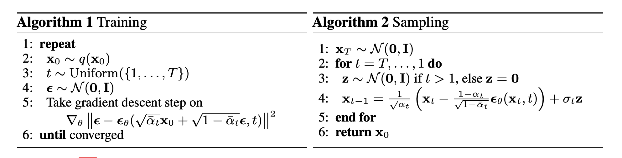
The figure below, adapted from Denoising Diffusion Probabilistic Models by Ho et al. (2020), illustrates the interaction between training and sampling algorithms governed by the scheduler:
Training and Sampling Pipelines
-
In practical systems, diffusion models are rarely deployed in isolation. Instead, they are embedded within end-to-end diffusion pipelines that combine multiple components, such as:
- diffusion models operating at different resolutions,
- text or class encoders for conditional generation,
- super-resolution or refinement models,
- and post-processing stages.
-
These pipelines orchestrate training and inference across multiple models and noise schedules to achieve high-quality generation at scale.
-
Well-known examples include:
- GLIDE GLIDE: Towards Photorealistic Image Generation and Editing with Text-Guided Diffusion Models by Nichol et al. (2021),
- Latent Diffusion Models High-Resolution Image Synthesis with Latent Diffusion Models by Rombach et al. (2022),
- Imagen Photorealistic Text-to-Image Diffusion Models with Deep Language Understanding by Saharia et al. (2022),
- DALL·E 2 Hierarchical Text-Conditional Image Generation with CLIP Latents by Ramesh et al. (2022).
-
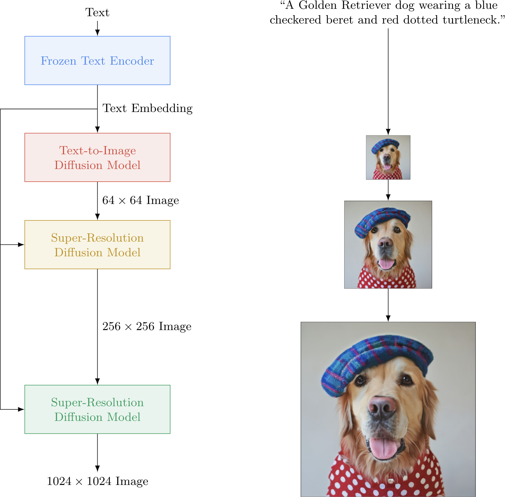
A high-level overview of such a pipeline is shown below (figure adapted from Imagen):
Takeaways
- Diffusion models learn to reverse a fixed noising process via neural denoising.
- Schedulers control the temporal dynamics of noise injection and removal.
-
Sampling pipelines integrate diffusion models with encoders, decoders, and conditioning mechanisms to enable large-scale generation.
- These definitions provide the conceptual building blocks required to understand the mathematical theory of diffusion models, which we examine next.
Diffusion Models: The Theory
- This section develops the theoretical foundations of diffusion models at a conceptual level. Rather than reproducing detailed derivations, we focus on how diffusion models are structured, why they are mathematically well-founded, and how their design choices connect probabilistic modeling, stochastic processes, and modern neural networks. Formal derivations and exact equations are deferred to The Math Under-the-Hood section.
Diffusion Models as Latent-Variable Generative Models
-
Diffusion models belong to the class of latent-variable generative models, meaning that observed data are assumed to arise from a sequence of unobserved random variables. Unlike traditional latent-variable models such as Variational Autoencoders (VAEs), diffusion models introduce a high-dimensional latent trajectory in which every latent variable has the same dimensionality as the observed data.
-
The theoretical motivation for this construction was first introduced in Deep Unsupervised Learning using Nonequilibrium Thermodynamics by Sohl-Dickstein et al. (2015), which framed generation as the reversal of a gradual entropy-increasing process. This idea was later made computationally practical and scalable in Denoising Diffusion Probabilistic Models by Ho et al. (2020).
-
At a high level, diffusion models define:
- A forward process that gradually destroys information in the data by injecting noise.
- A reverse process that learns to recover data by removing noise step by step.
-
This framing transforms generation into a sequence of local denoising problems, each of which is significantly easier than modeling the full data distribution in a single step.
Markovian Structure and Tractability
-
A defining theoretical assumption of diffusion models is the Markov property: each latent variable depends only on its immediate predecessor (in the forward process) or successor (in the reverse process). This choice has several important consequences:
- It enables a clean factorization of joint probability distributions.
- It allows likelihood-based training using variational inference.
- It ensures that learning and sampling can be performed with bounded memory and computation per timestep.
-
The Markov structure is not merely a modeling convenience; it is essential for making diffusion models analytically tractable and numerically stable. By restricting dependencies to adjacent timesteps, diffusion models avoid the intractable posterior dependencies that often plague deep latent-variable models.
Fixed Forward Process and Learned Reverse Process
-
From a theoretical perspective, one of the most elegant aspects of diffusion models is the asymmetry between the forward and reverse processes:
- The forward diffusion process is fixed and known, chosen by the model designer.
- The reverse diffusion process is unknown and learned, parameterized by a neural network.
-
This asymmetry is crucial. Because the forward process is analytically defined, it induces a known family of corrupted data distributions. The learning problem then reduces to approximating how these corrupted distributions should be inverted.
-
This idea was central to the reformulation of diffusion models in Denoising Diffusion Probabilistic Models by Ho et al. (2020), which showed that learning the reverse process can be cast as a series of regression problems with known targets.
Likelihood-Based Training via Variational Inference
-
Diffusion models are explicit likelihood models. Unlike GANs, which rely on implicit distributions and adversarial training, diffusion models optimize a well-defined objective derived from probability theory.
-
Training proceeds by maximizing a variational lower bound (ELBO) on the data log-likelihood. Conceptually, this objective measures how well the learned reverse process approximates the true reverse of the forward diffusion.
-
The theoretical importance of this formulation is threefold:
- It provides a principled objective grounded in statistical inference.
- It ensures that diffusion models are comparable using likelihood-based metrics.
- It allows training to decompose into a sum of independent per-timestep terms.
-
The use of Gaussian distributions in both forward and reverse processes ensures that all divergence terms appearing in the ELBO are analytically tractable, avoiding the need for high-variance Monte Carlo estimators.
Noise Prediction Parameterization
-
A key theoretical and practical insight introduced in Denoising Diffusion Probabilistic Models by Ho et al. (2020) is that the reverse process need not be parameterized directly in terms of probability distributions.
-
Instead, the model can be trained to predict the noise component that was added during the forward process. This reparameterization has deep theoretical implications:
- It implicitly trains the model to estimate the score function of noisy data distributions.
- It connects diffusion models to denoising score matching, originally developed in Generative Modeling by Estimating Gradients of the Data Distribution by Song and Ermon (2019).
- It yields a simple mean-squared-error objective that is stable across noise levels.
-
This perspective reveals that diffusion models and score-based generative models are not separate paradigms, but rather different parameterizations of the same underlying probabilistic structure.
Connection to Continuous-Time/Score-Based Models
-
Although this section focuses on discrete-time diffusion models, the theory naturally extends to continuous-time formulations. In particular:
- Discrete-time diffusion models can be viewed as numerical discretizations of continuous stochastic processes.
- Learning to predict noise is equivalent to learning the score of a time-dependent distribution.
- Sampling procedures correspond to solving stochastic or deterministic differential equations.
-
These connections were formalized in Score-Based Generative Modeling through Stochastic Differential Equations by Song et al. (2021), which unified DDPMs, DDIMs, and score-based models under a single SDE-based framework.
Discrete Data and Final Decoding
-
A final theoretical consideration concerns the generation of discrete-valued data, such as pixel intensities. While diffusion operates in continuous space, the final output must correspond to discrete observations.
-
Diffusion models address this by defining an explicit likelihood for the final denoising step, typically using discretized continuous distributions. This ensures that diffusion models remain fully probabilistic and that likelihood evaluation is well-defined even for discrete domains.
Takeaways
-
At a theoretical level, diffusion models are characterized by:
- A fixed, analytically tractable forward corruption process.
- A learned reverse denoising process with local dependencies.
- A likelihood-based variational training objective.
- A noise-prediction parameterization linked to score matching.
- A natural extension to continuous-time stochastic processes.
-
These properties collectively explain why diffusion models combine strong theoretical guarantees with exceptional empirical robustness, providing a solid foundation for the architectural and algorithmic design choices explored in subsequent sections.
Diffusion Models: A Deep Dive
- This section connects the theoretical formulation of diffusion models to their concrete operational behavior. We unpack how the forward and reverse processes interact during training and sampling, providing intuition for why diffusion models are effective and how their components work together in practice.
Overview
-
Diffusion models are a form of latent variable model, in which observed data are associated with a sequence of latent states that progressively increase in noise. Latent variable models aim to describe complex data distributions by introducing hidden variables that capture underlying structure in a continuous space, as discussed in Latent Variable Models by The AI Summer.
-
In diffusion models, however, the latent variables \(x_1, \ldots, x_T\) are not lower-dimensional abstractions of the data. Instead, they share the same dimensionality as the observed variable \(x_0\) and represent progressively noisier versions of it. The latent space in diffusion models therefore corresponds to different noise levels rather than semantic compression.
-
Diffusion models consist of two tightly coupled processes:
- A forward diffusion process \(q\) that gradually adds noise to data.
- A reverse denoising process \(p_\theta\) that learns to remove this noise step-by-step.
-
The forward process is fixed by design, while the reverse process is parameterized by a neural network and learned from data.
Forward Diffusion Process
-
The forward process defines a Markov chain that incrementally corrupts a clean data sample \(x_0\). At each timestep \(t\), Gaussian noise is added according to a predefined variance schedule \({\beta_t}_{t=1}^T\).
-
Formally, the forward process is defined as:
\[q(x_t \mid x_{t-1}) =N\left( x_t; \sqrt{1 - \beta_t} x_{t-1}, \beta_t I \right)\]- where \(\beta_t\) controls the magnitude of noise added at step \(t\).
-
Repeating this process for sufficiently large \(T\) ensures that the final variable \(x_T\) is approximately distributed as an isotropic Gaussian:
\[q(x_T) \approx N(0, I)\] -
A key practical insight, introduced in Denoising Diffusion Probabilistic Models by Ho et al. (2020), is that the forward process admits a closed-form solution for sampling \(x_t\) directly from \(x_0\):
\[x_t =\sqrt{\bar{\alpha}_t} , x_0 +\sqrt{1 - \bar{\alpha}_t} \epsilon, \quad \epsilon \sim N(0, I)\]- with \(\bar{\alpha}_t = \prod_{s=1}^t (1 - \beta_s)\). This property allows efficient training by randomly sampling timesteps without explicitly simulating the full forward chain.
-
The forward diffusion process is illustrated below (source), where structured data are gradually transformed into noise through a sequence of small Gaussian perturbations:
Reverse Denoising Process
-
The reverse process is the core learned component of a diffusion model. Its purpose is to invert the forward diffusion dynamics by progressively removing noise.
-
Starting from pure noise \(x_T \sim N(0, I)\), the model applies a sequence of learned reverse transitions:
- Each reverse transition is parameterized as a Gaussian distribution:
-
In practice, the variance \(\Sigma_\theta\) is often fixed or chosen from a small set of options, while the mean \(\mu_\theta\) is predicted by a neural network conditioned on both the noisy input \(x_t\) and the timestep \(t\).
-
This reverse process is illustrated below (source), where noise is gradually transformed back into a structured sample:
Training Procedure and Intuition
-
Training a diffusion model involves teaching the neural network how to denoise inputs at all noise levels. The training loop proceeds as follows:
- Sample a clean data point \(x_0 \sim q(x_0)\).
- Sample a timestep \(t\) uniformly from \({1, \ldots, T}\).
- Sample noise \(\epsilon \sim N(0, I)\).
- Construct a noisy input \(x_t\) using the closed-form forward process.
- Train the network to predict the noise \(\epsilon\) from \(x_t\) and \(t\).
-
This procedure is repeated across batches of data using stochastic gradient descent. Importantly, the network learns a local denoising rule at each timestep rather than a global mapping from noise to data.
Noise Prediction and Score Estimation
- Modern diffusion models are almost always trained to predict the injected noise \(\epsilon\) rather than directly predicting the clean data \(x_0\) or the reverse-process mean. The corresponding loss function is:
-
This formulation has several advantages:
- It yields stable gradients across timesteps.
- It avoids scale issues at high noise levels.
- It connects diffusion models to denoising score matching, as shown in Generative Modeling by Estimating Gradients of the Data Distribution by Song and Ermon (2019).
-
Intuitively, predicting noise is equivalent to estimating the direction in which a noisy sample should be moved to increase data likelihood.
Sampling and Generation
- After training, generation proceeds by initializing \(x_T \sim N(0, I)\) and repeatedly applying the learned reverse transitions:
-
Each step removes a small amount of noise and restores structure. After \(T\) steps, the final output \(x_0\) is obtained.
-
While this procedure yields high-quality samples, it is computationally expensive due to the large number of sequential steps. This limitation motivated the development of accelerated samplers such as DDIM Denoising Diffusion Implicit Models by Song et al. (2020) and ODE-based solvers derived from continuous-time diffusion theory.
Practical Insights
-
From a practical standpoint, diffusion models succeed because they:
- decompose generation into many simple denoising steps,
- train a single network to handle all noise levels,
- and leverage a fixed, well-behaved forward corruption process.
-
This design transforms a challenging generative modeling problem into a sequence of tractable regression tasks, explaining both the robustness and the scalability of diffusion-based approaches.
The Math Under-the-Hood
- At the core of diffusion models lies a probabilistic construction based on Markov chains, Gaussian perturbations, and variational inference. A diffusion model defines a structured latent-variable model in which data are progressively corrupted by noise through a fixed forward process, and then reconstructed through a learned reverse process. This formulation was first proposed in Deep Unsupervised Learning using Nonequilibrium Thermodynamics by Sohl-Dickstein et al. (2015) and later refined into a practical and scalable framework in Denoising Diffusion Probabilistic Models by Ho et al. (2020).
Forward Diffusion Process (Noising)
-
The forward diffusion process is a fixed, non-learned stochastic process that gradually destroys structure in the data by adding Gaussian noise. Let \(x_0 \sim q(x_0)\) denote a data sample drawn from the unknown data distribution. The forward process defines a sequence of latent variables \(x_1, \ldots, x_T\) such that each variable is obtained by perturbing the previous one with a small amount of noise.
-
Formally, the forward process is defined as a Markov chain with Gaussian transition kernels:
\[q\left(x_{1:T} \mid x_0\right) := \prod_{t=1}^{T} q\left(x_t \mid x_{t-1}\right) := \prod_{t=1}^{T} N\left( x_t; \sqrt{1-\beta_t}x_{t-1}, \beta_t I \right)\]-
where:
- \(\beta_t \in (0,1)\) is a variance schedule controlling the amount of noise added at timestep \(t\),
- \(I\) is the identity covariance matrix,
- and \(T\) is the total number of diffusion steps.
-
-
The variance schedule \({\beta_t}_{t=1}^T\) is chosen such that noise increases monotonically over time. For sufficiently large \(T\) and a well-behaved schedule, the final latent variable \(x_T\) converges in distribution to an isotropic Gaussian:
-
A crucial property of this construction, derived in Denoising Diffusion Probabilistic Models by Ho et al. (2020), is that the marginal distribution \(q(x_t \mid x_0)\) admits a closed-form expression:
\[x_t =\sqrt{\bar{\alpha}_t}x_0 +\sqrt{1-\bar{\alpha}_t}\epsilon, \quad \epsilon \sim N(0, I),\]-
where:
\[\alpha_t = 1 - \beta_t, \qquad \bar{\alpha}_t = \prod_{s=1}^{t} \alpha_s\]
-
-
This result allows direct sampling of \(x_t\) from \(x_0\) at any timestep \(t\) without explicitly simulating the entire forward chain, which is critical for efficient training.
-
The joint structure of the forward diffusion process is visualized below (figure adapted from Denoising Diffusion Probabilistic Models by Ho et al. (2020)):
Reverse Diffusion Process (Denoising)
-
The generative power of diffusion models arises from learning the reverse diffusion process, which inverts the forward noising dynamics. While the forward process is analytically defined, the true reverse process \(q(x_{t-1} \mid x_t)\) is generally intractable. Diffusion models therefore learn a parametric approximation to this reverse process.
-
The learned generative model defines the joint distribution:
\[p_\theta(x_{0:T}) := p(x_T) \prod_{t=1}^{T} p_\theta(x_{t-1} \mid x_t)\]- where the prior over the final latent variable is fixed as:
-
Each reverse transition is parameterized as a Gaussian:
\[p_\theta(x_{t-1} \mid x_t) =N\left( x_{t-1}; \mu_\theta(x_t, t), \Sigma_\theta(x_t, t) \right)\]-
with:
- \(\mu_\theta(x_t, t)\) denoting the predicted mean,
- \(\Sigma_\theta(x_t, t)\) denoting the predicted or fixed covariance,
- and \(\theta\) representing the parameters of a neural network conditioned on \(x_t\) and the timestep \(t\).
-
-
The Markov property plays a crucial role here: each reverse transition depends only on the current noisy state \(x_t\) and not on earlier or later latent variables. This conditional independence enables tractable likelihood bounds and efficient training.
-
The reverse diffusion chain is illustrated below (figure adapted from Denoising Diffusion Probabilistic Models by Ho et al. (2020)):
Variational Learning Perspective
-
Training diffusion models is framed as variational inference, because the intractable true posterior \(p_\theta(x_{1:T}\mid x_0)\) is replaced by a parameterized, tractable variational distribution \(q(x_{1:T}\mid x_0)\) whose parameters are optimized to tighten a variational (evidence) lower bound, also called the ELBO, on the data log-likelihood:
\[\log p_\theta(x_0) \ge \mathbb{E}_{q(x_{1:T}\mid x_0)} \left[ \log p_\theta(x_{0:T}) -\log q(x_{1:T}\mid x_0) \right] \equiv \mathcal{L}_{\text{VLB}}\]- where:
- \(x_0\) denotes an observed data sample.
- \(x_{1:T}\) denotes the sequence of latent variables (noise states) along the diffusion trajectory.
- \(p_\theta(x_{1:T}\mid x_0)\) is the true (intractable) posterior, representing the distribution over latent diffusion trajectories given data.
- \(q(x_{1:T}\mid x_0)\) is the variational posterior, a tractable approximation to the true posterior constructed from the known forward noising process.
- \(p_\theta(x_{0:T})\) is the joint generative model,
- Factorized as: \(p_\theta(x_{0:T}) = p(x_T)\prod_{t=1}^{T} p_\theta(x_{t-1}\mid x_t)\)
- With prior: \(p(x_T)=\mathcal{N}(0,I)\)
- \(\log p_\theta(x_{0:T})\) measures how well a latent trajectory explains the data under the model.
- \(\log q(x_{1:T}\mid x_0)\) penalizes divergence from the variational posterior.
- \(\mathbb{E}_{q(x_{1:T}\mid x_0)}[\cdot]\) denotes expectation over diffusion trajectories sampled from the variational posterior.
- \(\mathcal{L}_{\text{VLB}}\) is the variational (evidence) lower bound on \(\log p_\theta(x_0)\).
- where:
-
Due to the Markov structure and Gaussian assumptions, the ELBO decomposes into a sum of Kullback–Leibler divergence terms between forward and reverse transition distributions, plus a reconstruction term at the final step:
- Because both the forward and reverse transitions are Gaussian, all KL divergence terms admit closed-form expressions. This tractability distinguishes diffusion models from many other latent-variable models and avoids reliance on high-variance Monte Carlo estimators.
Noise Prediction Parameterization
- A key empirical insight introduced in Denoising Diffusion Probabilistic Models by Ho et al. (2020) is that training becomes significantly simpler and more stable when the model is parameterized to predict the noise \(\epsilon\) rather than the reverse-process mean directly.
- Predicting the reverse-process mean \(\mu_\theta(x_t,t)\) requires the model to explicitly account for the noise schedule and the time-dependent correlations between \(x_t\) and \(x_0\), making the learning target vary in scale and structure across timesteps. In contrast, predicting the noise \(\epsilon\) yields a fixed, well-conditioned target drawn from a simple isotropic Gaussian distribution at all timesteps, meaning the noise has identical variance in every dimension and no preferred direction or correlation structure, i.e., its covariance matrix is proportional to the identity.
- Direct mean prediction appears in early diffusion formulations such as Deep Unsupervised Learning using Nonequilibrium Thermodynamics by Sohl-Dickstein et al. (2015) and as an explicit parameterization option in Denoising Diffusion Probabilistic Models by Ho et al. (2020), but it has been largely superseded in practice by noise prediction in modern U-Net–based diffusion models (e.g., DDPMs and LDMs) and Transformer-based diffusion architectures (e.g., DiTs), due to improved stability and empirical performance.
- Under this parameterization, the neural network \(\epsilon_\theta(x_t, t)\) is trained to approximate the noise used to generate \(x_t\):
-
This yields the widely used simplified training objective:
\[L_{\text{simple}}(\theta) =\mathbb{E}_{x_0, t, \epsilon} \left[ \left\lVert \epsilon -\epsilon_\theta(x_t, t) \right\rVert^2 \right]\]- where \(t\) is sampled uniformly from \({1,\ldots,T}\) and \(\epsilon \sim N(0, I)\).
-
This objective can be interpreted as a form of denoising score matching, establishing a direct connection between diffusion models and score-based generative modeling, as shown in Generative Modeling by Estimating Gradients of the Data Distribution by Song and Ermon (2019).
Takeaways
-
In summary, the mathematical foundation of diffusion models rests on:
- a fixed Gaussian forward diffusion process,
- a learned Gaussian reverse process parameterized by neural networks,
- a variational likelihood objective composed of tractable KL divergences,
- and a noise-prediction parameterization that yields stable and efficient training.
-
This combination of probabilistic rigor and practical simplicity explains why diffusion models are both theoretically well-grounded and empirically successful, and it sets the stage for understanding architectural choices and sampling algorithms in subsequent sections.
Taxonomy of Diffusion Models
-
At a high level, diffusion models can be categorized along two largely orthogonal axes:
- Time formulation: discrete-time versus continuous-time diffusion.
- Representation space: pixel space, latent space, or other learned representations.
-
Historically, the modern diffusion literature emerged in two closely related but initially distinct lines of work. An important precursor is Deep Unsupervised Learning using Nonequilibrium Thermodynamics by Sohl-Dickstein et al. (2015), which introduced a discrete-time, pixel-space gradual noising and denoising framework closely resembling modern diffusion models. Building on this idea, Score-Based Generative Models (SGMs) were introduced in continuous time as a noise-conditional score estimation framework in Generative Modeling by Estimating Gradients of the Data Distribution by Song and Ermon (2019). Shortly thereafter, Denoising Diffusion Probabilistic Models (DDPMs) were proposed in a discrete-time variational framework in Denoising Diffusion Probabilistic Models by Ho et al. (2020). These two perspectives were later shown to be mathematically unified under a continuous-time SDE formulation in Score-Based Generative Modeling through Stochastic Differential Equations by Song et al. (2021).
-
In their most common and practically deployed form, diffusion models are discrete-time models, where noise is added and removed over a finite sequence of timesteps (\(t \in {1,\dots,T}\)). Within this class, diffusion is typically implemented either directly in pixel space or in a learned latent space.
-
More precisely, modern diffusion models usually learn a local denoising rule at each noise level, parameterized by a neural network that predicts one of the following equivalent quantities:
-
the injected Gaussian noise (\(\epsilon\)),
-
the original clean sample (\(x_0\)),
-
or the score (\(\nabla_x \log p_t(x)\)) of the noisy data distribution.
-
These parameterizations are mathematically interchangeable under Gaussian noise assumptions and correspond to different but equivalent views of the reverse diffusion dynamics. The equivalence between noise prediction and score matching provides the conceptual bridge between discrete-time DDPMs and continuous-time SGMs.
-
-
Mathematically speaking, in discrete-time diffusion models, the reverse model is typically trained via a denoising objective that matches the model’s prediction (most commonly \(\epsilon_\theta(x_t, t)\)) to the true Gaussian noise used to construct \(x_t\) from \(x_0\). Generation then emerges by repeatedly applying the learned update rule across discrete timesteps, starting from \(t = T\) and proceeding down to \(t = 0\).
- This discrete-time framing has proven remarkably robust, as it allows complex data distributions to be learned via simple Gaussian perturbations and local denoising steps rather than direct density modeling. Canonical examples of this class include Denoising Diffusion Probabilistic Models (DDPMs) introduced in 2020, and their accelerated samplers such as Denoising Diffusion Implicit Models (DDIMs) introduced shortly thereafter in Denoising Diffusion Implicit Models by Song et al. (2020).
-
Continuous-time diffusion models generalize this perspective by describing the forward and reverse processes as SDEs defined over a continuous time variable (\(t \in [0,1]\)). In this formulation, diffusion is no longer tied to a fixed number of discrete noise levels but instead evolves according to continuous stochastic dynamics.
- Importantly, this continuous-time view is representation-agnostic: the same SDE framework applies whether diffusion is performed in pixel space, latent space, or another learned representation. Discrete-time diffusion models such as DDPMs and DDIMs can be recovered as specific numerical discretizations of these continuous-time processes, while earlier SGMs correspond to directly learning the score field required to solve the reverse-time SDE.
-
In practice, most large-scale systems rely on latent-space, discrete-time diffusion models trained with Denoising Diffusion Probabilistic Model (DDPM)–style objectives, especially in image, video, and multimodal generation, due to their favorable trade-off between sample quality and computational cost. This design choice was popularized by Latent Diffusion Models (LDMs) in High-Resolution Image Synthesis with Latent Diffusion Models by Rombach et al. (2022), which introduced diffusion in a learned latent space while retaining discrete-time training.
-
Sampling in modern systems is most commonly performed using DDIM–like deterministic or partially deterministic discrete-time samplers, or probability-flow ODE solvers derived from the continuous-time Stochastic Differential Equation (SDE) framework.
-
By contrast, pure pixel-space discrete-time DDPMs and standalone continuous-time Score-Based Generative Models (SGMs) based on Langevin dynamics are now primarily used for research, benchmarking, or specialized domains where fidelity, theoretical clarity, or likelihood estimation is prioritized over raw sampling speed.
Discrete-Time Diffusion Models
-
Discrete-time diffusion models formulate generative modeling as a finite sequence of noising and denoising steps indexed by a timestep variable \(t \in {1,\dots,T}\). At each step, small amounts of Gaussian noise are added to data, and a neural network is trained to gradually remove this noise to recover clean samples.
-
This perspective originated in Deep Unsupervised Learning using Nonequilibrium Thermodynamics by Sohl-Dickstein et al. (2015) and was popularized in its modern form by Denoising Diffusion Probabilistic Models by Ho et al. (2020).
-
From a taxonomy standpoint, discrete-time diffusion models occupy the time-discretized branch of the diffusion landscape and can be instantiated in different representation spaces:
- Pixel-space discrete-time diffusion models, where diffusion operates directly on raw data.
- Latent-space discrete-time diffusion models, where diffusion operates in a learned compressed representation.
-
Discrete-time diffusion models typically learn a local denoising rule at each noise level, parameterized by a neural network that predicts an equivalent quantity such as injected noise, the original clean sample, or the score of the noisy distribution.
-
Sampling proceeds by starting from pure Gaussian noise and repeatedly applying the learned denoising updates across timesteps. Although this yields high-quality samples, it can require many sequential steps.
-
Faster discrete-time sampling methods, such as Denoising Diffusion Implicit Models (DDIMs) introduced in Denoising Diffusion Implicit Models by Song et al. (2020), follow alternative deterministic or partially stochastic trajectories through the same discrete noise levels without changing training.
-
In modern practice, discrete-time diffusion models form the practical backbone of large-scale image, video, and multimodal generation systems, often combined with latent representations and accelerated samplers.
-
Having introduced discrete-time diffusion models along the time-formulation axis, we now turn to the representation-space axis and first examine pixel-space diffusion models, where the diffusion process operates directly on raw data such as image pixels or audio waveforms.
Pixel-Space Diffusion Models
-
Pixel-space diffusion models operate directly on high-dimensional data representations such as image pixels or raw audio waveforms. In this setting, the diffusion process acts on the original data coordinates, and no intermediate learned representation is introduced. As a result, pixel-space diffusion models offer a clear probabilistic interpretation and can achieve very high sample fidelity.
-
From a hierarchical perspective, pixel-space diffusion models can be further divided according to their time formulation:
- Discrete-time pixel-space diffusion models, where noise is added and removed over a finite sequence of timesteps.
-
Continuous-time pixel-space diffusion models, where diffusion is defined via SDEs and score matching.
- Historically and practically, discrete-time pixel-space diffusion models appeared first and form the conceptual foundation of the field.
-
While pixel-space diffusion enables precise modeling of fine-grained details, it also leads to substantial computational costs. The dimensionality of pixel data is extremely high, and both training and sampling require repeated neural network evaluations over many diffusion steps. These limitations motivated the development of latent-space diffusion models, which apply the same principles in a compressed representation.
-
Despite these costs, pixel-space diffusion models remain important for understanding the theoretical foundations of diffusion-based generative modeling and continue to be used in domains where the highest possible fidelity or exact likelihood computation is required.
Denoising Diffusion Probabilistic Models (DDPMs)
-
Denoising Diffusion Probabilistic Models (DDPMs) are the canonical formulation of discrete-time diffusion-based generative modeling in pixel space. They were introduced in Denoising Diffusion Probabilistic Models by Ho et al. (2020) and define a tractable likelihood-based framework for learning complex data distributions via a sequence of noising and denoising steps indexed by a finite timestep variable.
-
In the hierarchy of diffusion models, DDPMs occupy a central position:
- They are discrete-time rather than continuous-time models.
- They operate directly in pixel space, rather than a learned latent space.
- They explicitly parameterize the reverse diffusion transitions as conditional probability distributions.
-
DDPMs model generation as the reversal of a fixed Markovian diffusion process that gradually destroys structure in the data by injecting Gaussian noise. Learning focuses on approximating the reverse transitions, which ultimately enables sampling from the data distribution starting from pure noise.
-
Overall, DDPMs form the conceptual backbone of modern diffusion models and serve as the starting point for numerous extensions, including accelerated discrete-time samplers (such as DDIMs), continuous-time SDE formulations, and latent-space diffusion models.
-
The Latent: Code the Maths offers a 3-part series covering the mathematical foundations of DDPMs, emphasizing intuition alongside derivations and lightweight code illustrations. Specifically, it offers a concise, math-first walkthrough of the theory behind DDPMs, starting from random variables and distributions, moving through Gaussian and multivariate Gaussian theory, and culminating in the forward/reverse diffusion processes, reparameterization, and training objectives.
Implementation Details
-
Forward (Diffusion / Noising) Process:
- The forward process is a fixed, non-learned Markov chain that progressively adds Gaussian noise to a data sample over \(T\) discrete timesteps. Given an original data point \(x_0\), the transition from timestep \(t-1\) to \(t\) is defined as:
-
where:
- \(q(x_t \mid x_{t-1})\) is the forward diffusion transition distribution from timestep \(t-1\) to \(t\).
- \(x_{t-1}\) is the noisy sample at timestep \(t-1\).
- \(x_t\) is the resulting noisy sample at timestep \(t\).
- \(N(\cdot ; \mu, \Sigma)\) denotes a multivariate Gaussian distribution with mean \(\mu\) and covariance \(\Sigma\).
- \(\beta_t\) is the variance of the Gaussian noise added at timestep \(t\).
- \({\beta_t}_{t=1}^T\) is a predefined variance schedule controlling the amount of noise added at each step.
- \(I\) is the identity covariance matrix.
- \(T\) is the total number of discrete diffusion steps.
-
As \(t\) increases, the signal-to-noise ratio decreases, and for sufficiently large \(T\), the distribution of \(x_T\) approaches a standard Gaussian.
-
A key property of this construction is that the marginal distribution \(q(x_t \mid x_0)\) admits a closed-form expression:
\[x_t = \sqrt{\bar{\alpha}_t} x_0 + \sqrt{1 - \bar{\alpha}_t}\epsilon, \quad \epsilon \sim N(0, I)\]-
where:
- \(q(x_t \mid x_0)\) is the marginal distribution of the noisy sample at timestep \(t\) given the original data.
- \(x_0\) is the original clean data sample.
- \(x_t\) is the noisy version of the data at timestep \(t\).
- \(\epsilon\) is standard Gaussian noise.
- \(\epsilon \sim N(0, I)\) denotes sampling noise from a zero-mean unit-variance Gaussian.
- \(\alpha_t = 1 - \beta_t\) is the noise retention factor at timestep \(t\).
- \(\bar{\alpha}_t = \prod_{s=1}^t \alpha_s\) is the cumulative product of noise retention factors up to timestep \(t\).
-
This closed-form allows training to sample arbitrary timesteps directly without simulating the full forward chain.
-
-
Reverse (Denoising) Process:
-
The reverse process aims to invert the diffusion by learning a parameterized Markov chain that gradually removes noise. Each reverse transition is modeled as a Gaussian distribution:
\[p_\theta(x_{t-1} \mid x_t) = N\left(x_{t-1}; \mu_\theta(x_t, t), \sigma_t^2 I\right)\]-
where:
- \(p_\theta(x_{t-1} \mid x_t)\) is the learned reverse diffusion transition from timestep \(t\) to \(t-1\).
- \(x_t\) is the noisy sample at timestep \(t\).
- \(x_{t-1}\) is the denoised sample at timestep \(t-1\).
- \(N(\cdot;\mu,\Sigma)\) denotes a multivariate Gaussian distribution with mean \(\mu\) and covariance \(\Sigma\).
- \(\mu_\theta(x_t, t)\) is the predicted mean of the reverse transition, produced by a neural network with parameters \(\theta\) and conditioned on the timestep \(t\).
- \(\sigma_t^2\) is the variance of the reverse transition at timestep \(t\).
- \(I\) is the identity covariance matrix.
-
The mean is typically predicted by a U-Net conditioned on \(t\), while \(\sigma_t^2\) may be fixed or learned.
-
-
In practice, DDPMs are commonly parameterized to predict the noise \(\epsilon\) rather than the mean directly. This reparameterization simplifies optimization and improves empirical performance.
-
-
The following figure from the paper illustrates DDPMs as directed graphical models:
-
Training Objective:
- DDPMs are trained by maximizing a variational lower bound on the data log-likelihood. In practice, this objective simplifies to a denoising score-matching loss that minimizes the mean squared error between the true noise and the predicted noise:
-
where:
- \(L\) is the training loss.
- \(\mathbb{E}_{x_0, t, \epsilon}[\cdot]\) denotes expectation over data samples, timesteps, and noise.
- \(x_0\) is a clean data sample drawn from the training dataset.
- \(t\) is a timestep sampled uniformly from \({1,\ldots,T}\).
- \(\epsilon\) is Gaussian noise.
- \(\epsilon \sim N(0,I)\) denotes standard normal noise.
- \(x_t\) is the noisy version of \(x_0\) at timestep \(t\).
- \(\epsilon_\theta(x_t,t)\) is the neural network prediction of the noise contained in \(x_t\).
- \(\lVert \cdot \rVert^2\) denotes the squared Euclidean norm.
-
Sampling:
-
Sampling begins from pure Gaussian noise \(x_T \sim N(0, I)\) and applies the learned reverse transitions iteratively:
\[x_{t-1} \sim p_\theta(x_{t-1} \mid x_t), \quad t = T, \ldots, 1\]-
where:
- \(x_T \sim N(0,I)\) denotes initialization from standard Gaussian noise.
- \(p_\theta(x_{t-1} \mid x_t)\) is the learned reverse transition distribution.
- \(t = T,\ldots,1\) indicates that denoising proceeds backward in time from the noisiest state to the clean sample.
- \(x_0\) is the final generated sample after all denoising steps.
-
-
Each step incrementally denoises the sample until a final output \(x_0\) is produced. Although this procedure yields high-quality samples, it typically requires hundreds or thousands of sequential steps.
-
Pros
- Strong probabilistic foundation with an explicit likelihood formulation.
- Stable training and consistently high sample quality.
- Conceptually simple and broadly applicable across data modalities.
Cons
- Slow sampling due to the large number of required denoising steps.
- High computational cost for high-resolution data when operating in pixel space.
Denoising Diffusion Implicit Models (DDIMs)
-
Denoising Diffusion Implicit Models (DDIMs), are not separate classes of diffusion models but rather alternative sampling procedures applied to models trained with the DDPM objective. Introduced in Denoising Diffusion Implicit Models by Song et al. (2020), DDIMs replace the stochastic reverse Markov chain used in DDPM sampling with non-stochastic (i.e., deterministic) or partially stochastic trajectories that traverse the same discrete noise levels. This reinterpretation enables substantially faster generation without retraining, and places DDIMs within a broader family of discrete-time samplers that interpolate between fully stochastic DDPM sampling and deterministic probability-flow dynamics.
-
Within the time-formulation axis of the diffusion taxonomy, DDIMs should be understood as:
- operating in discrete time,
- reusing the same forward diffusion process and training objective as DDPMs,
- defining a deterministic or partially stochastic reverse process that follows a different trajectory through the same sequence of noise levels.
-
Conceptually, DDIMs demonstrate that the DDPM reverse process is only one member of a broader family of valid reverse processes consistent with the same forward diffusion. By selecting a deterministic member of this family, DDIMs enable substantially faster sampling without retraining the model.
-
DDIMs form a crucial conceptual and practical bridge between probabilistic discrete-time diffusion models and continuous-time probability-flow formulations derived from SDEs.
-
The following figure from the paper illustrates DDIMs as a graphical model for accelerated generation, where \(\tau = [1, 3]\):
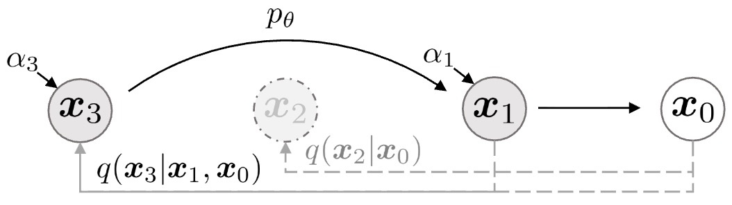
Implementation Details
-
Forward Process (Identical to DDPMs):
-
The forward diffusion process in DDIMs is exactly the same as in DDPMs. Gaussian noise is added to the data over \(T\) discrete timesteps according to:
\[q(x_t \mid x_{t-1}) =N\left( x_t; \sqrt{1 - \beta_t}x_{t-1}, \beta_t I \right)\]-
where:
- \(q(x_t \mid x_{t-1})\) is the forward diffusion transition distribution from timestep \(t-1\) to \(t\).
- \(x_{t-1}\) is the data sample at timestep \(t-1\).
- \(x_t\) is the noisy sample at timestep \(t\).
- \(\beta_t\) is the variance schedule coefficient controlling the noise magnitude at timestep \(t\).
- \({\beta_t}_{t=1}^T\) is the predefined variance schedule across timesteps.
- \(I\) is the identity covariance matrix.
- \(N(\cdot;\mu,\Sigma)\) denotes a multivariate Gaussian distribution with mean \(\mu\) and covariance \(\Sigma\).
- \(T\) is the total number of diffusion steps.
-
-
As in DDPMs, the marginal distribution admits a closed-form expression:
\[x_t =\sqrt{\bar{\alpha}_t},x_0 +\sqrt{1 - \bar{\alpha}_t}\epsilon, \quad \epsilon \sim N(0, I)\]-
where:
- \(x_0\) is the clean data sample.
- \(x_t\) is the noisy data sample at timestep \(t\).
- \(\epsilon\) is standard Gaussian noise.
- \(\epsilon \sim N(0, I)\) denotes sampling noise from a zero-mean unit-variance Gaussian.
- \(\alpha_t = 1 - \beta_t\) is the noise retention factor at timestep \(t\).
- \(\bar{\alpha}_t = \prod_{s=1}^t \alpha_s\) is the cumulative product of retention factors up to timestep \(t\).
- This expression allows sampling of arbitrary timesteps without simulating the full forward chain.
-
-
-
Training Objective (Unchanged from DDPMs):
-
DDIMs require no changes to training. The noise-prediction network is trained using the same DDPM objective:
\[L=\mathbb{E}_{x_0, t, \epsilon} \left[ \left\lVert \epsilon - \epsilon_\theta(x_t, t) \right\rVert^2 \right]\]-
where:
- \(L\) is the training loss.
- \(x_0\) is the clean data sample.
- \(t\) is a timestep sampled uniformly from \({1,\dots,T}\).
- \(x_t\) is obtained by noising \(x_0\) according to the forward process.
- \(\epsilon\) is Gaussian noise with \(\epsilon \sim N(0, I)\).
- \(\epsilon_\theta(x_t, t)\) is the neural network’s prediction of the injected noise.
- \(\mathbb{E}_{x_0,t,\epsilon}[\cdot]\) denotes expectation over data, timesteps, and noise.
-
-
-
Reverse (Implicit) Process:
-
The defining feature of DDIMs is their implicit reverse process, which replaces stochastic sampling with a deterministic update rule. The reverse update is given by:
\[x_{t-1} =\sqrt{\bar{\alpha}_{t-1}} \left(\frac{x_t-\sqrt{1 - \bar{\alpha}_t}\epsilon_\theta(x_t, t)}{\sqrt{\bar{\alpha}_t}}\right) +\sqrt{1 - \bar{\alpha}_{t-1}}\epsilon_\theta(x_t, t)\]-
where:
- \(x_t\) is the sample at timestep \(t\).
- \(x_{t-1}\) is the reconstructed sample at timestep \(t-1\).
- \(\epsilon_\theta(x_t, t)\) is the predicted noise.
- \(\bar{\alpha}_t\) and \(\bar{\alpha}_{t-1}\) are cumulative noise retention coefficients.
- The fraction term estimates the clean sample \(x_0\) from \(x_t\).
- This update corresponds to setting the stochasticity parameter \(\eta = 0\).
-
-
More generally, DDIMs introduce a parameter \(\eta\) that interpolates between deterministic DDIM sampling and stochastic DDPM sampling:
- \(\eta = 0\) \(\rightarrow\) deterministic DDIM
- \(\eta = 1\) \(\rightarrow\) stochastic DDPM
-
-
Sampling:
-
Sampling begins from \(x_T \sim N(0, I)\) and proceeds by applying the deterministic update rule over a subset of timesteps:
\[t_1 > t_2 > \cdots > t_K, \quad K \ll T\]-
where:
- \(x_T\) is the initial pure-noise sample.
- \(N(0,I)\) denotes a standard multivariate Gaussian.
- \(t_1,\dots,t_K\) is a decreasing sequence of selected timesteps.
- \(K\) is the number of sampling steps.
- \(T\) is the total number of diffusion steps.
-
-
By skipping intermediate timesteps and following a non-Markovian trajectory, DDIMs can generate samples in tens of steps rather than hundreds or thousands.
-
Pros
- Dramatically faster sampling than DDPMs.
- Deterministic trajectories enable reproducibility and interpolation.
- No retraining required—fully compatible with DDPM-trained models.
Cons
- Deterministic sampling can reduce sample diversity.
- Excessive timestep skipping can degrade sample quality.
- Still fundamentally discrete-time and tied to a predefined noise schedule.
Latent-Space Diffusion Models
-
Latent-space diffusion models apply the diffusion process in a learned, lower-dimensional representation space rather than directly in the original data space. From a hierarchical standpoint, latent-space diffusion is orthogonal to the time formulation: diffusion in latent space can be implemented using discrete-time objectives (e.g., DDPM-style) or derived from continuous-time SDE formulations.
-
Concretely, an encoder first maps data \(x\) from pixel space into a latent variable \(z\). Diffusion—whether discrete or continuous in time—is then defined over \(z\) using the same Gaussian noising and denoising principles as pixel-space models. Generation proceeds by denoising latent noise and decoding the resulting latent back into data space.
-
In practice, latent-space diffusion has become the dominant paradigm for large-scale generative modeling, particularly for high-resolution image, video, and multimodal generation. Most deployed systems combine:
- latent representations learned via a Variational AutoEncoder (VAE),
- discrete-time DDPM-style noise-prediction objectives, and
- accelerated samplers such as DDIM or probability-flow ODE solvers derived from continuous-time SDE theory.
-
By dramatically reducing the dimensionality of the diffusion space, latent diffusion achieves large gains in computational efficiency while preserving the expressive power and stability of diffusion-based generative modeling.
Latent Diffusion Models (LDMs) / Variational Diffusion Models (VDMs)
-
Latent Diffusion Models (LDMs) apply diffusion processes not in the original data space but in a learned latent representation. This approach was popularized by High-Resolution Image Synthesis with Latent Diffusion Models by Rombach et al. (2022) and directly addresses the primary computational bottleneck of pixel-space diffusion: operating in extremely high-dimensional spaces.
-
While the term Variational Diffusion Models (VDMs) is sometimes used broadly, in modern usage it typically refers to diffusion models combined with a Variational AutoEncoder (VAE), where diffusion is performed in the VAE’s latent space rather than directly on pixels.
-
Within the representation-space axis of the diffusion taxonomy, LDMs should be understood as:
- LDMs are typically discrete-time diffusion models trained with DDPM-style objectives.
- The use of latent space is an implementation and representation choice, not a distinct diffusion family.
- Continuous-time SDE formulations can also be applied in latent space, yielding equivalent generative dynamics under appropriate discretization.
-
LDMs now form the backbone of many modern text-to-image and multimodal systems by combining efficient latent representations with powerful diffusion-based denoising networks.
Implementation Details
-
Latent Representation via a VAE:
-
Latent diffusion models first train a VAE to compress data into a lower-dimensional latent space. Given a data sample \(x\), an encoder produces a latent representation \(z\):
\[z \sim q_\phi(z \mid x)\]-
where:
- \(x\) denotes a data sample in pixel space.
- \(z\) denotes the latent representation.
- \(q_\phi(z \mid x)\) is the encoder distribution.
- \(\phi\) represents the encoder parameters.
- \(\sim\) indicates sampling from the distribution.
-
-
A decoder reconstructs the data via:
\[x \sim p_\theta(x \mid z)\]-
where:
- \(p_\theta(x \mid z)\) is the decoder (likelihood model).
- \(\theta\) represents decoder parameters.
- \(x\) is the reconstructed data sample.
- \(z\) is the latent code.
-
-
The VAE is trained by maximizing the evidence lower bound (ELBO):
\[\mathbb{E}_{q_\phi(z \mid x)} \left[ \log p_\theta(x \mid z) \right] -D_{KL} \left( q_\phi(z \mid x) \mid\mid p(z) \right)\]-
where:
- \(\mathbb{E}_{q_\phi(z \mid x)}[\cdot]\) denotes expectation over encoder samples.
- \(\log p_\theta(x \mid z)\) measures reconstruction likelihood.
- \(D_{KL}(\cdot \mid\mid \cdot)\) denotes Kullback–Leibler divergence.
- \(p(z)\) is the latent prior.
- \(p(z)=N(0,I)\) in practice.
-
The objective balances reconstruction accuracy and regularization toward the prior.
-
-
-
Diffusion in Latent Space (Discrete-Time Formulation):
-
After VAE training, a diffusion process is defined over latent variables using a discrete-time forward process identical in form to pixel-space DDPMs:
\[q(z_t \mid z_{t-1}) =N\left( z_t; \sqrt{1 - \beta_t},z_{t-1}, \beta_t I \right)\]-
where:
- \(q(z_t \mid z_{t-1})\) is the forward latent diffusion transition.
- \(z_{t-1}\) is the latent at timestep \(t-1\).
- \(z_t\) is the latent at timestep \(t\).
- \(\beta_t\) is the noise variance at timestep \(t\).
- \({\beta_t}_{t=1}^T\) is the noise schedule.
- \(I\) is the identity covariance matrix.
- \(T\) is the total number of diffusion steps.
-
Noise magnitude increases with \(t\).
-
-
The corresponding marginal distribution is:
\[z_t =\sqrt{\bar{\alpha}_t},z_0 +\sqrt{1 - \bar{\alpha}_t},\epsilon, \quad \epsilon \sim N(0, I)\]-
where:
- \(z_0\) is the original latent encoding of data.
- \(\epsilon\) is standard Gaussian noise.
- \(\alpha_t = 1-\beta_t\).
- \(\bar{\alpha}_t = \prod_{s=1}^t \alpha_s\).
-
This allows direct sampling of arbitrary timesteps without simulating the full chain.
-
-
-
Training Objective (DDPM-Style Noise Prediction):
- A neural network is trained to reverse the latent diffusion process using the same objective as pixel-space DDPMs (i.e., learning to predict the noise added at each timestep):
-
where:
- \(L\) is the training loss.
- \(\epsilon_\theta(z_t,t)\) is the network’s predicted noise.
- \(\theta\) are denoiser parameters.
- \(t\) is sampled uniformly from \({1,\dots,T}\).
- \(\| \cdot \|^2\) denotes squared Euclidean norm.
-
Because the latent space is much lower dimensional than pixel space, both training and sampling are substantially more efficient.
-
Sampling and Decoding:
- Sampling begins from latent noise:
- Reverse diffusion produces a clean latent \(z_0\), which is decoded into pixel space:
- The decoder maps the denoised latent back into the data space, producing the final sample.
-
As shown in the illustration below from High-Resolution Image Synthesis with Latent Diffusion Models by Rombach et al., the latent representation undergoes \(T\) diffusion steps, after which a U-Net denoiser operates over the noisy latent. Conditioning on text or other modalities is typically implemented via concatenation or cross-attention.
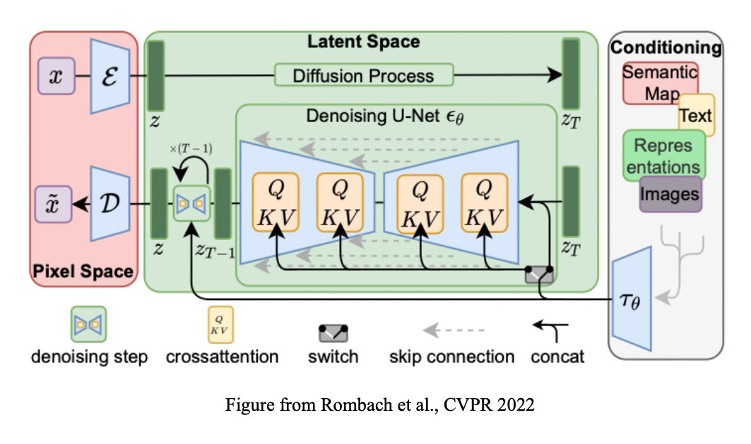
Pros
- Dramatically reduces computational and memory costs compared to pixel-space diffusion.
- Enables efficient high-resolution and multimodal generation.
- Retains the expressive power and stability of discrete-time diffusion models.
Cons
- Overall sample quality depends on the quality of the learned latent representation.
- Introduces additional complexity due to the VAE training stage.
- Reconstruction errors from the VAE can limit ultimate fidelity.
Continuous-Time Diffusion Models (Representation-Agnostic)
-
Continuous-time diffusion models formulate generative modeling as the evolution of data under a continuous-time dynamical process, rather than as a finite sequence of discrete noise steps. In this setting, diffusion is parameterized by a continuous time variable \(t \in [0,1]\), and both the forward (noising) and reverse (generation) processes are described using SDEs.
-
This perspective was unified and formalized in Score-Based Generative Modeling through Stochastic Differential Equations by Song et al. (2021), which showed that many seemingly distinct generative models—including DDPMs, DDIMs, and score-based models—can be understood as different discretizations or solver choices applied to the same underlying continuous-time formulation.
-
From a taxonomy standpoint, continuous-time diffusion models serve as a representation-agnostic and time-continuous generalization of discrete-time diffusion models:
- Pixel-space diffusion models correspond to applying these dynamics directly in data space.
- Latent-space diffusion models correspond to applying the same dynamics in a learned latent representation.
- Score-Based Generative Models (SGMs) correspond to learning the score function required to reverse the diffusion process.
-
Importantly, continuous-time diffusion does not prescribe:
- Where diffusion occurs (pixel space versus latent space), nor
- How the reverse process is parameterized (noise prediction, score prediction, or velocity prediction).
-
Instead, it provides a unifying mathematical framework in which these modeling choices can be rigorously related.
-
In modern systems, continuous-time diffusion primarily functions as a conceptual and theoretical backbone. Practical implementations often rely on discrete-time training objectives (e.g., DDPM-style losses) and fast samplers (e.g., DDIM or ODE solvers) that are derived from this framework.
Stochastic Differential Equation (SDE)-Based Diffusion Models
- SDE-based diffusion models define the forward noising process as a continuous-time stochastic process and the reverse generative process as its time reversal. This framework unifies Denoising Diffusion Probabilistic Models (DDPMs), Denoising Diffusion Implicit Models (DDIMs), and Score-Based Generative Models (SGMs) within a single mathematical formulation, as shown in Score-Based Generative Modeling through Stochastic Differential Equations by Song et al. (2021).
Forward Diffusion as an SDE
-
The forward diffusion process gradually corrupts data by injecting Gaussian noise as time increases. It is defined by the SDE:
\[dx=f(x,t)dt+g(t)dW_t\]-
where:
- \(x\) is the data state at continuous time \(t\).
- \(t\) is the continuous diffusion time variable, typically normalized to \(t \in [0,1]\).
- \(dx\) denotes an infinitesimal change in the state.
- \(f(x,t)\) is the drift term, determining the deterministic evolution of the process.
- \(dt\) is an infinitesimal time increment.
- \(g(t)\) controls the noise magnitude at time \(t\).
- \(dW_t\) is an increment of a standard Wiener (Brownian motion) process.
-
-
A widely used instance is the vVariance-Preserving (VP) SDE:
\[dx=-\frac{1}{2}\beta(t)x dt +\sqrt{\beta(t)}dW_t\]-
where:
- \(\beta(t)\) is a time-dependent noise schedule. The schedule \(\beta(t)\) is chosen so that the marginal distribution transitions smoothly from the data distribution at \(t=0\) to an isotropic Gaussian as \(t \to 1\).
- \(-\frac{1}{2}\beta(t)x\) is the drift term that contracts the signal over time.
- \(\sqrt{\beta(t)}\) scales the stochastic noise injection.
- \(x\) is the data state at time \(t\).
- \(dt\) is an infinitesimal time increment.
- \(dW_t\) is a standard Wiener process increment.
-
-
Discrete-time DDPMs arise as Euler–Maruyama discretizations of this SDE, as shown in Denoising Diffusion Probabilistic Models by Ho et al. (2020).
Score-Based Generative Modeling (SGMs)
-
Score-Based Generative Models are the score-learning instantiation of SDE-based diffusion models. Instead of parameterizing reverse transition kernels directly, SGMs learn the score function which fully specifies the reverse-time dynamics as:
\[s_\theta(x,t) \approx \nabla_x \log p_t(x)\]-
where:
- \(s_\theta(x,t)\) is a neural network parameterized by \(\theta\) that predicts the score.
- \(x\) denotes a data sample or latent variable.
- \(t\) denotes continuous diffusion time.
- \(p_t(x)\) is the marginal probability density of \(x\) at time \(t\).
- \(\nabla_x \log p_t(x)\) is the score, i.e., the gradient of the log-density with respect to \(x\).
- The score function fully specifies the reverse-time dynamics.
-
-
The foundational formulation was introduced in Generative Modeling by Estimating Gradients of the Data Distribution by Song and Ermon (2019) and later generalized to continuous time via SDEs by Song et al. (2021).
Noise-Conditional Perturbation
-
SGMs define a continuum of noisy distributions by perturbing clean data:
\[x_\sigma =x_0 +\sigma \epsilon, \quad \epsilon \sim N(0,I)\]-
where:
- \(x_0\) is a clean data sample.
- \(x_\sigma\) is the noisy sample at noise level \(\sigma\).
- \(\sigma\) is a continuous noise scale controlling perturbation magnitude.
- \(\epsilon\) is standard Gaussian noise.
- \(\epsilon \sim N(0,I)\) denotes a zero-mean unit-variance Gaussian.
-
-
A neural network \(s_\theta(x,\sigma)\) is trained to approximate the score of the noisy distribution:
\[s_\theta(x_\sigma,\sigma) \approx \nabla_{x_\sigma} \log p_\sigma(x_\sigma)\]-
where:
- \(s_\theta(x_\sigma,\sigma)\) is the predicted score at noise level \(\sigma\).
- \(p_\sigma(x_\sigma)\) is the density of noisy samples at noise scale \(\sigma\).
- \(\nabla_{x_\sigma} \log p_\sigma(x_\sigma)\) is the true score of the noisy distribution.
-
Training via Denoising Score Matching
-
Training is performed using denoising score matching, yielding the objective
\[L=\mathbb{E}_{x_0,\sigma,\epsilon} \left[ \lambda(\sigma) \left\lVert s_\theta(x_\sigma,\sigma) +\frac{\epsilon}{\sigma} \right\rVert^2 \right]\]-
where:
- \(L\) is the training loss.
- \(\mathbb{E}_{x_0,\sigma,\epsilon}[\cdot]\) denotes expectation over data samples, noise scales, and Gaussian noise.
- \(\lambda(\sigma)\) is a noise-dependent weighting function.
- \(\lVert\cdot\rVert^2\) denotes squared Euclidean norm.
- This objective trains the model to recover the score field across continuous noise levels.
-
Reverse-Time SDE and Sampling
-
Given a learned score function, generative samples are obtained by stochastically solving the corresponding reverse-time SDE:
\[dx =\left[f(x,t) -g(t)^2 s_\theta(x,t) \right]dt +g(t) d\bar{W}_t\]-
where:
- \(x\) is the evolving sample.
- \(f(x,t)\) is the drift term of the forward SDE.
- \(g(t)\) is the diffusion coefficient.
- \(dt\) is an infinitesimal time increment.
- \(\bar{W}_t\) denotes reverse-time Brownian motion.
-
-
A deterministic alternative is the probability flow ODE:
\[\frac{dx}{dt} =f(x,t)-\frac{1}{2}g(t)^2 s_\theta(x,t)\]-
where:
- \(\frac{dx}{dt}\) is the time derivative of the sample trajectory.
-
This ODE preserves the same marginal distributions and corresponds to DDIM-style sampling, as shown in Denoising Diffusion Implicit Models by Song et al. (2020).
-
Sampling via Langevin Dynamics (Discrete Approximation)
-
Early SGMs implement stochastic sampling via annealed Langevin dynamics, a discrete approximation of the reverse SDE:
\[x_{k+1} =x_k +\eta s_\theta(x_k,\sigma) +\sqrt{2\eta}z_k, \quad z_k \sim N(0,I)\]-
where:
- \(x_k\) is the sample at iteration \(k\).
- \(x_{k+1}\) is the updated sample.
- \(\eta\) is the step size.
- \(z_k\) is Gaussian noise.
-
-
As \(\sigma\) is gradually annealed from large to small values, sampling transitions from coarse structure formation to fine-grained detail refinement.
Probability Flow ODE (Deterministic Sampling)
-
The same SDE defines an associated probability flow Ordinary Differential Equation (ODE):
\[\frac{dx}{dt} =f(x,t)-\frac{1}{2}g(t)^2 s_\theta(x,t)\]-
where:
- \(x\) is the evolving sample.
- \(t\) denotes continuous diffusion time.
- \(\frac{dx}{dt}\) is the time derivative of the sample trajectory.
- \(f(x,t)\) is the drift term of the forward SDE.
- \(g(t)\) is the diffusion coefficient.
- \(s_\theta(x,t)\) is the learned score function.
- \(\theta\) denotes model parameters.
-
-
Solving this ODE yields deterministic sampling trajectories that:
- are equivalent to DDIM-style sampling in discrete time,
- preserve the same marginal distributions as the stochastic SDE,
- and enable exact likelihood computation under mild regularity conditions.
Flow Matching Models (Deterministic Continuous-Time Generative Models)
-
Flow Matching models constitute a closely related but distinct paradigm within continuous-time generative modeling. Rather than deriving dynamics from an SDE or learning a score function, flow matching directly learns a deterministic vector field that transports samples from a simple base distribution to the data distribution.
-
This approach was introduced in Flow Matching for Generative Modeling by Lipman et al. (2022) and further developed in works such as Conditional Flow Matching by Tong et al. (2023).
Core Idea
-
Flow matching defines a time-dependent vector field \(v_\theta(x,t)\) such that samples evolve according to the ODE:
\[\frac{dx}{dt} =v_\theta(x,t)\]-
where:
- \(v_\theta(x,t)\) is a neural network parameterized by \(\theta\) that outputs the deterministic velocity field.
- \(x\) denotes the evolving sample.
- \(t\) denotes continuous time in the interval \([0,1]\).
- \(\frac{dx}{dt}\) is the time derivative of the sample trajectory.
- The vector field deterministically transports samples along a continuous path.
-
-
Samples are constrained to satisfy the boundary conditions \(x(0) \sim p_{\text{base}}\) (e.g., Gaussian noise) and \(x(1) \sim p_{\text{data}}\).
-
where:
- \(x(0)\) is a sample drawn from the base distribution.
- \(p_{\text{base}}\) is a simple base distribution (commonly standard Gaussian).
- \(x(1)\) is a terminal sample.
- \(p_{\text{data}}\) is the data distribution.
-
-
The model is trained to match the true velocity field of an interpolation between base and data distributions.
Flow Matching Objective
-
A common formulation minimizes a regression loss of the form:
\[L_{\text{FM}} =\mathbb{E}_{x_0,x_1,t} \left[ \left\lVert v_\theta(x_t,t) -\frac{d}{dt}x_t \right\rVert^2 \right]\]-
where:
- \(L_{\text{FM}}\) is the flow matching training loss.
- \(\mathbb{E}_{x_0,x_1,t}[\cdot]\) denotes expectation over base samples, data samples, and time.
- \(x_0\) is a sample from the base distribution.
- \(x_1\) is a sample from the data distribution.
- \(x_t\) is a point along a predefined interpolation path between \(x_0\) and \(x_1\).
- \(\frac{d}{dt}x_t\) is the true velocity of the interpolation path at time \(t\).
- \(\lVert\cdot\rVert^2\) denotes squared Euclidean norm.
-
-
The objective trains the model to match the true velocity field along the interpolation.
Relationship to Diffusion and SGMs
- Flow matching can be seen as learning the probability flow ODE directly, without passing through score estimation.
- Unlike SDE-based diffusion, flow matching is fully deterministic and does not inject noise during sampling.
-
Unlike classical normalizing flows, it does not require tractable Jacobian determinants during training.
- As discussed in A Tutorial on Flow Matching by Lilian Weng (2023), flow matching offers a unifying and often simpler alternative to diffusion-based training while retaining continuous-time expressivity.
Pros
- Unified continuous-time view of diffusion, score-based, and ODE-based models
- Flexible trade-offs between stochastic and deterministic generation
- Representation-agnostic and theoretically principled
- Flow matching avoids stochastic sampling and score estimation
Cons
- Requires numerical ODE/SDE solvers and careful time discretization
- Continuous-time formulations are conceptually more abstract
- Flow matching currently has fewer large-scale empirical benchmarks than diffusion
Comparative Analysis
-
Modern generative models based on diffusion and related continuous-time dynamics are best understood through four closely related architectural paradigms, each emphasizing different trade-offs among fidelity, efficiency, determinism, and theoretical generality:
-
Pixel-space diffusion models operate directly on raw high-dimensional data (e.g., image pixels). They offer strong fidelity and interpretability but are computationally expensive and slow to sample from.
-
Latent-space diffusion models apply diffusion in a learned, lower-dimensional representation of the data. This paradigm dramatically improves scalability and efficiency and underpins most modern large-scale generative systems.
-
Continuous-time diffusion models provide a unifying theoretical framework based on SDEs. This formulation connects discrete-time diffusion, score-based modeling, and ODE-based sampling within a single mathematical view.
-
Flow Matching models describe generative modeling as learning a deterministic continuous-time vector field that transports samples from a simple base distribution to the data distribution. While closely related to continuous-time diffusion, flow matching avoids stochastic noise injection and score estimation, offering an alternative deterministic paradigm.
-
-
These paradigms are not mutually exclusive; rather, they occupy different regions of a shared design space:
- Pixel-space vs. latent-space distinguishes where generation occurs.
- Stochastic vs. deterministic dynamics distinguishes how probability mass is transported.
- Discrete-time vs. continuous-time formulations distinguish how the generative process is parameterized and solved.
-
In practice, state-of-the-art systems combine elements from multiple paradigms. A typical modern pipeline uses latent representations for efficiency, DDPM-style discrete-time objectives for stable training, continuous-time theory (via SDEs or ODEs) for principled interpretation and solver design, and—increasingly—deterministic alternatives such as DDIM or flow-matching-style dynamics for fast sampling.
-
This hybrid perspective highlights that modern generative modeling is less about choosing a single model family and more about composing compatible design choices to balance quality, speed, and theoretical clarity.
Pixel-Space Diffusion Models
-
Pixel-space diffusion models apply the generative process directly to high-dimensional data, such as image pixels or raw audio waveforms. In these models, diffusion operates in the original data space, preserving fine-grained details and offering a clear probabilistic interpretation of the generation process.
-
From a design perspective, pixel-space diffusion specifies where the generative dynamics occur, but not how time is parameterized. In principle, pixel-space diffusion can be combined with either discrete-time or continuous-time formulations. Historically and practically, however, pixel-space diffusion models have been dominated by discrete-time stochastic formulations, which established the empirical and conceptual foundation of the field.
-
Pixel-space diffusion models are therefore most naturally organized around discrete-time diffusion, with continuous-time interpretations emerging later as theoretical generalizations rather than as primary implementation choices.
Denoising Diffusion Probabilistic Models (DDPMs)
-
Key idea: Denoising Diffusion Probabilistic Models (DDPMs), introduced in Denoising Diffusion Probabilistic Models by Ho et al. (2020), define a fixed discrete-time forward process that gradually adds Gaussian noise to data, along with a learned reverse Markov chain that removes noise step by step. Generation proceeds by iteratively reversing the diffusion process starting from pure Gaussian noise.
-
In the broader taxonomy, DDPMs:
- are discrete-time diffusion models,
- explicitly parameterize stochastic reverse transitions,
- and operate directly in pixel space.
-
DDPMs form the canonical reference point for diffusion-based generative modeling. Most later developments—including latent diffusion, DDIM sampling, and continuous-time SDE formulations—can be understood as extensions, reinterpretations, or accelerations of this core model.
-
Pros:
- Strong probabilistic grounding with an explicit likelihood
- Stable and well-understood training dynamics
- High-fidelity sample generation
-
Cons:
- Extremely slow sampling due to hundreds or thousands of sequential denoising steps
- Computationally expensive at high resolutions
Denoising Diffusion Implicit Models (DDIMs)
-
Key idea: Denoising Diffusion Implicit Models (DDIMs), proposed in Denoising Diffusion Implicit Models by Song et al. (2020), are sampling procedures rather than new model families. DDIMs reuse the same training objective and learned noise predictor as DDPMs, but replace the stochastic reverse process with deterministic or semi-deterministic trajectories that skip diffusion steps while preserving marginal distributions.
-
Conceptually, DDIMs move pixel-space diffusion toward deterministic continuous-time dynamics, foreshadowing later connections to probability-flow ODEs and flow-based generative perspectives.
-
Pros:
- Orders-of-magnitude faster sampling than DDPMs
- No retraining required
- Deterministic trajectories enable reproducibility and smooth interpolation
-
Cons:
- Aggressive timestep skipping can reduce diversity
- Still constrained by pixel-space computation costs
Relationship to Continuous-Time and Flow-Based Models
-
While DDPMs and DDIMs are formulated in discrete time, both admit continuous-time interpretations:
- DDPMs correspond to numerical discretizations of SDEs.
- DDIMs correspond to deterministic solvers of associated probability-flow ODEs.
-
Pixel-space Score-Based Generative Models and Flow Matching models, which operate directly on pixels but are formulated in continuous time, are therefore best understood as extensions of pixel-space diffusion into the continuous-time regime, rather than as entirely separate pixel-space categories.
-
This perspective highlights pixel-space diffusion as the historical and conceptual starting point from which modern continuous-time and deterministic generative models emerged.
Latent-Space Diffusion Models
-
Latent-space diffusion models apply the generative process in a learned, lower-dimensional representation space rather than directly in pixel space. This latent representation is typically obtained using an autoencoder—most commonly a Variational AutoEncoder (VAE)—which compresses high-dimensional data into a compact and semantically meaningful latent space.
-
From the architectural taxonomy, latent diffusion is a representation-level design choice, orthogonal to the time formulation of the generative process. As a result, latent-space diffusion models can, in principle, be combined with:
- discrete-time stochastic diffusion (e.g., DDPM-style objectives),
- continuous-time stochastic diffusion (via SDEs),
- or deterministic continuous-time dynamics (e.g., probability-flow ODEs or flow-matching-style vector fields).
In practice, however, the vast majority of latent diffusion systems rely on discrete-time DDPM-style training, paired with accelerated samplers derived from continuous-time theory.
Latent Diffusion Models (LDMs)
-
Key idea: Latent Diffusion Models (LDMs), introduced in High-Resolution Image Synthesis with Latent Diffusion Models by Rombach et al. (2022), decouple representation learning from generative modeling. Data are first encoded into a latent variable \(z\), diffusion is applied to \(z\) rather than to pixels, and the final sample is obtained by decoding the denoised latent back into data space.
-
In the broader taxonomy, LDMs:
- specify where generation occurs (latent space),
- typically use discrete-time diffusion objectives for training,
- and often rely on DDIM or ODE-based samplers for efficient inference.
-
This separation dramatically reduces computational cost while preserving the expressive power of diffusion models, enabling high-resolution and multimodal generation at scale.
Advantages of Latent-Space Diffusion
- Computational efficiency: Diffusion operates in a space that is orders of magnitude lower-dimensional than pixel space, significantly reducing memory usage and runtime.
- Scalability: Enables high-resolution image generation and large-scale multimodal systems that would be impractical in pixel space.
- Modularity: The autoencoder and diffusion model can be trained and improved independently.
Limitations and Trade-offs
- Fidelity bound by representation quality: The final sample quality is constrained by the reconstruction accuracy of the autoencoder.
- Additional modeling complexity: Training and maintaining an encoder–decoder pair introduces extra engineering and optimization challenges.
- Approximation error: Latent compression introduces an irreversible information bottleneck.
Relationship to Continuous-Time and Flow-Based Models
-
Latent-space diffusion models can be interpreted within the same continuous-time SDE framework as pixel-space models. Discrete-time latent diffusion objectives correspond to numerical discretizations of latent-space SDEs.
-
Moreover, recent work has explored deterministic latent-space generative dynamics, including probability-flow ODE solvers and flow-matching-style models, which learn continuous-time vector fields directly in latent space.
-
This makes latent diffusion a natural bridge between practical discrete-time diffusion models and deterministic continuous-time approaches, including flow matching, which can further reduce sampling cost by eliminating stochastic noise injection.
Continuous-Time Diffusion Models (Representation-Agnostic)
-
Continuous-time diffusion models describe generative modeling as the evolution of data under a continuous-time dynamical system, rather than a fixed sequence of discrete noise levels. In this paradigm, generation is formulated over a continuous time variable \(t \in [0,1]\), and the transformation from noise to data is governed by either SDEs or ordinary differential equations (ODEs).
-
From the architectural taxonomy, continuous-time diffusion models form a unifying theoretical layer that connects and generalizes discrete-time diffusion models. Importantly, this paradigm is representation-agnostic: the same continuous-time formulation applies whether generation is performed in pixel space, latent space, or another learned representation.
-
Within this framework:
- Discrete-time DDPMs arise as numerical discretizations of specific SDEs.
- DDIM sampling corresponds to solving a deterministic ODE (the probability flow ODE) associated with the same SDE.
- Score-Based Generative Models (SGMs) correspond to learning the score function required to solve reverse-time stochastic dynamics.
- Flow Matching models correspond to directly learning a deterministic continuous-time vector field that transports noise to data, bypassing explicit stochastic diffusion.
-
As a result, continuous-time diffusion should be understood not as a competing model family, but as a mathematical foundation that encompasses stochastic diffusion, deterministic diffusion, and flow-based continuous dynamics within a single conceptual framework.
SDE-Based Diffusion Models (Including Score-Based Generative Models)
-
Stochastic Differential Equation (SDE)-based diffusion models were formalized in Score-Based Generative Modeling through Stochastic Differential Equations by Song et al. (2021). This work showed that learning the score function of noisy data distributions is sufficient to define a valid generative process in continuous time.
-
In this formulation, the forward diffusion process is defined by an SDE of the form:
- where \(W_t\) denotes a standard Wiener process. The forward SDE progressively transforms data into noise, while generation corresponds to solving the associated reverse-time SDE, which depends explicitly on the learned score function:
-
This perspective unifies several previously distinct approaches:
- DDPMs correspond to discretizations of variance-preserving SDEs.
- Langevin-based SGMs correspond to stochastic numerical solvers of the reverse-time SDE.
- DDIM-style samplers correspond to deterministic solvers of the associated probability flow ODE.
-
The key insight is that the score function is the central learned object. Once the score is known, both stochastic and deterministic sampling trajectories are fully specified.
Deterministic Dynamics and Probability Flow ODEs
- Every SDE used in diffusion modeling admits an associated probability flow ODE, which shares the same marginal distributions as the stochastic process but evolves deterministically:
-
Solving this ODE yields deterministic trajectories from noise to data that:
- recover DDIM-style sampling in discrete time,
- eliminate stochastic noise injection during sampling,
- and enable exact likelihood computation under mild regularity conditions.
-
This deterministic view of diffusion provides a conceptual bridge between stochastic diffusion models and fully deterministic continuous-time generators.
Flow Matching Models (Deterministic Continuous-Time Generative Modeling)
-
Flow Matching models represent a closely related but distinct approach to continuous-time generative modeling. Introduced in Flow Matching for Generative Modeling by Lipman et al. (2022), flow matching directly learns a deterministic vector field \(v_\theta(x,t)\) that transports samples from a simple base distribution (e.g., Gaussian noise) to the data distribution.
-
Unlike SDE-based diffusion models, flow matching:
- does not require stochastic forward diffusion,
- does not learn a score function,
- and does not rely on reverse-time stochastic dynamics.
-
Instead, flow matching trains a model to satisfy:
\[\frac{dx}{dt} =v_\theta(x,t)\]-
where \(v_\theta\) is optimized to match a target velocity field defined by pairs of noise and data samples. A common training objective minimizes the mean squared error between the predicted velocity and the target velocity:
\[L_{\text{FM}} =\mathbb{E}_{x_0, x_1, t} \left[ \left\lVert v_\theta(x_t, t) -v^\star(x_t, t) \right\rVert^2 \right]\]
-
-
Flow matching can be viewed as learning the probability flow ODE directly, without passing through an intermediate score or diffusion formulation. As such, it occupies the deterministic end of the continuous-time generative modeling spectrum.
Pros and Cons of Continuous-Time Approaches
-
Pros:
- Provides a unifying theoretical framework for DDPMs, DDIMs, SGMs, and flow matching
- Supports both stochastic (SDE-based) and deterministic (ODE-based) generation
- Representation-agnostic and compatible with pixel-space or latent-space modeling
- Enables flexible trade-offs between sample quality, diversity, and sampling speed
-
Cons:
- Requires numerical solvers and careful step-size or tolerance control
- More abstract than purely discrete-time formulations
- Flow matching models may lack the explicit probabilistic interpretation of diffusion-based likelihoods
Tabular Summary
-
Modern diffusion-based generative models are best understood as configurations within a shared design space, rather than as isolated model families. The primary axes along which these models differ are:
- Representation space: where generation occurs (pixel space vs. latent space)
- Time formulation: whether the generative process is discrete-time or continuous-time
- Generative dynamics: whether sampling is stochastic (noise-injecting) or deterministic
- Learned quantity: noise, score, or velocity field
-
The table below summarizes how the major approaches fit into this taxonomy, including Flow Matching as a distinct deterministic continuous-time paradigm.
| Model / Method | Representation Space | Time Formulation | Sampling Dynamics | Learned Object | Key Trade-offs |
|---|---|---|---|---|---|
| DDPM | Pixel space | Discrete-time | Stochastic (Markovian) | Noise \(\epsilon\) | High fidelity, explicit likelihood, very slow sampling |
| DDIM | Pixel or latent space | Discrete-time | Deterministic / semi-stochastic | Noise \(\epsilon\) | Fast sampling, possible loss of diversity |
| Latent Diffusion (LDM) | Latent space | Discrete-time (typically) | DDIM or ODE-based | Noise \(\epsilon\) | Scalable and efficient, bounded by autoencoder fidelity |
| Score-Based Generative Models (SGMs) | Pixel or latent space | Continuous-time | Stochastic (reverse SDE / Langevin) | Score \(\nabla_x \log p_t(x)\) | Theoretically principled, slow and solver-sensitive |
| SDE-Based Diffusion | Representation-agnostic | Continuous-time | Stochastic (SDE) or deterministic (ODE) | Score \(s_\theta(x,t)\) | Unifying framework, higher conceptual complexity |
| Flow Matching | Pixel or latent space | Continuous-time | Deterministic (ODE) | Velocity field \(v_\theta(x,t)\) | Very fast sampling, weaker probabilistic grounding |
-
Interpretation and Takeaways
- DDPMs define the original discrete-time stochastic diffusion formulation.
- DDIMs are accelerated samplers, not separate models.
- Latent diffusion modifies the representation, not the diffusion theory.
- SGMs are continuous-time, score-learning instantiations of diffusion.
- SDE-based diffusion provides the unifying mathematical framework.
- Flow Matching occupies the deterministic extreme of continuous-time generative modeling, learning transport dynamics directly rather than via noise or score estimation.
-
In practice, modern systems often blend these ideas: latent representations for scalability, DDPM-style objectives for stable training, DDIM or ODE solvers for fast inference, continuous-time theory for interpretation, and—emerging increasingly—flow-matching-style objectives for fully deterministic generation.
Training
- Training diffusion models is grounded in variational inference and aims to learn a parametric approximation to the reverse diffusion process that maximizes the likelihood of observed data. This section presents a high-level yet rigorous view of the training objective, clarifying how likelihood maximization, KL divergences, and simplified denoising objectives fit together, while avoiding overlap with the lower-level derivations covered elsewhere.
- The inference aspect stems from the intractability of the true posterior \(p(x_{0:T}\mid x_0)\), which necessitates inferring a tractable variational distribution \(q_\theta(x_{0:T}\mid x_0)\) by maximizing an ELBO on \(\log p_\theta(x_0)\).
Likelihood Maximization and the Variational Objective
- A diffusion model defines a joint distribution over observed data \(\mathbf{x}_0\) and latent variables \(\mathbf{x}_{1:T}\) through a learned reverse process and a fixed forward noising process. Training seeks to maximize the marginal likelihood of the data:
-
Direct maximization of this likelihood is intractable due to the presence of latent variables. Instead, diffusion models optimize a variational lower bound (ELBO) on the log-likelihood, following the formulation introduced in Deep Unsupervised Learning using Nonequilibrium Thermodynamics by Sohl-Dickstein et al. (2015) and refined in Denoising Diffusion Probabilistic Models by Ho et al. (2020).
-
In practice, training minimizes the negative ELBO, commonly referred to in the diffusion literature as the variational lower bound loss:
\[\mathbb{E}\left[-\log p_\theta(\mathbf{x}_0)\right] \le \mathbb{E}_q \left[ -\log \frac{ p_\theta(\mathbf{x}_{0:T}) }{ q(\mathbf{x}_{1:T} \mid \mathbf{x}_0) } \right] := L_{\mathrm{VLB}}\]-
where:
- \(p_\theta(\mathbf{x}_{0:T})\) is the learned joint distribution defined by the reverse process,
- \(q(\mathbf{x}_{1:T} \mid \mathbf{x}_0)\) is the fixed forward (noising) process,
- \(L_{\mathrm{VLB}}\) is minimized during training.
-
-
Although \(L_{\mathrm{VLB}}\) is technically an upper bound on the negative log-likelihood, the terminology is preserved to remain consistent with the ELBO convention widely used in variational inference literature.
Role of KL Divergences in Diffusion Training
-
A defining advantage of diffusion models is that both the forward and reverse transition distributions are modeled as Gaussian distributions. This allows the variational objective to be decomposed into a sum of Kullback–Leibler (KL) divergence terms, each of which admits a closed-form analytical expression.
-
Expressing the objective in terms of KL divergences provides both theoretical clarity and practical efficiency, as it avoids high-variance Monte Carlo estimators and enables stable optimization.
Recap: KL Divergence
-
The Kullback–Leibler divergence is a fundamental quantity in information theory that measures how one probability distribution diverges from another reference distribution. For continuous distributions, it is defined as:
\[D_{\mathrm{KL}}(P \mid\mid Q) =\int_{-\infty}^{\infty} p(x) \log \left( \frac{p(x)}{q(x)} \right) dx\]-
where:
- \(P\) and \(Q\) are probability distributions over a continuous variable \(x\),
- \(p(x)\) and \(q(x)\) denote their corresponding density functions,
- the logarithmic term compares the relative likelihood assigned by \(P\) and \(Q\) at each point \(x\).
-
-
The KL divergence has several important properties that are directly relevant to diffusion models:
-
Non-negativity: \(D_{\mathrm{KL}}(P \mid\mid Q) \ge 0\), with equality if and only if \(P = Q\) almost everywhere.
- Asymmetry:
\(D_{\mathrm{KL}}(P \mid\mid Q) \neq D_{\mathrm{KL}}(Q \mid\mid P)\) in general.
- This asymmetry reflects the fact that KL divergence measures the inefficiency of using \(Q\) to approximate \(P\), not a symmetric distance between them.
- Information-theoretic interpretation:
- KL divergence quantifies the expected excess code length incurred when encoding samples from \(P\) using a code optimized for \(Q\).
-
-
In diffusion models, this asymmetry is intentional and meaningful: the KL terms penalize discrepancies between the true posterior distributions induced by the forward diffusion process and the learned reverse-time transition distributions.
-
Because these distributions are Gaussian, the KL divergence between them can be computed exactly, which is a key reason diffusion models scale effectively to high-dimensional data.
-
The intuition behind KL divergence is illustrated below. The blue curve represents a varying distribution \(P\), the red curve is a reference distribution \(Q\), and the green curve shows the integrand of the KL expression. The total shaded area corresponds to the KL divergence value.
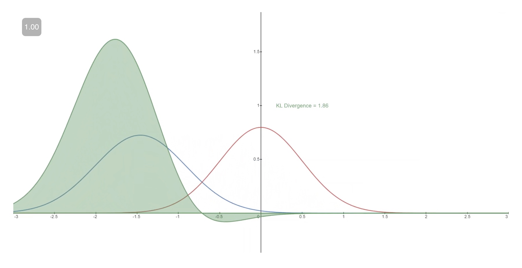
Decomposition of the Variational Lower Bound
-
Leveraging the Markov structure of the diffusion process, the variational loss can be decomposed into a sum of per-timestep terms:
\[L_{\mathrm{VLB}} =L_0 + \sum_{t=1}^{T-1} L_t + L_T\]-
where:
\[\begin{aligned} L_0 &= -\log p_\theta(\mathbf{x}_0 \mid \mathbf{x}_1), \ L_t &= D_{\mathrm{KL}} \big( q(\mathbf{x}_{t} \mid \mathbf{x}_{t+1}, \mathbf{x}_0) \mid\mid p_\theta(\mathbf{x}_{t} \mid \mathbf{x}_{t+1}) \big), \ L_T &= D_{\mathrm{KL}} \big( q(\mathbf{x}_T \mid \mathbf{x}_0) \mid\mid p(\mathbf{x}_T) \big) \end{aligned}\]
-
-
This decomposition, derived in Denoising Diffusion Probabilistic Models by Ho et al. (2020), highlights that:
- all KL terms are analytically tractable,
- the final term \(L_T\) becomes constant when the noise schedule is fixed,
- training primarily focuses on aligning the learned reverse transitions with the true diffusion posteriors.
Simplified Training via Noise Prediction
-
While the full variational objective provides theoretical grounding, Ho et al. (2020) observed that it can be greatly simplified without sacrificing performance.
-
Instead of directly parameterizing reverse transition distributions, the model is trained to predict the noise added during the forward process. This yields a denoising objective closely related to denoising score matching, as formalized in Generative Modeling by Estimating Gradients of the Data Distribution by Song and Ermon (2019).
-
The resulting training objective is:
\[L_{\mathrm{simple}}(\theta) =\mathbb{E}_{\mathbf{x}_0, t, \boldsymbol{\epsilon}} \left[ \left\lVert \boldsymbol{\epsilon} -\boldsymbol{\epsilon}_\theta(\mathbf{x}_t, t) \right\rVert^2 \right]\]- This objective avoids explicit density estimation, yields stable gradients, and empirically matches or exceeds the performance of the full ELBO.
Interpretation and Practical Implications
-
From a training perspective, diffusion models combine:
- a principled likelihood-based foundation,
- a decomposition into closed-form KL divergences,
- and a simple, robust denoising objective used in practice.
-
This balance between theoretical rigor and empirical effectiveness is a central reason diffusion models have become the dominant paradigm in modern generative modeling, as discussed in A Diffusion Model Primer and Diffusion Models Beat GANs on Image Synthesis by Dhariwal and Nichol (2021).
Model Choices
-
With the training objective established, the practical implementation of a diffusion model requires several architectural and design decisions. These choices determine the model’s expressivity, computational efficiency, and sampling behavior. Importantly, diffusion models are unusually flexible: the probabilistic framework places minimal constraints on the neural architecture, requiring only that inputs and outputs share the same dimensionality.
-
This section outlines the major modeling decisions involved in building a diffusion system, focusing on variance scheduling, reverse-process parameterization, and network architecture, while situating these choices within the broader diffusion literature.
Forward Process Design and the Role of the Noise Schedule
-
The forward diffusion process is fixed and non-learned in most practical systems. Its primary design choice is the variance (noise) schedule, which controls how rapidly information is destroyed over time.
-
In discrete-time diffusion models, this schedule is defined by a sequence:
\[{\beta_1, \beta_2, \ldots, \beta_T}\]- where each \(\beta_t\) determines the amount of Gaussian noise added at timestep \(t\).
-
Early diffusion models used simple linear schedules, as proposed in Denoising Diffusion Probabilistic Models by Ho et al. (2020). Later work showed that alternative schedules—such as cosine schedules—improve sample quality and training stability, as demonstrated in Improved Denoising Diffusion Probabilistic Models by Nichol and Dhariwal (2021).
-
Because the forward process is fixed, the KL divergence term associated with the final timestep becomes constant with respect to model parameters. As a result, it does not influence gradient-based optimization and can be ignored during training.
-
In continuous-time formulations, the discrete schedule generalizes to a time-dependent noise rate \(\beta(t)\), preserving the same conceptual role within a SDE framework (cf. Score-Based Generative Modeling through Stochastic Differential Equations by Song et al. (2021)).
Reverse Process Parameterization
-
The reverse diffusion process is learned and defines the generative capacity of the model. Each reverse transition is parameterized as a Gaussian distribution whose parameters are predicted by a neural network.
-
In practice, most diffusion models adopt a restricted covariance parameterization, fixing the covariance to a diagonal matrix determined by the noise schedule. This simplifies optimization and yields stable training, as empirically validated in Denoising Diffusion Probabilistic Models by Ho et al. (2020).
-
Under this design, learning focuses primarily on predicting the mean of the reverse transition, which can be equivalently expressed through alternative parameterizations:
- Noise prediction (predicting \(\epsilon\)),
- Data prediction (predicting \(x_0\)),
- Velocity prediction, introduced in Elucidating the Design Space of Diffusion-Based Generative Models by Karras et al. (2022).
-
Although mathematically equivalent under Gaussian assumptions, these parameterizations differ in numerical stability and empirical performance. Noise prediction remains the most widely used due to its simplicity and robustness.
Neural Network Architectures
-
Diffusion models impose only one structural requirement on the neural network: input and output dimensionalities must match. This flexibility allows a wide range of architectures to be used.
-
In practice, U-Net–style architectures dominate diffusion modeling due to their ability to capture multi-scale spatial structure and propagate information across resolutions. This design choice was popularized in Denoising Diffusion Probabilistic Models by Ho et al. (2020) and refined in subsequent work.
-
Key architectural features commonly employed include:
- multi-resolution convolutional blocks,
- skip connections for stable gradient flow,
- explicit timestep or noise-level embeddings,
- attention layers for long-range dependency modeling.
-
In latent diffusion models, the same architectural principles apply, but diffusion operates on compressed latent representations, as introduced in High-Resolution Image Synthesis with Latent Diffusion Models by Rombach et al. (2022).
Conditioning Mechanisms
-
Many practical diffusion systems are conditional generative models, incorporating auxiliary information such as class labels or text embeddings.
-
Conditioning is typically implemented by injecting additional embeddings into the network via concatenation, cross-attention, or feature-wise modulation. This approach underlies text-to-image systems such as:
- GLIDE by Nichol et al. (2022),
- Imagen by Saharia et al. (2022),
- Stable Diffusion by Rombach et al. (2022).
-
Classifier-free guidance, introduced in Classifier-Free Diffusion Guidance by Ho and Salimans (2022), further improves controllability by interpolating between conditional and unconditional predictions during sampling.
Design Trade-offs
-
The design space of diffusion models is characterized by a clear separation of concerns:
- Forward process: fixed, analytically tractable, defined by a noise schedule.
- Reverse process: learned, parameterized by neural networks.
- Architecture: flexible, with U-Nets as the dominant choice.
- Parameterization: multiple equivalent formulations with different practical properties.
-
This modularity is a key strength of diffusion models, enabling rapid experimentation, theoretical analysis, and integration with emerging frameworks such as continuous-time diffusion and flow-matching models.
Network Architecture: U-Net and Diffusion Transformer (DiT)
-
Diffusion models are a class of generative models that learn to produce high-fidelity data by simulating a noising (forward) and denoising (reverse) process. At a high level, these models include a neural network denoiser that takes in a noisy input at timestep \(t\) and predicts the noise that was added. Because the network must output a tensor of the same shape and spatial resolution as the input image, architectural choices that preserve spatial dimensions and capture both local and global structure are vital.
-
In practice, two dominant architectures have emerged for this denoising network:
- U-Net-based diffusion networks, which rely on spatial convolutions and hierarchical encoding/decoding with skip connections.
- Diffusion Transformers (DiTs), which replace convolutions with attention modules to capture long-range dependencies.
-
Both architectures aim to model the same denoising function:
\[\epsilon_{\theta}(\mathbf{x}_t, t) \approx \epsilon\]- where \(\mathbf{x}_t\) is the noisy image, \(\epsilon\) is the true noise added at step \(t\), and \(\epsilon_{\theta}\) is the network’s prediction.
-
This section describes each architecture in detail, including structural insights and how they are implemented in the context of diffusion models.
U-Net-Based Diffusion Models
-
The canonical implementation for image diffusion models uses U-Net as the backbone denoising network due to its flexibility in processing spatial information across scales. This architecture was adopted in the seminal paper on diffusion models, Denoising Diffusion Probabilistic Models by Jonathan Ho et al. (2020), which demonstrated state-of-the-art image generation performance on benchmarks like CIFAR-10 and LSUN.
-
Key architectural elements of U-Net:
-
Encoder–Decoder Structure: U-Net consists of a sequence of downsampling (encoder) layers that progressively reduce spatial resolution and increase feature abstraction, followed by a symmetric sequence of upsampling (decoder) layers that reconstruct the original resolution. This structure facilitates effective multiscale feature extraction.
-
Skip Connections: Direct connections between corresponding encoder and decoder layers pass fine-grained feature maps forward. This mitigates information loss during downsampling and enables precise reconstruction during upsampling. This bypassing of bottleneck information is critical for high-quality image reconstruction.
-
Bottleneck Layer: The central bottleneck compresses the learned representation and helps the model focus on essential features that are robust to noise, serving as a compact summary of the input.
-
Residual Blocks & Time Embedding: Modern U-Net variants used in diffusion models often incorporate ResNet-like blocks with time and class conditioning embedded into the network via sinusoidal or learned embeddings, enabling the model to reason about temporal noise levels.
-
Because the denoiser must predict noise at each diffusion step, the output of a U-Net takes the same dimensions as the input most of the time:
- This is a key structural constraint that drives the choice toward architectures preserving spatial size.
-
-
Loss Function in U-Net Diffusion:
-
In DDPM training, the network is trained with a simple Mean-Squared Error (MSE) loss between the predicted noise and actual noise:
\[L_{\text{simple}}(\theta)=\mathbb{E}_{t,\mathbf{x}_0,\epsilon}\left[\lVert \epsilon - \epsilon_{\theta}(\mathbf{x}_t,t)\rVert^2\right]\]-
where:
\[\mathbf{x}_t = \sqrt{\bar{\alpha}_t},\mathbf{x}_0 + \sqrt{1-\bar{\alpha}_t}\epsilon\]- with \(\bar{\alpha}_t\) a noise schedule that determines how much noise is added at step \(t\).
-
-
This loss encourages the U-Net to predict the true Gaussian noise component added at each diffusion step.
-
Diffusion Transformer (DiT)
-
While U-Nets excel at capturing local spatial structure, self-attention mechanisms introduced by transformer models can capture long-range dependencies across the image. Scalable Diffusion Models with Transformers by Peebles et al. (2022) introduced DiTs, a family of architectures that replaces the U-Net backbone with transformer blocks to process images in a tokenized or patchified manner.
-
Key features of DiTs include:
-
Patchify and Tokenize: Images are split into patches (similar to Vision Transformers), flattened, and embedded into a sequence of tokens that can be processed by transformer layers.
-
Multi-Head Self-Attention: Each transformer layer employs multi-head attention to aggregate context across all tokens, enabling the model to inherently reason about interactions between distant spatial locations.
-
Feed-Forward Modules: After attention, Feed-Forward Networks (FFNs) apply nonlinear transformations to the attention outputs, enhancing representational capacity.
-
Conditioning for Time and Labels: Additional learned positional embeddings and timestep embeddings are concatenated or added to patch tokens to condition the transformer on the diffusion step and optional class labels.
-
-
DiTs generalize the idea that diffusion models can be implemented with attention-based backbones, showing competitive or superior performance to convolutional U-Nets on high-resolution benchmarks, especially when models are scaled up.
-
Loss Function in DiTs:
-
The objective for DiTs remains analogous to U-Net diffusion:
\[L_{\text{DiT}}(\theta)=\mathbb{E}_{t,\mathbf{x}_0,\epsilon} \left[\lVert \epsilon - \epsilon_{\theta}(\mathbf{x}_t,t)\rVert^2\right]\]- where \(\epsilon_{\theta}\) is now parameterized by a transformer architecture trained to predict noise from a sequence of patch tokens.
-
Comparison Between U-Net and Diffusion Transformer (DiT) Architectures
-
While both U-Net-based models and DiTs are trained to approximate the same denoising function in diffusion models, they differ substantially in their inductive biases, computational characteristics, and scaling behavior. These differences have important implications for model performance, training efficiency, and applicability across data modalities.
-
At a high level, both architectures aim to learn:
\[\epsilon_{\theta}(\mathbf{x}_t, t) \approx \epsilon\]- but the way spatial and contextual information is processed differs significantly.
Inductive Bias and Representation Learning
-
U-Net architectures introduce a strong spatial inductive bias through convolutional operations. Convolutions assume locality and translation invariance, which aligns well with the statistics of natural images. This makes U-Nets particularly effective at modeling fine-grained texture and local structure, even with limited data.
-
This inductive bias was leveraged in Denoising Diffusion Probabilistic Models by Ho et al. (2020), where a convolutional U-Net achieved high-quality image generation without requiring massive datasets or model sizes.
-
In contrast, Diffusion Transformers remove most spatial assumptions and instead rely on self-attention to learn relationships directly from data. Each token can attend to every other token, allowing the model to capture global dependencies explicitly. This design follows the philosophy of transformers introduced in Attention Is All You Need by Vaswani et al. (2017), and adapted to diffusion models in Scalable Diffusion Models with Transformers by Peebles et al. (2022).
-
Formally, self-attention computes:
\[\text{Attention}(Q,K,V) = \text{softmax}\left(\frac{QK^\top}{\sqrt{d_k}}\right)V\]- allowing DiTs to model long-range spatial correlations that convolutional filters must approximate hierarchically.
Model Complexity and Parameter Scaling
-
A major practical difference lies in how computational complexity scales with input size.
- U-Net Complexity:
-
Convolutional layers scale approximately linearly with the number of pixels:
\[\mathcal{O}(HWCk^2)\]- where \(H\), \(W\), and \(C\) denote image height, width, and channels, and \(k\) is the kernel size. This makes U-Nets efficient for high-resolution images.
-
- DiT Complexity:
-
Self-attention scales quadratically with the number of tokens:
\[\mathcal{O}(N^2 d)\]- where \(N\) is the number of image patches and \(d\) is the embedding dimension. As image resolution increases, this cost grows rapidly, motivating patch-based representations and large-scale compute.
-
- Despite this cost, Scalable Diffusion Models with Transformers by Peebles et al. (2022) show that DiTs scale more predictably with model size and dataset size, similar to large language models, often surpassing U-Nets when trained at sufficient scale.
Training Stability and Optimization
-
U-Net-based diffusion models are generally easier to train due to:
- Well-understood convolutional behavior
- Stable gradient flow from skip connections
- Fewer hyperparameters tied to sequence modeling
-
As a result, they are often preferred in low-resource or rapid-iteration settings, such as early research prototyping or smaller datasets.
-
DiT models, on the other hand, require more careful optimization strategies. Training typically involves:
- Large batch sizes
- Learning-rate warmup schedules
- Gradient clipping
- Weight initialization tuned for transformers
-
These techniques mirror best practices from transformer training, as discussed in Scalable Diffusion Models with Transformers by Peebles et al. (2022).
Flexibility Across Modalities
-
A key advantage of DiTs is their architectural generality. Because transformers operate on sequences rather than grids, DiTs can be adapted to:
- Images
- Videos
- Point clouds
- Multimodal representations
-
U-Nets, by contrast, are most naturally suited for grid-structured data such as images and volumetric inputs.
-
This flexibility aligns DiTs with a broader trend toward foundation diffusion models, where a single architecture can be reused across domains, similar to the role of transformers in NLP and multimodal learning.
Trade-offs
-
U-Net diffusion models excel at:
- Efficient high-resolution image generation
- Stable training with limited data
- Strong spatial inductive bias
-
DiTs excel at:
- Modeling global dependencies
- Scaling with data and model size
- Generalization across modalities
-
Both architectures optimize essentially the same diffusion loss:
\[L(\theta) = \mathbb{E}_{t,\mathbf{x}_0,\epsilon} \left[\lVert \epsilon - \epsilon_{\theta}(\mathbf{x}_t,t)\rVert^2\right]\]- but differ in how \(\epsilon_{\theta}\) is parameterized and learned.
Reverse Process of U-Net-Based Diffusion Models
- The reverse (denoising) process is the core generative mechanism in diffusion models. Starting from pure Gaussian noise, the model iteratively applies learned conditional distributions to gradually recover a clean image. This formulation is introduced and formalized in Denoising Diffusion Probabilistic Models by Ho et al. (2020), which defines the reverse process as a learned approximation to the true posterior of the forward noising process.
Markovian Reverse Diffusion Process
-
The forward process is defined as a fixed Markov chain that adds Gaussian noise at each timestep:
\[q(\mathbf{x}_t \mid \mathbf{x}_{t-1}) = \mathcal{N}\left(\mathbf{x}_t; \sqrt{1-\beta_t},\mathbf{x}_{t-1}, \beta_t \mathbf{I}\right)\]- where \(\beta_t \in (0,1)\) is a variance schedule.
-
The reverse process is parameterized as another Markov chain:
\[p_\theta(\mathbf{x}_{t-1} \mid \mathbf{x}_t) = \mathcal{N}\left(\mathbf{x}_{t-1}; \mu_\theta(\mathbf{x}_t,t), \Sigma_\theta(\mathbf{x}_t,t)\right)\]- where the mean \(\mu_\theta\) is learned using a U-Net denoiser, and the variance \(\Sigma_\theta\) is often fixed or learned depending on the variant. This parameterization is derived from the variational framework introduced in Variational Diffusion Models by Kingma et al. (2021).
Noise Prediction Parameterization
-
Instead of directly predicting \(\mu_\theta\), Denoising Diffusion Probabilistic Models by Ho et al. (2020) showed that predicting the noise \(\epsilon\) yields superior empirical performance. Given:
\[\mathbf{x}_t = \sqrt{\bar{\alpha}_t}\mathbf{x}_0 + \sqrt{1-\bar{\alpha}_t}\epsilon\]- the network is trained to predict \(\epsilon_\theta(\mathbf{x}_t,t)\), and the mean is reconstructed as:
-
This reparameterization simplifies training and leads to the widely used noise-prediction objective.
Discrete Likelihood at the Final Reverse Step
-
At the final timestep \(t=1\), the model must map a continuous Gaussian distribution back to a discrete image space, since images consist of integer-valued pixels. This discretization step is crucial for computing the exact likelihood term in the variational lower bound.
-
Following Denoising Diffusion Probabilistic Models by Ho et al. (2020), the reverse distribution for the final step is defined as:
\[p_\theta(\mathbf{x}_0 \mid \mathbf{x}_1) =\prod_{i=1}^{D} p_\theta(x_0^i \mid x_1^i)\]- where \(D\) is the total number of pixels (including channels).
-
Each pixel is modeled using a univariate Gaussian:
\[\mathcal{N}\left(x;\mu_\theta^i(\mathbf{x}_1,1),\sigma_1^2\right)\]- which arises from the diagonal covariance assumption:
Bucket-Based Discretization of Pixel Values
- Images are assumed to be integers in \({0,\dots,255}\), linearly scaled to \([-1,1]\). For a scaled pixel value \(x\), probability mass is assigned by integrating the Gaussian over a small interval:
-
Thus, the probability of a pixel value is:
\[p_\theta(x_0^i \mid x_1^i) =\int_{\delta_-(x_0^i)}^{\delta_+(x_0^i)} \mathcal{N}\left(x;\mu_\theta^i(\mathbf{x}_1,1),\sigma_1^2\right)dx\]-
where:
\[\delta_-(x)= \begin{cases} -\infty & x=-1 \\ x-\frac{1}{255} & x>-1 \end{cases} \quad \delta_+(x)= \begin{cases} \infty & x=1 \\ x+\frac{1}{255} & x<1 \end{cases}\]
-
-
The full likelihood becomes:
Visualization of Discrete Likelihood Buckets
- The following figure illustrates the discretization process. The red curve shows a Gaussian distribution for a pixel at timestep \(t=1\), while the shaded regions represent probability mass assigned to discrete pixel values at (\(t=0\)).
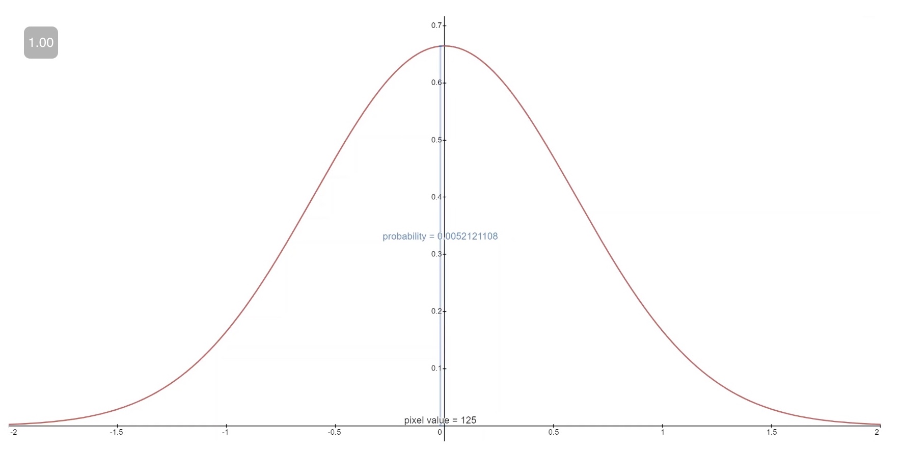
- The first and last buckets extend to \(-\infty\) and \(+\infty\), ensuring that the total probability mass sums to one.
Contribution to the Variational Lower Bound
- This discrete likelihood term forms the only component of the variational lower bound that is not a KL divergence:
-
The full training objective, known as the variational lower bound (VLB), is derived in Denoising Diffusion Probabilistic Models by Ho et al. (2020) and later refined in Improved Denoising Diffusion Probabilistic Models by Nichol et al. (2021).
-
Continuing with the next section, expanded in the same style and level of rigor, and consistent with the original writeup. (There were no images originally in this subsection, so none are added or removed.)
Reverse Process of DiT-Based Diffusion Models
- Diffusion Transformer (DiT) models follow the same probabilistic reverse diffusion framework as U-Net-based models, but differ fundamentally in how the denoising function is parameterized. Rather than operating directly on spatial feature maps with convolutions, DiTs use transformer blocks to model global interactions between image regions via self-attention. This approach was introduced in Scalable Diffusion Models with Transformers by Peebles et al. (2022).
Shared Probabilistic Formulation
-
As with all diffusion models, the reverse process is defined as a Markov chain:
\[p_\theta(\mathbf{x}_{t-1} \mid \mathbf{x}_t) =\mathcal{N}\left( \mathbf{x}_{t-1}; \mu_\theta(\mathbf{x}_t,t), \Sigma_\theta(\mathbf{x}_t,t) \right)\]-
where the mean \(\mu_\theta\) is implicitly defined via the model’s noise prediction:
\[\epsilon_\theta(\mathbf{x}_t,t)\]
-
-
The forward process remains unchanged:
\[\mathbf{x}_t =\sqrt{\bar{\alpha}_t}\mathbf{x}_0 +\sqrt{1-\bar{\alpha}_t}\epsilon, \quad \epsilon \sim \mathcal{N}(\mathbf{0},\mathbf{I})\]- as introduced in Denoising Diffusion Probabilistic Models by Ho et al. (2020). The distinction lies entirely in how \(\epsilon_\theta\) is implemented.
Image Tokenization and Latent Representation
-
In DiT models, images are first divided into non-overlapping patches, analogous to Vision Transformers. Given an image \(\mathbf{x}_t \in \mathbb{R}^{H \times W \times C}\), it is split into \(N\) patches of size \(P \times P\), producing a sequence:
\[\mathbf{z}_t \in \mathbb{R}^{N \times d}\]- where \(d\) is the embedding dimension after linear projection.
-
Each patch embedding is augmented with:
- Positional embeddings
- Timestep embeddings
- Optional class embeddings (for class-conditional generation)
-
This design closely follows transformer conditioning strategies introduced in Attention Is All You Need by Vaswani et al. (2017) and adapted for diffusion in Scalable Diffusion Models with Transformers by Peebles et al. (2022).
Transformer-Based Denoising Dynamics
-
The core of the reverse process consists of stacked transformer blocks. Each block applies multi-head self-attention followed by a feed-forward network:
\[\mathbf{H}^{(l+1)} =\text{FFN}\left( \text{MHA}\left(\mathbf{H}^{(l)}\right) \right)\]-
where multi-head attention is defined as:
\[\text{MHA}(Q,K,V) =\text{Concat}(\text{head}_1,\dots,\text{head}_h)W^O\]-
with:
\[\text{head}_i =\text{softmax}\left( \frac{QW_i^Q (KW_i^K)^\top}{\sqrt{d_k}} \right) VW_i^V\]
-
-
-
Through attention, each patch can condition its denoising prediction on all other patches, allowing DiTs to capture global image structure more directly than convolutional architectures. This property becomes especially important at high resolutions, as shown empirically in Scalable Diffusion Models with Transformers by Peebles et al. (2022).
Noise Prediction and Reconstruction
- After passing through the transformer layers, the token sequence is projected back into patch space and unpatchified to reconstruct a full-resolution noise estimate:
-
As in U-Net-based models, this predicted noise is used to compute the reverse mean:
\[\mu_\theta(\mathbf{x}_t,t) =\frac{1}{\sqrt{\alpha_t}} \left( \mathbf{x}_t -\frac{\beta_t}{\sqrt{1-\bar{\alpha}_t}} \epsilon_\theta(\mathbf{x}_t,t) \right)\]- ensuring that DiTs remain fully compatible with standard diffusion samplers such as DDPM and DDIM, as described in Denoising Diffusion Implicit Models by Song et al. (2020).
Training Objective
- Despite the architectural differences, DiT models are trained with the same simplified noise-prediction loss as U-Net diffusion models:
- This objective arises from minimizing a variational bound on the negative log-likelihood, as shown in Denoising Diffusion Probabilistic Models by Ho et al. (2020) and further analyzed in Improved Denoising Diffusion Probabilistic Models by Nichol et al. (2021).
Sampling Behavior and Scaling Properties
-
One of the key findings of Peebles et al. (2022) is that DiTs exhibit smoother and more predictable scaling behavior than U-Nets as model size and dataset size increase. This mirrors trends observed in large language models and suggests that attention-based diffusion architectures may be better suited for foundation-scale generative modeling.
-
However, the quadratic cost of attention imposes practical constraints on resolution and patch size, motivating hybrid approaches and latent-space diffusion methods explored in High-Resolution Image Synthesis with Latent Diffusion Models by Rombach et al. (2022).
Final Objective
- A central contribution of Denoising Diffusion Probabilistic Models by Ho et al. (2020) is the observation that diffusion model training can be significantly simplified by predicting the noise component added at each timestep, rather than directly predicting the clean image or the reverse-process mean. This insight leads to a remarkably simple and stable training objective that underpins most modern diffusion models.
From Variational Lower Bound to Simplified Loss
-
Diffusion models are trained by maximizing a VLB on the data log-likelihood:
\[\log p_\theta(\mathbf{x}_0) \ge -L_{\mathrm{VLB}}\]-
where the VLB decomposes into a sum of KL divergence terms across timesteps and a final reconstruction term:
\[L_{\mathrm{VLB}} =\mathbb{E}_q\left[L_0 +\sum_{t=2}^{T} L_t +L_T \right]\]
-
-
Most terms in this decomposition take the form:
\[L_t =\mathrm{KL} \big( q(\mathbf{x}_{t-1}\mid\mathbf{x}_t,\mathbf{x}_0) \mid\mid p_\theta(\mathbf{x}_{t-1}\mid\mathbf{x}_t) \big)\]- as derived in Denoising Diffusion Probabilistic Models by Ho et al. (2020) and refined in Improved Denoising Diffusion Probabilistic Models by Nichol et al. (2021).
Noise Prediction Parameterization
-
Rather than learning \(\mu_\theta(\mathbf{x}_t,t)\) directly, Denoising Diffusion Probabilistic Models by Ho et al. (2020) reparameterize the reverse-process mean in terms of predicted noise. Using the forward process:
\[\mathbf{x}_t =\sqrt{\bar{\alpha}_t}\mathbf{x}_0 +\sqrt{1-\bar{\alpha}_t}\epsilon, \quad \epsilon \sim \mathcal{N}(\mathbf{0},\mathbf{I})\]- the model is trained to predict \(\epsilon\) via \(\epsilon_\theta(\mathbf{x}_t,t)\).
-
Under this parameterization, minimizing the KL terms in the VLB becomes (up to constants and weighting factors) equivalent to minimizing a simple mean-squared error loss on the noise:
- This simplification is one of the key reasons diffusion models are stable and easy to train in practice.
The Simple Objective
- Putting everything together, the final training objective used in DDPMs is:
-
This objective:
- Avoids explicit KL divergence computation
- Does not require modeling pixel likelihoods at intermediate timesteps
- Works uniformly across U-Net and DiT architectures
-
The same loss is used in later diffusion variants, including Denoising Diffusion Implicit Models by Song et al. (2020) and Scalable Diffusion Models with Transformers by Peebles et al. (2022).
Training and Sampling Algorithms
-
Training alternates between:
- Sampling a clean image \(\mathbf{x}_0\)
- Sampling a timestep \(t \sim \text{Uniform}({1,\dots,T})\)
- Adding noise to obtain \(\mathbf{x}_t\)
- Updating \(\theta\) to minimize \(L_{\text{simple}}\)
-
Sampling reverses this process, starting from \(\mathbf{x}_T \sim \mathcal{N}(\mathbf{0},\mathbf{I})\) and iteratively applying \(\mathbf{x}_{t-1} \sim p_\theta(\mathbf{x}_{t-1}\mid\mathbf{x}_t)\) until a clean image is produced.
-
The full procedure is summarized in the following table, reproduced from Denoising Diffusion Probabilistic Models by Ho et al. (2020):
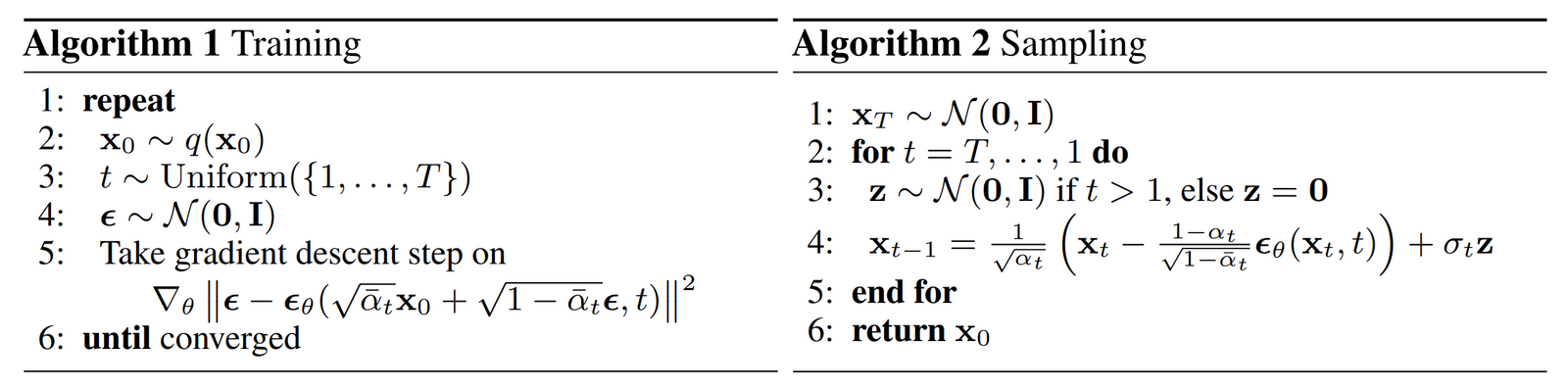
Why This Objective Works
-
Empirically, Denoising Diffusion Probabilistic Models by Ho et al. (2020) show that:
- Noise prediction yields better perceptual quality than predicting \(\mathbf{x}_0\)
- The simplified objective correlates well with likelihood
- The approach generalizes across architectures and datasets
-
This noise-prediction objective has since become the standard loss function for diffusion models, forming the foundation for virtually all modern diffusion-based generative systems.
Key Takeaways
- In summary, U-Net-based diffusion models are the most prevalent type of diffusion models, particularly effective for image-related tasks due to their spatially structured convolutional architecture. They are simpler to train and computationally more efficient. The reverse process in U-Net-based models involves many transformations under continuous conditional Gaussian distributions and concludes with an independent discrete decoder to determine pixel values.
- On the other hand, DiT leverage the power of transformers to handle a variety of data types, capturing long-range dependencies through attention mechanisms. They utilize a series of denoising steps with transformer blocks, employing self-attention mechanisms to effectively model interactions within the data. However, DiT models are more complex and resource-intensive. The reverse process in DiT-based models involves iterative denoising steps using transformer blocks to progressively refine the noisy image.
- The choice between these models depends on the specific requirements of the task, the nature of the data, and the available computational resources.
Conditional Diffusion Models
- Conditional Diffusion Models (CDMs) are an extension of diffusion probabilistic models, where the generation process is conditioned on auxiliary information. This conditioning allows for more structured and controlled synthesis, enabling models to produce outputs that adhere to specific constraints or descriptions.
- Conditioning in diffusion models can be applied using various inputs, such as text (e.g., CLIP embeddings, transformers) or visual data (e.g., images, segmentation maps, depth maps). These inputs influence both the theoretical underpinnings and practical implementations of the models, enhancing their ability to generate outputs aligned with user-defined specifications.
- Early diffusion models relied on simple concatenation techniques for conditioning. However, modern architectures have adopted more sophisticated methods like cross-attention mechanisms, which significantly improve guidance effectiveness. Additionally, techniques such as classifier-free guidance and feature modulation further refine controllability, allowing models to better interpret conditioning signals. These advancements make CDMs powerful tools for diverse tasks, including text-to-image synthesis and guided image manipulation.
Conditioning Mechanisms
-
Diffusion models, which iteratively denoise a Gaussian noise sample to generate an image, can be conditioned by modifying either the forward diffusion process, the reverse process, or both. Below are the primary methods used for conditioning:
-
Concatenation: Directly concatenating conditioning information to the input (e.g., concatenating a text embedding or image feature map to the input image tensor). This was widely used in earlier models such as SR3 (Saharia et al., 2021) and Palette (Saharia et al., 2022).
-
Cross-Attention: Using a transformer-based cross-attention mechanism to modulate the noise prediction process. This is commonly used in modern models like Imagen (Saharia et al., 2022) and Stable Diffusion (Rombach et al., 2022). Importantly, cross-attention is an architectural conditioning mechanism that applies to both U-Net–based diffusion models and Transformer-based diffusion models (DiTs): in U-Nets, convolutional feature maps act as queries attending to conditioning embeddings, while in DiTs, latent tokens act as queries. In both cases, the same attention operation is used:
-
Adaptive Normalization (AdaGN, AdaIN): Using conditioning information to modulate the mean and variance of intermediate activations.
-
Classifier Guidance: Using an external classifier to guide the reverse diffusion process.
-
Score-Based Guidance: Modifying the score function based on conditioning information.
-
-
Below, we describe how these approaches work mathematically and their implementations.
Text Conditioning in Diffusion Models
- Text conditioning in diffusion models typically involves leveraging text encoders such as CLIP, T5, or BERT to obtain a text embedding, which is then integrated into the diffusion model’s denoising network.
Encoding Textual Information
-
A text encoder extracts a fixed-length embedding from an input text description. Suppose the input text is denoted as \(T\), the text encoder \(E_{text}\) produces an embedding:
\[z_T = E_{text}(T) \in \mathbb{R}^{d_{text}}\]- where \(z_T\) is the resulting embedding vector.
Concatenation vs. Cross-Attention Conditioning
- Earlier models such as SR3 (Saharia et al., 2021) and Palette (Saharia et al., 2022) used direct concatenation of conditioning inputs with noise latents. However, modern models like Stable Diffusion and Imagen rely on cross-attention for more expressive conditioning.
Cross-Attention
-
A common method for integrating \(z_T\) into the U-Net-based denoiser is via cross-attention. If \(f_l\) represents the feature map at layer \(l\) of the U-Net, attention-modulated features are computed as:
\[\text{Attention}(Q, K, V) = \text{softmax}\left( \frac{Q K^T}{\sqrt{d}} \right) V\]- where:
-
The U-Net feature maps act as queries, while conditioning embeddings (e.g., text tokens) provide keys and values. This allows the model to attend to relevant text features while generating an image.
Implementation Details (PyTorch)
class CrossAttention(nn.Module):
    def __init__(self, dim, context_dim):
        super().__init__()
        self.to_q = nn.Linear(dim, dim)
        self.to_k = nn.Linear(context_dim, dim)
        self.to_v = nn.Linear(context_dim, dim)
        self.scale = dim ** -0.5

    def forward(self, x, context):
        q = self.to_q(x)
        k = self.to_k(context)
        v = self.to_v(context)
        attn = torch.einsum('b i d, b j d -> b i j', q, k) * self.scale
        attn = attn.softmax(dim=-1)
        out = torch.einsum('b i j, b j d -> b i d', attn, v)
        return out
Visual Conditioning in Diffusion Models
- Visual conditioning can be applied using images, segmentation maps, edge maps, or depth maps as conditioning inputs.
Concatenation-Based Conditioning
-
A simple way to condition on an image is by concatenating it with the noise input at each timestep:
\[x_t' = \text{concat}(x_t, C)\]- where \(x_t\) is the noisy image and \(C\) is the conditioning image.
-
This method was prevalent in early models like SR3.
Feature Map Injection via Cross-Attention
-
More advanced methods use feature injection via cross-attention, as seen in Stable Diffusion and Imagen. Instead of concatenation, this method extracts feature maps from a pretrained encoder \(E_{img}\):
\[z_C = E_{img}(C) \in \mathbb{R}^{h \times w \times d}\]-
and injects these features at various U-Net layers via FiLM (Feature-wise Linear Modulation), which conditions the network by learning per-channel scale and shift parameters that modulate intermediate activations, enabling continuous and fine-grained control without changing spatial resolution:
\[\gamma = W_\gamma(z_C), \quad \beta = W_\beta(z_C)\] \[f_l' = \gamma \odot f_l + \beta\]
-
-
The latent representations from the DiT act as queries, while conditioning embeddings (e.g., text tokens) provide keys and values.
Implementation Details (PyTorch)
class FiLM(nn.Module):
    def __init__(self, in_channels, conditioning_dim):
        super().__init__()
        self.gamma = nn.Linear(conditioning_dim, in_channels)
        self.beta = nn.Linear(conditioning_dim, in_channels)

    def forward(self, x, conditioning):
        gamma = self.gamma(conditioning).unsqueeze(-1).unsqueeze(-1)
        beta = self.beta(conditioning).unsqueeze(-1).unsqueeze(-1)
        return gamma * x + beta
Multi-Modal Conditioning (Text + Image(s) + Other Modalities)
-
Modern Conditional Diffusion Models frequently operate in multi-modal conditioning regimes, where generation is guided simultaneously by multiple sources of information such as text, reference images, depth maps, segmentation masks, human poses, audio, or layout sketches. Rather than treating each modality independently, these systems integrate heterogeneous signals into a unified conditioning space that the denoiser can attend to during generation. This design enables fine-grained controllability, strong spatial faithfulness, compositional editing, and reuse of pretrained diffusion backbones, but it also introduces additional memory overhead, encoder cost, and potential modality-conflict issues that must be managed carefully.
-
This paradigm is central to controllable image synthesis, image-to-image translation, and multimodal generation systems such as:
- High-Resolution Image Synthesis with Latent Diffusion Models by Rombach et al. (2022)
- Imagen: Photorealistic Text-to-Image Diffusion Models by Saharia et al. (2022)
- ControlNet: Adding Conditional Control to Text-to-Image Diffusion Models by Zhang and Agrawala (2023)
- GLIGEN: Open-Set Grounded Text-to-Image Generation by Li et al. (2023)
Unified Multi-Modal Conditioning Representation
-
Assume we have \(M\) modalities, for example:
- Text \(T\)
- Image condition \(C^{(img)}\)
- Depth map \(C^{(depth)}\)
- Segmentation map \(C^{(seg)}\)
-
Each modality is encoded using a specialized encoder:
- To enable joint processing inside the diffusion model, each embedding is projected into a shared conditioning dimension:
- and concatenated into a single conditioning sequence:
- This unified representation allows the denoiser to flexibly attend to whichever modality is most informative at each spatial location or latent token. While concatenation is simple and effective, practitioners must carefully balance embedding sizes to avoid excessive memory consumption.
Cross-Attention with Multiple Modalities
-
Within a diffusion block, conditioning is typically injected using cross-attention:
\[\text{Attn}(Q, K, V)=\text{softmax}\left(\frac{QK^\top}{\sqrt{d}}\right)V\]-
with:
\[Q = W_Q f_l, \quad K = W_K C, \quad V = W_V C\]- where, \(f_l\) denotes intermediate features at layer \(l\) of the denoiser.
-
-
This formulation allows each image region to dynamically combine semantic signals from text with structural information from spatial modalities such as depth or segmentation. The result is strong alignment between prompts and generated content, but cross-attention scales quadratically with conditioning length, motivating aggressive token compression or pooling for large multimodal inputs.
Modality-Specific Injection (ControlNet-Style Conditioning)
-
Some modalities, particularly spatial ones, benefit from feature-level injection rather than token-based attention. ControlNet introduces a parallel network that mirrors the diffusion U-Net and injects features into the main denoiser:
\[f_l' = f_l + g_l(C^{(m)})\]- where \(g_l\) is a modality-specific control branch.
-
Key properties of this approach, introduced in ControlNet: Adding Conditional Control to Text-to-Image Diffusion Models by Zhang and Agrawala (2023):
- The base diffusion model can remain frozen.
- Each modality receives its own lightweight control network.
- Conditioning can be added or removed at inference time.
-
This design yields strong structural fidelity but increases memory footprint due to duplicated network branches.
Spatially Aligned vs. Token-Based Modalities
-
Multi-modal conditioning naturally separates into two categories:
-
Token-Based Modalities
- Text
- Tags
-
Attributes
- These are best injected via cross-attention.
-
Spatially Aligned Modalities
- Depth
- Edges
- Pose
-
Segmentation
- These are often injected via ControlNet branches, FiLM-style modulation, or feature concatenation.
-
Combining both types enables models to achieve both semantic coherence and pixel-level structural control.
Training Objective with Multi-Modal Conditioning
-
The diffusion objective remains unchanged:
\[L=\mathbb{E}_{x_0,t,\epsilon} \left[ \left\lVert \epsilon - \epsilon_\theta(x_t,t,C) \right\rVert^2 \right]\]- where \(C\) now contains multi-modal conditioning. This simplicity is a major advantage: adding modalities does not require modifying the core diffusion loss.
Classifier-Free Guidance with Multi-Modal Inputs
- During training, conditioning signals are randomly dropped on a per-modality basis. At inference:
- This enables smooth trade-offs between adherence to conditioning and sample diversity even when multiple modalities are present.
Practical Capabilities Enabled
-
Multi-modal conditioning supports:
- Text + sketch \(\rightarrow\) image
- Text + depth \(\rightarrow\) photorealistic scene
- Text + bounding boxes \(\rightarrow\) grounded generation (GLIGEN by Li et al. (2023))
- Text + pose \(\rightarrow\) character animation
-
These capabilities illustrate why multi-modal conditioning has become foundational to modern controllable diffusion systems.
Classifier-Free Guidance
Background: Why Are External Classifiers Needed for Text-to-Image Synthesis Using Diffusion Models?
- Diffusion models when used for text-to-image synthesis produce high-quality and coherent images from textual descriptions. However, early implementations of diffusion-based text-to-image models often struggled with aligning generated images precisely with their corresponding textual descriptions. One method to improve this alignment is through classifier guidance, where an external classifier is used to steer the diffusion process. The introduction of an external classifier provided an initial improvement in text-to-image synthesis by guiding diffusion models towards more accurate outputs.
The Need for External Classifiers
- Conditional Control: Early diffusion models generated images by iteratively refining a noise vector but lacked a robust mechanism to ensure strict adherence to the input text description.
- Gradient-Based Steering: External classifiers enabled gradient-based guidance by evaluating intermediate diffusion steps and providing directional corrections to better match the conditioning input.
- Enhancing Specificity: Without an external classifier, models sometimes produced images that, while visually plausible, did not accurately capture the semantics of the input text. The classifier provided a corrective mechanism to reinforce textual consistency.
- Limitations of Pure Unconditional Diffusion Models: Unconditional diffusion models trained without any conditioning struggled to generate diverse yet accurate samples aligned with a given input prompt. External classifiers were introduced to bridge this gap by explicitly providing additional constraints during inference.
Key Papers Introducing External Classifiers for Text-to-Image Synthesis Using Diffusion Models
-
Several papers introduced and explored the use of external classifiers for guiding text-to-image synthesis in diffusion models:
- Dhariwal and Nichol (2021): “Diffusion Models Beat GANs on Image Synthesis”
- This paper introduced classifier guidance as a mechanism to improve the fidelity and control of image generation in diffusion models.
- The approach leveraged an external classifier trained to predict image labels, which was then used to modify the sampling process by influencing the reverse diffusion steps.
- Mathematically, the classifier-based guidance modifies the score function as: \(\nabla_x \log p(y \mid\mid x) \approx \frac{\partial f_y(x)}{\partial x},\) where \(f_y(x)\) represents the classifier’s output logits for class \(y\) given an image \(x\).
- Ho et al. (2021): “Classifier-Free Diffusion Guidance”
- This work proposed classifier-free guidance as an alternative to classifier-based guidance, enabling the model to learn both conditioned and unconditioned paths internally without requiring an external classifier.
- It showed that classifier-free guidance could achieve competitive or superior results compared to classifier-based methods while reducing architectural complexity.
- Ramesh et al. (2022): “Hierarchical Text-Conditional Image Generation with CLIP Latents (DALL·E 2)”
- This paper incorporated a CLIP-based approach to improve text-to-image alignment without directly using an external classifier.
- Instead of an explicit classifier, a pretrained CLIP model was used to guide the image generation by matching textual and visual embeddings.
- Dhariwal and Nichol (2021): “Diffusion Models Beat GANs on Image Synthesis”
How Classifier-Free Guidance Works
- Compared to using external classifiers, classifier-free guidance has since emerged as a more efficient and flexible alternative, eliminating the need for additional classifiers while maintaining or exceeding the performance of classifier-based methods. Put simply, classifier-free guidance provides an alternative to external classifier-based guidance by training the model to handle both conditioned and unconditioned paths internally.
- By incorporating a dual-path training approach and an adjustable guidance scale, classifier-free guidance enhances fidelity, efficiency, and control in text-to-image synthesis, making it a preferred choice in modern generative models.
Dual Training Path
- Conditioned and Unconditioned Paths: During training, the model learns two distinct paths:
- A conditioned path, where the model is trained to generate outputs aligned with a given text description.
- An unconditioned path, where the model generates outputs without any guidance.
- Random Conditioning Dropout: To encourage robustness, the model is trained with random conditioning dropout, where a fraction of inputs are deliberately trained without text guidance.
- Self-Guidance Mechanism: By learning both paths simultaneously, the model can interpolate between conditioned and unconditioned generations, allowing it to effectively control guidance strength during inference.
Equations
- Training Objective:
-
The model learns two score functions:
\[\epsilon_\theta(x_t, y) \text{ and } \epsilon_\theta(x_t, \varnothing)\]- where:
- \(x_t\) is the noised image at time step \(t\),
- \(y\) represents the conditioning input (e.g., text prompt), and
- \(\varnothing\) represents the unconditioned input.
- where:
-
- Guidance During Inference:
-
Classifier-free guidance is implemented as:
\[\tilde{\epsilon}_\theta(x_t, y) = (1 + \gamma) \epsilon_\theta(x_t, y) - \gamma \epsilon_\theta(x_t, \varnothing)\]- where \(\gamma\) is the guidance scale controlling adherence to the conditioning input.
-
- Effect of Guidance Scale:
- When \(\gamma = 0\), the model behaves as an unconditional generator.
- When \(\gamma\) is increased, the generated output aligns more closely with the text condition.
Benefits of Classifier-Free Guidance
- Eliminates the Need for an External Classifier:
- Traditional classifier-based guidance requires a separately trained classifier, adding complexity to both training and inference.
- Classifier-free guidance removes this dependency, simplifying the overall architecture while maintaining strong performance.
- Improved Sample Quality:
- External classifiers introduce additional noise and potential misalignment between the classifier and the generative model.
- Classifier-free guidance directly integrates the conditioning within the diffusion process, leading to more natural and coherent outputs.
- Reduced Computational Cost:
- Training and utilizing an external classifier increases the computational burden.
- Classifier-free guidance eliminates the need for additional model components, streamlining both training and inference.
- Enhanced Generalization and Robustness:
- Classifier-based methods can be prone to adversarial vulnerabilities and overfitting to specific datasets.
- Classifier-free approaches allow the diffusion model to generalize better across different conditioning signals and input variations.
- Flexibility and Real-Time Control:
- Classifier-free guidance allows for dynamic adjustment of the guidance scale \(\gamma\) at inference time, providing fine-tuned control over generation quality and diversity.
- Users can experiment with different \(\gamma\) values without retraining the model, unlike classifier-based methods where the external classifier’s influence is fixed.
Video Diffusion Models
-
Video diffusion models extend image diffusion techniques to sequences by treating videos as spatiotemporal tensors and learning to denoise them across both space and time. This enables a wide range of capabilities, including text-to-video generation, video editing, and image-to-video animation.
-
Notable research in this field includes Imagen Video: High Definition Video Generation with Diffusion Models by Ho et al. (2022), which introduced high-resolution video synthesis from text prompts; Dreamix: Video Diffusion Models are General Video Editors by Molad et al. (2023), which demonstrated robust video editing capabilities using diffusion; and Stable Video Diffusion: Scaling Latent Video Diffusion Models to Large Datasets by Blattmann et al. (2023), which showed how to scale latent video diffusion models effectively.
-
Early approaches in this domain primarily used spatiotemporal U-Nets to jointly model spatial and temporal dimensions. As models scaled and data demands grew, latent-space U-Nets emerged as a more efficient alternative. More recent methods are increasingly leveraging Transformer-based architectures, such as DiTs, to improve scalability and representation learning.
-
Across these architectural variations, the core objective remains the same: to predict noise (or velocity) in a spatiotemporal tensor. The key differences lie in how each model parameterizes and scales this denoising function.
Problem setup
- A video clip is typically represented as a tensor \(x_0 \in \mathbb{R}^{F \times H \times W \times C}\) (frames \(F\), height \(H\), width \(W\), channels \(C\)). “Video diffusion” can be done directly in pixel space (higher fidelity, higher cost) or in a learned latent space (faster and more scalable), with modern systems often favoring latent-space video diffusion (for example, Stable Video Diffusion: Scaling Latent Video Diffusion Models to Large Datasets by Blattmann et al. (2023)).
Training Objective
- Most video diffusion models reuse the same Gaussian noising idea as DDPMs, but applied to the entire spatiotemporal tensor, for discrete timesteps \(t \in {1,\dots,T}\):
-
A convenient closed form is identical in spirit to images:
\[x_t = \sqrt{\bar{\alpha}_t},x_0 + \sqrt{1-\bar{\alpha}_t},\epsilon, \quad \epsilon \sim \mathcal{N}(0,I)\]-
and the standard training loss is the same “noise-prediction MSE,” now over video tensors:
\[L_{\text{video}}(\theta)= \mathbb{E}_{x_0,t,\epsilon} \left[ \left\lVert \epsilon - \epsilon_\theta(x_t,t,\text{cond}) \right\rVert^2 \right]\]-
where:
- \(\beta_t\) is the variance schedule, \(\alpha_t = 1-\beta_t\), and \(\bar{\alpha}_t=\prod_{s=1}^t \alpha_s\) (as in Denoising Diffusion Probabilistic Models by Ho et al. (2020)).
- \(\epsilon_\theta\) is typically a 3D (spatiotemporal) U-Net or a factorized architecture that mixes spatial convolutions with temporal modules, a “natural extension” direction explored in Video Diffusion Models by Ho et al. (2022).
- \(\text{cond}\) denotes conditioning inputs (e.g., text embeddings, an input image, or an input video), with text conditioning prominently used in Imagen Video: High Definition Video Generation with Diffusion Models by Ho et al. (2022).
-
-
Architecture: Spatiotemporal U-Nets and Diffusion Transformers
- Under the hood, most video diffusion systems adapt architectures originally developed for images to operate over space and time, while preserving the core encoder–decoder structure used in diffusion models.
Spatiotemporal U-Net Backbones
-
Early and still widely used video diffusion models extend the 2D U-Net architecture into a 3D or factorized spatiotemporal U-Net, where convolutions and attention operate jointly (or alternately) over spatial and temporal dimensions. This design was introduced and analyzed in Video Diffusion Models by Ho et al. (2022), where the denoiser predicts noise for entire video clips rather than single images.
-
A typical denoiser has the form:
\[\epsilon_\theta(x_t, t, \text{cond})\]-
and is implemented as a multi-scale encoder–decoder with skip connections, where:
- Spatial blocks model per-frame appearance.
- Temporal blocks model motion and inter-frame consistency.
- Cross-attention layers inject conditioning (e.g., text embeddings).
-
-
Formally, intermediate feature maps can be written as:
\[h^{(l+1)} = \text{Block}^{(l)}(h^{(l)}, t, \text{cond})\]- where each block may combine convolution, self-attention, and temporal attention operations.
Latent-Space U-Nets
-
Large-scale systems frequently apply the U-Net in a latent space rather than pixel space, following the paradigm of High-Resolution Image Synthesis with Latent Diffusion Models by Rombach et al. (2022) and extended to video in Stable Video Diffusion: Scaling Latent Video Diffusion Models to Large Datasets by Blattmann et al. (2023). In this setting, an autoencoder first maps videos to latents:
\[z_0 = \mathcal{E}(x_0), \quad x_0 \approx \mathcal{D}(z_0)\]- and diffusion operates on \(z_t\) rather than \(x_t\), greatly reducing computational cost.
Diffusion Transformers (DiTs) for Video
- More recent work explores replacing U-Nets with Transformer-based denoisers, inspired by Scalable Diffusion Models with Transformers by Peebles and Xie (2022). These models treat patches (or latent tokens) as a sequence and apply self-attention across space and time:
- Video extensions tokenize spatiotemporal patches and allow attention to model long-range temporal dependencies more naturally than convolutional stacks. Emerging video systems increasingly adopt hybrid designs combining convolutional stems with Transformer or DiT cores.
Conditioning Pathways
-
Across both U-Net and DiT styles, conditioning (text, image, or video) is typically injected via cross-attention:
\[\text{Attn}(Q, K, V) = \text{softmax}\left(\frac{QK^\top}{\sqrt{d}}\right)V\]- where queries come from video features and keys/values come from conditioning embeddings, as used in Imagen Video: High Definition Video Generation with Diffusion Models by Ho et al. (2022) and Dreamix: Video Diffusion Models are General Video Editors by Molad et al. (2023).
Conditioning and temporal coherence
- Video introduces a key additional constraint beyond images: samples must be temporally coherent (consistent identity, geometry, and motion) while still allowing meaningful dynamics, which motivates architectures and training schemes that explicitly couple frames in time (for example, the joint image-and-video training strategy in Video Diffusion Models by Ho et al. (2022)).
- Text-to-video systems inject text context throughout the denoiser to align motion and appearance with the prompt (as described for the multi-stage cascade in Imagen Video: High Definition Video Generation with Diffusion Models by Ho et al. (2022)).
Cascades and multi-stage generation
- A common strategy for high-resolution video is to generate a low-resolution, low-frame-rate “base” video first, then apply spatial and temporal super-resolution stages, rather than trying to model the full resolution end-to-end.
- Imagen Video is a canonical example: it uses a cascade with interleaved spatial super-resolution (SSR) and temporal super-resolution (TSR) models to reach high resolution and long-ish clips (as summarized in the primer’s Imagen Video notes, and detailed in Imagen Video: High Definition Video Generation with Diffusion Models by Ho et al. (2022)).
- Many modern systems also adopt alternative parameterizations for numerical stability at high resolutions, such as \(v\)-parameterization in Imagen Video: High Definition Video Generation with Diffusion Models by Ho et al. (2022).
Video editing via diffusion
- Beyond pure generation, diffusion models can act as general video editors by combining (i) the original video’s low-frequency spatiotemporal structure with (ii) newly synthesized high-frequency content aligned to a text prompt, sometimes with video-specific finetuning to preserve identity and fidelity.
- Dreamix formalizes this “edit by corrupting then denoising with guidance” approach for real-world videos (as summarized in the primer’s Dreamix notes and introduced in Dreamix: Video Diffusion Models are General Video Editors by Molad et al. (2023)).
Latent video diffusion and scaling
- Latent video diffusion applies diffusion in a compressed representation (often learned by an autoencoder), reducing compute and enabling larger datasets and higher resolutions.
- Stable Video Diffusion emphasizes a staged training recipe (image pretraining, large-scale video pretraining, then high-quality finetuning) and systematic data curation to improve motion representation and generation quality (as summarized in the primer and presented in Stable Video Diffusion: Scaling Latent Video Diffusion Models to Large Datasets by Blattmann et al. (2023)).
Evaluation Metrics
- Evaluating diffusion models requires measuring both sample quality (how realistic individual outputs look) and distributional fidelity (how closely generated samples match the true data distribution), often supplemented by conditioning alignment and human preference studies.
- While image diffusion and video diffusion share several core metrics, video generation additionally requires assessing temporal coherence and motion realism, which motivates specialized spatiotemporal metrics.
Text-to-Image Diffusion Models
-
Text-to-image diffusion models are commonly evaluated using distribution-level statistics computed from deep feature embeddings, along with perceptual and alignment-based measures.
-
Fréchet Inception Distance (FID):
-
The most widely used metric is Fréchet Inception Distance (FID), introduced in GANs Trained by a Two Time-Scale Update Rule Converge to a Local Nash Equilibrium by Heusel et al. (2017). FID compares statistics of real and generated image features extracted from a pretrained Inception network:
\[\text{FID} =\lVert \mu_r - \mu_g \rVert^2 +\text{Tr}\left( \Sigma_r + \Sigma_g - 2(\Sigma_r \Sigma_g)^{1/2} \right)\]-
where:
- \(\mu_r, \Sigma_r\) are the mean and covariance of features from real images,
- \(\mu_g, \Sigma_g\) are the mean and covariance of features from generated images.
-
-
Lower FID indicates closer alignment between generated and real image distributions. FID is standard in diffusion works such as Denoising Diffusion Probabilistic Models by Ho et al. (2020) and High-Resolution Image Synthesis with Latent Diffusion Models by Rombach et al. (2022).
-
-
Inception Score (IS):
- Inception Score (IS), introduced in Improved Techniques for Training GANs by Salimans et al. (2016), measures both sample diversity and confidence of class predictions:
- Higher IS suggests sharper and more diverse images, but IS does not directly compare against real data distributions.
-
Perceptual Similarity Metrics:
- Perceptual metrics compare image pairs in deep feature space, such as LPIPS from The Unreasonable Effectiveness of Deep Features as a Perceptual Metric by Zhang et al. (2018):
- These metrics are often used for image-to-image translation, super-resolution, and reconstruction tasks.
-
Text–Image Alignment Metrics:
- For text-to-image diffusion models, alignment is frequently measured using CLIP-based similarity from Learning Transferable Visual Models From Natural Language Supervision by Radford et al. (2021):
- Higher similarity indicates better semantic alignment between image and prompt.
-
Human Evaluation:
- Because automated metrics are imperfect, many image diffusion papers also report human preference studies measuring realism, fidelity, and alignment.
Text-to-Video Diffusion Models
-
Evaluating text-to-video generation requires measuring both per-frame visual quality and temporal coherence, in addition to distributional similarity.
-
Fréchet Video Distance (FVD):
- Fréchet Video Distance (FVD) was introduced in Video Generation Quality: A Large-Scale Study by Unterthiner et al. (2018) and extends FID to spatiotemporal embeddings:
- Features are extracted using a pretrained video recognition network (e.g., I3D). Lower FVD indicates better video realism. FVD is reported in Video Diffusion Models by Ho et al. (2022) and Imagen Video: High Definition Video Generation with Diffusion Models by Ho et al. (2022).
-
Frame-Level Image Metrics:
- FID and IS are often computed on individual frames, but they do not measure temporal consistency.
-
Temporal Consistency Metrics:
- Temporal smoothness can be assessed via optical-flow consistency or perceptual video similarity metrics inspired by LPIPS, evaluating how features change across adjacent frames.
-
Text–Video Alignment Metrics:
- CLIP-based similarity between text prompts and video frames or pooled video embeddings is used in text-to-video models such as Dreamix: Video Diffusion Models are General Video Editors by Molad et al. (2023).
-
Human Evaluation:
- Human raters assess motion realism, coherence, visual quality, and prompt alignment, and remain the most reliable measure of overall quality.
Prompting Guidance
- Crafting effective prompts is crucial for generating high-quality and relevant outputs using diffusion models. This guide is divided into two main sections: (i) Prompting for Text-to-Image models, and (ii) Prompting for Text-to-Video models.
Prompting Text-to-Image Models
- Text-to-image models, such as Stable Diffusion, DALL-E, and Imagen, translate textual descriptions into visual outputs. The success of a prompt depends on how well it describes the desired image in a structured, caption-like format. Below are the key considerations and techniques for crafting effective prompts for text-to-image generation.
Key Prompting Guidelines
- Phrase Your Prompt as an Image Caption:
- Avoid conversational language or commands. Instead, describe the desired image with concise, clear details as you would in an image caption.
- Example: “Realistic photo of a snowy mountain range under a clear blue sky, with sunlight casting long shadows.”
- Structure Your Prompt Using the Formula:
- [Subject] in [Environment], [Optional Pose/Position], [Optional Lighting], [Optional Camera Position/Framing], [Optional Style/Medium].
- Example: “A golden retriever playing in a grassy park during sunset, photorealistic, warm lighting.”
- Character Limit:
- Prompts must not exceed 1024 characters. Place less important details near the end.
- Avoid Negation Words:
- Do not use words like “no,” “not,” or “without.” For example, the prompt “a fruit basket with no bananas” may result in bananas being included. Instead, use negative prompts:
- Example:
Prompt: A fruit basket with apples and oranges.
Negative Prompt: Bananas.
- Example:
- Do not use words like “no,” “not,” or “without.” For example, the prompt “a fruit basket with no bananas” may result in bananas being included. Instead, use negative prompts:
- Refinement Techniques:
- Use a consistent seed value to test prompt variations, iterating with small changes to understand how each affects the output.
- Once satisfied with a prompt, generate variations by running the same prompt with different seed values.
Example Prompts for Text-to-Image Models
| Use Case | Prompt | Negative Prompt |
|---|---|---|
| Stock Photo | "Realistic editorial photo of a teacher standing at a blackboard with a warm smile." | "Crossed arms." |
| Story Illustration | "Whimsical storybook illustration: a knight in armor kneeling before a glowing sword." | "Cartoonish style." |
| Cinematic Landscape | "Drone view of a dark river winding through a stark Icelandic landscape, cinematic quality." | None |
Prompting Text-to-Video Models
- Text-to-video models extend text-to-image capabilities to temporal domains, generating coherent sequences of frames based on textual prompts. These models use additional techniques, such as temporal embeddings, to capture motion and transitions over time.
Key Prompting Guidelines
- Phrase Your Prompt as a Video Summary:
- Describe the video sequence as if summarizing its content, focusing on the subject, action, and environment.
- Example: “A time-lapse of a sunflower blooming in a sunny garden. Vibrant colors, cinematic lighting.”
- Include Camera Movement for Dynamic Outputs:
- Add camera movement descriptions (e.g., dolly shot, aerial view) at the start or end of the prompt for optimal results.
- Example: “Arc shot of a basketball spinning on a finger in slow motion. Cinematic, sharp focus, 4K resolution.”
- Character Limit:
- Like text-to-image prompts, video prompts must not exceed 1024 characters.
- Avoid Negation Words:
- Use negative prompts to exclude unwanted elements, similar to text-to-image generation.
- Refinement Techniques:
- Experiment with different camera movements, action descriptions, or lighting effects to improve output consistency and realism.
Camera Movements
- In video prompts, describing camera motion adds dynamic perspectives to the generated sequence. Below is a reference table of common camera movements and their suggested keywords:
| Camera Movement | Suggested Keywords | Definition |
|---|---|---|
| Aerial Shot | aerial shot, drone shot, first-person view (FPV) | A shot taken from above, often from a drone or aircraft. |
| Arc Shot | arc shot, 360-degree shot, orbit shot | Camera moves in a circular path around a central point/object. |
| Clockwise Rotation | camera rotates clockwise, clockwise rolling shot | Camera rotates in a clockwise direction. |
| Dolly In | dolly in, camera moves forward | Camera moves forward. |
Example Prompts for Text-to-Video Models
| Use Case | Prompt | Negative Prompt |
|---|---|---|
| Food Advertisement | "Cinematic dolly shot of a juicy cheeseburger with melting cheese, fries, and a cola on a diner table." | "Messy table." |
| Product Showcase | "Arc shot of a luxury wristwatch on a glass display, under studio lighting, with a blurred background." | "Low resolution." |
| Nature Scene | "Aerial shot of a waterfall cascading through a dense forest. Soft lighting, 4K resolution." | None |
Key Takeaways
Text-to-Image
- For text-to-image tasks, focus on describing the subject and its environment with optional details like lighting, style, and camera position. Use clear, concise descriptions structured like image captions.
Text-to-Video
-
For text-to-video tasks, describe the sequence as a whole, including subject actions, camera movements, and temporal transitions. Camera motion plays a critical role in adding dynamic elements to the video output.
-
Both types of prompting require careful attention to phrasing and refinement to achieve optimal results. By iterating and experimenting with different seeds and negative prompts, you can generate visually stunning and contextually accurate outputs tailored to your needs.
Integrating Diffusion Models with an Large Language Model (LLM) Backbone
-
Integrating diffusion models with a Large Language Model (LLM) backbone combines two powerful generative paradigms: LLMs, which excel at discrete symbolic reasoning and sequential semantic processing, and diffusion models, which excel at continuous high-dimensional synthesis. Instead of treating text prompts as static embeddings, this paradigm uses the internal representations or finetuned decoders of LLMs themselves to condition the diffusion process more richly and flexibly. Here is the updated version of the introductory section, with:
-
This approach goes beyond simply using an LLM as a text encoder. It involves finetuned or decoder-oriented LLM architectures that are adapted for use within diffusion conditioning, with the goal of tightly coupling semantic planning and perceptual generation. Recent work in this direction includes:
-
Decoder-Only LLMs are Better Controllers for Diffusion Models by Dong et al. (2025), which explores using modern decoder-only LLM architectures as controllers for diffusion and proposes lightweight projection layers that convert decoder hidden states into diffusion conditioning signals.
-
A Comprehensive Study of Decoder-Only LLMs for Text-to-Image Generation by Wang et al. (2025), which systematically evaluates how decoder-only LLMs can serve as semantic backbones for diffusion-based image generation, including strategies for extracting representations from multiple decoder layers.
-
Large Language Models to Diffusion Finetuning by Cetin et al. (2025), which introduces a finetuning framework that adapts pretrained LLM decoders to leverage diffusion-style iterative refinement while preserving their original autoregressive capabilities.
-
-
Throughout this section, we use the term Projection Layers to refer to the lightweight neural modules that transform LLM hidden states into diffusion-compatible conditioning. In prior literature, similar components are sometimes called adapters, bridges, or interface modules; however, they should not be confused with LoRA-style parameter-efficient adapters, as they serve a different functional role.
-
At a high level, the integrated system can be summarized as:
- Crucially, the diffusion model is not prompted with raw text. Instead, it is conditioned on continuous latent representations produced by the LLM, enabling tighter semantic control, better compositionality, and richer alignment between language and vision.
Overall Architecture
-
An LLM–diffusion system with projection layers is best understood as a three-stage pipeline with clearly separated responsibilities:
- A decoder-oriented LLM responsible for semantic understanding, reasoning, and planning.
- A set of Projection Layers that translate discrete LLM representations into continuous conditioning signals.
- A diffusion generator that transforms noise into perceptual samples under that conditioning.
-
This modular decomposition allows each component to be pretrained independently and later integrated with minimal interference, which is critical for stability and scalability.
LLM Backbone (Semantic Planner)
-
The LLM serves as a semantic planner rather than a perceptual generator. Its role is to transform user text into a sequence of contextual hidden states that encode objects, attributes, relationships, style, and global intent.
-
Typical choices:
- Decoder-only Transformers following the architecture of Attention Is All You Need by Vaswani et al. (2017).
-
Large-scale autoregressive models such as those described in Language Models are Few-Shot Learners by Brown et al. (2020).
-
Implementation details:
- Input prompt is tokenized into \(T\) tokens.
- Forward pass produces hidden states at each layer.
- One or more layers’ outputs are selected (often the final layer or a weighted combination of top layers).
-
Resulting tensor:
\[H \in \mathbb{R}^{T \times d_{\text{LLM}}}\] -
Practical considerations:
- Using intermediate-layer representations sometimes yields better visual grounding than only the final layer.
- Long prompts may be truncated or summarized to control memory usage.
- The LLM may be fully frozen or partially finetuned depending on training strategy.
Projection Layers (LLM \(\rightarrow\) Diffusion Interface)
-
Projection Layers transform LLM hidden states into a form usable by the diffusion model.
-
Their purpose is to:
- Match dimensionality.
- Align semantic axes.
- Control information flow.
-
Baseline linear projection:
\[C = H W + b\]-
where:
\[W \in \mathbb{R}^{d_{\text{LLM}} \times d_{\text{diff}}}\]
-
-
More expressive variants:
- Two-layer MLP with GELU.
- Cross-attention compression block.
- Per-layer projection stacks if conditioning multiple diffusion stages.
-
Implementation details:
- Typically 1–10M parameters.
- Initialized with small variance to avoid destabilizing diffusion.
- Often include LayerNorm before projection.
-
Resulting conditioning tensor:
\[C \in \mathbb{R}^{S \times d_{\text{diff}}}\]- where \(S\) may equal \(T\) or be reduced via pooling or attention.
Diffusion Generator (Perceptual Decoder)
-
The diffusion model is responsible for all pixel synthesis.
-
Common instantiations:
- Latent diffusion U-Net from High-Resolution Image Synthesis with Latent Diffusion Models by Rombach et al. (2022).
- Transformer denoiser from Scalable Diffusion Models with Transformers by Peebles and Xie (2022).
-
Responsibilities:
- Maintain forward noise schedule.
- Predict noise (or equivalent) at each timestep.
- Integrate conditioning through cross-attention or modulation.
-
Practical details:
- Usually frozen initially.
- Sampling performed with DDIM or ODE samplers.
- Runs in latent space for efficiency.
Data Flow During Inference
- User prompt \(\rightarrow\) LLM.
- LLM produces hidden states \(H\).
- Projection Layers compute \(C\).
- Diffusion sampling begins from noise.
- Conditioning injected at every denoising step.
- Final image decoded.
-
This strict separation ensures:
- LLM focuses on semantics.
- Diffusion focuses on perception.
- Projection Layers handle translation.
Engineering Considerations
- Mixed precision (fp16/bf16) throughout.
- Cache LLM hidden states across diffusion steps.
- Projection Layers executed once per sample.
- Diffusion dominates runtime.
Representations Exchanged Between the LLM and Diffusion
- The integration hinge is the representation interface: diffusion models require continuous conditioning signals that can be consumed repeatedly across denoising steps, while decoder LLMs naturally produce token-sequence hidden states optimized for next-token prediction. The goal is to choose what to extract from the LLM, how to package it, and how to make it compatible with the diffusion model’s conditioning pathways.
What the LLM Produces
- Given a tokenized prompt of length \(T\), a decoder LLM produces per-token hidden states (typically from the final layer, though intermediate layers may be used):
-
Implementation detail:
- \(T\) is the number of text tokens after tokenization.
- \(d_{\text{LLM}}\) is the model hidden width (e.g., 1024, 4096, 8192).
- You generally want to extract the hidden states corresponding to the prompt tokens, not logits, because diffusion conditioning is continuous and benefits from rich intermediate representations.
-
Practical variants:
- Use only the final layer hidden states.
-
Use a learned weighted combination of top \(k\) layers:
\[H = \sum_{l=L-k+1}^{L} w_l H^{(l)}, \quad \sum_l w_l = 1\]- which often improves semantic richness and stability when the LLM has been trained primarily for text generation.
What the Diffusion Model Wants
-
Diffusion models commonly accept conditioning in one or more of the following formats:
-
Token-level conditioning for cross-attention:
- A sequence of context vectors used as keys/values.
- This is the most common and flexible scheme in modern systems.
-
Global conditioning vectors:
- One vector that represents overall semantics or style.
-
Spatial conditioning feature maps:
- Useful for visual conditions like depth maps or segmentation, but less common for pure text.
-
-
Because diffusion runs over multiple timesteps, conditioning must be:
- Stable (does not vary with timestep unless explicitly designed to).
- Efficiently reusable (computed once and cached).
- Shaped to match the diffusion architecture.
Projection Layers Output Shapes
- Projection Layers convert LLM representations into diffusion-compatible conditioning:
-
Key design choice is \(S\):
- No compression: set \(S = T\). This retains full prompt granularity but can be expensive if \(T\) is large.
- Compression: set \(S \ll T\) using pooling or attention. This reduces memory and often improves controllability by forcing the model to focus on salient features.
-
Common compression strategies:
-
Mean pooling:
\[c_{\text{global}} = \frac{1}{T}\sum_{i=1}^T H_i\]- and either use as a single-token context \(S=1\) or expand into multiple learned tokens.
-
Learned token bottleneck:
-
Introduce \(M\) learned “diffusion context tokens” \(D \in \mathbb{R}^{M \times d_{\text{LLM}}}\) and compute:
\[C = \text{Attn}(D, H, H)\]- producing \(S=M\) tokens. This is often a strong default when \(T\) is variable or large.
-
-
Matching Dimensions and Normalization
-
Diffusion cross-attention has a fixed context width \(d_{\text{diff}}\). If the diffusion model is a U-Net conditioned via cross-attention, \(d_{\text{diff}}\) is typically the transformer width used in attention blocks. If the diffusion model is a DiT-style denoiser, \(d_{\text{diff}}\) is the token embedding dimension.
-
The simplest mapping is a linear projection:
\[C = H W + b, \quad W \in \mathbb{R}^{d_{\text{LLM}} \times d_{\text{diff}}}\] -
Implementation details that matter in practice:
- Apply LayerNorm to \(H\) before projection to stabilize scale: \(\tilde{H} = \text{LayerNorm}(H).\)
- Initialize \(W\) with small variance to avoid overpowering the diffusion model’s existing conditioning pathways.
- Cache \(C\) so it is computed once per prompt, not per diffusion step.
Multi-Stream Conditioning: “What” vs “How”
-
In many systems it is useful to split conditioning into semantic and stylistic components. A practical implementation is to produce:
- A token sequence \(C_{\text{tokens}} \in \mathbb{R}^{S \times d_{\text{diff}}}\) for cross-attention (“what to draw”).
- A global vector \(c_{\text{global}} \in \mathbb{R}^{d_{\text{diff}}}\) for FiLM or normalization modulation (“how to draw it”).
-
This makes it easier to implement features like:
- Style locking (keep \(c_{\text{global}}\) fixed).
- Layout re-planning (modify \(C_{\text{tokens}}\)).
How This Relates to Decoder-LLM Controllers
- The core idea of using decoder-only LLM representations as a control interface for diffusion is explored in Decoder-Only LLMs are Better Controllers for Diffusion Models by Dong et al. (2025) and studied systematically in A Comprehensive Study of Decoder-Only LLMs for Text-to-Image Generation by Wang et al. (2025), where the central implementation question is exactly this interface: which layers, what compression, and how to project to diffusion conditioning spaces.
Conditioning Injection into the Diffusion Model
-
Once the Projection Layers produce conditioning representations \(C\), the next design question is how and where this conditioning enters the diffusion denoising network. This choice strongly affects controllability, expressivity, computational cost, and training stability.
-
Modern diffusion systems almost always inject conditioning inside the denoiser, rather than modifying the forward noising process. The dominant pattern is to integrate conditioning at multiple depths of the network so that semantic information can influence both global structure and fine-grained details.
Cross-Attention Conditioning (Primary Mechanism)
-
Cross-attention is the most widely used conditioning mechanism in state-of-the-art diffusion systems, including latent diffusion architectures such as High-Resolution Image Synthesis with Latent Diffusion Models by Rombach et al. (2022) and large text-conditioned systems such as Imagen: Photorealistic Text-to-Image Diffusion Models by Saharia et al. (2022).
-
Inside a diffusion block, cross-attention computes:
\[\text{Attn}(Q,K,V) =\text{softmax}\left(\frac{QK^\top}{\sqrt{d}}\right)V\]-
where:
- Queries \(Q\) come from intermediate image or latent features.
- Keys \(K\) and values \(V\) come from conditioning representations \(C\).
-
Where Cross-Attention Is Inserted
-
In U-Net–based denoisers:
- Cross-attention layers are typically placed inside residual blocks.
- Often inserted at mid-resolution and high-resolution stages, where semantic layout and object identity matter most.
- Early low-level convolution blocks may omit conditioning to reduce compute.
-
In Transformer-based denoisers (DiT):
- Each Transformer block naturally supports cross-attention.
- Image/latent tokens attend to conditioning tokens.
Practical Implementation Details
- Conditioning \(C\) is cached and reused at every diffusion timestep.
- Multi-head attention is used.
- Attention dropout is often disabled to preserve conditioning signal.
Why Cross-Attention Works Well
- Allows token-level alignment between words and visual regions.
- Supports variable-length conditioning.
- Enables classifier-free guidance and prompt interpolation.
Prefix Conditioning
-
Prefix conditioning treats \(C\) as a prefix sequence concatenated to the denoiser’s internal token stream before self-attention.
-
This technique is conceptually similar to prefix-tuning in language models and is sometimes used in Transformer denoisers.
-
Advantages:
- Simple integration into Transformer stacks.
- No separate cross-attention block required.
-
Limitations:
- Less explicit control over how strongly conditioning influences features.
- Harder to scale with large conditioning sequences.
-
Because of these drawbacks, prefix conditioning is less common than explicit cross-attention in diffusion.
FiLM-Style Feature Modulation
- Feature-wise Linear Modulation (FiLM), introduced in FiLM: Visual Reasoning with a General Conditioning Layer by Perez et al. (2018), modulates intermediate activations using scale and shift parameters derived from conditioning:
-
Implementation details:
- \(f(\cdot)\) is typically a small MLP.
- Applied after normalization layers.
- Often used alongside cross-attention rather than alone.
-
Use cases:
- Style control.
- Global color palette shifts.
- Lighting or texture modulation.
Combining Multiple Conditioning Pathways
-
High-end systems frequently combine:
- Cross-attention for semantic structure.
- FiLM for global style.
- Optional global vectors for strength control.
-
This multi-pathway design improves disentanglement between what is generated and how it is rendered.
Classifier-Free Guidance Compatibility
-
Cross-attention conditioning naturally supports classifier-free guidance as introduced in Classifier-Free Diffusion Guidance by Ho and Salimans (2022):
- During training, randomly drop conditioning.
-
At inference, combine conditional and unconditional predictions.
- This mechanism depends on conditioning being injected inside the denoiser, which further motivates cross-attention-based designs.
Engineering Considerations
- Memory usage scales with \(S \times d_{\text{diff}}\).
- Long prompts should be compressed.
- Conditioning tensors should remain in GPU memory across timesteps.
- Attention kernels (FlashAttention, xFormers) significantly improve throughput.
Training Strategies
-
Training an LLM–diffusion system with Projection Layers involves deciding which components are frozen, which are trainable, and how gradients flow across modules. These choices strongly affect stability, cost, and final alignment quality. Most practical systems follow a staged or partially frozen strategy rather than full end-to-end training from scratch.
-
At a high level, training always uses the standard diffusion denoising objective, while conditioning is supplied by the LLM through Projection Layers.
Base Objective (Shared Across Strategies)
-
Nearly all diffusion-based image generators use a noise-prediction objective derived from Denoising Diffusion Probabilistic Models by Ho et al. (2020):
\[\mathcal{L}_{\text{diff}} =\mathbb{E}_{z_0,t,\epsilon} \left[ \left\lVert \epsilon - \epsilon_\theta(z_t, t, C) \right\rVert^2 \right]\]-
where:
- \(z_0\) is the clean latent representation.
- \(z_t\) is the noised latent at timestep \(t\).
- \(\epsilon\) is Gaussian noise.
- \(\epsilon_\theta\) is the denoiser prediction.
- \(C\) is conditioning from the Projection Layers.
-
-
All training strategies differ mainly in which parameters receive gradients.
Strategy A: Freeze Diffusion, Train Projection Layers Only
-
This is the most stable and commonly used starting point.
-
Procedure:
- Load a pretrained diffusion model.
- Freeze all diffusion weights.
- Freeze the LLM.
- Train only the Projection Layers.
-
Rationale:
- Diffusion model already knows how to render images.
- Projection Layers learn how to translate LLM semantics into the diffusion conditioning space.
-
Implementation details:
- Optimizer: AdamW.
- Learning rate: 1e-4 to 5e-5.
- Batch sizes similar to standard diffusion fine-tuning.
- Mixed precision strongly recommended.
-
Advantages:
- Very low memory overhead.
- Minimal risk of catastrophic forgetting.
- Easy to debug.
-
Limitations:
- LLM cannot adapt its internal representation for vision.
- Upper bound on alignment quality.
-
This regime is consistent with findings in Decoder-Only LLMs are Better Controllers for Diffusion Models by Dong et al. (2025).
Strategy B: Train Projection Layers + Top LLM Layers
-
To improve semantic grounding, a small number of LLM layers (typically the top 1–4) are unfrozen.
-
Procedure:
- Freeze diffusion.
- Unfreeze Projection Layers.
- Unfreeze last few Transformer blocks of the LLM.
-
Rationale:
- Allows LLM to shape hidden states toward visually meaningful features.
- Still preserves most pretrained language knowledge.
-
Implementation details:
- Use smaller learning rate for LLM (e.g., 1e-5).
- Gradient clipping recommended.
- Often use layer-wise learning rate decay.
-
Advantages:
- Stronger alignment than Strategy A.
- Moderate additional cost.
-
Risks:
- Overfitting on image-caption data.
- Drift in linguistic quality if too many layers are unfrozen.
Strategy C: Partial Joint Fine-Tuning with Diffusion
-
For highest performance, some diffusion parameters are also unfrozen.
-
Typically unfrozen:
- Cross-attention layers.
- Conditioning projection layers inside diffusion blocks.
-
Procedure:
- Freeze most convolutional / transformer weights.
- Unfreeze cross-attention.
- Train Projection Layers and limited LLM layers.
-
Rationale:
- Lets diffusion adapt to new conditioning distribution.
- Improves compositionality and instruction following.
-
Cost:
- Significantly higher GPU memory.
- Slower convergence.
-
This style of partial finetuning is consistent with practices in large text-to-image systems such as Imagen: Photorealistic Text-to-Image Diffusion Models by Saharia et al. (2022).
Classifier-Free Guidance Training
-
To enable classifier-free guidance:
- With probability \(p\), drop conditioning \(C\).
- Replace with learned null embedding.
-
This trains both conditional and unconditional paths in a single model, as introduced in Classifier-Free Diffusion Guidance by Ho and Salimans (2022).
-
Implementation details:
- Typical \(p = 0.1\) to \(0.2\).
- Null embedding is learned vector.
Auxiliary Losses (Optional)
CLIP Alignment Loss
-
Using CLIP from Learning Transferable Visual Models From Natural Language Supervision by Radford et al. (2021):
\[\mathcal{L}_{\text{clip}} =\left\lVert E_{\text{pred}} - E_{\text{img}} \right\rVert^2\] -
Applied to LLM or Projection Layer outputs.
-
Purpose:
- Encourage visually grounded semantics.
- Improve robustness on rare concepts.
Contrastive Loss
- Align image and LLM-derived embeddings using InfoNCE-style loss.
Curriculum and Scheduling
-
Common practices:
- Start with Strategy \(A\).
- Move to Strategy \(B\) after convergence.
- Optionally finish with Strategy \(C\).
-
Learning rate warmup and cosine decay recommended.
Stability Techniques
- Gradient clipping (1.0).
- EMA on diffusion weights if unfrozen.
- Attention dropout disabled.
- Validate with small guidance scale.
Encouraging the LLM to “Think in Images”
-
If an LLM is only trained to map free-form text to diffusion conditioning, it often behaves like a glorified text encoder: it produces linguistically rich representations, but not necessarily representations optimized for spatial reasoning, object decomposition, or visual layout. To unlock the full benefit of using an LLM backbone, the model must be encouraged to internalize a latent image planning process.
-
The goal of this subsection is to transform the LLM from a passive text embedder into an explicit scene planner that emits structured intermediate representations describing what should appear in the image and how it should be arranged.
Introducing Image-Planning Tokens
- A simple and effective mechanism is to extend the LLM vocabulary with special tokens that demarcate visually meaningful fields:
<IMG_BEGIN>
<STYLE>
<LAYOUT>
<OBJECT>
<COLOR>
<MATERIAL>
<LIGHTING>
<CAMERA>
<IMG_END>
-
Each token marks the start of a semantic region in the LLM output that corresponds to a particular visual factor.
-
Example training target:
<IMG_BEGIN>
<STYLE> watercolor painting
<LAYOUT> foreground: cat, background: garden
<OBJECT> orange tabby cat
<COLOR> warm pastel tones
<LIGHTING> soft diffuse light
<IMG_END>
- These tokens create a structured latent program embedded inside an otherwise natural-language sequence.
Selective Extraction of Planning States
-
Rather than passing all LLM hidden states to the Projection Layers, only the hidden states corresponding to tokens inside:
<IMG_BEGIN> ... <IMG_END>- are extracted and used as conditioning.
-
Implementation details:
- During tokenization, track indices of planning tokens.
-
Slice hidden states:
\[H_{\text{plan}} \subset H\] - Feed only \(H_{\text{plan}}\) into Projection Layers.
-
Benefits:
- Removes irrelevant linguistic chatter.
- Improves conditioning signal-to-noise ratio.
- Reduces memory.
Supervised Planning During Training
-
Training pairs include:
- Caption.
- Image.
- Optional structured planning sequence.
-
Variants with explicit and implicit supervision are detailed below.
Explicit Supervision
-
Human-annotated or synthetic planning strings are provided.
-
Loss:
- Standard language modeling loss on planning tokens.
- Diffusion loss on image.
Implicit Emergence
-
No ground-truth plan is given. The LLM is encouraged to invent plans that lead to good images.
-
This is achieved by:
- Backpropagating diffusion loss through Projection Layers into the LLM.
- Letting planning tokens adapt.
-
This approach aligns with controller-style training explored in Decoder-Only LLMs are Better Controllers for Diffusion Models by Dong et al. (2025).
Hierarchical Planning
-
Large scenes benefit from hierarchical structure:
- Global style.
- Scene layout.
- Object list.
- Fine attributes.
-
Implementation:
- Separate planning segments.
- Different Projection Layers per segment.
- Inject at different diffusion depths.
-
Example:
- STYLE \(\rightarrow\) injected at early blocks.
- OBJECT \(\rightarrow\) mid blocks.
- COLOR \(\rightarrow\) late blocks.
-
This mirrors hierarchical control observed in U-Net depth.
Constraint-Based Planning
-
Planning tokens can be validated before diffusion:
- Ensure required fields exist.
- Enforce max token counts.
- Optionally rewrite plan using another LLM pass.
-
This prevents malformed conditioning.
Benefits of Explicit Planning
- Better compositionality.
- Improved spatial coherence.
- Easier editing.
- Reusable scene programs.
Failure Modes
- Over-structuring can reduce creativity.
- LLM may collapse to repetitive templates.
- Requires careful balance between freedom and structure.
Latent-Space Supervision
-
Even with Projection Layers and planning tokens, the representations produced by an LLM are not guaranteed to lie in a space that is naturally aligned with visual semantics. Latent-space supervision introduces auxiliary objectives that explicitly encourage LLM-derived representations to correlate with visual feature spaces learned by strong vision models. This improves semantic grounding, reduces hallucinated attributes, and stabilizes training.
-
The central idea is to add a secondary loss that aligns LLM-conditioned embeddings with pretrained visual embeddings, while still optimizing the primary diffusion denoising objective.
Motivation
-
Diffusion training alone only penalizes pixel-level reconstruction errors through noise prediction. This provides weak direct pressure on the LLM to represent:
- Visual similarity.
- Object identity.
- Style consistency.
-
Latent-space supervision injects semantic alignment pressure earlier in the pipeline.
-
A widely used choice is CLIP, introduced in Learning Transferable Visual Models From Natural Language Supervision by Radford et al. (2021), which learns a shared embedding space for images and text.
Computing Visual Targets
-
For each training image:
- Pass image through frozen CLIP image encoder.
- Obtain embedding:
-
These embeddings can be:
- Precomputed and stored.
- Computed on-the-fly if storage is limited.
-
Precomputation is usually preferred.
Predicting Visual Embeddings from LLM States
-
From planning hidden states (H_{\text{plan}}), produce a pooled representation:
\[h_{\text{pool}} = \text{Pool}(H_{\text{plan}})\] -
Pooling options:
- Mean pooling.
- Attention pooling.
- Use hidden state at special token (e.g.,
).
-
Then apply a small projection head:
- This head is trained jointly with Projection Layers.
Auxiliary Alignment Loss
-
Use an L2 regression objective:
\[\mathcal{L}_{\text{aux}} =\left\lVert E_{\text{pred}} - E_{\text{img}} \right\rVert^2\] -
Alternatively, use cosine similarity:
\[\mathcal{L}_{\text{aux}} =1 - \frac{ \langle E_{\text{pred}}, E_{\text{img}} \rangle }{ |E_{\text{pred}}| |E_{\text{img}}| }\] -
Total loss:
\[\mathcal{L} =\mathcal{L}_{\text{diff}} +\lambda \mathcal{L}_{\text{aux}}\]
Where Gradients Flow
-
Common configuration:
-
Gradients update:
- Projection Layers.
- CLIP projection head.
- Optionally top LLM layers.
-
CLIP encoder remains frozen.
-
-
This avoids destabilizing pretrained vision representations.
Benefits
- Improves object fidelity.
- Reduces attribute leakage.
- Strengthens text-image alignment.
-
Stabilizes early training.
- Empirically supported in multimodal alignment literature building on CLIP.
Trade-Offs
- Additional compute and memory.
- Risk of overfitting to CLIP biases.
- Requires careful weighting of (\lambda).
Inference and Iterative Refinement
-
At inference time, the integrated LLM–diffusion system executes a deterministic orchestration of pretrained components to convert user intent into pixels. Unlike training, where gradients flow across modules, inference is purely forward execution, but careful design is required to ensure efficiency, controllability, and responsiveness.
-
This section describes the standard inference pipeline, followed by optional iterative refinement strategies that place the LLM back in the loop for self-correction and editing. This will serve as the final section of the integrated-system chapter.
Single-Pass Inference Pipeline
- Given a user prompt:
-
Tokenization and LLM Forward Pass
- The prompt is tokenized and passed through the LLM.
- The LLM produces hidden states:
- If planning tokens are used, only hidden states inside the planning region are extracted:
-
Projection to Diffusion Conditioning
- Projection Layers map planning states to conditioning:
- \(C\) is cached for the remainder of sampling.
-
Noise Initialization
- Sampling begins from Gaussian noise:
-
Iterative Denoising
- A sampler (e.g., DDIM or probability-flow ODE) runs for \(K\) steps.
- At each step, the denoiser predicts noise conditioned on \(C\).
- Latent is updated accordingly.
-
Decoding
- Final latent \(z_0\) is decoded into pixel space via the VAE decoder (for latent diffusion systems).
Sampler Choice and Practical Defaults
-
Common samplers:
- DDIM.
- Euler ancestral.
- DPM++.
-
Typical choices:
- \(K\) = 20 to 50 steps.
- Guidance scale = 5 to 9.
- Latent resolution chosen by target image size.
-
These defaults balance speed and quality.
Classifier-Free Guidance at Inference
-
Two predictions are computed:
- Conditional prediction using \(C\).
- Unconditional prediction using null conditioning.
-
Combined as:
\[\epsilon = \epsilon_{\text{uncond}} +s \left( \epsilon_{\text{cond}} - \epsilon_{\text{uncond}} \right)\]- where \(s\) is the guidance scale.
-
Higher \(s\):
- Stronger prompt adherence.
- Lower diversity.
Determinism and Reproducibility
- Fix random seed for \(z_T\).
- Use deterministic sampler.
-
Disable dropout.
- This ensures identical outputs across runs.
Iterative Refinement with LLM-in-the-Loop
-
Instead of a single pass, generation can be turned into a closed feedback loop:
- LLM produces plan.
- Diffusion generates image.
- Image is described or critiqued by LLM.
- LLM revises plan.
- New conditioning produced.
- Diffusion resamples.
-
This enables:
- Progressive editing.
- Error correction.
- Attribute tuning.
Image-to-Image and Editing Modes
-
Condition on:
- Initial image latent.
- Mask.
- Control maps.
-
The same LLM-generated conditioning is reused.
-
Applications:
- Style transfer.
- Object replacement.
- Layout changes.
Latency Profile
-
Typical runtime breakdown:
- LLM forward pass: 5–20%.
- Projection Layers: <1%.
- Diffusion sampling: 80–90%.
-
Optimizations:
- Cache LLM outputs.
- Use TensorRT or compiled kernels.
- Use FlashAttention.
Conceptual Summary
- LLM converts intent \(\rightarrow\) plan.
- Projection Layers convert plan \(\rightarrow\) conditioning.
- Diffusion converts conditioning \(\rightarrow\) pixels.
- This division of labor enables controllable, compositional, and high-fidelity image generation.
Diffusion Models in PyTorch
Implementing the original paper
- Let’s go over the original Denoising Diffusion Probabilistic Models (DDPMs) paper by Ho et al., 2020 and implement it step by step based on Phil Wang’s implementation and The Annotated Diffusion by Hugging Face which are both based off the original implementation.
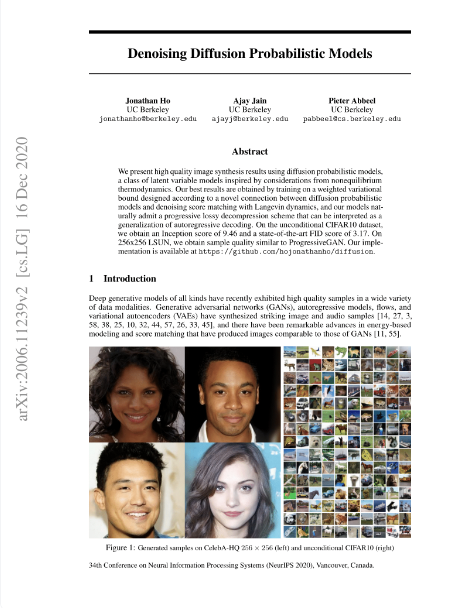
Pre-requisites: Setup and Importing Libraries
- Let’s start with the setup and importing all the required libraries:
from IPython.display import Image
Image(filename='assets/78_annotated-diffusion/ddpm_paper.png')

!pip install -q -U einops datasets matplotlib tqdm

import math
from inspect import isfunction
from functools import partial

%matplotlib inline
import matplotlib.pyplot as plt
from tqdm.auto import tqdm
from einops import rearrange

import torch
from torch import nn, einsum
import torch.nn.functional as F
Helper functions
- Now let’s implement the neural network we have looked at earlier. First we start with a few helper functions.
- Most notably, we define
Residualclass which will add the input to the output of a particular function. That is, it adds a residual connection to a particular function.
def exists(x):
    return x is not None

def default(val, d):
    if exists(val):
        return val
    return d() if isfunction(d) else d

class Residual(nn.Module):
    def __init__(self, fn):
        super().__init__()
        self.fn = fn

    def forward(self, x, *args, **kwargs):
        return self.fn(x, *args, **kwargs) + x

def Upsample(dim):
    return nn.ConvTranspose2d(dim, dim, 4, 2, 1)

def Downsample(dim):
    return nn.Conv2d(dim, dim, 4, 2, 1)
- Note: the parameters of the neural network are shared across time (noise level).
- Thus, for the neural network to keep track of which time step (noise level) it is on, the authors used sinusoidal position embeddings to encode \(t\).
- The
SinusoidalPositionEmbeddingsclass, that we have defined below, takes a tensor of shape(batch_size,1)as input or the noise levels in a batch. - It will then turn this input tensor into a tensor of shape
(batch_size, dim)wheredimis the dimensionality of the position embeddings.
class SinusoidalPositionEmbeddings(nn.Module):
    def __init__(self, dim):
        super().__init__()
        self.dim = dim

    def forward(self, time):
        device = time.device
        half_dim = self.dim // 2
        embeddings = math.log(10000) / (half_dim - 1)
        embeddings = torch.exp(torch.arange(half_dim, device=device) * -embeddings)
        embeddings = time[:, None] * embeddings[None, :]
        embeddings = torch.cat((embeddings.sin(), embeddings.cos()), dim=-1)
        return embeddings
Model Core: ResNet or ConvNeXT
- Now we will look at the meat or the core part of our U-Net model. The original DDPM authors employed a Wide ResNet block via Zagoruyko et al., 2016, however Phil Wang has also introduced support for ConvNeXT block via Liu et al., 2022.
- You are free to choose either or in your final U-Net architecture but both are provided below:
class Block(nn.Module):
    def __init__(self, dim, dim_out, groups = 8):
        super().__init__()
        self.proj = nn.Conv2d(dim, dim_out, 3, padding = 1)
        self.norm = nn.GroupNorm(groups, dim_out)
        self.act = nn.SiLU()

    def forward(self, x, scale_shift = None):
        x = self.proj(x)
        x = self.norm(x)

        if exists(scale_shift):
            scale, shift = scale_shift
            x = x * (scale + 1) + shift

        x = self.act(x)
        return x

class ResnetBlock(nn.Module):
    """https://arxiv.org/abs/1512.03385"""

    def __init__(self, dim, dim_out, *, time_emb_dim=None, groups=8):
        super().__init__()
        self.mlp = (
            nn.Sequential(nn.SiLU(), nn.Linear(time_emb_dim, dim_out))
            if exists(time_emb_dim)
            else None
        )

        self.block1 = Block(dim, dim_out, groups=groups)
        self.block2 = Block(dim_out, dim_out, groups=groups)
        self.res_conv = nn.Conv2d(dim, dim_out, 1) if dim != dim_out else nn.Identity()

    def forward(self, x, time_emb=None):
        h = self.block1(x)

        if exists(self.mlp) and exists(time_emb):
            time_emb = self.mlp(time_emb)
            h = rearrange(time_emb, "b c -> b c 1 1") + h

        h = self.block2(h)
        return h + self.res_conv(x)

class ConvNextBlock(nn.Module):
    """https://arxiv.org/abs/2201.03545"""

    def __init__(self, dim, dim_out, *, time_emb_dim=None, mult=2, norm=True):
        super().__init__()
        self.mlp = (
            nn.Sequential(nn.GELU(), nn.Linear(time_emb_dim, dim))
            if exists(time_emb_dim)
            else None
        )

        self.ds_conv = nn.Conv2d(dim, dim, 7, padding=3, groups=dim)

        self.net = nn.Sequential(
            nn.GroupNorm(1, dim) if norm else nn.Identity(),
            nn.Conv2d(dim, dim_out * mult, 3, padding=1),
            nn.GELU(),
            nn.GroupNorm(1, dim_out * mult),
            nn.Conv2d(dim_out * mult, dim_out, 3, padding=1),
        )

        self.res_conv = nn.Conv2d(dim, dim_out, 1) if dim != dim_out else nn.Identity()

    def forward(self, x, time_emb=None):
        h = self.ds_conv(x)

        if exists(self.mlp) and exists(time_emb):
            condition = self.mlp(time_emb)
            h = h + rearrange(condition, "b c -> b c 1 1")

        h = self.net(h)
        return h + self.res_conv(x)
Attention
- Next, we will look into defining the attention module which was added between the convolutional blocks in DDPM.
- Phil Wang added two variants of attention, a normal multi-headed self-attention from the original Transformer paper (Vaswani et al.,2017), and linear attention variant (Shen et al., 2018).
- Linear attention variant’s time and memory requirements scale linear in the sequence length, as opposed to quadratic for regular attention.
class Attention(nn.Module):
    def __init__(self, dim, heads=4, dim_head=32):
        super().__init__()
        self.scale = dim_head**-0.5
        self.heads = heads
        hidden_dim = dim_head * heads
        self.to_qkv = nn.Conv2d(dim, hidden_dim * 3, 1, bias=False)
        self.to_out = nn.Conv2d(hidden_dim, dim, 1)

    def forward(self, x):
        b, c, h, w = x.shape
        qkv = self.to_qkv(x).chunk(3, dim=1)
        q, k, v = map(
            lambda t: rearrange(t, "b (h c) x y -> b h c (x y)", h=self.heads), qkv
        )
        q = q * self.scale

        sim = einsum("b h d i, b h d j -> b h i j", q, k)
        sim = sim - sim.amax(dim=-1, keepdim=True).detach()
        attn = sim.softmax(dim=-1)

        out = einsum("b h i j, b h d j -> b h i d", attn, v)
        out = rearrange(out, "b h (x y) d -> b (h d) x y", x=h, y=w)
        return self.to_out(out)

class LinearAttention(nn.Module):
    def __init__(self, dim, heads=4, dim_head=32):
        super().__init__()
        self.scale = dim_head**-0.5
        self.heads = heads
        hidden_dim = dim_head * heads
        self.to_qkv = nn.Conv2d(dim, hidden_dim * 3, 1, bias=False)

        self.to_out = nn.Sequential(nn.Conv2d(hidden_dim, dim, 1),
                                    nn.GroupNorm(1, dim))

    def forward(self, x):
        b, c, h, w = x.shape
        qkv = self.to_qkv(x).chunk(3, dim=1)
        q, k, v = map(
            lambda t: rearrange(t, "b (h c) x y -> b h c (x y)", h=self.heads), qkv
        )

        q = q.softmax(dim=-2)
        k = k.softmax(dim=-1)

        q = q * self.scale
        context = torch.einsum("b h d n, b h e n -> b h d e", k, v)

        out = torch.einsum("b h d e, b h d n -> b h e n", context, q)
        out = rearrange(out, "b h c (x y) -> b (h c) x y", h=self.heads, x=h, y=w)
        return self.to_out(out)
- DDPM then adds group normalization to interleave the convolutional/attention layers of the U-Net architecture.
- Below, the
PreNormclass will apply group normalization before the attention layer.- Note, there has been a debate about whether groupnorm is better to be applied before or after attention in Transformers.
class PreNorm(nn.Module):
    def __init__(self, dim, fn):
        super().__init__()
        self.fn = fn
        self.norm = nn.GroupNorm(1, dim)

    def forward(self, x):
        x = self.norm(x)
        return self.fn(x)
Overall network
- Now that we have all the building blocks of the neural network (ResNet/ConvNeXT blocks, attention, positional embeddings, group norm), lets define our entire neural network.
- The task of this neural network is to take in a batch of noisy images and their noise levels and then to output the noise added to the input.
- The network takes a batch of noisy images of shape
(batch_size, num_channels, height, width)and a batch of noise levels of shape(batch_size, 1)as input, and returns a tensor of shape(batch_size, num_channels, height, width). - The network is built up as follows: (source)
- first, a convolutional layer is applied on the batch of noisy images, and position embeddings are computed for the noise levels
- next, a sequence of downsampling stages are applied.
- Each downsampling stage consists of two ResNet/ConvNeXT blocks + groupnorm + attention + residual connection + a downsample operation
- at the middle of the network, again ResNet or ConvNeXT blocks are applied, interleaved with attention
- next, a sequence of upsampling stages are applied.
- Each upsampling stage consists of two ResNet/ConvNeXT blocks + groupnorm + attention + residual connection + an upsample operation
- finally, a ResNet/ConvNeXT block followed by a convolutional layer is applied.
class Unet(nn.Module):
    def __init__(
        self,
        dim,
        init_dim=None,
        out_dim=None,
        dim_mults=(1, 2, 4, 8),
        channels=3,
        with_time_emb=True,
        resnet_block_groups=8,
        use_convnext=True,
        convnext_mult=2,
    ):
        super().__init__()

        # determine dimensions
        self.channels = channels

        init_dim = default(init_dim, dim // 3 * 2)
        self.init_conv = nn.Conv2d(channels, init_dim, 7, padding=3)

        dims = [init_dim, *map(lambda m: dim * m, dim_mults)]
        in_out = list(zip(dims[:-1], dims[1:]))

        if use_convnext:
            block_klass = partial(ConvNextBlock, mult=convnext_mult)
        else:
            block_klass = partial(ResnetBlock, groups=resnet_block_groups)

        # time embeddings
        if with_time_emb:
            time_dim = dim * 4
            self.time_mlp = nn.Sequential(
                SinusoidalPositionEmbeddings(dim),
                nn.Linear(dim, time_dim),
                nn.GELU(),
                nn.Linear(time_dim, time_dim),
            )
        else:
            time_dim = None
            self.time_mlp = None

        # layers
        self.downs = nn.ModuleList([])
        self.ups = nn.ModuleList([])
        num_resolutions = len(in_out)

        for ind, (dim_in, dim_out) in enumerate(in_out):
            is_last = ind >= (num_resolutions - 1)

            self.downs.append(
                nn.ModuleList(
                    [
                        block_klass(dim_in, dim_out, time_emb_dim=time_dim),
                        block_klass(dim_out, dim_out, time_emb_dim=time_dim),
                        Residual(PreNorm(dim_out, LinearAttention(dim_out))),
                        Downsample(dim_out) if not is_last else nn.Identity(),
                    ]
                )
            )

        mid_dim = dims[-1]
        self.mid_block1 = block_klass(mid_dim, mid_dim, time_emb_dim=time_dim)
        self.mid_attn = Residual(PreNorm(mid_dim, Attention(mid_dim)))
        self.mid_block2 = block_klass(mid_dim, mid_dim, time_emb_dim=time_dim)

        for ind, (dim_in, dim_out) in enumerate(reversed(in_out[1:])):
            is_last = ind >= (num_resolutions - 1)

            self.ups.append(
                nn.ModuleList(
                    [
                        block_klass(dim_out * 2, dim_in, time_emb_dim=time_dim),
                        block_klass(dim_in, dim_in, time_emb_dim=time_dim),
                        Residual(PreNorm(dim_in, LinearAttention(dim_in))),
                        Upsample(dim_in) if not is_last else nn.Identity(),
                    ]
                )
            )

        out_dim = default(out_dim, channels)
        self.final_conv = nn.Sequential(
            block_klass(dim, dim), nn.Conv2d(dim, out_dim, 1)
        )

    def forward(self, x, time):
        x = self.init_conv(x)

        t = self.time_mlp(time) if exists(self.time_mlp) else None

        h = []

        # downsample
        for block1, block2, attn, downsample in self.downs:
            x = block1(x, t)
            x = block2(x, t)
            x = attn(x)
            h.append(x)
            x = downsample(x)

        # bottleneck
        x = self.mid_block1(x, t)
        x = self.mid_attn(x)
        x = self.mid_block2(x, t)

        # upsample
        for block1, block2, attn, upsample in self.ups:
            x = torch.cat((x, h.pop()), dim=1)
            x = block1(x, t)
            x = block2(x, t)
            x = attn(x)
            x = upsample(x)

        return self.final_conv(x)
- Note: by default, the noise predictor uses ConvNeXT blocks (as
use_convnextis set to True) and position embeddings are added (aswith_time_embis set to True).
Forward diffusion
- Now lets take a look at the forward diffusion process. Remember forward diffusion process will gradually add noise to an image withing a number of time steps \(T\).
def cosine_beta_schedule(timesteps, s=0.008):
    """
    cosine schedule as proposed in https://arxiv.org/abs/2102.09672
    """
    steps = timesteps + 1
    x = torch.linspace(0, timesteps, steps)
    alphas_cumprod = torch.cos(((x / timesteps) + s) / (1 + s) * torch.pi * 0.5) ** 2
    alphas_cumprod = alphas_cumprod / alphas_cumprod[0]
    betas = 1 - (alphas_cumprod[1:] / alphas_cumprod[:-1])
    return torch.clip(betas, 0.0001, 0.9999)

def linear_beta_schedule(timesteps):
    beta_start = 0.0001
    beta_end = 0.02
    return torch.linspace(beta_start, beta_end, timesteps)

def quadratic_beta_schedule(timesteps):
    beta_start = 0.0001
    beta_end = 0.02
    return torch.linspace(beta_start**0.5, beta_end**0.5, timesteps) ** 2

def sigmoid_beta_schedule(timesteps):
    beta_start = 0.0001
    beta_end = 0.02
    betas = torch.linspace(-6, 6, timesteps)
    return torch.sigmoid(betas) * (beta_end - beta_start) + beta_start
- To start with, let’s use the linear schedule for \(T=200\) time steps and define the various variables from the \(\beta_t\) which we will need, such as the cumulative product of the variances \(\bar{\alpha}_t\)
- Each of the variables below are just 1-dimensional tensors, storing values from \(t\) to \(T\).
- Importantly, we also define an extract function, which will allow us to extract the appropriate \(t\) index for a batch of indices. (source)
timesteps = 200

# define beta schedule
betas = linear_beta_schedule(timesteps=timesteps)

# define alphas
alphas = 1. - betas
alphas_cumprod = torch.cumprod(alphas, axis=0)
alphas_cumprod_prev = F.pad(alphas_cumprod[:-1], (1, 0), value=1.0)
sqrt_recip_alphas = torch.sqrt(1.0 / alphas)

# calculations for diffusion q(x_t \mid\mid x_{t-1}) and others
sqrt_alphas_cumprod = torch.sqrt(alphas_cumprod)
sqrt_one_minus_alphas_cumprod = torch.sqrt(1. - alphas_cumprod)

# calculations for posterior q(x_{t-1} \mid\mid x_t, x_0)
posterior_variance = betas * (1. - alphas_cumprod_prev) / (1. - alphas_cumprod)

def extract(a, t, x_shape):
    batch_size = t.shape[0]
    out = a.gather(-1, t.cpu())
    return out.reshape(batch_size, *((1,) * (len(x_shape) - 1))).to(t.device)
- Now let’s take an image and illustrate how noise is added at each time step of the diffusion process to the PyTorch tensors:
from PIL import Image
import requests

url = 'http://images.cocodataset.org/val2017/000000039769.jpg'
image = Image.open(requests.get(url, stream=True).raw)
image
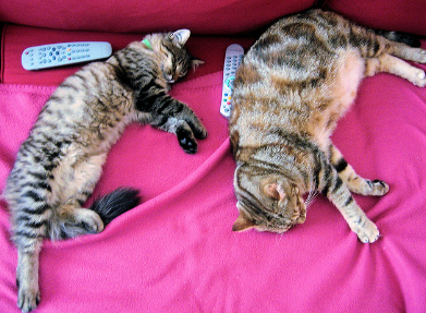
- We first normalize images by dividing by 255 (such that they are in the
[0,1]range), and then make sure they are in the[-1, 1]range.
from torchvision.transforms import Compose, ToTensor, Lambda, ToPILImage, CenterCrop, Resize

image_size = 128
transform = Compose([
    Resize(image_size),
    CenterCrop(image_size),
    ToTensor(), # turn into Numpy array of shape HWC, divide by 255
    Lambda(lambda t: (t * 2) - 1),

])

x_start = transform(image).unsqueeze(0)
x_start.shape
Output:
----------------------------------------------------------------------------------------------------
torch.Size([1, 3, 128, 128])
- We also define the reverse transform, which takes in a PyTorch tensor containing values in
[-1, 1]and turn them back into a PIL image:
import numpy as np

reverse_transform = Compose([
     Lambda(lambda t: (t + 1) / 2),
     Lambda(lambda t: t.permute(1, 2, 0)), # CHW to HWC
     Lambda(lambda t: t * 255.),
     Lambda(lambda t: t.numpy().astype(np.uint8)),
     ToPILImage(),
])
- Let’s run an example and see what it produces:
reverse_transform(x_start.squeeze())

- We can now define the forward diffusion process as in the paper:
# forward diffusion (using the nice property)
def q_sample(x_start, t, noise=None):
    if noise is None:
        noise = torch.randn_like(x_start)

    sqrt_alphas_cumprod_t = extract(sqrt_alphas_cumprod, t, x_start.shape)
    sqrt_one_minus_alphas_cumprod_t = extract(
        sqrt_one_minus_alphas_cumprod, t, x_start.shape
    )

    return sqrt_alphas_cumprod_t * x_start + sqrt_one_minus_alphas_cumprod_t * noise
- Let’s test it on a particular time step and see the image it produces:
def get_noisy_image(x_start, t):
  # add noise
  x_noisy = q_sample(x_start, t=t)

  # turn back into PIL image
  noisy_image = reverse_transform(x_noisy.squeeze())

  return noisy_image
# take time step
t = torch.tensor([40])

get_noisy_image(x_start, t)

- We can see the image is getting more noisy. Now let’s zoom out a bit and visualize this for various time steps:
import matplotlib.pyplot as plt

# use seed for reproducability
torch.manual_seed(0)

# source: https://pytorch.org/vision/stable/auto_examples/plot_transforms.html#sphx-glr-auto-examples-plot-transforms-py
def plot(imgs, with_orig=False, row_title=None, **imshow_kwargs):
    if not isinstance(imgs[0], list):
        # Make a 2d grid even if there's just 1 row
        imgs = [imgs]

    num_rows = len(imgs)
    num_cols = len(imgs[0]) + with_orig
    fig, axs = plt.subplots(figsize=(200,200), nrows=num_rows, ncols=num_cols, squeeze=False)
    for row_idx, row in enumerate(imgs):
        row = [image] + row if with_orig else row
        for col_idx, img in enumerate(row):
            ax = axs[row_idx, col_idx]
            ax.imshow(np.asarray(img), **imshow_kwargs)
            ax.set(xticklabels=[], yticklabels=[], xticks=[], yticks=[])

    if with_orig:
        axs[0, 0].set(title='Original image')
        axs[0, 0].title.set_size(8)
    if row_title is not None:
        for row_idx in range(num_rows):
            axs[row_idx, 0].set(ylabel=row_title[row_idx])

    plt.tight_layout()
plot([get_noisy_image(x_start, torch.tensor([t])) for t in [0, 50, 100, 150, 199]])
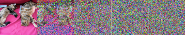
- As we can see above, the image going through forward diffusion is definitely becoming more apparent.
- Thus, we can now move on to defining our loss function. The
denoise_modelwill be our U-Net defined above. We’ll employ the Huber loss between the true and the predicted noise.
def p_losses(denoise_model, x_start, t, noise=None, loss_type="l1"):
    if noise is None:
        noise = torch.randn_like(x_start)

    x_noisy = q_sample(x_start=x_start, t=t, noise=noise)
    predicted_noise = denoise_model(x_noisy, t)

    if loss_type == 'l1':
        loss = F.l1_loss(noise, predicted_noise)
    elif loss_type == 'l2':
        loss = F.mse_loss(noise, predicted_noise)
    elif loss_type == "huber":
        loss = F.smooth_l1_loss(noise, predicted_noise)
    else:
        raise NotImplementedError()

    return loss
Dataset
- Let’s now look into loading up our dataset. A quick note, our dataset needs to make sure all images are resized to the same size.
- Hugging Face’s fashion_mnist dataset which we will use in this example already does that for us with all images having a same resolution of \(28 \times 28\).
from datasets import load_dataset

# load dataset from the hub
dataset = load_dataset("fashion_mnist")
image_size = 28
channels = 1
batch_size = 128
- Now, we will define a function
transformswhich we’ll apply on-the-fly on the entire dataset. - The function just applies some basic image preprocessing: random horizontal flips, rescaling and finally make them have values in the
[-1,1]range.
from torchvision import transforms
from torch.utils.data import DataLoader

# define image transformations (e.g. using torchvision)
transform = Compose([
            transforms.RandomHorizontalFlip(),
            transforms.ToTensor(),
            transforms.Lambda(lambda t: (t * 2) - 1)
])

# define function
def transforms(examples):
   examples["pixel_values"] = [transform(image.convert("L")) for image in examples["image"]]
   del examples["image"]

   return examples

transformed_dataset = dataset.with_transform(transforms).remove_columns("label")

# create dataloader
dataloader = DataLoader(transformed_dataset["train"], batch_size=batch_size, shuffle=True)
batch = next(iter(dataloader))
print(batch.keys())
Output:
----------------------------------------------------------------------------------------------------
dict_keys(['pixel_values'])
Sampling during training
- The paper also talks about sampling from the model during training in order to track progress.
- Ideally, generating new images from a diffusion model happens by reversing the diffusion process:
- We start from \(T\), where we sample pure noise from a Gaussian distribution
- Then use our neural network to gradually de-noise it using the conditional probability it has learned, continuing until we end up at time step \(t\) = 0.
- We can derive a slightly less de-noised image \(x_{(t-1)}\) by plugging in the re-parametrization of the mean, using our noise predictor.
- Remember that the variance is known ahead of time.
- After all of this, ideally, we end up with an image that looks like it came from the real data distribution.
- Lets look at the code for that below:
@torch.no_grad()
def p_sample(model, x, t, t_index):
    betas_t = extract(betas, t, x.shape)
    sqrt_one_minus_alphas_cumprod_t = extract(
        sqrt_one_minus_alphas_cumprod, t, x.shape
    )
    sqrt_recip_alphas_t = extract(sqrt_recip_alphas, t, x.shape)

    # Equation 11 in the paper
    # Use our model (noise predictor) to predict the mean
    model_mean = sqrt_recip_alphas_t * (
        x - betas_t * model(x, t) / sqrt_one_minus_alphas_cumprod_t
    )

    if t_index == 0:
        return model_mean
    else:
        posterior_variance_t = extract(posterior_variance, t, x.shape)
        noise = torch.randn_like(x)
        # Algorithm 2 line 4:
        return model_mean + torch.sqrt(posterior_variance_t) * noise

# Algorithm 2 (including returning all images)
@torch.no_grad()
def p_sample_loop(model, shape):
    device = next(model.parameters()).device

    b = shape[0]
    # start from pure noise (for each example in the batch)
    img = torch.randn(shape, device=device)
    imgs = []

    for i in tqdm(reversed(range(0, timesteps)), desc='sampling loop time step', total=timesteps):
        img = p_sample(model, img, torch.full((b,), i, device=device, dtype=torch.long), i)
        imgs.append(img.cpu().numpy())
    return imgs

@torch.no_grad()
def sample(model, image_size, batch_size=16, channels=3):
    return p_sample_loop(model, shape=(batch_size, channels, image_size, image_size))
- Now, lets get to some training! We will train the model via PyTorch and occasionally save a few image samples using the
samplefunction from above.
from pathlib import Path

def num_to_groups(num, divisor):
    groups = num // divisor
    remainder = num % divisor
    arr = [divisor] * groups
    if remainder > 0:
        arr.append(remainder)
    return arr

results_folder = Path("./results")
results_folder.mkdir(exist_ok = True)
save_and_sample_every = 1000
- Below, we define the model, and move it to the GPU along with defining Adam, a standard optimizer.
from torch.optim import Adam

device = "cuda" if torch.cuda.is_available() else "cpu"

model = Unet(
    dim=image_size,
    channels=channels,
    dim_mults=(1, 2, 4,)
)
model.to(device)

optimizer = Adam(model.parameters(), lr=1e-3)
Training
- Now lets start the training process:
from torchvision.utils import save_image

epochs = 5

for epoch in range(epochs):
    for step, batch in enumerate(dataloader):
      optimizer.zero_grad()

      batch_size = batch["pixel_values"].shape[0]
      batch = batch["pixel_values"].to(device)

      # Algorithm 1 line 3: sample t uniformally for every example in the batch
      t = torch.randint(0, timesteps, (batch_size,), device=device).long()

      loss = p_losses(model, batch, t, loss_type="huber")

      if step % 100 == 0:
        print("Loss:", loss.item())

      loss.backward()
      optimizer.step()

      # save generated images
      if step != 0 and step % save_and_sample_every == 0:
        milestone = step // save_and_sample_every
        batches = num_to_groups(4, batch_size)
        all_images_list = list(map(lambda n: sample(model, batch_size=n, channels=channels), batches))
        all_images = torch.cat(all_images_list, dim=0)
        all_images = (all_images + 1) * 0.5
        save_image(all_images, str(results_folder / f'sample-{milestone}.png'), nrow = 6)
Output:
----------------------------------------------------------------------------------------------------
Loss: 0.46477368474006653
Loss: 0.12143351882696152
Loss: 0.08106148988008499
Loss: 0.0801810547709465
Loss: 0.06122320517897606
Loss: 0.06310459971427917
Loss: 0.05681884288787842
Loss: 0.05729678273200989
Loss: 0.05497899278998375
Loss: 0.04439849033951759
Loss: 0.05415581166744232
Loss: 0.06020551547408104
Loss: 0.046830907464027405
Loss: 0.051029372960329056
Loss: 0.0478244312107563
Loss: 0.046767622232437134
Loss: 0.04305662214756012
Loss: 0.05216279625892639
Loss: 0.04748568311333656
Loss: 0.05107741802930832
Loss: 0.04588869959115982
Loss: 0.043014321476221085
Loss: 0.046371955424547195
Loss: 0.04952816292643547
Loss: 0.04472338408231735
- And finally, let’s look at our inference or sampling from the
samplefunction we defined above.
# sample 64 images
samples = sample(model, image_size=image_size, batch_size=64, channels=channels)

# show a random one
random_index = 5
plt.imshow(samples[-1][random_index].reshape(image_size, image_size, channels), cmap="gray")
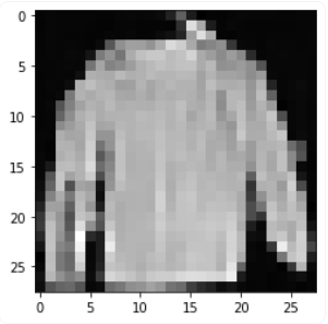
- Seems like the model is capable of generating a nice T-shirt! Keep in mind that the dataset we trained on is pretty low-resolution (28x28).
Creating a GIF
- Lastly, in order to see the progression of the de-noising process, we can create a GIF:
import matplotlib.animation as animation

random_index = 53

fig = plt.figure()
ims = []
for i in range(timesteps):
    im = plt.imshow(samples[i][random_index].reshape(image_size, image_size, channels), cmap="gray", animated=True)
    ims.append([im])

animate = animation.ArtistAnimation(fig, ims, interval=50, blit=True, repeat_delay=1000)
animate.save('diffusion.gif')
plt.show()

- Hopefully this was beneficial in clarifying the diffusion model concepts!
- Furthermore, it his highly recommend looking at Hugging Face’s Training with Diffusers notebook to see how to leverage their Diffusion library to train a simple model.
- And, for inference, they also provide this notebook where you can see the images being generated.
denoising-diffusion-pytorch package
- While Diffusion models have not yet been democratized to the same degree as other older architectures/approaches in Machine Learning, there are still implementations available for use. The easiest way to use a diffusion model in PyTorch is to use the
denoising-diffusion-pytorchpackage, which implements an image diffusion model like the one discussed in this article. To install the package, simply type the following command in the terminal:
pip install denoising_diffusion_pytorch
Minimal Example
- To train a model and generate images, we first import the necessary packages:
import torch
from denoising_diffusion_pytorch import Unet, GaussianDiffusion
- Next, we define our network architecture, in this case a U-Net. The
dimparameter specifies the number of feature maps before the first down-sampling, and thedim_multsparameter provides multiplicands for this value and successive down-samplings:
model = Unet(
    dim = 64,
    dim_mults = (1, 2, 4, 8)
)
- Now that our network architecture is defined, we need to define the diffusion model itself. We pass in the U-Net model that we just defined along with several parameters - the size of images to generate, the number of timesteps in the diffusion process, and a choice between the L1 and L2 norms.
diffusion = GaussianDiffusion(
    model,
    image_size = 128,
    timesteps = 1000,   # number of steps
    loss_type = 'l1'    # L1 or L2
)
- Now that the diffusion model is defined, it’s time to train. We generate random data to train on, and then train the diffusion model in the usual fashion:
training_images = torch.randn(8, 3, 128, 128)
loss = diffusion(training_images)
loss.backward()
- Once the model is trained, we can finally generate images by using the
sample()method of thediffusionobject. Here we generate 4 images, which are only noise given that our training data was random:
sampled_images = diffusion.sample(batch_size = 4)
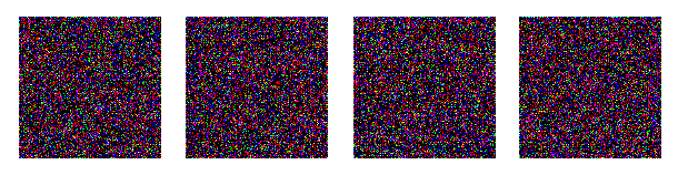
Training on Custom Data
- The
denoising-diffusion-pytorchpackage also allow you to train a diffusion model on a specific dataset. Simply replace the'path/to/your/images'string with the dataset directory path in theTrainer()object below, and changeimage_sizeto the appropriate value. After that, simply run the code to train the model, and then sample as before. Note that PyTorch must be compiled with CUDA enabled in order to use theTrainerclass:
from denoising_diffusion_pytorch import Unet, GaussianDiffusion, Trainer

model = Unet(
    dim = 64,
    dim_mults = (1, 2, 4, 8)
).cuda()

diffusion = GaussianDiffusion(
    model,
    image_size = 128,
    timesteps = 1000,   # number of steps
    loss_type = 'l1'    # L1 or L2
).cuda()

trainer = Trainer(
    diffusion,
    'path/to/your/images',
    train_batch_size = 32,
    train_lr = 2e-5,
    train_num_steps = 700000,         # total training steps
    gradient_accumulate_every = 2,    # gradient accumulation steps
    ema_decay = 0.995,                # exponential moving average decay
    amp = True                        # turn on mixed precision
)

trainer.train()
- Below you can see progressive denoising from multivariate Gaussian noise to MNIST digits akin to reverse diffusion:
HuggingFace Diffusers
- HuggingFace diffusers provides pretrained diffusion models across multiple modalities, such as vision and audio, and serves as a modular toolbox for inference and training of diffusion models.

- More precisely, HuggingFace Diffusers offers:
- State-of-the-art diffusion pipelines that can be run in inference with just a couple of lines of code.
- Various noise schedulers that can be used interchangeably for the prefered speed vs. quality trade-off in inference.
- Multiple types of models, such as UNet, that can be used as building blocks in an end-to-end diffusion system.
- Training examples to show how to train the most popular diffusion models.
Implementations
Stable Diffusion
- Stable Diffusion (blog) is a state of the art text-to-image model that generates images from text. It’s makes it’s high performance models available to the public at large to use here.
- Stable Diffusion is a text-to-image latent diffusion model created by the researchers and engineers from CompVis, Stability AI and LAION. It is trained on 512x512 images from a subset of the LAION-5B database which is the largest, freely accessible multi-modal dataset.
- Let’s now look at how it works with the illustrations below by Jay Alammar.
- Stable Diffusion is quite versatile because it can be used in a variety of ways.
- In the image we see above, we can see that it can take text as input and output a generated image. This is the primary use case, however, it is not the only one.
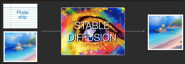
- As we can see from the image above, another use case of Stable Diffusion is with image and text as input, and it will output a generated image again. This is called img2img.
- It’s able to be so versatile because Stable Diffusion is not one monolith model, but a system made up of several components and models.
- To be specific, Stable Diffusion is made up of a:
- 1) Text Understanding component
- 2) Image Generation component
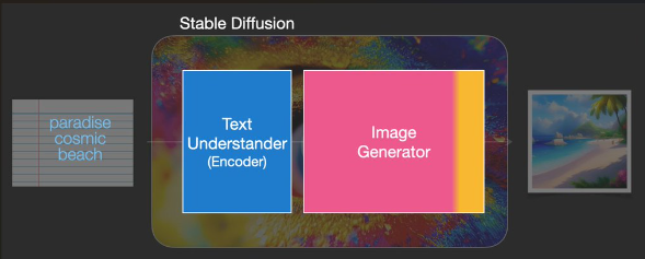
- The text understanding component is actually the text encoder used within CLIP.
- As we can see represented in the image below, Stable Diffusion takes the input text within the Text Understander component and returns a vector representing each token in the text.
- This information is then passed over to the Image Generator component which internally is composed of 2 components as well.
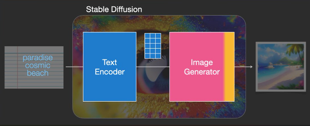
- Now, referring to the image below, let’s look at the two components within the Image Generator component.
- Image Information Creator:
- This is the ‘secret sauce’ of Stable Diffusion as it runs for a number of steps refining the information that should go in the image that will become the model’s output.
- Image Decoder:
- This component takes the processed information and paints the picture.
- Image Information Creator:
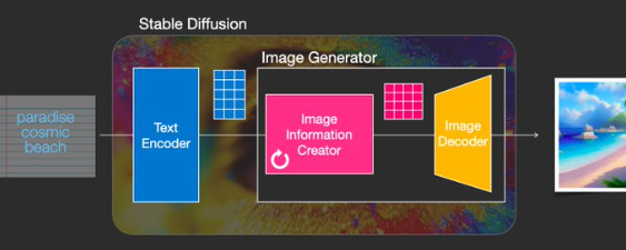
- Let’s zoom out for a second and look at the higher level components we have so far all working together for the image generation task:
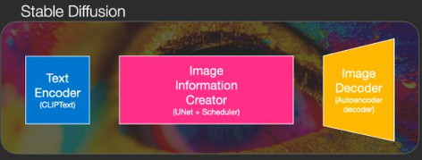
- All the 3 components above are actually individual neural networks working together, specifically, they are:
- CLIPText: Used to encode the text
- U-Net + scheduler: Used to gradually process image information(latent diffusion)
- Autoencoder Decoder: paints the final image
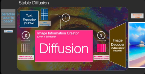
-
Above we can see the steps that Stable Diffusion takes to generate its images.
-
Lastly, let’s zoom into the image decoder and get a better understanding of its inner workings. Remember the image decoder is one of the two components the image generator comprises of
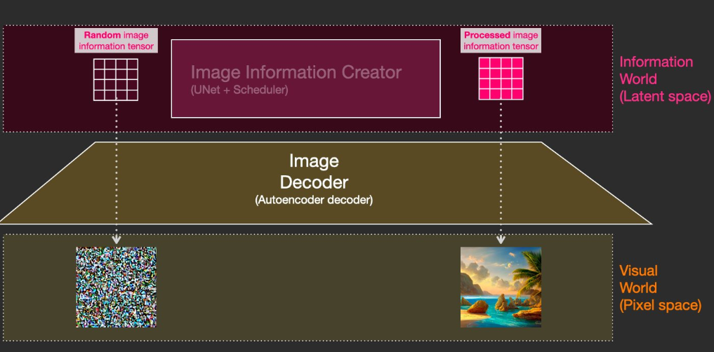
- The random vector is considered to be random noise.
- Stable Diffusion is able to obtain it’s speed from the fact that the processing happens in the latent space (which needs less calculations as compared to the pixel space).
Dream Studio
- Dream Studio is Stable Diffusion’s AI Art Web App Tool.
- DreamStudio is a new suite of generative media tools engineered to grant everyone the power of limitless imagination and the effortless ease of visual expression through a combination of natural language processing and revolutionary input controls for accelerated creativity.
Midjourney
- Midjourney is an independent research lab exploring new mediums of thought and expanding the imaginative powers of the human species.
- Midjourney has not made it’s architecture details publicly available, but one has to think they still leverage diffusion models in some fashion.
- While Dall-E 2 creates more realistic images, MidJourney shines in adapting real art styles into creating an image of any combination of things your heart desires.
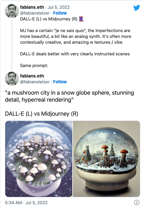
DALL-E 2
- DALL-E 2 utilized diffusion models to create its images and was created by OpenAI.
- DALL-E 2 can make realistic edits to existing images from a natural language caption.
- It can add and remove elements while taking shadows, reflections, and textures into consideration.
- DALL-E 2 has learned the relationship between images and the text used to describe them.
- It uses diffusion, which starts with a pattern of random dots and gradually alters that pattern towards an image when it recognizes specific aspects of that image.
- OpenAI has limited the ability for DALL-E 2 to generate violent, hate, or adult images.
- By removing the most explicit content from the training data, OpenAI has minimized DALL-E 2’s exposure to these concepts.
- They have also used advanced techniques to prevent photorealistic generations of real individuals’ faces, including those of public figures.
- Among the most important building blocks in the DALL-E 2 architecture is CLIP to function as the main bridge between text and images.
Related: CLIP (Contrastive Language-Image Pre-Training)
- While CLIP does not use a diffusion model, it is essential to understand DALL-E 2 so let’s do a quick recap of CLIP’s architecture.
- CLIP is a neural network trained on a variety of (image, text) pairs.
- It can be instructed in natural language to predict the most relevant text snippet, given an image, without directly optimizing for the task, similarly to the zero-shot capabilities of GPT-2 and 3.
- CLIP is a multi-modal vision and language model.
- It can be used for image-text similarity and for zero-shot image classification.
- CLIP uses a ViT like transformer to get visual features and a causal language model to get the text features.
- Both the text and visual features are then projected to a latent space with identical dimension. The dot product between the projected image and text features is then used as a similar score.
- CLIP enables us to take textual phrases and understand how they map onto images
Gallery
- Showcasing a few images generated via Diffusion Models along with their text prompts given:
- A Corgi puppy painted like the Mona Lisa:
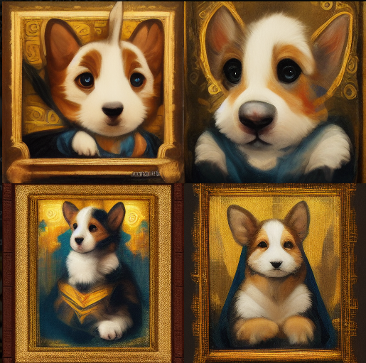
- Beyonce sitting at a desk and coding:
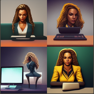
- Snow in Hawaii:
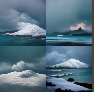
- Sun coming in from a big window with curtains and casting a shadow on the rest of the room, artistic style:
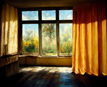
- The Taj Mahal painted in Starry Night by Vincent Van Gogh:
FAQs
At a high level, how do diffusion models work? What are some other models that are useful for image generation, and how do they compare to diffusion models?
High-Level Overview of Diffusion Models
- Diffusion models are a type of generative model that creates data by gradually denoising a sample from a noise distribution. The process involves two main phases: a forward diffusion process that corrupts the data by adding noise, and a reverse denoising process that learns to remove the noise step-by-step to recover the original data. Here’s a high-level breakdown:
Forward Diffusion Process
- Start with a Data Sample: Begin with a real data sample, such as an image.
- Add Noise Incrementally: Over a series of steps \(t\), progressively add Gaussian noise to the sample. The amount of noise added at each step is controlled by a noise schedule \(\beta_t\). \(x_t = \sqrt{\alpha_t} x_{t-1} + \sqrt{1 - \alpha_t} \epsilon, \quad \epsilon \sim N(0, I)\)
- Result in Noisy Data: By the final step, the data is almost completely transformed into pure noise.
Reverse Denoising Process
- Start with Noise: Begin with a sample of pure noise.
- Learn to Remove Noise: A neural network is trained to predict and remove the added noise at each step, effectively denoising the sample. \(p_\theta(x_{t-1} \mid\mid x_t) = N(x_{t-1}; \mu_\theta(x_t, t), \Sigma_\theta(x_t, t))\)
- Recover Original Data: Iteratively apply the denoising steps to transform the noise back into a data sample that resembles the original data distribution.
Other Models for Image Generation
- Several other models are commonly used for image generation, each with unique characteristics and methodologies. Here are some notable ones:
Generative Adversarial Networks (GANs)
- How They Work:
- Two Networks: Consist of a generator and a discriminator network that compete against each other.
- Generator: Creates fake images from random noise.
- Discriminator: Tries to distinguish between real images and fake images produced by the generator.
-
Adversarial Training: The generator improves to produce more realistic images as the discriminator gets better at distinguishing them.
- Comparison to Diffusion Models:
- Training Stability: GANs can be harder to train and may suffer from issues like mode collapse.
- Speed: Typically faster in generation since GANs do not require iterative denoising steps.
- Quality: Can produce high-quality images, but may lack diversity in the generated samples compared to diffusion models.
Variational Autoencoders (VAEs)
- How They Work:
- Encoder-Decoder Architecture: Consist of an encoder that maps input data to a latent space and a decoder that reconstructs the data from the latent space.
- Latent Space Sampling: Imposes a probabilistic structure on the latent space, encouraging smooth transitions and interpolation.
-
Variational Inference: Uses a loss function that includes a reconstruction term and a regularization term (Kullback-Leibler divergence).
- Comparison to Diffusion Models:
- Latent Space Representation: VAEs provide an explicit latent space representation, which can be useful for tasks like interpolation and manipulation.
- Sample Quality: VAEs typically produce lower-quality images compared to GANs and diffusion models.
- Training Stability: Generally more stable and easier to train than GANs.
Autoregressive Models
- How They Work:
- Sequential Generation: Generate images pixel-by-pixel or patch-by-patch in a sequential manner.
- Conditional Dependencies: Each pixel or patch is conditioned on the previously generated ones.
-
Examples: PixelRNN, PixelCNN.
- Comparison to Diffusion Models:
- Generation Time: Autoregressive models can be slow due to sequential nature.
- Quality: Can produce high-quality images with strong dependencies between pixels.
- Flexibility: Can naturally model complex dependencies but are computationally intensive.
Flow-based Models
- How They Work:
- Invertible Transformations: Use a series of invertible transformations to map data to a latent space and vice versa.
- Exact Likelihood: Allow exact computation of the data likelihood, making them powerful for density estimation.
- Examples: RealNVP, Glow.
- Comparison to Diffusion Models:
- Efficiency: Flow-based models can be efficient in both training and sampling due to invertible nature.
- Quality: Produce high-quality images but may require more complex architectures for challenging datasets.
- Interpretability: Provide explicit likelihood estimates and interpretable latent spaces.
Summary
- Diffusion Models: Offer a robust and principled approach to image generation with a focus on iterative denoising. They provide high-quality samples but can be slower due to the iterative nature.
- GANs: Known for producing very high-quality images quickly but can be challenging to train due to adversarial dynamics.
- VAEs: Provide stable training and useful latent space representations, though often at the cost of sample quality.
- Autoregressive Models: Capable of modeling complex dependencies with high-quality outputs, but slow due to sequential generation.
- Flow-based Models: Efficient and interpretable with exact likelihood estimation, balancing quality and computational requirements.
- In summary, each model type has its strengths and weaknesses, making them suitable for different applications and preferences in the trade-off between quality, efficiency, and ease of training.
What is the difference between DDPM and DDIMs models?
- Denoising Diffusion Probabilistic Models (DDPM) and Denoising Diffusion Implicit Models (DDIMs) are both types of diffusion models used for generative tasks, but they differ in their approach to the reverse diffusion process, which leads to differences in their efficiency and the quality of generated samples. Here’s a detailed explanation of both models and their differences:
DDPM
- DDPMs are a class of generative models that create data by reversing a Markovian diffusion process. The diffusion process gradually adds noise to the data in several steps until it becomes nearly pure Gaussian noise. The model then learns to reverse this process, step by step, to generate new data samples.
Key Characteristics
- Forward Process:
- The forward diffusion process adds Gaussian noise to data over \(T\) timesteps.
- Each step is defined as: \(q(x_t \mid\mid x_{t-1}) = N(x_t; \sqrt{1 - \beta_t} x_{t-1}, \beta_t I)\)
- \(\beta_t\) is the noise schedule, typically increasing linearly or following another schedule over time.
- Reverse Process:
- The reverse process is learned using a neural network to approximate the conditional probabilities: \(p_\theta(x_{t-1} \mid\mid x_t) = N(x_{t-1}; \mu_\theta(x_t, t), \Sigma_\theta(x_t, t))\)
- The mean \(\mu_\theta\) and variance \(\Sigma_\theta\) are predicted by the neural network.
- Training:
- The model is trained to minimize the variational bound on the data likelihood, which involves matching the reverse process to the true posterior of the forward process.
- Sampling:
- Sampling involves running the reverse process starting from Gaussian noise \(x_T\), iteratively refining it to produce a sample \(x_0\).
Advantages and Disadvantages
- Advantages:
- Generates high-quality samples.
- Well-grounded in probabilistic principles, leading to stable training.
- Disadvantages:
- The reverse process is slow because it involves many iterative steps.
- Each step requires a neural network forward pass, making the sampling process computationally expensive.
DDIMs
- DDIMss are a variation of diffusion models that introduce a non-Markovian forward process, which allows for a more efficient reverse process. The key idea is to find a deterministic mapping that approximates the same data distribution as the original Markovian process used in DDPMs.
Key Characteristics
- Forward Process:
- The forward process in DDIMss can be viewed as a non-Markovian process that achieves the same goal of perturbing data into noise.
- Instead of a strict Markov chain, DDIMss introduce a sequence of latent variables that allow skipping steps while preserving the ability to reverse the process.
- Reverse Process:
- The reverse process becomes deterministic, significantly speeding up the sampling process.
- The reverse step is defined by a deterministic mapping, approximating the reverse diffusion without needing as many steps as DDPMs.
- This is achieved through a reparameterization that relates the noise-added data at different timesteps directly.
- Training:
- Training is similar to DDPMs but leverages the deterministic nature of the reverse process for improved efficiency.
- Sampling:
- Sampling in DDIMss can be done with fewer steps while still producing high-quality samples.
- The deterministic reverse process can potentially offer more control over the generation process, enabling finer adjustments to the generated data.
Advantages and Disadvantages
- Advantages:
- Faster sampling compared to DDPMs due to the deterministic reverse process.
- Fewer sampling steps needed while maintaining or even improving sample quality.
- Disadvantages:
- The theoretical underpinnings are less straightforward compared to the probabilistic foundations of DDPMs.
- Potentially less flexibility in certain applications where stochasticity in the reverse process is beneficial.
Key Differences
- Process Type:
- DDPM: Markovian forward process with a stochastic reverse process.
- DDIMs: Non-Markovian forward process with a deterministic reverse process.
- Sampling Efficiency:
- DDPM: Requires many reverse steps, making it computationally expensive.
- DDIMs: Achieves faster sampling with fewer steps.
- Reverse Process:
- DDPM: Stochastic reverse process, which involves sampling from a learned Gaussian distribution at each step.
- DDIMs: Deterministic reverse process, which directly maps noisy data to clean data without stochastic sampling.
- Complexity and Flexibility:
- DDPM: More flexible in representing complex distributions due to the stochastic nature of the reverse process.
- DDIMs: More efficient and potentially more controllable but may be less flexible in certain scenarios.
- In summary, while both DDPM and DDIMs are powerful diffusion-based generative models, DDIMss offer a more efficient sampling process by employing a deterministic reverse process, leading to faster generation of samples without compromising quality. DDPMs, on the other hand, are grounded in a robust probabilistic framework, making them more flexible but slower in practice.
In diffusion models, there is a forward diffusion process and a reverse diffusion/denoising process. When do you use which during training and inference?
- In diffusion models, which are a class of generative models, the forward diffusion process and the denoising process play distinct roles during training and inference. Understanding when and how these processes are used is key to grasping how diffusion models work.
- Forward Diffusion Process
- During Training:
- Noise Addition: In the forward diffusion process, noise is gradually added to the data over several steps or iterations. This process transforms the original data into a pure noise distribution through a predefined sequence of steps.
- Training Objective: The model is trained to predict the noise that was added at each step. Essentially, it learns to reverse the diffusion process.
- During Inference:
- Not Directly Used: The forward diffusion process is not explicitly used during inference. However, the knowledge gained during training (about how noise is added) is implicitly used to guide the denoising process.
- During Training:
- Denoising Process
- During Training:
- Learning to Reverse Noise: The model learns to denoise the data, i.e., to reverse the forward diffusion process. It does this by predicting the noise that was added at each step during the forward diffusion and then subtracting this noise.
- Parameter Optimization: The parameters of the model are optimized to make accurate predictions of the added noise, thereby learning to gradually denoise the data back to its original form.
- During Inference:
- Data Generation: The denoising process is the key to generating new data. Starting from pure noise, the model iteratively denoises this input, using the reverse of the forward process, to generate a sample.
- Iterative Refinement: At each step, the model predicts the noise to remove, effectively refining the sample from random noise into a coherent output.
- During Training:
- Summary
- Training Phase: Both the forward diffusion (adding noise) and the denoising (removing noise) processes are actively used. The model learns how to reverse the gradual corruption of the data (caused by adding noise) by being trained to predict and remove the noise at each step.
- Inference Phase: Only the denoising process is used, where the model starts with noise and iteratively applies the learned denoising steps to generate a sample. The forward process is not explicitly run during inference, but its principles underpin the reverse process.
- Forward Diffusion Process
- In essence, the forward diffusion process is crucial for training the model to understand and reverse the noise addition, while the denoising process is used both in training (to learn this reversal) and in inference (to generate new data).
What are the loss functions used in Diffusion Models?
-
Diffusion models are trained using a small family of closely related loss functions that all arise from the same underlying objective: likelihood maximization under a diffusion process. What often appears to be a diverse set of training criteria—ELBO formulations, noise-prediction MSE, score matching, or alternative parameterizations—is best understood as different expressions of a single probabilistic principle rather than fundamentally different goals.
-
All major diffusion training losses originate from maximizing a variational bound on the data likelihood (the ELBO). Because the forward diffusion process is Gaussian, the KL divergence terms that appear in this bound simplify into tractable regression objectives. The remaining differences across methods come from how the model is parameterized: it may be trained to predict added noise, the original data, a velocity-like combination, or the score function, but these are mathematically interchangeable views of the same optimization problem.
-
From this perspective, the widely used mean-squared-error loss for noise prediction is not a heuristic or approximation to likelihood training. It is likelihood training—rewritten in the simplest, most numerically stable form enabled by the Gaussian structure of diffusion processes.
Variational ELBO loss (foundational objective)
-
The original formulation of diffusion models appears in Deep Unsupervised Learning using Nonequilibrium Thermodynamics by Sohl-Dickstein et al. (2015) and was made practical in Denoising Diffusion Probabilistic Models by Ho et al. (2020).
-
Diffusion models introduce latent variables \(x_1, \dots, x_T\) and optimize a variational lower bound (ELBO) on the data likelihood:
- This ELBO decomposes into KL divergences between the true reverse diffusion process and the learned reverse process, plus a reconstruction term. Conceptually, this is the most principled training objective, but it is cumbersome to compute directly.
Noise-prediction MSE loss (standard in practice)
-
Ho et al. show in Denoising Diffusion Probabilistic Models by Ho et al. (2020) that the ELBO simplifies dramatically when both forward and reverse transitions are Gaussian.
-
Using the forward reparameterization:
- the KL terms reduce to squared error between true noise \(\varepsilon\) and predicted noise \(\varepsilon_\theta(x_t,t)\):
- This regression loss is a simplified, reparameterized form of the ELBO with constants and timestep-dependent weights removed. It is the dominant loss used in modern systems such as High-Resolution Image Synthesis with Latent Diffusion Models by Rombach et al. (2022), Photorealistic Text-to-Image Diffusion Models with Deep Language Understanding by Saharia et al. (2022), and Hierarchical Text-Conditional Image Generation with CLIP Latents by Ramesh et al. (2022).
\(x_0\)-prediction loss
- Instead of predicting noise, the model can directly predict the clean sample:
- This parameterization is mathematically equivalent to noise prediction, differing only by a linear transformation. It is discussed in Denoising Diffusion Probabilistic Models by Ho et al. (2020) and used in various follow-up works.
v-prediction (velocity) loss
- Introduced and popularized in Progressive Distillation for Fast Sampling of Diffusion Models by Salimans and Ho (2022) and used extensively in large-scale systems, the model predicts:
- with loss:
- This formulation improves numerical stability and balances learning across noise levels.
Score-matching loss (continuous-time diffusion)
-
Score-based diffusion models were introduced in Generative Modeling by Estimating Gradients of the Data Distribution by Song and Ermon (2019) and unified with SDEs in Score-Based Generative Modeling through Stochastic Differential Equations by Song et al. (2021).
-
Here, the model learns the score function \(s_\theta(x_t,t) \approx \nabla_x \log p_t(x_t)\) via denoising score matching:
- This is the continuous-time analogue of the discrete MSE noise-prediction objective and is equivalent to ELBO optimization under an SDE formulation.
Weighted, perceptual, and hybrid losses
-
Some systems incorporate:
- timestep-weighted MSE,
- perceptual losses in feature space,
- or auxiliary adversarial objectives.
-
These appear in works such as Diffusion Models Beat GANs on Image Synthesis by Dhariwal and Nichol (2021) and are extensions rather than replacements of the core diffusion loss.
If diffusion models are trained by maximizing a variational lower bound (ELBO) on the data log-likelihood, how does this probabilistic objective reconcile with the simple regression-style MSE loss used for noise prediction in practice?
-
The mean squared error (MSE) noise-prediction loss commonly used in diffusion models is not merely a heuristic substitute for likelihood training. Rather, it is a principled, reparameterized, and simplified formulation of the variational lower bound (ELBO) on the data log-likelihood. This regression-style loss is fully consistent with ELBO-based likelihood objectives and arises naturally from the structure of the diffusion framework.
-
Specifically, due to the Gaussian nature of the forward diffusion process and the use of a noise-based parameterization, the MSE loss can be derived directly from the ELBO formulation. The simplification is exact up to constant factors and known weighting terms, preserving the theoretical integrity of likelihood-based training while enabling efficient and effective learning in practice.
-
Starting from the ELBO:
- Denoising Diffusion Probabilistic Models (DDPMs) introduce a sequence of latent variables \(x_1, \dots, x_T\) with the same dimensionality as the data \(x_0\). The marginal data likelihood is written using these latent variables as
-
This expression is the evidence lower bound (ELBO). Because both the forward process \(q\) and the reverse process \(p_\theta\) are Markovian, the ELBO can be decomposed into a sum of interpretable terms.
-
Specifically, it consists of:
- a reconstruction term at timestep \(t = 0\),
- a sum of Kullback–Leibler divergences between the true reverse posterior and the learned reverse transitions,
- a prior-matching term at the final timestep \(T\).
-
Writing this decomposition explicitly yields
\[\mathrm{ELBO} =-\sum_{t=2}^T \mathrm{KL}\big( q(x_{t-1} \mid x_t, x_0) \Vert p_\theta(x_{t-1} \mid x_t) \big) -\mathrm{KL}\big( q(x_T \mid x_0) \Vert p(x_T) \big) +\log p_\theta(x_0 \mid x_1)\]- Maximizing the ELBO corresponds to minimizing each of these KL divergence terms while ensuring accurate reconstruction at the final denoising step.
-
Gaussian structure collapses the KL terms:
-
A key design choice in diffusion models is that both the forward diffusion process and the learned reverse process are Gaussian.
-
Concretely:
- the forward process \(q(x_t \mid x_{t-1})\) is a fixed Gaussian with known variance,
- the posterior \(q(x_{t-1} \mid x_t, x_0)\) has a closed-form Gaussian expression,
- the reverse model \(p_\theta(x_{t-1} \mid x_t)\) is parameterized as a Gaussian whose mean is predicted by a neural network, with variance either fixed or learned.
-
For two Gaussians with identical covariance matrices, the KL divergence reduces to a squared error between their means, up to a known constant. As a result, each KL term in the ELBO becomes a weighted quadratic loss between the true reverse mean and the model’s predicted mean.
-
Thus, ELBO maximization already reduces to a regression problem under these Gaussian assumptions.
-
-
Reparameterizing the reverse mean via noise:
-
Instead of predicting the reverse mean directly, Denoising Diffusion Probabilistic Models by Ho et al. (2020) introduce a reparameterization based on the injected noise.
-
The forward process admits the closed-form representation:
\[x_t =\sqrt{\bar{\alpha}_t}, x_0 +\sqrt{1 - \bar{\alpha}_t}, \varepsilon, \quad \varepsilon \sim \mathcal{N}(0, I)\]- where \(\bar{\alpha}_t\) is the cumulative product of noise schedule coefficients.
-
Under this parameterization, predicting:
- the reverse-process mean,
- the clean data \(x_0\),
-
or the noise \(\varepsilon\)
- … are all mathematically equivalent, differing only by known linear transformations.
-
When the Gaussian KL term is rewritten using this noise parameterization, each KL divergence becomes proportional to:
\[\mathbb{E} \left[ |\varepsilon - \varepsilon_\theta(x_t, t)|^2 \right]\]- where \(\varepsilon_\theta\) is the neural network’s prediction of the injected noise. The proportionality constant depends only on the timestep \(t\) and the noise schedule, not on the model parameters \(\theta\).
-
-
Dropping constants and timestep-dependent weights:
-
The full ELBO contains several components that do not affect the location of the optimum:
- additive constants independent of \(\theta\),
- timestep-dependent scaling factors multiplying each squared error,
- a reconstruction term \(\log p_\theta(x_0 \mid x_1)\) that is often small or noisy.
-
Ho et al. empirically observe that removing these terms yields a simpler objective with improved optimization behavior, while preserving the same optimal parameters.
-
This leads to the simplified training loss
\[\mathbb{E}_{x_0, \varepsilon, t} \left[ |\varepsilon - \varepsilon_\theta(x_t, t)|^2 \right]\] -
This loss is therefore not a different objective, but the ELBO with:
- constants removed,
- timestep weights ignored or absorbed,
- a specific and convenient parameterization choice.
-
-
Continuous-time and score-based interpretation:
-
In continuous-time diffusion models, the discrete ELBO converges to an integral objective over time. In this limit, the same training objective can be interpreted as:
- denoising score matching,
- minimizing the Fisher divergence between the true score field \(\nabla_x \log p_t(x)\) and the learned score.
-
Thus, even in score-based and SDE formulations, the regression-style loss remains a likelihood-based objective, expressed in score space rather than density space.
-
What is the Denoising Score Matching Loss in Diffusion models? Explain with an equation and intuition.
- The Denoising Score Matching Loss is a critical component in the training of diffusion models, a class of generative models. This loss function is designed to train the model to effectively reverse a diffusion process, which gradually adds noise to the data over a series of steps.
- Denoising Score Matching Loss: Equation and Intuition
- Background:
- In diffusion models, the data is incrementally noised over a sequence of steps. The reverse process, which the model learns, involves denoising or reversing this noise addition to recreate the original data from noise.
- Equation:
-
The denoising score matching loss at a particular timestep \(t\) can be formulated as:
\[L(\theta)=\mathbb{E}_{x_0, \epsilon \sim N(0, I), t}\left[\left\lVert s_\theta\left(x_t, t\right)-\nabla_{x_t} \log p_{t \mid 0}\left(x_t \mid x_0\right)\right\rVert^2\right]\]- where, \(x_0\) is the original data, \(x_t\) is the noised data at timestep \(t\), and \(\epsilon\) is the added Gaussian noise.
- \(s_\theta\left(x_t, t\right)\) is the score (gradient of the log probability) predicted by the model with parameters \(\theta\).
- \(\nabla_{x_t} \log p_{t \mid 0}\left(x_t \mid x_0\right)\) is the true score, which is the gradient of the log probability of the noised data \(x_t\) conditioned on the original data \(x_0\).
- Intuition:
- The loss function encourages the model to predict the gradient of the log probability of the noised data with respect to the data itself. Essentially, it’s training the model to estimate how to reverse the diffusion process at each step.
- By minimizing this loss, the model learns to approximate the reverse of the noising process, thereby learning to generate data starting from noise.
- This process effectively teaches the model the denoising direction at each step of the noised data, guiding it on how to gradually remove noise and reconstruct the original data.
- Importance in Training: The denoising score matching loss is crucial for training diffusion models to generate high-quality samples. It ensures that the model learns a detailed and accurate reverse mapping of the diffusion process, capturing the complex data distribution.
- Advantages: This approach allows diffusion models to generate samples that are often of higher quality and more diverse compared to other generative models, as it carefully guides the generative process through the learned noise reversal.
- Background:
- In summary, the denoising score matching loss in diffusion models is fundamental in training these models to effectively reverse the process of gradual noise addition, enabling the generation of high-quality data samples from a noise distribution. This loss function is key to the model’s ability to learn the intricate details of the data distribution and the precise dynamics of the denoising process.
What does the “stable” in stable diffusion refer to?
- The “stability” in stable diffusion also refers to maintaining image content in the latent space throughout the diffusion process. In diffusion models, the image is transformed from the pixel space to the “latent space” – this is a high-dimensional abstract representation of the image. Here are the differences between the two:
- Pixel Space:
- This refers to the space in which the data (such as images) is represented in its raw form – as pixels.
- Each dimension corresponds to a pixel value, so an image of size 100x100 would have a pixel space of 10,000 dimensions.
- Pixel space representations are direct and intuitive but can be very high-dimensional and sparse for complex data like images.
- Latent Space:
- Latent space is a lower-dimensional space where data is represented in a more compressed and abstract form.
- Generative models, like Variational Autoencoders (VAEs) or Generative Adversarial Networks (GANs), encode high-dimensional data (from pixel space) into this lower-dimensional latent space.
- The latent representation captures the essential features or characteristics of the data, allowing for more efficient processing and manipulation.
- Operations and transformations are often performed in latent space because they can be more meaningful and computationally efficient. For example, interpolating between two points in latent space can result in a smooth transition between two images when decoded back to pixel space.
- Pixel Space:
- The “Stable” in Stable Diffusion refers to the fact that the forward and reverse diffusion process occur in a low-dimensional latent space vs. a high-dimensional pixel space leading to stability during diffusion. If the latent space becomes unstable and loses image content too quickly, the generated pixel space images will be poor.
- Stable diffusion uses techniques to keep the latent space more stable throughout the diffusion process:
- The denoising model tries to remove noise while preserving latent space content at each step.
- Regularization prevents the denoising model from changing too drastically between steps.
- Careful noise scheduling maintains stability in early diffusion steps.
- This stable latent space leads to higher quality pixel generations. At the end, Stable Diffusion transforms the image from latent space back to the pixel space.
How do you condition a diffusion model to the textual input prompt?
- Conditioning a diffusion model on a textual input prompt is a key technique in generating content that aligns closely with textual descriptions, particularly useful in applications such as text-to-image generation. This process involves several steps and components to effectively integrate text-based conditioning into the generative process of diffusion models like DALL-E, Imagen, or similar systems. Here’s a detailed explanation of how it works:
Text Encoding
- Text Encoder: The first step involves encoding the textual prompt into a continuous vector representation that the model can utilize. This is typically done using a transformer-based text encoder, such as those found in language models (BERT, GPT, etc.). The encoder translates the text prompt into a high-dimensional space, capturing semantic and syntactic nuances of the input text.
- Embeddings: The output of the text encoder is a set of embeddings or feature vectors that represent different parts or aspects of the text. These embeddings serve as the basis for conditioning the diffusion process.
Integrating Text Embeddings into the Diffusion Process
- Conditioning Layer: In the architecture of the diffusion model, there are typically one or more layers specifically designed to integrate the text embeddings with the image generation process. This might be done through mechanisms such as cross-attention, where the text embeddings (queries) interact with image features (keys and values) at various stages of the diffusion process.
- Guidance Mechanisms: Techniques like classifier-free guidance can be employed, where the model is trained to generate both conditioned (on text) and unconditioned (no text) samples. During inference, the model uses a guidance scale to adjust the strength of the conditioning, amplifying the influence of the text on the generated images.
Reverse Diffusion with Textual Guidance
- Starting from Noise: The diffusion model typically starts with a sample drawn from a Gaussian distribution (i.e., a noisy image) and progressively denoises it through a series of steps.
- Conditional Denoising Steps: During each step of the reverse diffusion process, the model consults the text embeddings to adjust the denoising trajectory. This is done by calculating how the current state of the image needs to be altered to better reflect the textual prompt, using the gradients of the loss function that measures the difference between the current image and the target condition.
- Iterative Refinement: With each step, the model refines the image, increasingly aligning it with the conditioning text. This involves repeatedly applying the learned conditional distributions to reduce noise and enhance details that correspond to the text.
Sampling and Optimization
- Dynamic Adjustments: Throughout the reverse diffusion process, parameters such as the guidance scale can be adjusted to increase or decrease the influence of the text embeddings, allowing for dynamic control over the fidelity and creativity of the generated outputs.
- Optimization Techniques: Advanced sampling techniques like Langevin dynamics or ancestral sampling may be used to navigate the probability distributions effectively, ensuring high-quality generation that closely matches the conditioning text.
Evaluation and Fine-Tuning
- Quality and Relevance Checks: The outputs are typically evaluated for both quality (visual, aesthetic) and relevance (accuracy in reflecting the text prompt). Feedback from these evaluations can be used to fine-tune the text encoder, conditioning layers, or other components of the model.
-
User Interaction: In practical applications, users might interact with the model by tweaking the text prompt or adjusting control parameters to iteratively refine the output until it meets their requirements.
- In summary, Conditioning diffusion models on textual input requires a sophisticated interplay of text encoding, model architecture adaptations, and careful management of the generative process. This complexity allows the models to produce remarkably accurate visual representations from textual descriptions, enabling a wide range of applications from art generation to functional design assistance.
In the context of diffusion models, what role does cross attention play? How are the \(Q\), \(K\), and \(V\) abstractions modeled for diffusion models?
- In the context of diffusion models, particularly those that are used for generating images conditioned on text (like DALL-E 2 or Imagen), cross-attention plays a crucial role in integrating information from different modalities, typically text and images. Here’s how cross-attention is used and how the Query (\(Q\)), Key (\(K\)), and Value (\(V\)) components are modeled within such systems:
Role of Cross-Attention in Diffusion Models
- Text-to-Image Synthesis: In diffusion models designed for tasks like text-to-image generation, cross-attention mechanisms enable the model to effectively align and utilize textual information to guide the image generation process. This is critical for producing images that accurately reflect the content described by the input text.
- Conditional Generation: Cross-attention allows the diffusion model to focus on specific aspects of the text throughout the various steps of the diffusion process. This dynamic focusing is key to iteratively refining the generated image to better match the textual description.
Modeling \(Q\), \(K\), and \(V\) in Diffusion Models
- Source of \(Q\), \(K\), and \(V\): In a typical setup for a text-to-image diffusion model, the text input is encoded into a series of embeddings that are used to generate the queries (\(Q\)). The evolving image representations (as the image is gradually denoised through the reverse diffusion process) are used to produce the keys (\(K\)) and values (\(V\)).
Detailed Steps
- Text Encoding:
- The text description is processed by a text encoder (often a Transformer-based model), which converts the input text into a series of embeddings. These embeddings serve as the queries (\(Q\)) in the cross-attention mechanism. They represent what the model needs to focus on or include in the image.
- Image Representation:
- At each step of the reverse diffusion process, the partially denoised image is encoded to generate keys (\(K\)) and values (\(V\)). The keys help the model to understand where in the current image representation the aspects described by the text (queries) are relevant.
- The values carry the actual visual content that could be adjusted or enhanced based on the alignment with the text description as determined by the attention scores.
- Attention Calculation:
- Cross-attention calculates how much each part of the image (values) should be influenced by parts of the text (queries). This is done by computing attention scores based on the similarity between queries and keys. These scores dictate how much each element of the value should be adjusted in response to the corresponding textual information.
- Iterative Refinement:
- During the reverse diffusion process, this cross-attention guided adjustment happens iteratively. With each step, the model refines the image further, enhancing areas of the image that need more detail or correction as per the text description.
Conclusion
- In diffusion models, cross-attention is a powerful tool for bridging the gap between textual descriptions and visual content, ensuring that the generated images are not only high-quality but also contextually accurate. The interaction between \(Q\), \(K\), and \(V\) within the cross-attention layers effectively enables the model to “attend” to relevant textual features while translating these cues into visual modifications, thereby tailoring the image generation process to the specifics of the input text.
How is randomness in the outputs induced in a diffusion model?
- Diffusion models inherently introduce randomness in their outputs as part of the generative process, which is a key feature allowing these models to produce diverse and high-quality samples. Here’s how randomness is systematically incorporated into the operation of diffusion models:
The Basic Framework of Diffusion Models
-
Diffusion models operate on a principle of gradually adding noise to the data over a series of steps (forward process) and then learning to reverse this process to generate data from noise (reverse process). This structure is inherently probabilistic and relies heavily on randomness at multiple stages:
-
Forward Process (Noise Addition): In the forward process, data is progressively corrupted by adding Gaussian noise in a sequence of steps until it becomes indistinguishable from Gaussian noise. The noise levels typically increase according to a predetermined schedule, which is crucial for the model to learn the characteristics of the data at various levels of corruption.
-
Reverse Process (Noise Removal/Denoising): The reverse process is where the model generates new data by starting with pure noise and progressively denoising it. This process is guided by the learned parameters but is fundamentally random due to the stochastic nature of the process and the initial noise state.
-
Randomness in Sampling
-
The core mechanism through which randomness influences the outputs of diffusion models is through the sampling process during the reverse diffusion:
-
Stochastic Sampling: At each step of the reverse process, the model predicts the mean and variance of the conditional distribution of the denoised data given the current noisy data. A sample is then drawn from this conditional distribution, typically assumed to be Gaussian. This sampling introduces randomness because the exact point sampled from the distribution can vary, leading to different outcomes each time the process is run.
-
Parameterization of Noise Levels: The variance of the noise added at each step can be a critical parameter that controls the amount of randomness. By adjusting this variance, one can control the diversity of the generated samples. Higher variance typically leads to more randomness and hence more diverse outputs.
-
Conditional Generation
-
In conditional diffusion models, such as those conditioned on text for image generation, randomness is also introduced in how the conditioning information influences the generation:
-
Conditioning Mechanism: Although the text or other conditioning data guides the generation process, the interpretation of this data by the model can introduce variations. For instance, the text “a cat sitting on a mat” could lead to images of different cats, different mats, or different settings, depending on the randomness in the sampling steps of the model.
-
Influence of Latent Variables: Some diffusion models integrate latent variables that capture aspects of the data not specified by the conditioning input. These latent variables add another layer of randomness, allowing for variations in features that are not explicitly controlled by the input conditions.
-
Temperature Scaling
- Temperature scaling is a technique used in many generative models to control the randomness of the outputs:
- Temperature Factor: By adjusting a temperature parameter in the noise distribution (especially in the variance), the model can be made to produce more or less random (diverse) outputs. Lower temperatures lead to less noise and often more coherent, deterministic, and conservative outputs, while higher temperatures increase randomness and diversity.
Conclusion
- Randomness in diffusion models is fundamental to their design and functionality. It allows these models to generate diverse and creative outputs from a probabilistic foundation. The control of this randomness through model design and sampling parameters is key to harnessing diffusion models for practical applications, ensuring a balance between diversity, creativity, and fidelity to any conditioning inputs.
How does the noise schedule work in diffusion models? What are some standard noise schedules?
- Diffusion models are a class of generative models that learn to generate data by iteratively denoising a sample, starting from pure noise. A crucial component of these models is the noise schedule, which determines how noise is added during the forward diffusion process and how it is removed during the reverse denoising process.
Noise Schedule in Diffusion Models
- The noise schedule in diffusion models defines the variance of the noise added at each step during the forward process. This schedule affects the quality of the generated samples and the efficiency of the learning process. The noise schedule is often described by a series of variance values \(\beta_t\) or their cumulative products \(\alpha_t\) and \(\bar{\alpha}_t\), where \(t\) denotes the time step.
Forward Diffusion Process
-
In the forward process, noise is added to the data at each step \(t\) according to a predefined schedule:
\[q(x_t \mid\mid x_{t-1}) = N(x_t; \sqrt{1 - \beta_t} x_{t-1}, \beta_t I)\]- Here, \(\beta_t\) represents the variance of the noise added at step \(t\). The relationship between the cumulative products and variances is given by:
-
The above expressions allow us to express the noisy sample at any step \(t\) as:
\[x_t = \sqrt{\bar{\alpha}_t} x_0 + \sqrt{1 - \bar{\alpha}_t} \epsilon\]- where \(\epsilon \sim N(0, I)\) is standard Gaussian noise, and \(x_0\) is the original data point.
Reverse Denoising Process
- The reverse process involves learning to denoise the samples iteratively, starting from \(x_T\), which is almost pure noise, to \(x_0\). The model is trained to approximate the reverse conditional distributions \(p_\theta(x_{t-1} \mid x_t)\), typically parameterized as Gaussian distributions whose means and variances depend on the current step \(t\) and the model’s parameters \(\theta\).
Standard Noise Schedules
-
Several noise schedules have been proposed and used in practice, each with different properties and trade-offs. Some standard noise schedules include:
-
Linear Schedule: The variances \(\beta_t\) are increased linearly from \(\beta_1\) to \(\beta_T\). \(\beta_t = \beta_{\text{start}} + \frac{t}{T} (\beta_{\text{end}} - \beta_{\text{start}})\). This schedule is simple and often used as a baseline.
-
Cosine Schedule: The variances are defined using a cosine function, which provides a smooth transition and is empirically found to perform well. \(\bar{\alpha}_t = \cos\left(\frac{t / T + s}{1 + s} \cdot \frac{\pi}{2}\right)^2\), where \(s\) is a small constant to avoid zero at \(t=0\).
-
Quadratic Schedule: The variances \(\beta_t\) follow a quadratic function. \(\beta_t = (\beta_{\text{start}} + (\beta_{\text{end}} - \beta_{\text{start}}) \cdot (t/T)^2)\)
-
Exponential Schedule: The variances increase exponentially. \(\beta_t = \beta_{\text{start}} \cdot \left(\frac{\beta_{\text{end}}}{\beta_{\text{start}}}\right)^{t/T}\)
-
Constant Schedule: The variances remain constant throughout the process. \(\beta_t = \text{constant}\)
-
Choosing a Noise Schedule
-
The choice of noise schedule affects the stability and performance of the diffusion model. It is often a hyperparameter that needs to be tuned for the specific application. Here are some considerations:
- Linearity and Simplicity: Linear schedules are straightforward and often serve as a good starting point.
- Smoothness: Smoother schedules like the cosine schedule can result in more stable training and better sample quality.
- Model Capacity: More complex schedules might be beneficial if the model has high capacity and can learn intricate denoising processes.
- Empirical Performance: Often, the best schedule is determined through experimentation and empirical evaluation on the target dataset.
-
In summary, the noise schedule is a critical component of diffusion models, dictating how noise is introduced and removed through the forward and reverse processes. Various schedules, such as linear, cosine, quadratic, and exponential, provide different ways to balance the trade-offs between model complexity, stability, and sample quality.
Relevant Papers
High-Resolution Image Synthesis with Latent Diffusion Models
- The following paper summary has been contributed by Zhibo Zhang.
- Diffusion models are known to be computationally expensive given that they require many steps of diffusion and denoising diffusion operations in possibly high-dimensional input feature spaces.
- This paper by Rombach et al. from Ludwig Maximilian University of Munich & IWR, Heidelberg University and Runway ML in CVPR 2022 introduces diffusion models that operate on the latent space, aiming at generating high-resolution images with lower computation demands compared to those that operate directly on the pixel space.
- In particular, the authors adopted an autoencoder that compresses the input images into a lower dimensional latent space. The autoencoder relies on either KL regularization or VQ regularization to constrain the variance of the latent space.
- As shown in the illustration figure below by Rombach et al., in the latent space, the latent representation of the input image goes through a total of \(T\) diffusion operations to get the noisy representation. A U-Net is then applied on top of the noisy representation for \(T\) iterations to produce the denoised version of the representation. In addition, the authors introduced a cross attention mechanism to condition the denoising process on other types of inputs such as text and semantic maps.
- In the final stage, the denoised representation will be mapped back to the pixel space using the decoder to get the synthesized image.
- Empirically, the best performing latent diffusion model (with a carefully chosen downsampling factor) achieved competitive FID scores in image generation when comparing with a few other state-of-the-art generative models such as variations of generative adversarial nets on a few datasets including the CelebA-HQ dataset.
- Code
Diffusion Model Alignment Using Direct Preference Optimization
- This paper by Wallace et al. from Salesforce AI and Stanford University proposes a novel method for aligning diffusion models to human preferences.
- The paper introduces Diffusion-DPO, a method adapted from Direct Preference Optimization (DPO), for aligning text-to-image diffusion models with human preferences. This approach is a significant shift from typical language model training, emphasizing direct optimization on human comparison data.
- Unlike typical methods that fine-tune pre-trained models using curated images and captions, Diffusion-DPO directly optimizes a policy that best satisfies human preferences under a classification objective. It re-formulates DPO to account for a diffusion model notion of likelihood using the evidence lower bound, deriving a differentiable objective.
- The authors utilized the Pick-a-Pic dataset, comprising 851K crowdsourced pairwise preferences, to fine-tune the base model of the Stable Diffusion XL (SDXL)-1.0 model with Diffusion-DPO. The fine-tuned model showed significant improvements over both the base SDXL-1.0 and its larger variant in terms of visual appeal and prompt alignment, as evaluated by human preferences.
- The paper also explores a variant of the method that uses AI feedback, showing comparable performance to training on human preferences. This opens up possibilities for scaling diffusion model alignment methods.
- The figure below from paper illustrates: (Top) DPO-SDXL significantly outperforms SDXL in human evaluation. (L) PartiPrompts and (R) HPSv2 benchmark results across three evaluation questions, majority vote of 5 labelers. (Bottom) Qualitative comparisons between SDXL and DPO-SDXL. DPOSDXL demonstrates superior prompt following and realism. DPO-SDXL outputs are better aligned with human aesthetic preferences, favoring high contrast, vivid colors, fine detail, and focused composition. They also capture fine-grained textual details more faithfully.
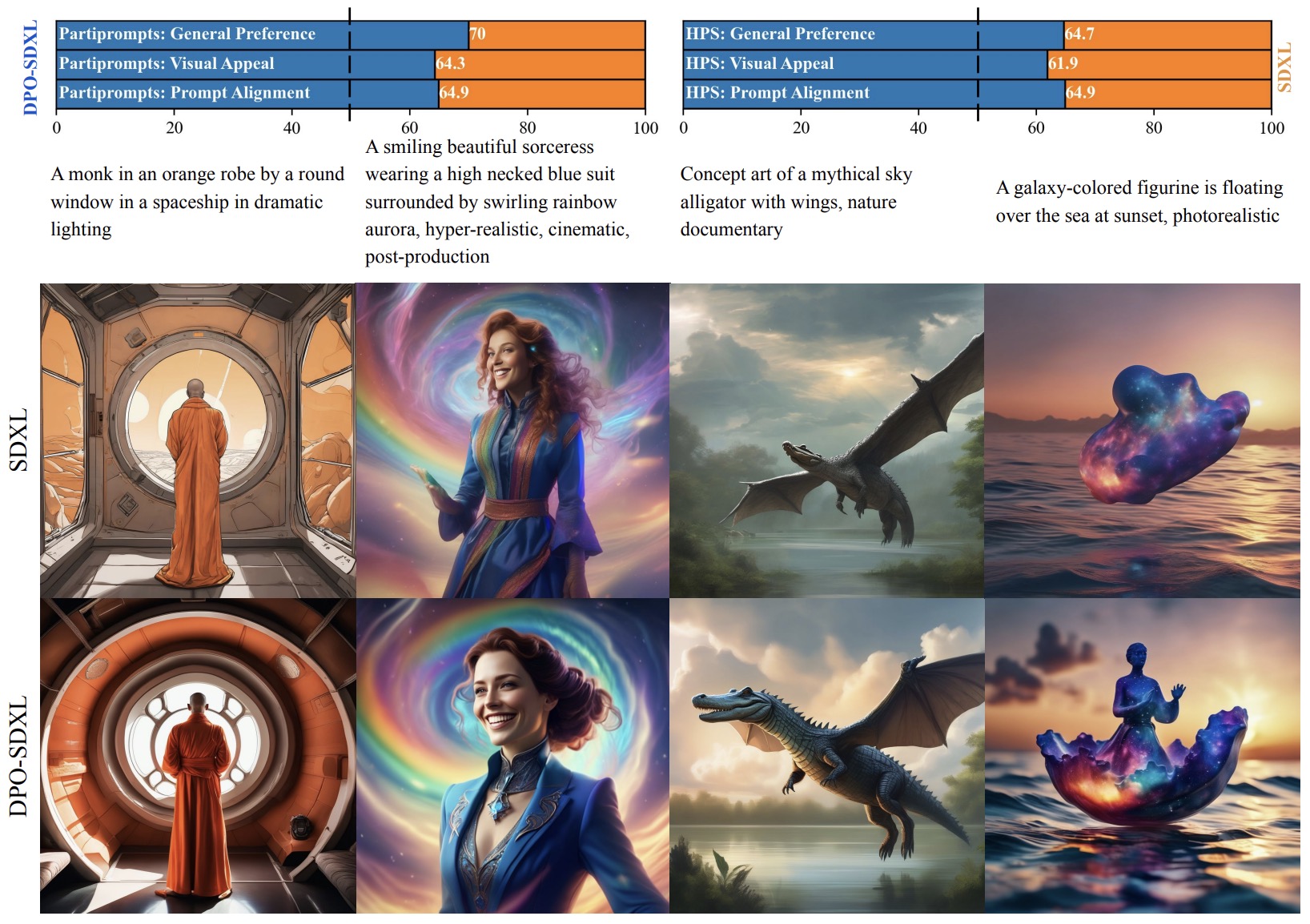
- Experiments demonstrate the effectiveness of Diffusion-DPO in various scenarios, including image-to-image editing and learning from AI feedback. The method significantly outperforms existing models in human evaluations for general preference, visual appeal, and prompt alignment.
- The paper’s findings indicate that Diffusion-DPO can effectively increase measured human appeal across an open vocabulary with stable training, without increased inference time, and improves generic text-image alignment.
- The authors note ethical considerations and risks associated with text-to-image generation, emphasizing the importance of diverse and representative sets of labelers and the potential biases inherent in the pre-trained models and labeling process.
- In summary, the paper presents a groundbreaking approach to align diffusion models with human preferences, demonstrating notable improvements in visual appeal and prompt alignment. It highlights the potential of direct preference optimization in the realm of text-to-image diffusion models and opens avenues for further research and application in this field.
Scalable Diffusion Models with Transformers
- This paper by Peebles and Xie from UC Berkeley and New York University introduces a new class of diffusion models that leverage the Transformer architecture for generating images. This innovative approach replaces the traditional convolutional U-Net backbone in latent diffusion models (LDMs) with a transformer operating on latent patches.
- Traditional diffusion models in image-level generative tasks predominantly use a convolutional U-Net architecture. However, the dominance of transformers in various domains like natural language processing and vision prompts this exploration of their use as a backbone for diffusion models.
- The paper proposes Diffusion Transformers (DiTs), which adhere closely to the standard Vision Transformer (ViT) model but with some vital tweaks. DiTs are designed to be faithful to standard transformer architecture, particularly the Vision Transformer (ViT) model, and are trained as latent diffusion models of images.
- Transformer Blocks and Design Space:
- DiTs process input tokens transformed from spatial representations of images (“patchify” process) through a sequence of transformer blocks.
- Four types of transformer blocks are explored: in-context conditioning, cross-attention block, adaptive layer norm (adaLN) block, and adaLN-Zero block. Each block processes additional conditional information like noise timesteps or class labels.
- The adaLN-Zero block, which initializes each DiT block as an identity function and modulates the activations immediately prior to any residual connections within the block, demonstrates the most efficient performance, achieving lower Frechet Inception Distance (FID) values than the other block types.
- The figure below from the paper shows the Diffusion Transformer (DiT) architecture. Left: We train conditional latent DiT models. The input latent is decomposed into patches and processed by several DiT blocks. Right: Details of our DiT blocks. We experiment with variants of standard transformer blocks that incorporate conditioning via adaptive layer norm, cross-attention and extra input tokens. Adaptive layer norm works best.
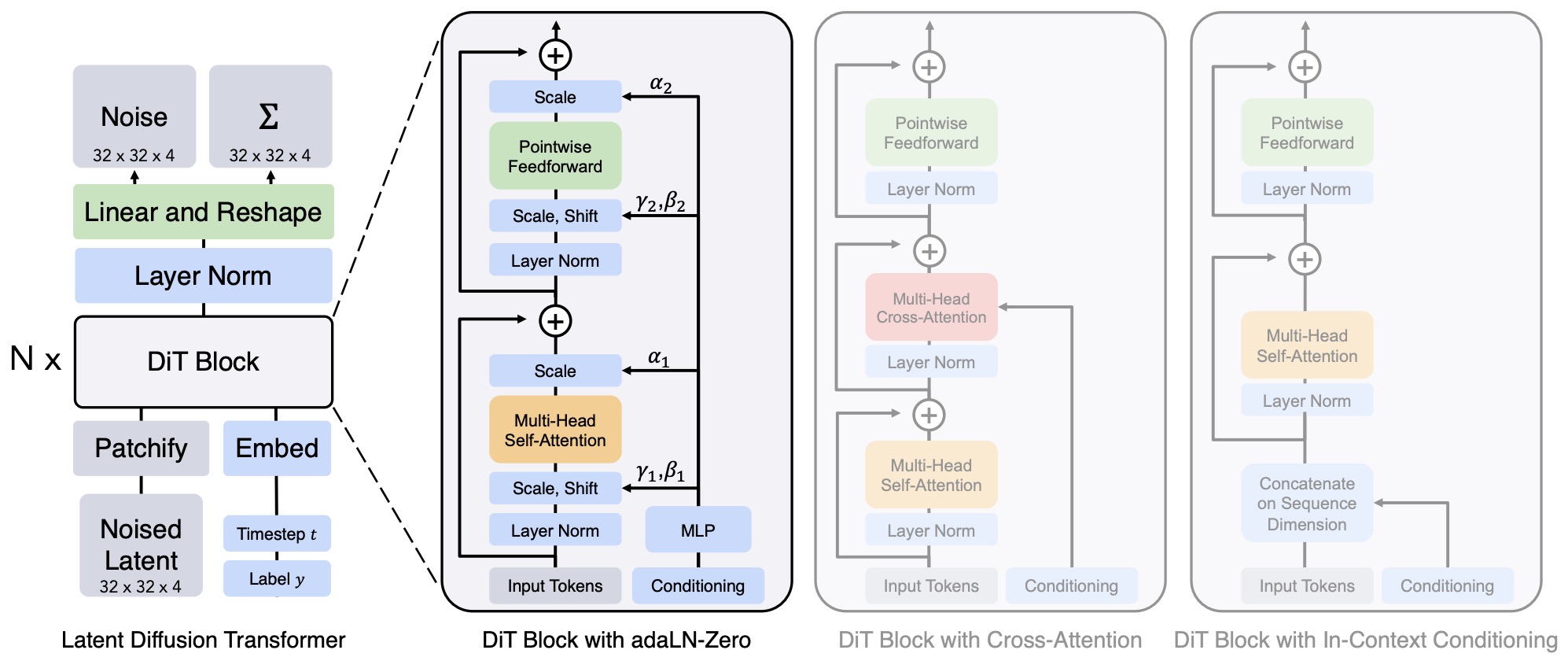
- Model Scaling and Performance:
- DiTs are scalable in terms of forward pass complexity, measured in GFLOPs. Different configurations (DiT-S, DiT-B, DiT-L, DiT-XL) cover a range of model sizes and computational complexities.
- Increasing model size and decreasing patch size significantly improves performance. FID scores improve as the transformer becomes deeper and wider, indicating that scaling model size (GFLOPs) is key to improved performance.
- The largest DiT-XL/2 models outperform all prior diffusion models, achieving a state-of-the-art FID of 2.27 on class-conditional ImageNet benchmarks at resolutions of 256 \(\times\) 256 and 512 \(\times\) 512.
- Implementation and Results: The models are trained using the AdamW optimizer. The DiT-XL/2 model, trained for 7 million steps, demonstrates high compute efficiency compared to both latent and pixel space U-Net models.
- Visual Quality: The paper highlights notable improvements in the visual quality of generated images with scaling in both model size and the number of tokens processed.
- Overall, the paper showcases the potential of transformer-based architectures in diffusion models, emphasizing scalability and compute efficiency, which contributes significantly to the field of generative models for images.
- Project page
DeepFloyd IF
- DeepFloyd, a part of Stability AI, has introduced DeepFloyd IF, a cutting-edge text-to-image cascaded pixel diffusion model known for its high photorealism and language understanding capabilities. This model is an open-source project and represents a significant advancement in text-to-image synthesis technology.
- DeepFloyd IF is built with multiple neural modules (independent neural networks that tackle specific tasks), joining forces within a single architecture to produce a synergistic effect.
- DeepFloyd IF generates high-resolution images in a cascading manner: the action kicks off with a base model that produces low-resolution samples, which are then boosted by a series of upscale models to create stunning high-resolution images, as shown in the figure (source) below.
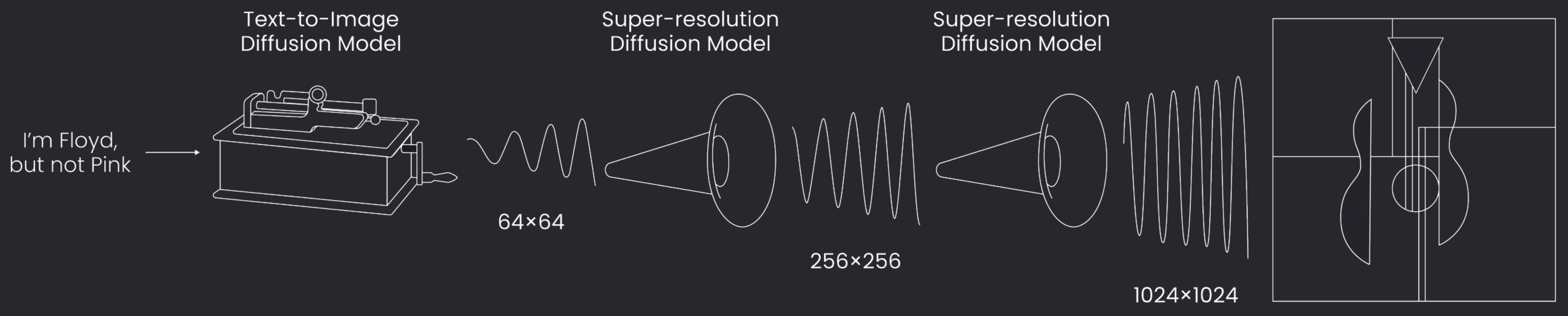
- DeepFloyd IF’s base and super-resolution models adopt diffusion models, making use of Markov chain steps to introduce random noise into the data, before reversing the process to generate new data samples from the noise.
- DeepFloyd IF operates within the pixel space, as opposed to latent diffusion (e.g. Stable Diffusion) that depends on latent image representations.
- The unique structure of DeepFloyd IF consists of a frozen text encoder and three cascaded pixel diffusion modules. The process begins with a base model generating a 64 \(\times\) 64 pixel image from a text prompt. This is followed by two super-resolution models, each escalating the resolution to 256 \(\times\) 256 pixels and then to 1024 \(\times\) 1024 pixels. All stages utilize a frozen text encoder based on the T5 transformer architecture, which extracts text embeddings. These embeddings are then input into a UNet architecture, which is enhanced with cross-attention and attention pooling features.
- The figure below from the paper shows the model architecture of DeepFloyd IF.
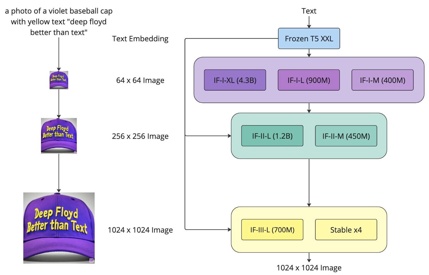
- The efficiency and effectiveness of DeepFloyd IF are evident in its performance, where it achieved a zero-shot FID score of 6.66 on the COCO dataset. This score is a testament to its state-of-the-art capabilities, outperforming other models in the domain. The success of DeepFloyd IF underscores the potential of larger UNet architectures in the initial stages of cascaded diffusion models and opens new avenues for future advancements in text-to-image synthesis.
- Code; Project page.
PIXART-\(\alpha\): Fast Training of Diffusion Transformer for Photorealistic Text-to-Image Synthesis
- The paper “PIXART-\(\alpha\): Fast Training of Diffusion Transformer for Photorealistic Text-to-Image Synthesis” by Chen et al. introduces PIXART-\(\alpha\), a transformer-based latent diffusion model for text-to-image (T2I) synthesis. This model competes with leading image generators such as SDXL, Imagen, and DALL-E 2 in quality, while significantly reducing training costs and CO2 emissions. Notably, it is also OPEN-RAIL licensed.
- Key Innovations:
- Efficient Architecture: PIXART-\(\alpha\) employs a Diffusion Transformer (DiT) with cross-attention modules, focusing on efficiency. This includes a streamlined class-condition branch and reparameterization for efficient training.
- Training Strategy Decomposition: The training is divided into three stages: learning pixel distributions, text-image alignment, and aesthetic enhancement.
- High-Informative Data: Utilizes an auto-labeling pipeline with LLaVA to create a dense, precise text-image dataset, improving the speed of text-image alignment learning.
- Technical Implementation:
- Text Encoding: Uses the T5-XXL model for advanced text encoding, enabling better handling of complex prompts.
- Pre-training and Stages: Incorporates pre-training on ImageNet, learning stages for pixel distribution, alignment, and aesthetics.
- Hardware Requirements: Initially requires 23GB GPU VRAM, but with diffusers, it can run under 7GB.
- The figure below from the paper shows the model architecture of PIXART-\(\alpha\). A cross-attention module is integrated into each block to inject textual conditions. To optimize efficiency, all blocks share the same adaLN-single parameters for time conditions.
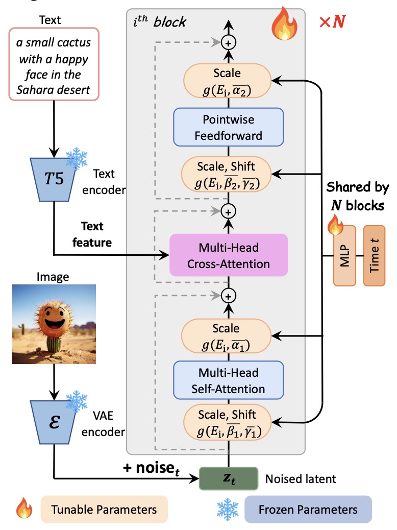
- Performance and Efficiency:
- Quality and Control: Delivers high-quality image synthesis with superior semantic control.
- Resource Efficiency: Achieves near state-of-the-art quality with only 2% of the training cost of other models, reducing CO2 emissions by 90%.
- Optimization Techniques: Implements shared normalization parameters (adaLN-single) and uses AdamW optimizer to enhance efficiency.
- Applications and Extensions: Showcases versatility through methods like DreamBooth and ControlNet, further expanding its practical applications.
- PIXART-\(\alpha\) represents a major advancement in T2I generation, offering a high-quality, efficient, and environmentally friendly solution. Its unique architecture and training strategy make it an innovative addition to the field of photorealistic T2I synthesis.
- Code; Hugging Face; Project page
RAPHAEL: Text-to-Image Generation via Large Mixture of Diffusion Paths
- This technical report by Xue et al. from the University of Hong Kong and SenseTime Research, the authors introduce RAPHAEL, a novel text-to-image diffusion model that generates highly artistic images closely aligned with textual prompts.
- RAPHAEL uniquely combines tens of mixture-of-experts (MoEs) layers, including space-MoE and time-MoE layers, allowing billions of diffusion paths. Each path intuitively functions as a “painter” for depicting specific textual concepts onto designated image regions at certain diffusion timesteps. This mechanism substantially enhances the precision in aligning text and image content.
- The authors report that RAPHAEL outperforms recent models like Stable Diffusion, ERNIE-ViLG 2.0, DeepFloyd, and DALL-E 2 in terms of image quality and aesthetic appeal. This is evidenced by superior performance in diverse styles (e.g., Japanese comics, realism, cyberpunk) and a state-of-the-art zero-shot FID score of 6.61 on the COCO dataset.
- An edge-supervised learning module is introduced to further refine image quality, focusing on maintaining intricate boundary details in various styles. RAPHAEL is implemented using a U-Net architecture with 16 transformer blocks, each containing a self-attention layer, a cross-attention layer, space-MoE, and time-MoE layers. The model, with three billion parameters, was trained on 1,000 A100 GPUs for two months.
- Framework of RAPHAEL. (a) Each block contains four primary components including a selfattention layer, a cross-attention layer, a space-MoE layer, and a time-MoE layer. The space-MoE is responsible for depicting different text concepts in specific image regions, while the time-MoE handles different diffusion timesteps. Each block uses edge-supervised cross-attention learning to further improve image quality. (b) shows details of space-MoE. For example, given a prompt “a furry bear under sky”, each text token and its corresponding image region (given by a binary mask) are directed through distinct space experts, i.e., each expert learns particular visual features at a region. By stacking several space-MoEs, we can easily learn to depict thousands of text concepts.
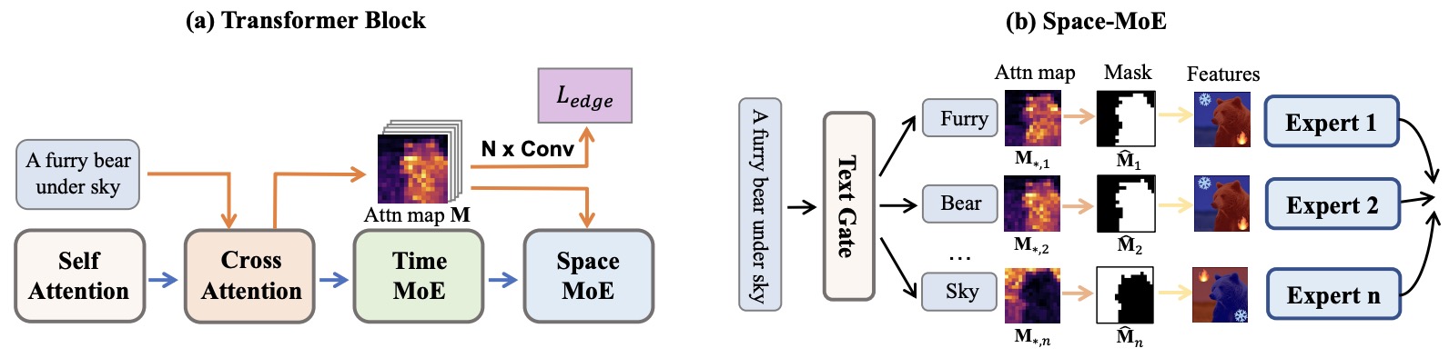
- The authors conducted extensive experiments, including a user study using the ViLG-300 benchmark, demonstrating RAPHAEL’s robustness and superiority in generating images that closely conform to the textual prompts. The study also showcases RAPHAEL’s flexibility in generating images of diverse styles and high resolutions up to 4096 \(\times\) 6144 when combined with a tailor-made SR-GAN model.
- RAPHAEL’s potential applications extend to various domains, with implications for both academic research and industry. The model’s limitations include the potential misuse for creating misleading or false information, a challenge common to powerful text-to-image generators.
- Project page
ERNIE-ViLG 2.0: Improving Text-to-Image Diffusion Model with Knowledge-Enhanced Mixture-of-Denoising-Experts
- This paper by Feng et al. from Baidu Inc. and Wuhan University of Science and Technology in CVPR 2023 focuses on enhancing text-to-image generation using diffusion models.
- They introduce ERNIE-ViLG 2.0, a large-scale Chinese text-to-image generation model, employing a diffusion-based approach with a 24B parameter scale. The model aims to significantly upgrade image quality and text relevancy.
- The model incorporates fine-grained textual and visual knowledge to improve semantic control and resolve object-attribute mismatching in image generation. This is achieved by using a text parser and an object detector to identify key elements in the text-image pair and aligning them in the learning process.
- Introduction of the Mixture-of-Denoising-Experts (MoDE) mechanism, which uses multiple specialized expert networks for different stages of the denoising process, allowing for more efficient handling of various denoising requirements at different steps.
- The figure below from the paper shows the architecture of ERNIE-ViLG 2.0, which incorporates fine-grained textual and visual knowledge of key elements in the scene and utilizes different denoising experts at different denoising stages.
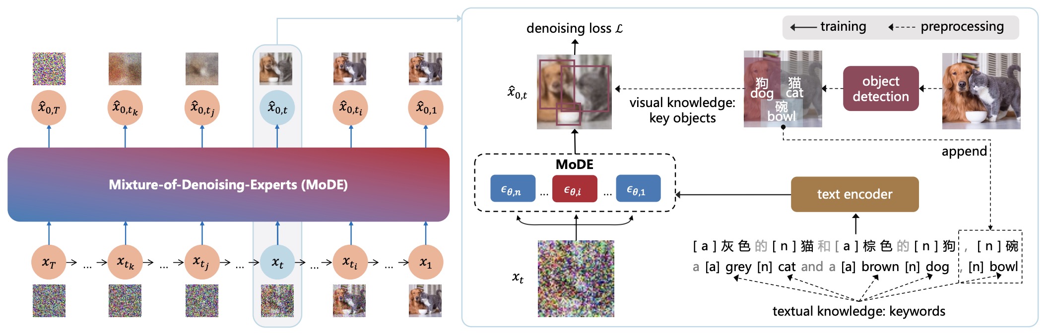
- ERNIE-ViLG 2.0 demonstrates state-of-the-art performance on MS-COCO with a zero-shot FID-30k score of 6.75. It also outperforms models like DALL-E 2 and Stable Diffusion in human evaluations using a bilingual prompt set, ViLG-300, for a fair comparison between English and Chinese text-to-image models.
- The model’s implementation involves a transformer-based text encoder with 1.3B parameters, 10 denoising U-Net experts with 2.2B parameters each, and training on 320 Tesla A100 GPUs for 18 days. The dataset comprises 170M image-text pairs, including English datasets translated into Chinese.
- Ablation studies and qualitative showcases confirm the effectiveness of the proposed knowledge enhancement strategies and the MoDE mechanism. The model shows improved handling of complex prompts, better sharpness, and texture in generated images.
- Future work includes enriching external image-text alignment knowledge and expanding the usage of multiple experts to advance generation capabilities. The paper also discusses potential risks and limitations related to data bias and model misuse in text-to-image generation.
- Project page
Imagen Video: High Definition Video Generation with Diffusion Models
- This paper by Ho et al. from Google Research, Brain Team, introduces Imagen Video, a text-conditional video generation system leveraging a cascade of video diffusion models. Imagen Video generates high-definition videos from text prompts using a base video generation model and a sequence of interleaved spatial and temporal super-resolution models.
- The core contributions and methodology of this work include the following technical details:
- Architecture and Components: Imagen Video utilizes a frozen T5 text encoder to process the text prompts, followed by a base video diffusion model and multiple spatial and temporal super-resolution (SSR and TSR) models. Specifically, the system comprises seven sub-models: one base video generation model, three SSR models, and three TSR models. This cascade structure allows the system to generate 1280x768 resolution videos at 24 frames per second, with a total of 128 frames (approximately 5.3 seconds).
- Diffusion Models: The diffusion models in Imagen Video are based on continuous-time formulations, with a forward process defined as a Gaussian process. The training objective is to denoise the latent variables through a noise-prediction loss. The v-parameterization is employed to predict noise, which ensures numerical stability and avoids color-shifting artifacts.
- Text Conditioning and Cascading: Text conditioning is achieved by injecting contextual embeddings from the T5-XXL text encoder into all models, ensuring alignment between the generated video and the text prompt. The cascading approach involves generating a low-resolution video first, which is then progressively enhanced through spatial and temporal super-resolution models. This method allows for high-resolution outputs without overly complex individual models.
- The following figure from the paper shows the cascaded sampling pipeline starting from a text prompt input to generating a 5.3-second, 1280 \(\times\) 768 video at 24fps. “SSR” and “TSR” denote spatial and temporal super-resolution respectively, and videos are labeled as frames \(\times\) width \(\times\) height. In practice, the text embeddings are injected into all models, not just the base model.
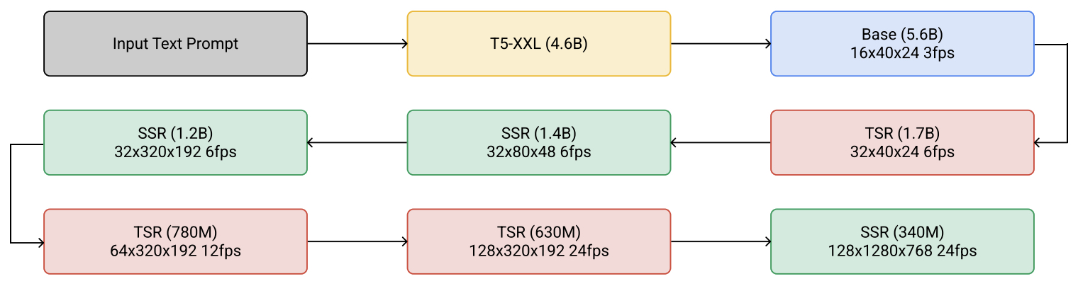
- Implementation Details:
- v-parameterization: Used for numerical stability and to avoid artifacts in high-resolution video generation.
- Conditioning Augmentation: Gaussian noise augmentation is applied to the conditioning inputs during training to reduce domain gaps and facilitate parallel training of different models in the cascade.
- Joint Training on Images and Videos: The models are trained on a mix of video-text pairs and image-text pairs, treating individual images as single-frame videos. This approach allows the model to leverage larger and more diverse image-text datasets.
- Classifier-Free Guidance: This method enhances sample fidelity and ensures that the generated video closely follows the text prompt by adjusting the denoising prediction.
- Progressive Distillation: This technique is used to speed up the sampling process. It involves distilling a trained DDIMs sampler into a model requiring fewer steps, thus significantly reducing computation time while maintaining sample quality.
- Experiments and Findings:
- The model shows high fidelity in video generation and can produce diverse content, including 3D object understanding and various artistic styles.
- Scaling the parameter count of the video U-Net leads to improved performance, indicating that video modeling benefits significantly from larger models.
- The v-parameterization outperforms ε-parameterization, especially at higher resolutions, due to faster convergence and reduced color inconsistencies.
- Distillation reduces sampling time by 18x, making the model more efficient without sacrificing perceptual quality.
- Conclusion: Imagen Video extends text-to-image diffusion techniques to video generation, achieving high-quality, temporally consistent videos. The integration of various advanced methodologies from image generation, such as v-parameterization, conditioning augmentation, and classifier-free guidance, demonstrates their effectiveness in the video domain. The work also highlights the potential for further improvements in video generation capabilities through continued research and development.
- Project page
Patch n’ Pack: NaViT, a Vision Transformer for any Aspect Ratio and Resolution
- This paper by Dehghani et al. from Google DeepMind introduces NaViT (Native Resolution ViT), a vision transformer designed to process images of arbitrary resolutions and aspect ratios without resizing them to a fixed resolution, which is common but suboptimal.
- NaViT leverages sequence packing during training, a technique inspired by natural language processing where multiple examples are packed into a single sequence, allowing efficient training on variable length inputs. This is termed Patch n’ Pack.
- Architectural Changes: NaViT builds on the Vision Transformer (ViT) but introduces masked self-attention and masked pooling to prevent different examples from attending to each other. It also uses factorized and fractional positional embeddings to handle arbitrary resolutions and aspect ratios. These embeddings are decomposed into separate embeddings for x and y coordinates and summed together, allowing for easy extrapolation to unseen resolutions.
- Training Enhancements: NaViT employs continuous token dropping, varying the token dropping rate per image, and resolution sampling, allowing mixed-resolution training by sampling from a distribution of image sizes while preserving aspect ratios. This enhances throughput and exposes the model to high-resolution images during training, yielding substantial performance improvements over equivalent ViTs.
- Efficiency: NaViT demonstrates significant computational efficiency, processing five times more images during training than ViT within the same compute budget. The O(n^2) cost of attention, a concern when packing multiple images into longer sequences, diminishes with model scale, making the attention cost a smaller proportion of the overall computation.
- The following figure from the paper shows an example packing enables variable resolution images with preserved aspect ratio, reducing training time, improving performance and increasing flexibility. We show here the aspects of the data preprocessing and modelling that need to be modified to support Patch n’ Pack. The position-wise operations in the network, such as MLPs, residual connections, and layer normalisations, do not need to be altered.
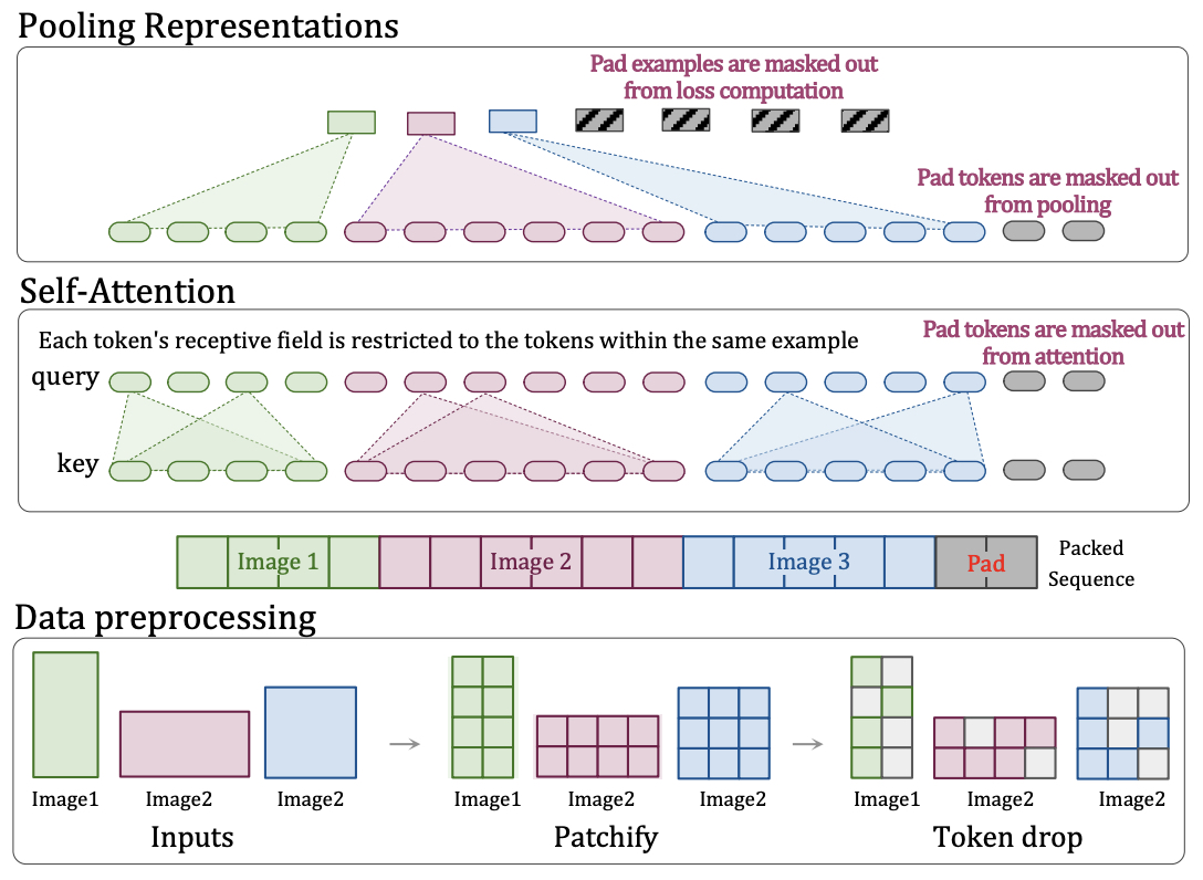
- Implementation: The authors implemented NaViT using a greedy packing approach to fix the final sequence lengths containing multiple examples. They addressed padding issues and example-level loss computation by modifying pooling heads to account for packing and using chunked contrastive loss to manage memory and time constraints.
- Performance: NaViT consistently outperforms ViT across various tasks, including image and video classification, object detection, and semantic segmentation. It shows improved results on robustness and fairness benchmarks, achieving better performance with lower computational costs and providing flexibility in handling different resolutions during inference.
- Evaluation: NaViT’s training and adaptation efficiency were evaluated through empirical studies on datasets like ImageNet, LVIS, WebLI, and ADE20k. The model demonstrated superior performance in terms of accuracy and computational efficiency, highlighting the benefits of preserving aspect ratios and using mixed-resolution training.
- NaViT represents a significant departure from the traditional convolutional neural network (CNN)-designed pipelines, offering a promising direction for Vision Transformers by enabling flexible and efficient processing of images at their native resolutions.
SDXL: Improving Latent Diffusion Models for High-Resolution Image Synthesis
- This paper by Podell et al. from Stability AI Applied Research details significant advancements in the field of text-to-image synthesis using latent diffusion models (LDMs).
- The paper introduces SDXL, a latent diffusion model that significantly improves upon previous versions of Stable Diffusion for text-to-image synthesis.
- SDXL incorporates a UNet architecture three times larger than its predecessors, primarily due to an increased number of attention blocks and a larger cross-attention context. This is achieved by using a second text encoder, significantly enhancing the model’s capabilities.
- Novel conditioning schemes are introduced, such as conditioning on original image resolution and cropping parameters. This conditioning is achieved through Fourier feature encoding and significantly improves the model’s performance and flexibility.
- SDXL is trained on multiple aspect ratios, a notable departure from standard square image outputs. This training approach allows the model to better handle images with varied aspect ratios, reflecting real-world data more accurately.
- An improved autoencoder is used, enhancing the fidelity of generated images, particularly in high-frequency details.
- The paper also discusses a refinement model used as a post-hoc image-to-image technique to further improve the visual quality of samples generated by SDXL. SDXL demonstrates superior performance compared to earlier versions of Stable Diffusion and rivals state-of-the-art black-box image generators. The model’s performance was validated through user studies and quantitative metrics.
- The figure below from the illustrates: (Left) Comparing user preferences between SDXL and Stable Diffusion 1.5 & 2.1. While SDXL already clearly outperforms Stable Diffusion 1.5 & 2.1, adding the additional refinement stage boosts performance. (Right) Visualization of the two-stage pipeline: They generate initial latents of size 128 \(\times\) 128 using SDXL. Afterwards, they utilize a specialized high-resolution refinement model and apply SDEdit on the latents generated in the first step, using the same prompt. SDXL and the refinement model use the same autoencoder.
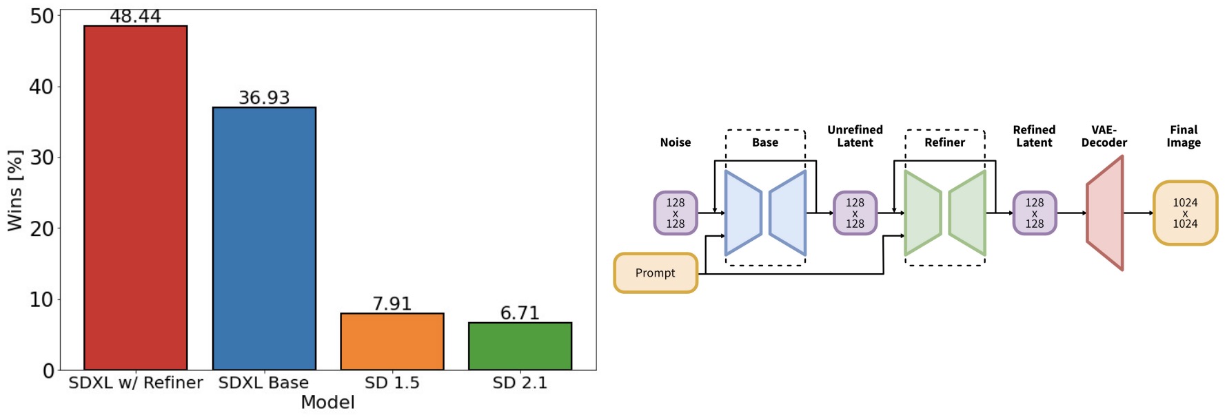
- The authors emphasize the open nature of SDXL, highlighting its potential to foster transparency in large model training and evaluation, which is crucial for responsible and ethical deployment of such technologies.
- The paper represents a significant step forward in generative modeling for high-resolution image synthesis, showcasing the potential of latent diffusion models in creating detailed and realistic images from textual descriptions.
Dreamix: Video Diffusion Models are General Video Editors
- Text-driven image and video diffusion models have recently achieved unprecedented generation realism. While diffusion models have been successfully applied for image editing, very few works have done so for video editing.
- This paper by Molad et al. from Google Research and The Hebrew University of Jerusalem presents the first diffusion-based method that is able to perform text-based motion and appearance editing of general videos. Our approach uses a video diffusion model to combine, at inference time, the low-resolution spatio-temporal information from the original video with new, high resolution information that it synthesized to align with the guiding text prompt.
- The following figure from the paper shows the video editing use-case with Dreamix: Frames from a video conditioned on the text prompt “A bear dancing and jumping to upbeat music, moving his whole body“. Dreamix transforms the eating monkey (top row) into a dancing bear, affecting appearance and motion (bottom row). It maintains fidelity to color, posture, object size and camera pose, resulting in a temporally consistent video.
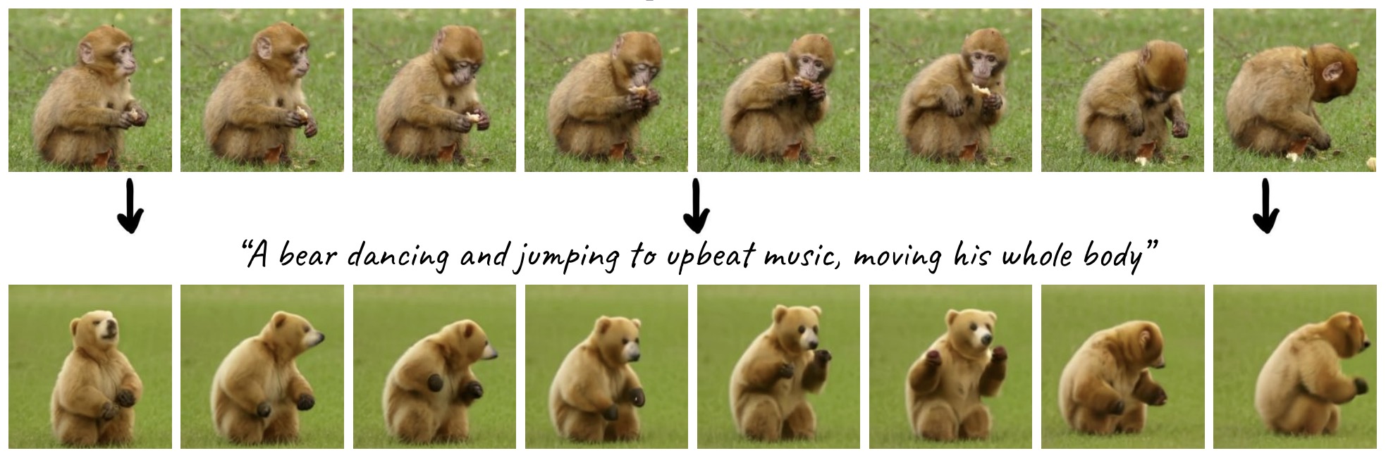
- As obtaining high-fidelity to the original video requires retaining some of its high-resolution information, we add a preliminary stage of finetuning the model on the original video, significantly boosting fidelity.
- They propose to improve motion editability by a new, mixed objective that jointly finetunes with full temporal attention and with temporal attention masking.
- They further introduce a new framework for image animation. They first transform the image into a coarse video by simple image processing operations such as replication and perspective geometric projections, and then use their general video editor to animate it.
- As a further application, Dreamix can be used for subject-driven video generation. Extensive qualitative and numerical experiments showcase the remarkable editing ability of Dreamix and establish its superior performance compared to baseline methods.
- The following figure from the paper illustrates the process of inference. Dreamix supports multiple applications by application dependent pre-processing (left), converting the input content into a uniform video format. For image-to-video, the input image is duplicated and transformed using perspective transformations, synthesizing a coarse video with some camera motion. For subject-driven video generation, the input is omitted - finetuning alone takes care of the fidelity. This coarse video is then edited using their general “Dreamix Video Editor“ (right): we first corrupt the video by downsampling followed by adding noise. We then apply the finetuned text-guided VDM, which upscales the video to the final spatio-temporal resolution.
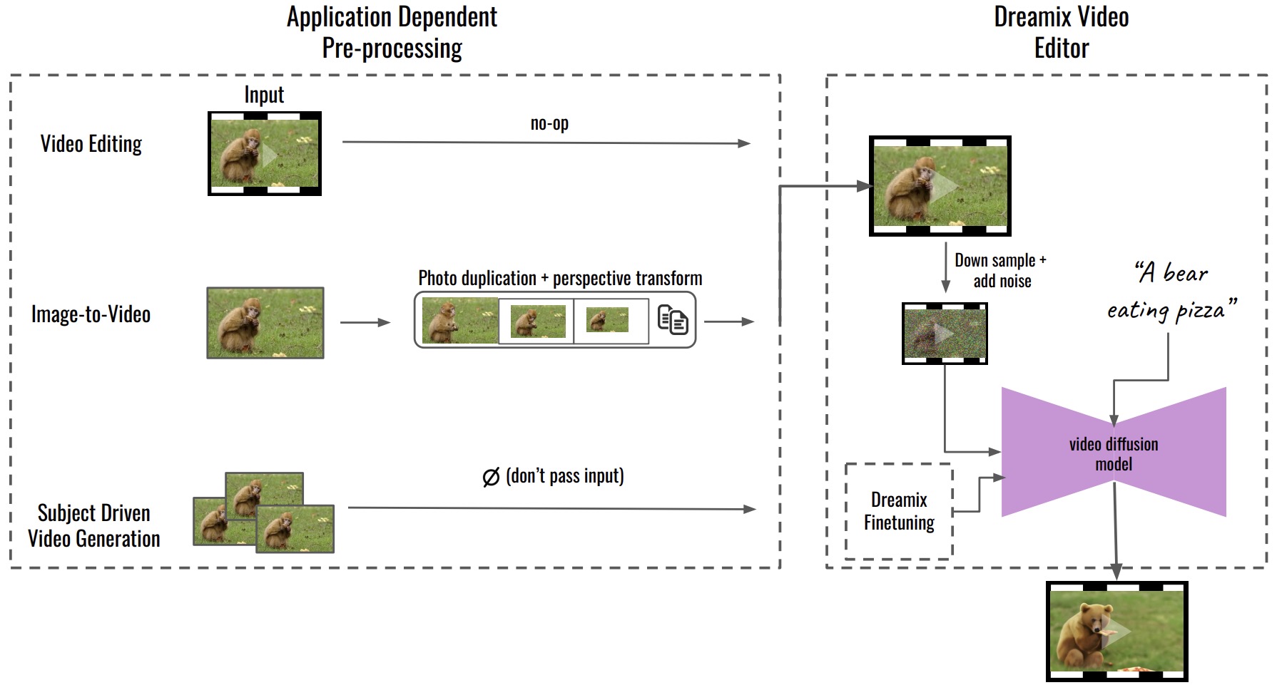
Stable Video Diffusion: Scaling Latent Video Diffusion Models to Large Datasets
- This paper by Blattmann et al. from Stability AI introduces Stable Video Diffusion (SVD), a latent video diffusion model designed for high-resolution text-to-video and image-to-video generation. They address the challenge of lacking a unified strategy for curating video data and propose a methodical curation process for training successful video LDMs, which includes three stages:
- Stage I: Text-to-image (or simply, image pretraining), i.e., a 2D text-to-image diffusion model.
- Stage II: video pretraining, which trains on large amounts of videos.
- Stage III: video finetuning, which refines the model on a small subset of high-quality videos at higher resolution.
- In the initial stage, leveraging insights from large-scale image model training, the authors curated an extensive pretraining dataset named LVD, consisting of approximately 580 million annotated video clip pairs. This dataset underwent rigorous processing, including cut detection and annotation using several methods such as image captioning and optical flow analysis, to filter out low-quality content. Specifically, to avoid the samples in the dataset that can be expected to degrade the performance of the final video model, such as clips with less motion, excessive text presence, or generally low aesthetic value, they therefore additionally annotate the dataset with dense optical flow calculated at 2 FPS, with which static scenes are filtered out by removing any videos whose average optical flow magnitude is below a certain threshold.
- The following figure from the paper shows that the initial dataset contains many static scenes and cuts which hurts training of generative video models. Left: Average number of clips per video before and after our processing, revealing that our pipeline detects lots of additional cuts. Right: The distribution of average optical flow score for one of these subsets before processing, which contains many static clips.
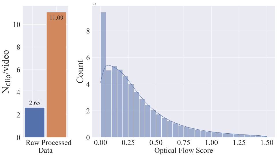
- The paper outlines the importance of each training stage and demonstrates that systematic data curation significantly boosts model performance. Notably, they emphasize the necessity of pretraining on a well-curated dataset for generating high-quality videos, showing that models pretrained in this manner outperform others when finetuned on smaller, high-quality datasets.
- Leveraging the curated dataset, the authors trained a base model that provides a comprehensive motion representation. This base model was further finetuned for several applications, including text-to-video and image-to-video generation, demonstrating state-of-the-art performance. The model also supports controlled camera motion through LoRA modules and has been shown to serve as a robust multi-view 3D prior, capable of generating multiple consistent views of an object in a feedforward manner.
- The SVD model stands out for its ability to efficiently generate high-fidelity videos from both text and images, offering a substantial advancement over existing methods in terms of visual quality and consistency. The authors released the code and model weights, contributing a valuable resource to the research community for further exploration and development in video generation technology.
- Blog; Code; Hugging Face
Fine-tuning Diffusion Models
- Per Using LoRA for Efficient Stable Diffusion Fine-Tuning, Low-Rank Adaptation (LoRA) can be used for efficient fine-tuning of large language models, originally introduced by Microsoft researchers.
- LoRA involves freezing pre-trained model weights and adding trainable layers to reduce the number of parameters and GPU memory requirements. It has been applied to Stable Diffusion fine-tuning, particularly in cross-attention layers.
- The technique enables quicker and less computationally intensive training, resulting in much smaller trained weights. The article also covers the use of LoRA in diffusers for Dreambooth and full fine-tuning methods, highlighting the reduced training time and lower computational requirements.
- Additionally, it introduces methods like Textual Inversion and Pivotal Tuning, which are complementary to LoRA. The page includes code snippets for using LoRA in Stable Diffusion fine-tuning and Dreambooth training.
Diffusion Model Alignment
Diffusion Model Alignment Using Direct Preference Optimization
- This paper by Wallace et al. from Salesforce AI and Stanford University proposes a novel method for aligning diffusion models to human preferences.
- The paper introduces Diffusion-DPO, a method adapted from DPO, for aligning text-to-image diffusion models with human preferences. This approach is a significant shift from typical language model training, emphasizing direct optimization on human comparison data.
- Unlike typical methods that fine-tune pre-trained models using curated images and captions, Diffusion-DPO directly optimizes a policy that best satisfies human preferences under a classification objective. It re-formulates DPO to account for a diffusion model notion of likelihood using the evidence lower bound, deriving a differentiable objective.
- The authors utilized the Pick-a-Pic dataset, comprising 851K crowdsourced pairwise preferences, to fine-tune the base model of the Stable Diffusion XL (SDXL)-1.0 model with Diffusion-DPO. The fine-tuned model showed significant improvements over both the base SDXL-1.0 and its larger variant in terms of visual appeal and prompt alignment, as evaluated by human preferences.
- The paper also explores a variant of the method that uses AI feedback, showing comparable performance to training on human preferences. This opens up possibilities for scaling diffusion model alignment methods.
- The figure below from paper illustrates: (Top) DPO-SDXL significantly outperforms SDXL in human evaluation. (L) PartiPrompts and (R) HPSv2 benchmark results across three evaluation questions, majority vote of 5 labelers. (Bottom) Qualitative comparisons between SDXL and DPO-SDXL. DPOSDXL demonstrates superior prompt following and realism. DPO-SDXL outputs are better aligned with human aesthetic preferences, favoring high contrast, vivid colors, fine detail, and focused composition. They also capture fine-grained textual details more faithfully.
- Experiments demonstrate the effectiveness of Diffusion-DPO in various scenarios, including image-to-image editing and learning from AI feedback. The method significantly outperforms existing models in human evaluations for general preference, visual appeal, and prompt alignment.
- The paper’s findings indicate that Diffusion-DPO can effectively increase measured human appeal across an open vocabulary with stable training, without increased inference time, and improves generic text-image alignment.
- The authors note ethical considerations and risks associated with text-to-image generation, emphasizing the importance of diverse and representative sets of labelers and the potential biases inherent in the pre-trained models and labeling process.
- In summary, the paper presents a groundbreaking approach to align diffusion models with human preferences, demonstrating notable improvements in visual appeal and prompt alignment. It highlights the potential of direct preference optimization in the realm of text-to-image diffusion models and opens avenues for further research and application in this field.
Further Reading
The Illustrated Stable Diffusion
- Jay Alammar’s (of The Illustrated Transformer fame) article explaining Stable Diffusion.
Understanding Diffusion Models: A Unified Perspective
- This tutorial paper by Calvin Luo from Google Brain goes from the basics of ELBO, VAE, and hierarchical VAE to diffusion models.
The Annotated Diffusion Model
- This blog post by HugginFace takes a deeper look into Denoising Diffusion Probabilistic Models (also known as DDPMs, diffusion models, score-based generative models or simply autoencoders) as researchers have been able to achieve remarkable results with them for generative models. It goes over the original DDPM paper (Ho et al., 2020), implementing it step-by-step in PyTorch, based on Phil Wang’s implementation - which itself is based on the original TensorFlow implementation.
Lilian Weng: What are Diffusion Models?
- This tutorial paper by Lilian Weng from OpenAI covers the math behind diffusion models in detail.
Stable Diffusion - What, Why, How?
- This YouTube video by Edan Meyer explains how Stable Diffusion works at a high level, briefly talks about how it is different from other Diffusion-based models, compares it to DALL-E 2, and digs into the code.
How does Stable Diffusion work? – Latent Diffusion Models Explained
- This YouTube video by Letitia covers diffusion models, injecting text to generate images (conditional generation), and stable diffusion as a latent diffusion model.
Diffusion Explainer
-
Diffusion Explainer, an interactive web application, is designed to visually demonstrate the process of transforming a text prompt into high-resolution images within seconds.
- The app offers the following features for exploration:
- Text representation generation: Observe how your text prompt is tokenized and converted into numerical vectors, which guide the creation of images.
- Image representation refinement: Witness the transformation of random noise into a coherent image through successive steps.
- Image upscaling: Discover how the final image representation is enhanced into high-resolution output based on your input.
- With its interactive controls, you can modify prompts, adjust seeds, and tweak guidance scales, allowing you to see how each factor influences the final image. This tool is ideal for those seeking a deeper understanding of diffusion models and text-to-image generation technologies.

Jupyter notebook on the theoretical and implementation aspects of Score-based Generative Models (SGMs)
- Great technical explanation and implementation (along with a JAX implementation) of score-based generative models (SGMs), also called diffusion models.
References
- Diffusion models Vs GANs: Which one to choose for Image Synthesis
- Diffusion models
- Introduction to Diffusion Models for Machine Learning
- What are Diffusion Models?
- Denoising Diffusion Probabilistic Models by Ho et. al
- Lil’Log: Diffusion Models
- Assembly AI: Diffusion Models for Machine Learning Introduction
- Google ML Crashcourse on GANs
- Wikipedia: Markov Chain
- AI Summer: Latent Variable Models
- Diffusion Models Beat GANs on Image Synthesis
- Jay Alammar’s Stable Diffusion Twitter thread
- Hugging Face Stable Diffusion
- Towards Data Science: DALL-E 2 Explained
- Hugging Face’s Training with Diffusers notebook
- Hugging Face Diffusers Intro notebook
Citation
If you found our work useful, please cite it as:
@article{Chadha2020DistilledDiffusionModels,
  title   = {Diffusion Models},
  author  = {Chadha, Aman and Jain, Vinija},
  journal = {Distilled AI},
  year    = {2020},
  note    = {\url{https://aman.ai}}
}