Models • Diffusion Models
- Background
- Overview
- Introduction
- Advantages
- Definitions
- 🧨 Diffusion models: A Deep Dive
- Training
- Model Choices
- Network Architecture
- Final Objective
- Diffusion Model Theory Summary
- Diffusion models in PyTorch 👩🏽💻
- HuggingFace Diffusers
- Implementations
- Gallery
- Final Words
- References
- Further Reading
- Citation
Background
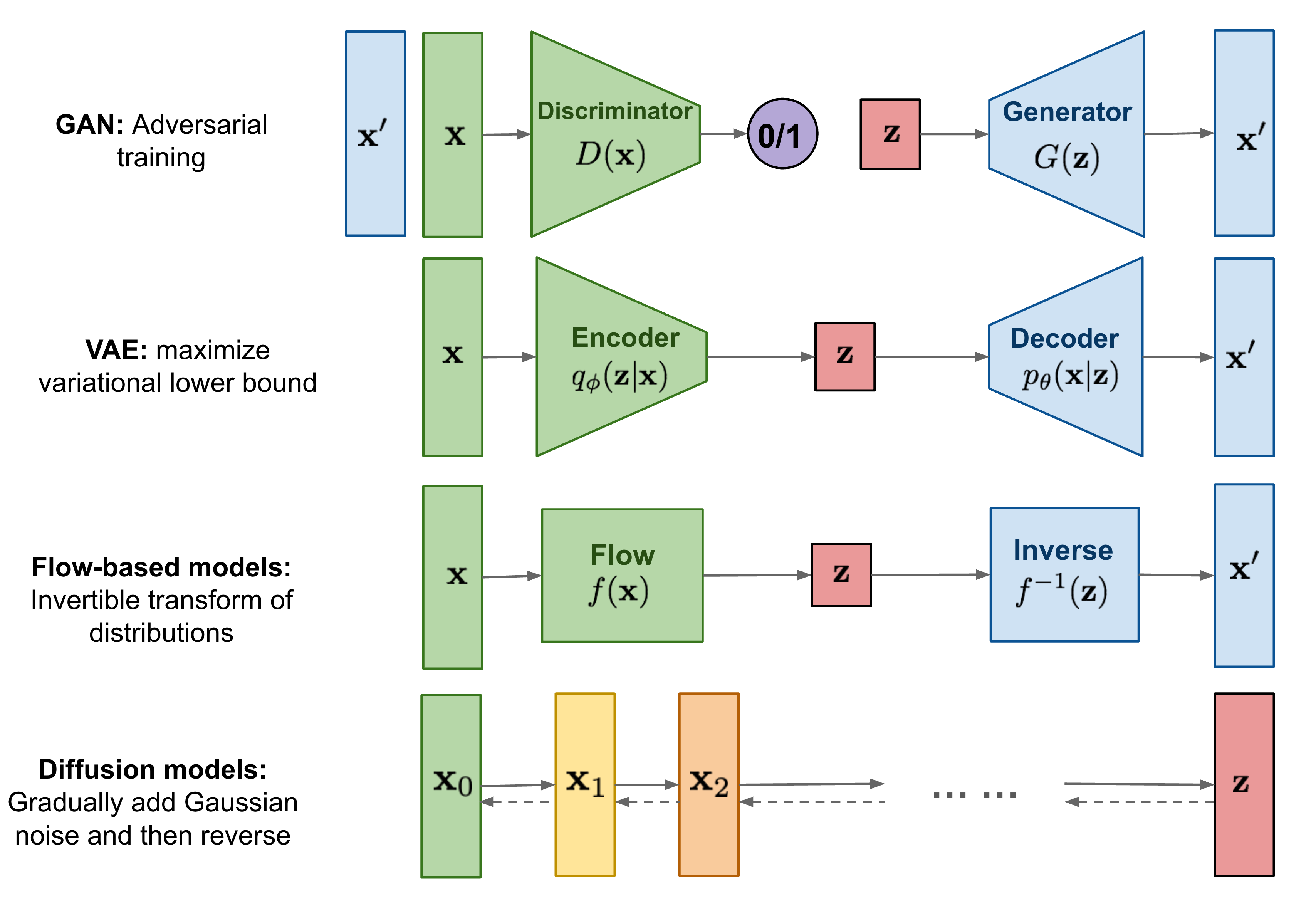
- There are three common types of generative models, GAN, VAE, and Flow-based models. They have shown great success in generating high-quality samples, but each has some limitations of its own. GAN models are known for potentially unstable training and less diversity in generation due to their adversarial training nature. VAE relies on a surrogate loss. Flow models have to use specialized architectures to construct reversible transform.
- Diffusion models are inspired by non-equilibrium thermodynamics. They define a Markov chain of diffusion steps to slowly add random noise to data and then learn to reverse the diffusion process to construct desired data samples from the noise. Unlike VAE or flow models, diffusion models are learned with a fixed procedure and the latent variable has high dimensionality (same as the original data).
- The following diagram from Lilian Weng’s blog provides an overview of the different types of generative models:
Overview
- The meteoric rise of diffusion models is one of the biggest developments in Machine Learning in the past several years.
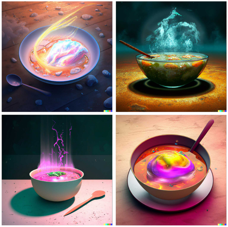
- Diffusion models are generative models which have been gaining significant popularity in the past several years, and for good reason. A handful of seminal papers released in the 2020s alone have shown the world what Diffusion models are capable of, such as beating GANs on image synthesis. Most recently, Diffusion models were used in DALL-E 2, OpenAI’s image generation model (image below generated using DALL-E 2).
- Given the recent wave of success by Diffusion models, many Machine Learning practitioners are surely interested in their inner workings.
- In this article, we will examine the theoretical foundations for Diffusion models, and then demonstrate how to generate images with a diffusion model in PyTorch. Let’s dive in!
Introduction
- Diffusion probabilistic models (also simply called diffusion models) are generative models, meaning that they are used to generate data similar to the data on which they are trained. As the name suggests, generative models are used to generate new data, for e.g., they can generate new photos of animals that look like real animals whereas discriminative models could tell apart a cat from a dog.
- “They are a class of latent variable models trained variational inference. What this means in practice is that we train a deep neural network to denoise images blurred with some sort of noise function.” Source
- Diffusion models are essentially deep neural networks that are trained to denoise images that have been blurred intentionally and thus, as a result, have better understanding of the image.

- Fundamentally, diffusion models work by destroying training data through the successive addition of Gaussian noise, and then learning to recover the data by reversing this noising process. In other words, diffusion models are parameterized Markov chains models trained to gradually denoise data. After training, we can use the diffusion model to generate data by simply passing randomly sampled noise through the learned denoising process. In other words, diffusion models undergo the process of transforming a random collection of numbers (the “latents tensor”) into a processed collection of numbers containing the right image information.
- Diffusion Models also go by Diffusion Probabilistic Models, score-based generative models or in some contexts, have been compared to denoising autoencoders owing to similarity in behavior.
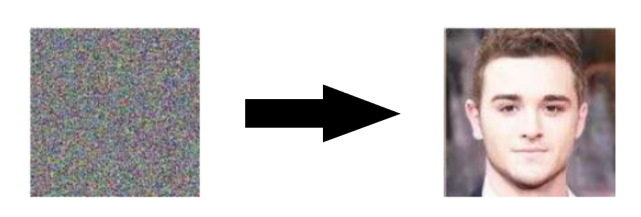
- The following diagram shows that diffusion models can be used to generate images from noise (figure modified from source):
- More specifically, a diffusion model is a latent variable model which maps to the latent space using a fixed Markov chain. This chain gradually adds noise to the data in order to obtain the approximate posterior \(q\left(\mathbf{x} 1: T \mid \mathbf{x}_{0}\right)\), where \(\mathbf{x} 1, \ldots, \mathbf{x} T\) are the latent variables with the same dimensionality as \(\mathbf{x}_{0}\). In the figure below, we see such a Markov chain manifested for image data.
- The following diagram (figure modified from source):

- Ultimately, the image is asymptotically transformed to pure Gaussian noise. The goal of training a diffusion model is to learn the reverse process - i.e. training \(p_{\theta}\left(x_{t-1} \mid x_{t}\right)\). By traversing backwards along this chain, we can generate new data, as shown below (figure modified from source).

- Under-the-hood, diffusion Models define a Markov chain of diffusion steps that add random noise to the data and then learn to reverse the diffusion process in order to create the desired data output from the noise. This can be seen in the image below:
- Recall that a Markov chain is a stochastic model that describes a sequence of possible events where the probability of each event only depends on the state of the previous event. Markov chains are used to calculate the probability of an event occurring by considering it as a state transitioning to another state or a state transitioning to the same state as before. The defining characteristic of a Markov chain is that no matter how the process arrived at its present state, the possible future states are fixed.
- Key takeaway
- In a nutshell, diffusion models are constructed by first describing a procedure for gradually turning data into noise, and then training a neural network that learns to invert this procedure step-by-step. Each of these steps consists of taking a noisy input and making it slightly less noisy, by filling in some of the information obscured by the noise. If you start from pure noise and do this enough times, it turns out you can generate data this way! (source)
Advantages
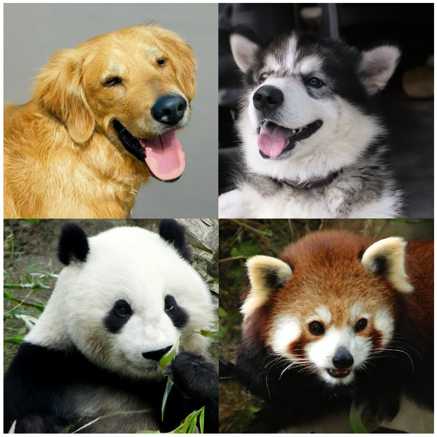
- Diffusion probabilistic models are latent variable models capable to synthesize high quality images. As mentioned above, research into diffusion models has exploded in recent years. Inspired by non-equilibrium thermodynamics, diffusion models currently produce State-of-the-Art image quality, examples of which can be seen below (figure adapted from source):
- Beyond cutting-edge image quality, diffusion models come with a host of other benefits, including not requiring adversarial training. The difficulties of adversarial training are well-documented; and, in cases where non-adversarial alternatives exist with comparable performance and training efficiency, it is usually best to utilize them. On the topic of training efficiency, diffusion models also have the added benefits of scalability and parallelizability.
- While diffusion models almost seem to be producing results out of thin air, there are a lot of careful and interesting mathematical choices and details that provide the foundation for these results, and best practices are still evolving in the literature. Let’s take a look at the mathematical theory underpinning diffusion models in more detail now.
- Their performance is, allegedly, superior to recent state-of-the-art generative models like Generative Adversarial Networks (GANs) and Variational Autoencoders (VAEs) in most cases.
Definitions
Diffusion Models
- Diffusion models are neural models that model \(p_{\theta}\left(\mathbf{x}_{t-1} \mid \mathbf{x}_{t}\right)\) and are trained end-to-end to denoise a noisy input to a continuous output such as an image/audio (similar to how GANs generate continuous outputs). Examples: UNet, Conditioned UNet, 3D UNet, Transformer UNet.
- The following figure from the DDPM paper shows the process of a diffusion model:

Schedulers
- Algorithm class for both inference and training. The class provides functionality to compute previous image according to alpha, beta schedule as well as predict noise for training. Examples: DDPM, DDIM, PNDM, DEIS.
- The figure below from the DDPM paper shows the sampling and training algorithms:

Sampling and training algorithms
- Diffusion Pipeline: End-to-end pipeline that includes multiple diffusion models, possible text encoders, super-resolution model (for high-res image generation, in case of Imagen), etc.
- Examples: GLIDE, Latent-Diffusion, Imagen, DALL-E 2.
- The figure below from the Imagen paper shows the overall flow of the model.

🧨 Diffusion models: A Deep Dive
🖼 General overview
- Diffusion Models are a latent variable model that maps the latent space using the Markov chain. They essentially are made up of neural networks that learn to gradually de-noise data.
- Note: Latent variable models aim to model the probability distribution with latent variables. Latent variables are a transformation of the data points into a continuous lower-dimensional space. (source)
- Additionally, the latent space is simply a representation of compressed data in which similar data points are closer together in space.
- Latent space is useful for learning data features and for finding simpler representations of data for analysis.
- Diffusion models consist of two processes: a predefined forward diffusion and a learned reverse de-noising diffusion process.
- In the image below, we can see the Markov chain working towards image generation. It represents the first process of forward diffusion.
- The forward diffusion process \(q\) of our choosing, gradually adds Gaussian noise to an image, until you end up with pure noise.

- Next, the image is asymptotically transformed to just Gaussian noise. The goal of training a diffusion model is to learn the reverse process.
- The second process below is the learned reverse de-noising diffusion process \(p_\theta\). Here, a neural network is trained to gradually de-noise an image starting from pure noise, until you end up with an actual image.
- Thus, we traverse backwards along this chain to generate the new data as seen below:

- Both the forward and reverse process (both indexed with \(t\)) continue for a duration of finite time steps \(T\) (the DDPM authors use \(T\) =1000).
- You will start off with \(t = 0\) where you will sample a real image \(x_0\) from your data distribution.
- A quick example is say you have an image of a cat from ImageNet dataset.
- You will then continue with the forward process and sample some noise from a Gaussian distribution at each time step \(t\).
- This will be added to the image of the previous time step.
- Given a sufficiently large \(T\) and a continuous process of adding noise at each time step, you will end up with \(t = T\).
-
This is also called an isotropic Gaussian distribution.
- Below is the high-level overview of how everything runs under the hood:
- we take a random sample \(x_0\) from the real unknown and complex data distribution \(q(x_0)\)
- we sample a noise level \(t\) uniformly between \(1\) and \(T\) (i.e., a random time step)
- we sample some noise from a Gaussian distribution and corrupt the input by this noise at level \(t\) (using the nice property defined above)
- the neural network is trained to predict this noise based on the corrupted image \(x_t\) (i.e. noise applied on \(x_0\) based on known schedule \(\beta_t\)) In reality, all of this is done on batches of data, as one uses stochastic gradient descent to optimize neural networks.
🧮 The Under-the-hood Math
-
As mentioned above, a diffusion model consists of a forward process (or diffusion process), in which a datum (generally an image) is progressively noised, and a reverse process (or reverse diffusion process), in which noise is transformed back into a sample from the target distribution.
-
The sampling chain transitions in the forward process can be set to conditional Gaussians when the noise level is sufficiently low. Combining this fact with the Markov assumption leads to a simple parameterization of the forward process:
\[q\left(\mathbf{x}_{1: T} \mid \mathbf{x}_{0}\right):=\prod_{t=1}^{T} q\left(\mathbf{x}_{t} \mid \mathbf{x}_{t-1}\right):=\prod_{t=1}^{T} \mathcal{N}\left(\mathbf{x}_{t} ; \sqrt{1-\beta_{t}} \mathbf{x}_{t-1}, \beta_{t} \mathbf{I}\right)\]- where \(\beta_1, \ldots, \beta_T\) is a variance schedule (either learned or fixed) which, if well-behaved, ensures that \(x_T\) is nearly an isotropic Gaussian for sufficiently large \(T\).
-
Given the Markov assumption, the joint distribution of the latent variables is the product of the Gaussian conditional chain transitions (figure modified from source).

-
As mentioned previously, the “magic” of diffusion models comes in the reverse process. During training, the model learns to reverse this diffusion process in order to generate new data. Starting with the pure Gaussian noise \(p(\mathbf{x} T):=\mathcal{N}\left(\mathbf{x}_{T}, \mathbf{0}, \mathbf{I}\right)\), the model learns the joint distribution \(p \theta(\mathbf{x} 0: T)\) as,
\[p_{\theta}\left(\mathbf{x}_{0: T}\right):=p\left(\mathbf{x}_{T}\right) \prod_{t=1}^{T} p_{\theta}\left(\mathbf{x}_{t-1} \mid \mathbf{x}_{t}\right):=p\left(\mathbf{x}_{T}\right) \prod_{t=1}^{T} \mathcal{N}\left(\mathbf{x}_{t-1} ; \boldsymbol{\mu}_{\theta}\left(\mathbf{x}_{t}, t\right), \boldsymbol{\Sigma}_{\theta}\left(\mathbf{x}_{t}, t\right)\right)\]- where the time-dependent parameters of the Gaussian transitions are learned. Note in particular that the Markov formulation asserts that a given reverse diffusion transition distribution depends only on the previous timestep (or following timestep, depending on how you look at it):

Training
- A diffusion model is trained by finding the reverse Markov transitions that maximize the likelihood of the training data. In practice, training equivalently consists of minimizing the variational upper bound on the negative log likelihood.
-
Notation Detail: Note that \(L_{v l b}\) is technically an upper bound (the negative of the ELBO) which we are trying to minimize, but we refer to it as \(L_{v l b}\) for consistency with the literature.
-
We seek to rewrite the \(L_{v l b}\) in terms of Kullback-Leibler (KL) Divergences. The KL Divergence is an asymmetric statistical distance measure of how much one probability distribution \(P\) differs from a reference distribution \(Q\). We are interested in formulating \(L_{v l b}\) in terms of \(KL\) divergences because the transition distributions in our Markov chain are Gaussians, and the KL divergence between Gaussians has a closed form.
Recap: KL Divergence
-
The mathematical form of the \(\mathrm{KL}\) divergence for continuous distributions is,
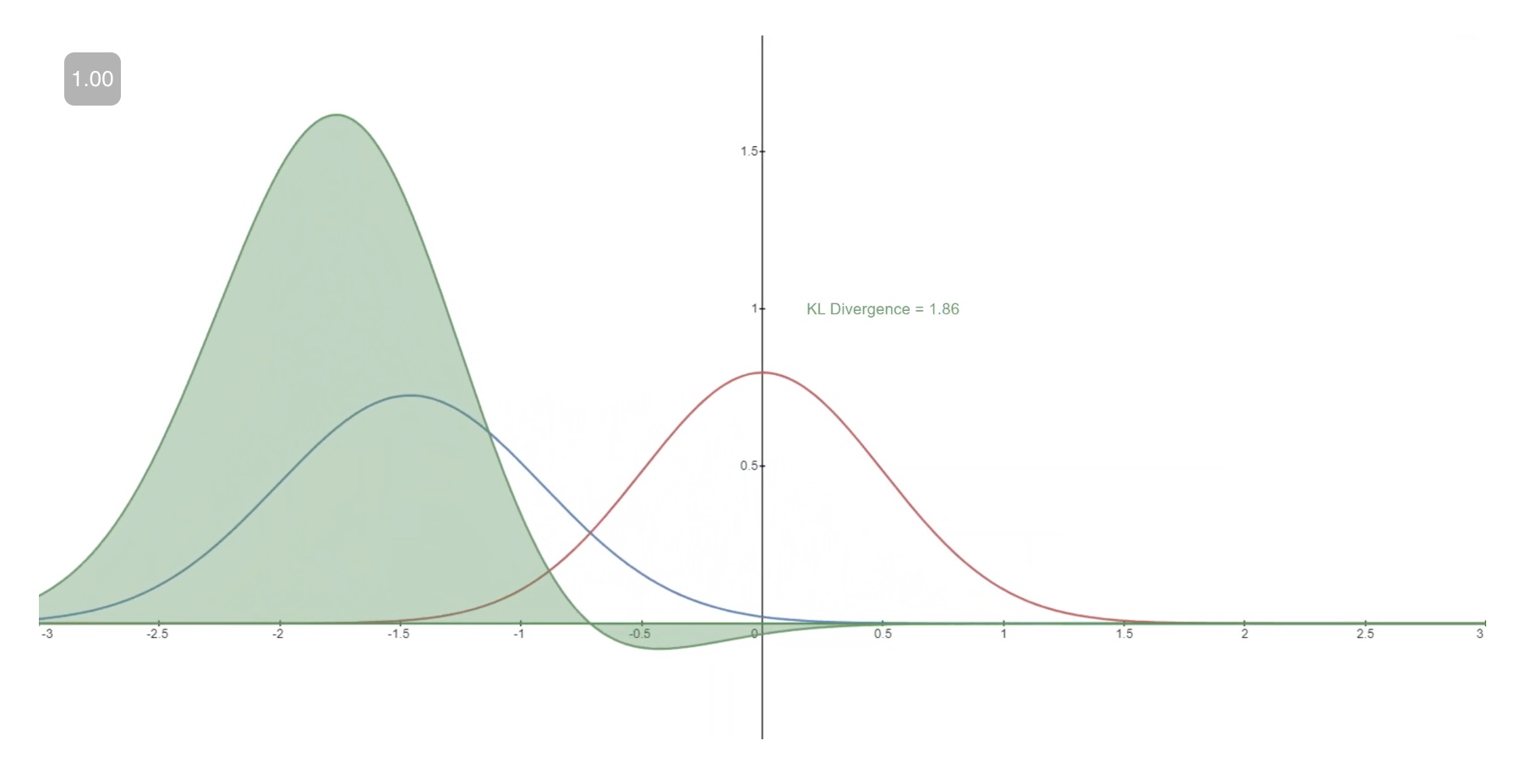
\[D_{\mathrm{KL}}(P \| Q)=\int_{-\infty}^{\infty} p(x) \log \left(\frac{p(x)}{q(x)}\right) d x\]- Note that the double bars in the above equation indicate that the function is not symmetric with respect to its arguments.
-
Below you can see the \(K L\) divergence of a varying distribution \(P\) (blue) from a reference distribution \(Q\) (red). The green curve indicates the function within the integral in the definition for the \(\mathrm{KL}\) divergence above, and the total area under the curve represents the value of the KL divergence of \(P\) from \(Q\) at any given moment, a value which is also displayed numerically.
Casting \(L_{v l b}\) in Terms of KL Divergences
-
As mentioned previously, it is possible[1] to rewrite \(L v l b\) almost completely in terms of KL divergences:
\[L_{v l b}=L_{0}+L_{1}+\ldots+L_{T-1}+L_{T}\]- where, \(\begin{gathered} L_{0}=-\log p_{\theta}\left(x_{0} \mid x_{1}\right) \\ L_{t-1}=D_{K L}\left(q\left(x_{t-1} \mid x_{t}, x_{0}\right) \| p_{\theta}\left(x_{t-1} \mid x_{t}\right)\right) \\ L_{T}=D_{K L}\left(q\left(x_{T} \mid x_{0}\right) \| p\left(x_{T}\right)\right) \end{gathered}\)
-
Conditioning the forward process posterior on \(x_{0}\) in \(L_{t-1}\) results in a tractable form that leads to all KL divergences being comparisons between Gaussians. This means that the divergences can be exactly calculated with closed-form expressions rather than with Monte Carlo estimates.
Model Choices
- With the mathematical foundation for our objective function established, we now need to make several choices regarding how our diffusion model will be implemented. For the forward process, the only choice required is defining the variance schedule, the values of which are generally increasing during the forward process.
- For the reverse process, we much choose the Gaussian distribution parameterization / model architecture(s). Note the high degree of flexibility that Diffusion models afford - the only requirement on our architecture is that its input and output have the same dimensionality. We will explore the details of these choices in more detail below.
Forward Process and \(L_{T}\)
- As noted above, regarding the forward process, we must define the variance schedule. In particular, we set them to be time-dependent constants, ignoring the fact that they can be learned. For example, per Denoising Diffusion Probabilistic models, a linear schedule from \(\beta_{1}=10^{-4}\) to \(\beta_{T}=0.2\) might be used, or perhaps a geometric series. Regardless of the particular values chosen, the fact that the variance schedule is fixed results in \(L_{T}\) becoming a constant with respect to our set of learnable parameters, allowing us to ignore it as far as training is concerned.
Reverse Process and \(L_{1: T-1}\)
- Now we discuss the choices required in defining the reverse process. Recall from above we defined the reverse Markov transitions as a Gaussian:
- We must now define the functional forms of \(\mu_{\theta}\) or \(\Sigma_{\theta}\). While there are more complicated ways to parameterize \(\boldsymbol{\Sigma}_\theta\), we simply set,
- That is, we assume that the multivariate Gaussian is a product of independent gaussians with identical variance, a variance value which can change with time. We set these variances to be equivalent to our forward process variance schedule.
-
Given this new formulation of \(\Sigma_{\theta_{1}}\), we have
\[p_{\theta}\left(\mathbf{x}_{t-1} \mid \mathbf{x}_{t}\right):=\mathcal{N}\left(\mathbf{x}_{t-1} ; \boldsymbol{\mu}_{\theta}\left(\mathbf{x}_{t}, t\right), \mathbf{\Sigma}_{\theta}\left(\mathbf{x}_{t}, t\right):=\mathcal{N}\left(\mathbf{x}_{t-1} ; \boldsymbol{\mu}_{\theta}\left(\mathbf{x}_{t}, t\right), \sigma_{t}^{2} \mathbf{I}\right)\right.\]- which allows us to transform,
- to,
- where the first term in the difference is a linear combination of \(x t\) and \(x_{0}\) that depends on the variance schedule \(\beta_{t}\). The exact form of this function is not relevant for our purposes, but it can be found in Denoising Diffusion Probabilistic models. The significance of the above proportion is that the most straightforward parameterization of \(\mu_{\theta}\) simply predicts the diffusion posterior mean. Importantly, the authors of Denoising Diffusion Probabilistic models actually found that training \(\mu \theta\) to predict the noise component at any given timestep yields better results. In particular, let
- where, \(\alpha_{t}:=1-\beta_{t} \quad\) and \(\quad \bar{\alpha}_{t}:=\prod_{s=1}^{t} \alpha_{s}\).
- This leads to the following alternative loss function, which the authors of Denoising Diffusion Probabilistic models found to lead to more stable training and better results:
- The authors of Denoising Diffusion Probabilistic models also note connections of this formulation of Diffusion models to score-matching generative models based on Langevin dynamics. Indeed, it appears that Diffusion models and ScoreBased models may be two sides of the same coin, akin to the independent and concurrent development of wave-based quantum mechanics and matrix-based quantum mechanics revealing two equivalent formulations of the same phenomena.
Network Architecture
- Lets dive deep into the network architecture of a diffusion model.
- Note that the only requirement for the model is that its input and output dimensionality are identical. Specifically, the neural network needs to take in a noised image at a particular time step and return the predicted noise. The predicted noise here is a tensor that has the same size and resolution as the input image. Thus, this neural networks takes in tensors and returns tensors of the same shape. Given this restriction, it is perhaps unsurprising that image diffusion models are commonly implemented with U-Net-like architectures.
- The neural net architecture that the authors of DDPM used was U-Net.
- This network consists of a “bottleneck” layer in the middle of its architecture in between the encoder and decoder.
- This bottleneck ensures the network learns only the most important information.
- The encoder first encodes an image into a smaller hidden representation called the “bottleneck” and then the decoder decodes that hidden representation back into an actual image.
- Below is a representation of the U-Net model:
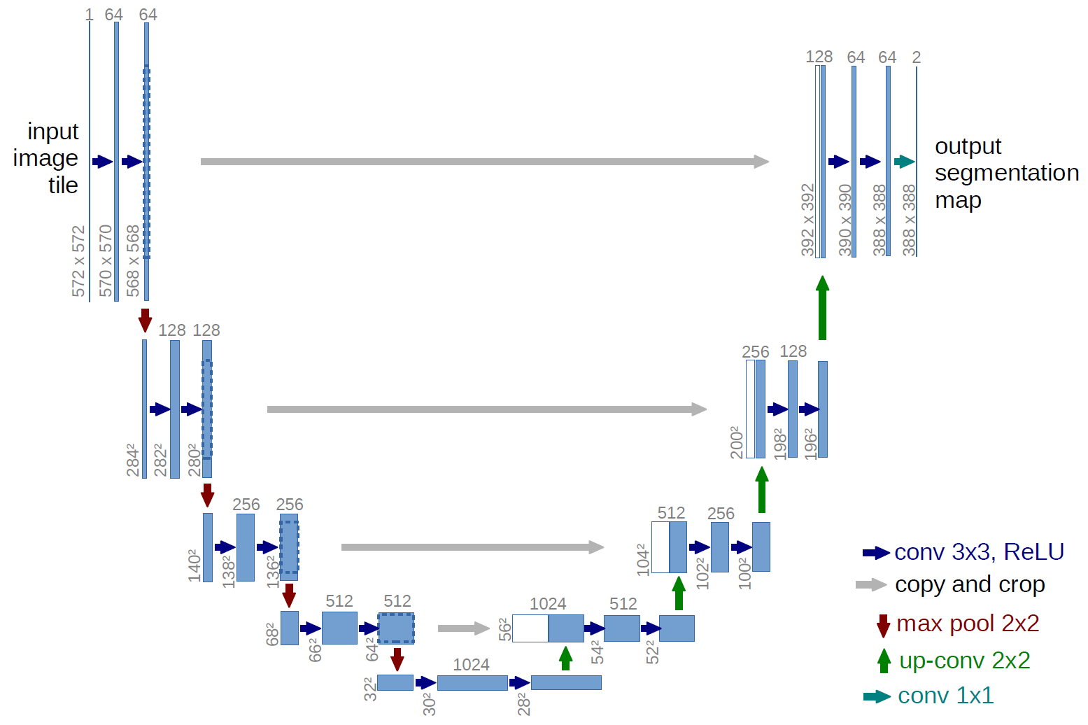
- The U-Net model first downsamples the input, or makes the input smaller in terms of spatial resolution, and then upsamples it.
Reverse Process Decoder and \(L_{0}\)
- The path along the reverse process consists of many transformations under continuous conditional Gaussian distributions. At the end of the reverse process, recall that we are trying to produce an image, which is composed of integer pixel values. Therefore, we must devise a way to obtain discrete (log) likelihoods for each possible pixel value across all pixels.
-
The way that this is done is by setting the last transition in the reverse diffusion chain to an independent discrete decoder. To determine the likelihood of a given image \(x 0\) given \(x 1_{1}\), we first impose independence between the data dimensions:
\[p_{\theta}\left(x_{0} \mid x_{1}\right)=\prod_{i=1}^{D} p_{\theta}\left(x_{0}^{i} \mid x_{1}^{i}\right)\]- where \(D\) is the dimensionality of the data and the superscript \(i\) indicates the extraction of one coordinate. The goal now is to determine how likely each integer value is for a given pixel given the distribution across possible values for the corresponding pixel in the slightly noised image at time \(t=1\) :
- where the pixel distributions for \(t=1\) are derived from the below multivariate Gaussian whose diagonal covariance matrix allows us to split the distribution into a product of univariate Gaussians, one for each dimension of the data:
-
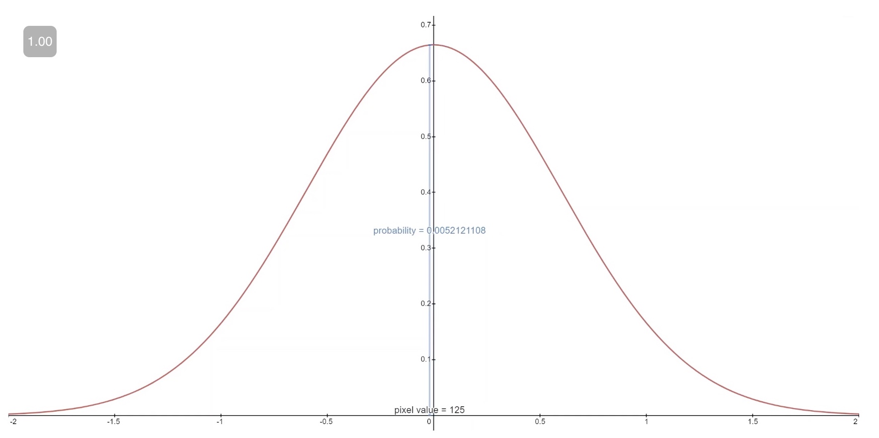
We assume that the images consist of integers in \(0,1, \ldots, 255\) (as standard RGB images do) which have been scaled linearly to \([-1,1]\). We then break down the real line into small “buckets”, where, for a given scaled pixel value \(x\), the bucket for that range is \([x-1 / 255, x+1 / 255]\). The probability of a pixel value \(x\), given the univariate Gaussian distribution of the corresponding pixel in \(x 1\), is the area under that univariate Gaussian distribution within the bucket centered at \(x\).
- Below you can see the area for each of these buckets with their probabilities for a mean-0 Gaussian which, in this context, corresponds to a distribution with an average pixel value of \(\frac{255}{2}\) (half brightness). The red curve represents the distribution of a specific pixel in the \(t=1\) image, and the areas give the probability of the corresponding pixel value in the \(t=0\) image.
-
Technical Note: The first and final buckets extend out to -inf and +inf to preserve total probability.
-
Given a \(t=0\) pixel value for each pixel, the value of \(p_{\theta}\left(x_{0} \mid x_{1}\right)\) is simply their product. Succinctly, this process is succinctly encapsulated by the following equation:
\[p_{\theta}\left(x_{0} \mid x_{1}\right)=\prod_{i=1}^{D} p_{\theta}\left(x_{0}^{i} \mid x_{1}^{i}\right)=\prod_{i=1}^{D} \int_{\delta_{-}\left(x_{0}^{i}\right)}^{\delta_{+}\left(x_{0}^{i}\right)} \mathcal{N}\left(x ; \mu_{\theta}^{i}\left(x_{1}, 1\right), \sigma_{1}^{2}\right) d x\]- where,
- and
-
Given this equation for \(p_{\theta}\left(x_{0} \mid x_{1}\right)\), we can calculate the final term of \(L_{v l b}\) which is not formulated as a \(\mathrm{KL}\) Divergence:
\[L_{0}=-\log p_{\theta}\left(x_{0} \mid x_{1}\right)\]
Final Objective
- As mentioned in the last section, the authors of Denoising Diffusion Probabilistic models found that predicting the noise component of an image at a given timestep produced the best results. Ultimately, they use the following objective:
- The training and sampling algorithms for our diffusion model therefore can be succinctly captured in the below table (from source):

Diffusion Model Theory Summary
-
In this section we took a detailed dive into the theory of Diffusion models. It can be easy to get caught up in mathematical details, so we note the most important points within this section below in order to keep ourselves oriented from a birds-eye perspective:
- Our diffusion model is parameterized as a Markov chain, meaning that our latent variables \(x_1, \ldots, x_T\) depend only on the previous (or following) timestep.
- The transition distributions in the Markov chain are Gaussian, where the forward process requires a variance schedule, and the reverse process parameters are learned.
- The diffusion process ensures that \(x T\) is asymptotically distributed as an isotropic Gaussian for sufficiently large \(\mathrm{T}\).
- In our case, the variance schedule was fixed, but it can be learned as well. For fixed schedules, following a geometric progression may afford better results than a linear progression. In either case, the variances are generally increasing with time in the series (i.e. \(\beta_{i}<\beta_{j}\) for \(i<j\) ).
- Diffusion models are highly flexible and allow for any architecture whose input and output dimensionality are the same to be used. Many implementations use U-Net-like architectures.
- The training objective is to maximize the likelihood of the training data. This is manifested as tuning the model parameters to minimize the variational upper bound of the negative log likelihood of the data.
- Almost all terms in the objective function can be cast as KL Divergences as a result of our Markov assumption. These values become tenable to calculate given that we are using Gaussians, therefore omitting the need to perform Monte Carlo approximation.
- Ultimately, using a simplified training objective to train a function which predicts the noise component of a given latent variable yields the best and most stable results.
- A discrete decoder is used to obtain log likelihoods across pixel values as the last step in the reverse diffusion process.
-
With this high-level overview of Diffusion models in our minds, let’s move on to see how to use a Diffusion models in PyTorch.
Diffusion models in PyTorch 👩🏽💻
Implementing the original paper
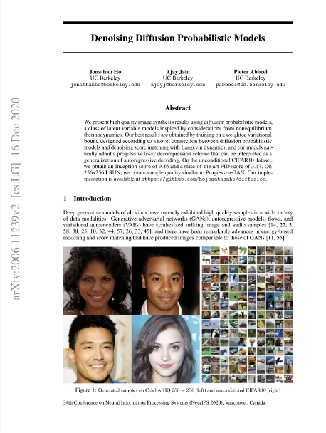
- Let’s go over the original Denoising Diffusion Probabilistic Models (DDPMs) paper by Ho et al.,2020 and implement it step by step based on Phil Wang’s implementation and The Annotated Diffusion by Hugging Face which are both based off the original implementation.
Pre-requisites: Setup and Importing Libraries
- Let’s start with the setup and importing all the required libraries:
from IPython.display import Image
Image(filename='assets/78_annotated-diffusion/ddpm_paper.png')

!pip install -q -U einops datasets matplotlib tqdm

import math
from inspect import isfunction
from functools import partial

%matplotlib inline
import matplotlib.pyplot as plt
from tqdm.auto import tqdm
from einops import rearrange

import torch
from torch import nn, einsum
import torch.nn.functional as F
Helper functions
- Now let’s implement the neural network we have looked at earlier. First we start with a few helper functions.
- Most notably, we define
Residualclass which will add the input to the output of a particular function. That is, it adds a residual connection to a particular function.
def exists(x):
    return x is not None

def default(val, d):
    if exists(val):
        return val
    return d() if isfunction(d) else d

class Residual(nn.Module):
    def __init__(self, fn):
        super().__init__()
        self.fn = fn

    def forward(self, x, *args, **kwargs):
        return self.fn(x, *args, **kwargs) + x

def Upsample(dim):
    return nn.ConvTranspose2d(dim, dim, 4, 2, 1)

def Downsample(dim):
    return nn.Conv2d(dim, dim, 4, 2, 1)
- Note: the parameters of the neural network are shared across time (noise level).
- Thus, for the neural network to keep track of which time step (noise level) it is on, the authors used sinusoidal position embeddings to encode \(t\).
- The
SinusoidalPositionEmbeddingsclass, that we have defined below, takes a tensor of shape(batch_size,1)as input or the noise levels in a batch. - It will then turn this input tensor into a tensor of shape
(batch_size, dim)wheredim$is the dimensionality of the position embeddings.
class SinusoidalPositionEmbeddings(nn.Module):
    def __init__(self, dim):
        super().__init__()
        self.dim = dim

    def forward(self, time):
        device = time.device
        half_dim = self.dim // 2
        embeddings = math.log(10000) / (half_dim - 1)
        embeddings = torch.exp(torch.arange(half_dim, device=device) * -embeddings)
        embeddings = time[:, None] * embeddings[None, :]
        embeddings = torch.cat((embeddings.sin(), embeddings.cos()), dim=-1)
        return embeddings
Model Core: ResNet or ConvNeXT
- Now we will look at the meat or the core part of our U-Net model. The original DDPM authors employed a Wide ResNet block via Zagoruyko et al., 2016, however Phil Wang has also introduced support for ConvNeXT block via Liu et al., 2022.
- You are free to choose either or in your final U-Net architecture but both are provided below:
class Block(nn.Module):
    def __init__(self, dim, dim_out, groups = 8):
        super().__init__()
        self.proj = nn.Conv2d(dim, dim_out, 3, padding = 1)
        self.norm = nn.GroupNorm(groups, dim_out)
        self.act = nn.SiLU()

    def forward(self, x, scale_shift = None):
        x = self.proj(x)
        x = self.norm(x)

        if exists(scale_shift):
            scale, shift = scale_shift
            x = x * (scale + 1) + shift

        x = self.act(x)
        return x

class ResnetBlock(nn.Module):
    """https://arxiv.org/abs/1512.03385"""

    def __init__(self, dim, dim_out, *, time_emb_dim=None, groups=8):
        super().__init__()
        self.mlp = (
            nn.Sequential(nn.SiLU(), nn.Linear(time_emb_dim, dim_out))
            if exists(time_emb_dim)
            else None
        )

        self.block1 = Block(dim, dim_out, groups=groups)
        self.block2 = Block(dim_out, dim_out, groups=groups)
        self.res_conv = nn.Conv2d(dim, dim_out, 1) if dim != dim_out else nn.Identity()

    def forward(self, x, time_emb=None):
        h = self.block1(x)

        if exists(self.mlp) and exists(time_emb):
            time_emb = self.mlp(time_emb)
            h = rearrange(time_emb, "b c -> b c 1 1") + h

        h = self.block2(h)
        return h + self.res_conv(x)

class ConvNextBlock(nn.Module):
    """https://arxiv.org/abs/2201.03545"""

    def __init__(self, dim, dim_out, *, time_emb_dim=None, mult=2, norm=True):
        super().__init__()
        self.mlp = (
            nn.Sequential(nn.GELU(), nn.Linear(time_emb_dim, dim))
            if exists(time_emb_dim)
            else None
        )

        self.ds_conv = nn.Conv2d(dim, dim, 7, padding=3, groups=dim)

        self.net = nn.Sequential(
            nn.GroupNorm(1, dim) if norm else nn.Identity(),
            nn.Conv2d(dim, dim_out * mult, 3, padding=1),
            nn.GELU(),
            nn.GroupNorm(1, dim_out * mult),
            nn.Conv2d(dim_out * mult, dim_out, 3, padding=1),
        )

        self.res_conv = nn.Conv2d(dim, dim_out, 1) if dim != dim_out else nn.Identity()

    def forward(self, x, time_emb=None):
        h = self.ds_conv(x)

        if exists(self.mlp) and exists(time_emb):
            condition = self.mlp(time_emb)
            h = h + rearrange(condition, "b c -> b c 1 1")

        h = self.net(h)
        return h + self.res_conv(x)
Attention
- Next, we will look into defining the attention module which was added between the convolutional blocks in DDPM.
- Phil Wang added two variants of attention, a normal multi-headed self-attention from the original Transformer paper (Vaswani et al.,2017), and linear attention variant (Shen et al., 2018).
- Linear attention variant’s time and memory requirements scale linear in the sequence length, as opposed to quadratic for regular attention.
class Attention(nn.Module):
    def __init__(self, dim, heads=4, dim_head=32):
        super().__init__()
        self.scale = dim_head**-0.5
        self.heads = heads
        hidden_dim = dim_head * heads
        self.to_qkv = nn.Conv2d(dim, hidden_dim * 3, 1, bias=False)
        self.to_out = nn.Conv2d(hidden_dim, dim, 1)

    def forward(self, x):
        b, c, h, w = x.shape
        qkv = self.to_qkv(x).chunk(3, dim=1)
        q, k, v = map(
            lambda t: rearrange(t, "b (h c) x y -> b h c (x y)", h=self.heads), qkv
        )
        q = q * self.scale

        sim = einsum("b h d i, b h d j -> b h i j", q, k)
        sim = sim - sim.amax(dim=-1, keepdim=True).detach()
        attn = sim.softmax(dim=-1)

        out = einsum("b h i j, b h d j -> b h i d", attn, v)
        out = rearrange(out, "b h (x y) d -> b (h d) x y", x=h, y=w)
        return self.to_out(out)

class LinearAttention(nn.Module):
    def __init__(self, dim, heads=4, dim_head=32):
        super().__init__()
        self.scale = dim_head**-0.5
        self.heads = heads
        hidden_dim = dim_head * heads
        self.to_qkv = nn.Conv2d(dim, hidden_dim * 3, 1, bias=False)

        self.to_out = nn.Sequential(nn.Conv2d(hidden_dim, dim, 1),
                                    nn.GroupNorm(1, dim))

    def forward(self, x):
        b, c, h, w = x.shape
        qkv = self.to_qkv(x).chunk(3, dim=1)
        q, k, v = map(
            lambda t: rearrange(t, "b (h c) x y -> b h c (x y)", h=self.heads), qkv
        )

        q = q.softmax(dim=-2)
        k = k.softmax(dim=-1)

        q = q * self.scale
        context = torch.einsum("b h d n, b h e n -> b h d e", k, v)

        out = torch.einsum("b h d e, b h d n -> b h e n", context, q)
        out = rearrange(out, "b h c (x y) -> b (h c) x y", h=self.heads, x=h, y=w)
        return self.to_out(out)
- DDPM then adds group normalization to interleave the convolutional/attention layers of the U-Net architecture.
- Below, the
PreNormclass will apply group normalization before the attention layer.- Note, there has been a debate about whether groupnorm is better to be applied before or after attention in Transformers.
class PreNorm(nn.Module):
    def __init__(self, dim, fn):
        super().__init__()
        self.fn = fn
        self.norm = nn.GroupNorm(1, dim)

    def forward(self, x):
        x = self.norm(x)
        return self.fn(x)
Overall network
- Now that we have all the building blocks of the neural network (ResNet/ConvNeXT blocks, attention, positional embeddings, group norm), lets define our entire neural network.
- The task of this neural network is to take in a batch of noisy images and their noise levels and then to output the noise added to the input.
- The network takes a batch of noisy images of shape
(batch_size, num_channels, height, width)and a batch of noise levels of shape(batch_size, 1)as input, and returns a tensor of shape(batch_size, num_channels, height, width). - The network is built up as follows: (source)
- first, a convolutional layer is applied on the batch of noisy images, and position embeddings are computed for the noise levels
- next, a sequence of downsampling stages are applied.
- Each downsampling stage consists of two ResNet/ConvNeXT blocks + groupnorm + attention + residual connection + a downsample operation
- at the middle of the network, again ResNet or ConvNeXT blocks are applied, interleaved with attention
- next, a sequence of upsampling stages are applied.
- Each upsampling stage consists of two ResNet/ConvNeXT blocks + groupnorm + attention + residual connection + an upsample operation
- finally, a ResNet/ConvNeXT block followed by a convolutional layer is applied.
class Unet(nn.Module):
    def __init__(
        self,
        dim,
        init_dim=None,
        out_dim=None,
        dim_mults=(1, 2, 4, 8),
        channels=3,
        with_time_emb=True,
        resnet_block_groups=8,
        use_convnext=True,
        convnext_mult=2,
    ):
        super().__init__()

        # determine dimensions
        self.channels = channels

        init_dim = default(init_dim, dim // 3 * 2)
        self.init_conv = nn.Conv2d(channels, init_dim, 7, padding=3)

        dims = [init_dim, *map(lambda m: dim * m, dim_mults)]
        in_out = list(zip(dims[:-1], dims[1:]))

        if use_convnext:
            block_klass = partial(ConvNextBlock, mult=convnext_mult)
        else:
            block_klass = partial(ResnetBlock, groups=resnet_block_groups)

        # time embeddings
        if with_time_emb:
            time_dim = dim * 4
            self.time_mlp = nn.Sequential(
                SinusoidalPositionEmbeddings(dim),
                nn.Linear(dim, time_dim),
                nn.GELU(),
                nn.Linear(time_dim, time_dim),
            )
        else:
            time_dim = None
            self.time_mlp = None

        # layers
        self.downs = nn.ModuleList([])
        self.ups = nn.ModuleList([])
        num_resolutions = len(in_out)

        for ind, (dim_in, dim_out) in enumerate(in_out):
            is_last = ind >= (num_resolutions - 1)

            self.downs.append(
                nn.ModuleList(
                    [
                        block_klass(dim_in, dim_out, time_emb_dim=time_dim),
                        block_klass(dim_out, dim_out, time_emb_dim=time_dim),
                        Residual(PreNorm(dim_out, LinearAttention(dim_out))),
                        Downsample(dim_out) if not is_last else nn.Identity(),
                    ]
                )
            )

        mid_dim = dims[-1]
        self.mid_block1 = block_klass(mid_dim, mid_dim, time_emb_dim=time_dim)
        self.mid_attn = Residual(PreNorm(mid_dim, Attention(mid_dim)))
        self.mid_block2 = block_klass(mid_dim, mid_dim, time_emb_dim=time_dim)

        for ind, (dim_in, dim_out) in enumerate(reversed(in_out[1:])):
            is_last = ind >= (num_resolutions - 1)

            self.ups.append(
                nn.ModuleList(
                    [
                        block_klass(dim_out * 2, dim_in, time_emb_dim=time_dim),
                        block_klass(dim_in, dim_in, time_emb_dim=time_dim),
                        Residual(PreNorm(dim_in, LinearAttention(dim_in))),
                        Upsample(dim_in) if not is_last else nn.Identity(),
                    ]
                )
            )

        out_dim = default(out_dim, channels)
        self.final_conv = nn.Sequential(
            block_klass(dim, dim), nn.Conv2d(dim, out_dim, 1)
        )

    def forward(self, x, time):
        x = self.init_conv(x)

        t = self.time_mlp(time) if exists(self.time_mlp) else None

        h = []

        # downsample
        for block1, block2, attn, downsample in self.downs:
            x = block1(x, t)
            x = block2(x, t)
            x = attn(x)
            h.append(x)
            x = downsample(x)

        # bottleneck
        x = self.mid_block1(x, t)
        x = self.mid_attn(x)
        x = self.mid_block2(x, t)

        # upsample
        for block1, block2, attn, upsample in self.ups:
            x = torch.cat((x, h.pop()), dim=1)
            x = block1(x, t)
            x = block2(x, t)
            x = attn(x)
            x = upsample(x)

        return self.final_conv(x)
- Note: by default, the noise predictor uses ConvNeXT blocks (as
use_convnextis set to True) and position embeddings are added (aswith_time_embis set to True).
Forward diffusion
- Now lets take a look at the forward diffusion process. Remember forward diffusion process will gradually add noise to an image withing a number of time steps \(T\).
def cosine_beta_schedule(timesteps, s=0.008):
    """
    cosine schedule as proposed in https://arxiv.org/abs/2102.09672
    """
    steps = timesteps + 1
    x = torch.linspace(0, timesteps, steps)
    alphas_cumprod = torch.cos(((x / timesteps) + s) / (1 + s) * torch.pi * 0.5) ** 2
    alphas_cumprod = alphas_cumprod / alphas_cumprod[0]
    betas = 1 - (alphas_cumprod[1:] / alphas_cumprod[:-1])
    return torch.clip(betas, 0.0001, 0.9999)

def linear_beta_schedule(timesteps):
    beta_start = 0.0001
    beta_end = 0.02
    return torch.linspace(beta_start, beta_end, timesteps)

def quadratic_beta_schedule(timesteps):
    beta_start = 0.0001
    beta_end = 0.02
    return torch.linspace(beta_start**0.5, beta_end**0.5, timesteps) ** 2

def sigmoid_beta_schedule(timesteps):
    beta_start = 0.0001
    beta_end = 0.02
    betas = torch.linspace(-6, 6, timesteps)
    return torch.sigmoid(betas) * (beta_end - beta_start) + beta_start
- To start with, let’s use the linear schedule for T=200T time steps and define the various variables from the \(\beta_t\) which we will need, such as the cumulative product of the variances \(\bar{\alpha}_t\)
- Each of the variables below are just 1-dimensional tensors, storing values from \(t\) to \(T\).
- Importantly, we also define an extract function, which will allow us to extract the appropriate tt index for a batch of indices. (source)
timesteps = 200

# define beta schedule
betas = linear_beta_schedule(timesteps=timesteps)

# define alphas
alphas = 1. - betas
alphas_cumprod = torch.cumprod(alphas, axis=0)
alphas_cumprod_prev = F.pad(alphas_cumprod[:-1], (1, 0), value=1.0)
sqrt_recip_alphas = torch.sqrt(1.0 / alphas)

# calculations for diffusion q(x_t | x_{t-1}) and others
sqrt_alphas_cumprod = torch.sqrt(alphas_cumprod)
sqrt_one_minus_alphas_cumprod = torch.sqrt(1. - alphas_cumprod)

# calculations for posterior q(x_{t-1} | x_t, x_0)
posterior_variance = betas * (1. - alphas_cumprod_prev) / (1. - alphas_cumprod)

def extract(a, t, x_shape):
    batch_size = t.shape[0]
    out = a.gather(-1, t.cpu())
    return out.reshape(batch_size, *((1,) * (len(x_shape) - 1))).to(t.device)
- Now let’s take an image and illustrate how noise is added at each time step of the diffusion process to the PyTorch tensors:
from PIL import Image
import requests

url = 'http://images.cocodataset.org/val2017/000000039769.jpg'
image = Image.open(requests.get(url, stream=True).raw)
image
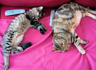
- We first normalize images by dividing by 255 (such that they are in the
[0,1]range), and then make sure they are in the[-1, 1]range.
from torchvision.transforms import Compose, ToTensor, Lambda, ToPILImage, CenterCrop, Resize

image_size = 128
transform = Compose([
    Resize(image_size),
    CenterCrop(image_size),
    ToTensor(), # turn into Numpy array of shape HWC, divide by 255
    Lambda(lambda t: (t * 2) - 1),

])

x_start = transform(image).unsqueeze(0)
x_start.shape
Output:
----------------------------------------------------------------------------------------------------
torch.Size([1, 3, 128, 128])
- We also define the reverse transform, which takes in a PyTorch tensor containing values in
[-1, 1]and turn them back into a PIL image:
import numpy as np

reverse_transform = Compose([
     Lambda(lambda t: (t + 1) / 2),
     Lambda(lambda t: t.permute(1, 2, 0)), # CHW to HWC
     Lambda(lambda t: t * 255.),
     Lambda(lambda t: t.numpy().astype(np.uint8)),
     ToPILImage(),
])
- Let’s run an example and see what it produces:
reverse_transform(x_start.squeeze())

- We can now define the forward diffusion process as in the paper:
# forward diffusion (using the nice property)
def q_sample(x_start, t, noise=None):
    if noise is None:
        noise = torch.randn_like(x_start)

    sqrt_alphas_cumprod_t = extract(sqrt_alphas_cumprod, t, x_start.shape)
    sqrt_one_minus_alphas_cumprod_t = extract(
        sqrt_one_minus_alphas_cumprod, t, x_start.shape
    )

    return sqrt_alphas_cumprod_t * x_start + sqrt_one_minus_alphas_cumprod_t * noise
- Let’s test it on a particular time step and see the image it produces:
def get_noisy_image(x_start, t):
  # add noise
  x_noisy = q_sample(x_start, t=t)

  # turn back into PIL image
  noisy_image = reverse_transform(x_noisy.squeeze())

  return noisy_image
# take time step
t = torch.tensor([40])

get_noisy_image(x_start, t)

- We can see the image is getting more noisy. Now let’s zoom out a bit and visualize this for various time steps:
import matplotlib.pyplot as plt

# use seed for reproducability
torch.manual_seed(0)

# source: https://pytorch.org/vision/stable/auto_examples/plot_transforms.html#sphx-glr-auto-examples-plot-transforms-py
def plot(imgs, with_orig=False, row_title=None, **imshow_kwargs):
    if not isinstance(imgs[0], list):
        # Make a 2d grid even if there's just 1 row
        imgs = [imgs]

    num_rows = len(imgs)
    num_cols = len(imgs[0]) + with_orig
    fig, axs = plt.subplots(figsize=(200,200), nrows=num_rows, ncols=num_cols, squeeze=False)
    for row_idx, row in enumerate(imgs):
        row = [image] + row if with_orig else row
        for col_idx, img in enumerate(row):
            ax = axs[row_idx, col_idx]
            ax.imshow(np.asarray(img), **imshow_kwargs)
            ax.set(xticklabels=[], yticklabels=[], xticks=[], yticks=[])

    if with_orig:
        axs[0, 0].set(title='Original image')
        axs[0, 0].title.set_size(8)
    if row_title is not None:
        for row_idx in range(num_rows):
            axs[row_idx, 0].set(ylabel=row_title[row_idx])

    plt.tight_layout()
plot([get_noisy_image(x_start, torch.tensor([t])) for t in [0, 50, 100, 150, 199]])

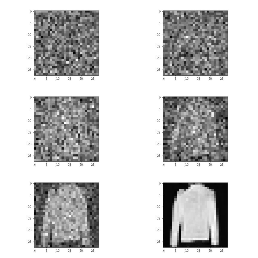
- As we can see above, the image going through forward diffusion is definitely becoming more apparent.
- Thus, we can now move on to defining our loss function. The
denoise_modelwill be our U-Net defined above. We’ll employ the Huber loss between the true and the predicted noise.
def p_losses(denoise_model, x_start, t, noise=None, loss_type="l1"):
    if noise is None:
        noise = torch.randn_like(x_start)

    x_noisy = q_sample(x_start=x_start, t=t, noise=noise)
    predicted_noise = denoise_model(x_noisy, t)

    if loss_type == 'l1':
        loss = F.l1_loss(noise, predicted_noise)
    elif loss_type == 'l2':
        loss = F.mse_loss(noise, predicted_noise)
    elif loss_type == "huber":
        loss = F.smooth_l1_loss(noise, predicted_noise)
    else:
        raise NotImplementedError()

    return loss
Dataset
- Let’s now look into loading up our dataset. A quick note, our dataset needs to make sure all images are resized to the same size.
- Hugging Face’s fashion_mnist dataset which we will use in this example already does that for us with all images having a same resolution of \(28 \times 28\).
from datasets import load_dataset

# load dataset from the hub
dataset = load_dataset("fashion_mnist")
image_size = 28
channels = 1
batch_size = 128
- Now, we will define a function
transformswhich we’ll apply on-the-fly on the entire dataset. - The function just applies some basic image preprocessing: random horizontal flips, rescaling and finally make them have values in the
[-1,1]range.
from torchvision import transforms
from torch.utils.data import DataLoader

# define image transformations (e.g. using torchvision)
transform = Compose([
            transforms.RandomHorizontalFlip(),
            transforms.ToTensor(),
            transforms.Lambda(lambda t: (t * 2) - 1)
])

# define function
def transforms(examples):
   examples["pixel_values"] = [transform(image.convert("L")) for image in examples["image"]]
   del examples["image"]

   return examples

transformed_dataset = dataset.with_transform(transforms).remove_columns("label")

# create dataloader
dataloader = DataLoader(transformed_dataset["train"], batch_size=batch_size, shuffle=True)
batch = next(iter(dataloader))
print(batch.keys())
Output:
----------------------------------------------------------------------------------------------------
dict_keys(['pixel_values'])
Sampling during training
- The paper also talks about sampling from the model during training in order to track progress.
- Ideally, generating new images from a diffusion model happens by reversing the diffusion process:
- We start from \(T\), where we sample pure noise from a Gaussian distribution
- Then use our neural network to gradually de-noise it using the conditional probability it has learned, continuing until we end up at time step \(t\) = 0.
- We can derive a slightly less de-noised image \(x_{(t-1)}\) by plugging in the re-parametrization of the mean, using our noise predictor.
- Remember that the variance is known ahead of time.
- After all of this, ideally, we end up with an image that looks like it came from the real data distribution.
- Lets look at the code for that below:
@torch.no_grad()
def p_sample(model, x, t, t_index):
    betas_t = extract(betas, t, x.shape)
    sqrt_one_minus_alphas_cumprod_t = extract(
        sqrt_one_minus_alphas_cumprod, t, x.shape
    )
    sqrt_recip_alphas_t = extract(sqrt_recip_alphas, t, x.shape)

    # Equation 11 in the paper
    # Use our model (noise predictor) to predict the mean
    model_mean = sqrt_recip_alphas_t * (
        x - betas_t * model(x, t) / sqrt_one_minus_alphas_cumprod_t
    )

    if t_index == 0:
        return model_mean
    else:
        posterior_variance_t = extract(posterior_variance, t, x.shape)
        noise = torch.randn_like(x)
        # Algorithm 2 line 4:
        return model_mean + torch.sqrt(posterior_variance_t) * noise

# Algorithm 2 (including returning all images)
@torch.no_grad()
def p_sample_loop(model, shape):
    device = next(model.parameters()).device

    b = shape[0]
    # start from pure noise (for each example in the batch)
    img = torch.randn(shape, device=device)
    imgs = []

    for i in tqdm(reversed(range(0, timesteps)), desc='sampling loop time step', total=timesteps):
        img = p_sample(model, img, torch.full((b,), i, device=device, dtype=torch.long), i)
        imgs.append(img.cpu().numpy())
    return imgs

@torch.no_grad()
def sample(model, image_size, batch_size=16, channels=3):
    return p_sample_loop(model, shape=(batch_size, channels, image_size, image_size))
- Now, lets get to some training! We will train the model via PyTorch and occasionally save a few image samples using the
samplefunction from above.
from pathlib import Path

def num_to_groups(num, divisor):
    groups = num // divisor
    remainder = num % divisor
    arr = [divisor] * groups
    if remainder > 0:
        arr.append(remainder)
    return arr

results_folder = Path("./results")
results_folder.mkdir(exist_ok = True)
save_and_sample_every = 1000
- Below, we define the model, and move it to the GPU along with defining Adam, a standard optimizer.
from torch.optim import Adam

device = "cuda" if torch.cuda.is_available() else "cpu"

model = Unet(
    dim=image_size,
    channels=channels,
    dim_mults=(1, 2, 4,)
)
model.to(device)

optimizer = Adam(model.parameters(), lr=1e-3)
Training
- Now lets start the training process:
from torchvision.utils import save_image

epochs = 5

for epoch in range(epochs):
    for step, batch in enumerate(dataloader):
      optimizer.zero_grad()

      batch_size = batch["pixel_values"].shape[0]
      batch = batch["pixel_values"].to(device)

      # Algorithm 1 line 3: sample t uniformally for every example in the batch
      t = torch.randint(0, timesteps, (batch_size,), device=device).long()

      loss = p_losses(model, batch, t, loss_type="huber")

      if step % 100 == 0:
        print("Loss:", loss.item())

      loss.backward()
      optimizer.step()

      # save generated images
      if step != 0 and step % save_and_sample_every == 0:
        milestone = step // save_and_sample_every
        batches = num_to_groups(4, batch_size)
        all_images_list = list(map(lambda n: sample(model, batch_size=n, channels=channels), batches))
        all_images = torch.cat(all_images_list, dim=0)
        all_images = (all_images + 1) * 0.5
        save_image(all_images, str(results_folder / f'sample-{milestone}.png'), nrow = 6)
Output:
----------------------------------------------------------------------------------------------------
Loss: 0.46477368474006653
Loss: 0.12143351882696152
Loss: 0.08106148988008499
Loss: 0.0801810547709465
Loss: 0.06122320517897606
Loss: 0.06310459971427917
Loss: 0.05681884288787842
Loss: 0.05729678273200989
Loss: 0.05497899278998375
Loss: 0.04439849033951759
Loss: 0.05415581166744232
Loss: 0.06020551547408104
Loss: 0.046830907464027405
Loss: 0.051029372960329056
Loss: 0.0478244312107563
Loss: 0.046767622232437134
Loss: 0.04305662214756012
Loss: 0.05216279625892639
Loss: 0.04748568311333656
Loss: 0.05107741802930832
Loss: 0.04588869959115982
Loss: 0.043014321476221085
Loss: 0.046371955424547195
Loss: 0.04952816292643547
Loss: 0.04472338408231735
- And finally, let’s look at our inference or sampling from the
samplefunction we defined above.
# sample 64 images
samples = sample(model, image_size=image_size, batch_size=64, channels=channels)

# show a random one
random_index = 5
plt.imshow(samples[-1][random_index].reshape(image_size, image_size, channels), cmap="gray")

- Seems like the model is capable of generating a nice T-shirt! Keep in mind that the dataset we trained on is pretty low-resolution (28x28).
Creating a GIF
- Lastly, in order to see the progression of the de-noising process, we can create a GIF:
import matplotlib.animation as animation

random_index = 53

fig = plt.figure()
ims = []
for i in range(timesteps):
    im = plt.imshow(samples[i][random_index].reshape(image_size, image_size, channels), cmap="gray", animated=True)
    ims.append([im])

animate = animation.ArtistAnimation(fig, ims, interval=50, blit=True, repeat_delay=1000)
animate.save('diffusion.gif')
plt.show()
- Hopefully this was beneficial in clarifying the diffusion model concepts!
- Furthermore, it his highly recommend looking at Hugging Face’s Training with Diffusers notebook to see how to leverage their Diffusion library to train a simple model.
- And, for inference, they also provide this notebook where you can see the images being generated.
denoising-diffusion-pytorch package
- While Diffusion models have not yet been democratized to the same degree as other older architectures/approaches in Machine Learning, there are still implementations available for use. The easiest way to use a diffusion model in PyTorch is to use the
denoising-diffusion-pytorchpackage, which implements an image diffusion model like the one discussed in this article. To install the package, simply type the following command in the terminal:
pip install denoising_diffusion_pytorch
Minimal Example
- To train a model and generate images, we first import the necessary packages:
import torch
from denoising_diffusion_pytorch import Unet, GaussianDiffusion
- Next, we define our network architecture, in this case a U-Net. The
dimparameter specifies the number of feature maps before the first down-sampling, and thedim_multsparameter provides multiplicands for this value and successive down-samplings:
model = Unet(
    dim = 64,
    dim_mults = (1, 2, 4, 8)
)
- Now that our network architecture is defined, we need to define the diffusion model itself. We pass in the U-Net model that we just defined along with several parameters - the size of images to generate, the number of timesteps in the diffusion process, and a choice between the L1 and L2 norms.
diffusion = GaussianDiffusion(
    model,
    image_size = 128,
    timesteps = 1000,   # number of steps
    loss_type = 'l1'    # L1 or L2
)
- Now that the diffusion model is defined, it’s time to train. We generate random data to train on, and then train the diffusion model in the usual fashion:
training_images = torch.randn(8, 3, 128, 128)
loss = diffusion(training_images)
loss.backward()
- Once the model is trained, we can finally generate images by using the
sample()method of thediffusionobject. Here we generate 4 images, which are only noise given that our training data was random:
sampled_images = diffusion.sample(batch_size = 4)

Training on Custom Data
- The
denoising-diffusion-pytorchpackage also allow you to train a diffusion model on a specific dataset. Simply replace the'path/to/your/images'string with the dataset directory path in theTrainer()object below, and changeimage_sizeto the appropriate value. After that, simply run the code to train the model, and then sample as before. Note that PyTorch must be compiled with CUDA enabled in order to use theTrainerclass:
from denoising_diffusion_pytorch import Unet, GaussianDiffusion, Trainer

model = Unet(
    dim = 64,
    dim_mults = (1, 2, 4, 8)
).cuda()

diffusion = GaussianDiffusion(
    model,
    image_size = 128,
    timesteps = 1000,   # number of steps
    loss_type = 'l1'    # L1 or L2
).cuda()

trainer = Trainer(
    diffusion,
    'path/to/your/images',
    train_batch_size = 32,
    train_lr = 2e-5,
    train_num_steps = 700000,         # total training steps
    gradient_accumulate_every = 2,    # gradient accumulation steps
    ema_decay = 0.995,                # exponential moving average decay
    amp = True                        # turn on mixed precision
)

trainer.train()
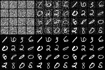
- Below you can see progressive denoising from multivariate Gaussian noise to MNIST digits akin to reverse diffusion:
HuggingFace Diffusers
- HuggingFace diffusers provides pretrained diffusion models across multiple modalities, such as vision and audio, and serves as a modular toolbox for inference and training of diffusion models.

- More precisely, HuggingFace Diffusers offers:
- State-of-the-art diffusion pipelines that can be run in inference with just a couple of lines of code.
- Various noise schedulers that can be used interchangeably for the prefered speed vs. quality trade-off in inference.
- Multiple types of models, such as UNet, that can be used as building blocks in an end-to-end diffusion system.
- Training examples to show how to train the most popular diffusion models.
Implementations
Stable Diffusion
- Stable Diffusion is a state of the art text-to-image model that generates images from text. It’s makes it’s high performance models available to the public at large to use here.
- Stable Diffusion is a text-to-image latent diffusion model created by the researchers and engineers from CompVis, Stability AI and LAION. It is trained on 512x512 images from a subset of the LAION-5B database which is the largest, freely accessible multi-modal dataset. (source)
- Let’s now look at how it works with the illustrations below by Jay Alammar.
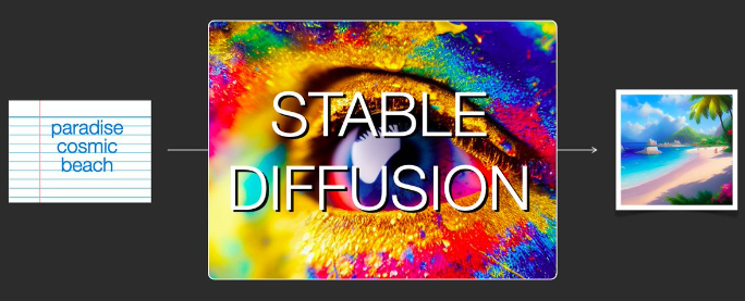
- Stable Diffusion is quite versatile because it can be used in a variety of ways.
- In the image we see above, we can see that it can take text as input and output a generated image. This is the primary use case, however, it is not the only one.
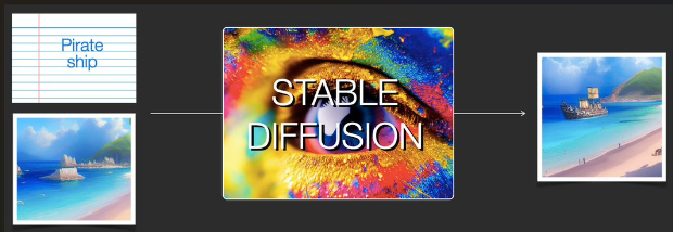
- As we can see from the image above, another use case of Stable Diffusion is with image and text as input, and it will output a generated image again. This is called img2img.
- It’s able to be so versatile because Stable Diffusion is not one monolith model, but a system made up of several components and models.
- To be specific, Stable Diffusion is made up of a:
- 1) Text Understanding component
- 2) Image Generation component
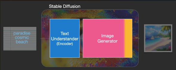
- The text understanding component is actually the text encoder used within CLIP.
- As we can see represented in the image below, Stable Diffusion takes the input text within the Text Understander component and returns a vector representing each token in the text.
- This information is then passed over to the Image Generator component which internally is composed of 2 components as well.
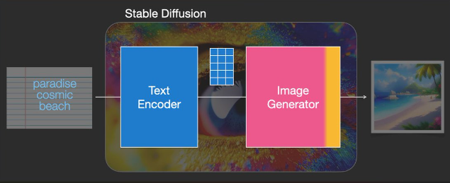
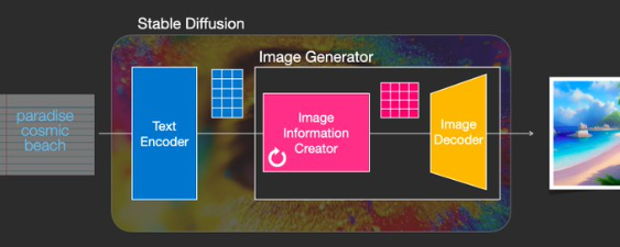
- Now, referring to the image below, let’s look at the two components within the Image Generator component.
- Image Information Creator:
- This is the ‘secret sauce’ of Stable Diffusion as it runs for a number of steps refining the information that should go in the image that will become the model’s output.
- Image Decoder:
- This component takes the processed information and paints the picture.
- Image Information Creator:
- Let’s zoom out for a second and look at the higher level components we have so far all working together for the image generation task:
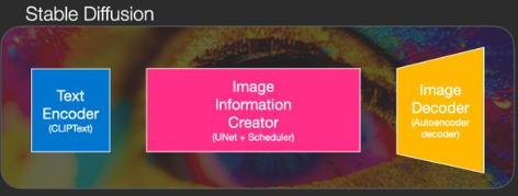
- All the 3 components above are actually individual neural networks working together, specifically, they are:
- CLIPText: Used to encode the text
- U-Net + scheduler: Used to gradually process image information(latent diffusion)
- Autoencoder Decoder: paints the final image

-
Above we can see the steps that Stable Diffusion takes to generate its images.
-
Lastly, let’s zoom into the image decoder and get a better understanding of its inner workings. Remember the image decoder is one of the two components the image generator comprises of
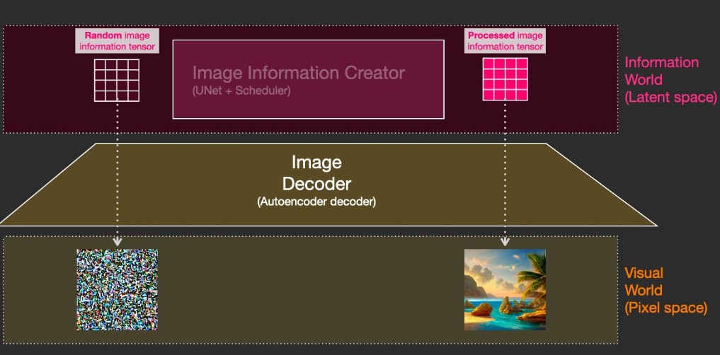
- The random vector is considered to be random noise.
- Stable Diffusion is able to obtain it’s speed from the fact that the processing happens in the latent space (which needs less calculations as compared to the pixel space).
Dream Studio
- Dream Studio is Stable Diffusion’s AI Art Web App Tool.
- DreamStudio is a new suite of generative media tools engineered to grant everyone the power of limitless imagination and the effortless ease of visual expression through a combination of natural language processing and revolutionary input controls for accelerated creativity.
Midjourney
- Midjourney is an independent research lab exploring new mediums of thought and expanding the imaginative powers of the human species.
- Midjourney has not made it’s architecture details publicly available, but one has to think they still leverage diffusion models in some fashion.
- While Dall-E 2 creates more realistic images, MidJourney shines in adapting real art styles into creating an image of any combination of things your heart desires.

DALL-E 2
- DALL-E 2 utilized diffusion models to create its images and was created by OpenAI.
- DALL-E 2 can make realistic edits to existing images from a natural language caption.
- It can add and remove elements while taking shadows, reflections, and textures into consideration.
- DALL-E 2 has learned the relationship between images and the text used to describe them.
- It uses diffusion, which starts with a pattern of random dots and gradually alters that pattern towards an image when it recognizes specific aspects of that image.
- OpenAI has limited the ability for DALL-E 2 to generate violent, hate, or adult images.
- By removing the most explicit content from the training data, OpenAI has minimized DALL-E 2’s exposure to these concepts.
- They have also used advanced techniques to prevent photorealistic generations of real individuals’ faces, including those of public figures.
- Among the most important building blocks in the DALL-E 2 architecture is CLIP to function as the main bridge between text and images.
Related: CLIP (Contrastive Language-Image Pre-Training)
- While CLIP does not use a diffusion model, it is essential to understand DALL-E 2 so let’s do a quick recap of CLIP’s architecture.
- CLIP is a neural network trained on a variety of (image, text) pairs.
- It can be instructed in natural language to predict the most relevant text snippet, given an image, without directly optimizing for the task, similarly to the zero-shot capabilities of GPT-2 and 3.
- CLIP is a multi-modal vision and language model.
- It can be used for image-text similarity and for zero-shot image classification.
- CLIP uses a ViT like transformer to get visual features and a causal language model to get the text features.
- Both the text and visual features are then projected to a latent space with identical dimension. The dot product between the projected image and text features is then used as a similar score.
- CLIP enables us to take textual phrases and understand how they map onto images
Gallery
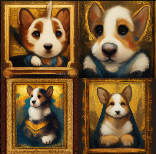
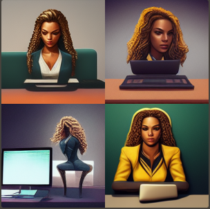
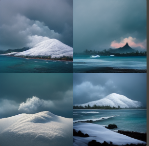
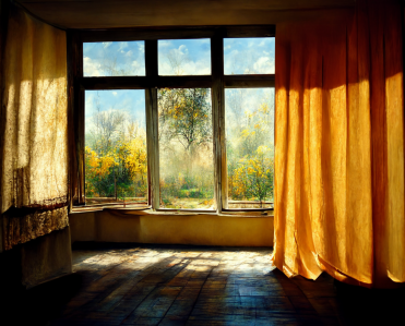
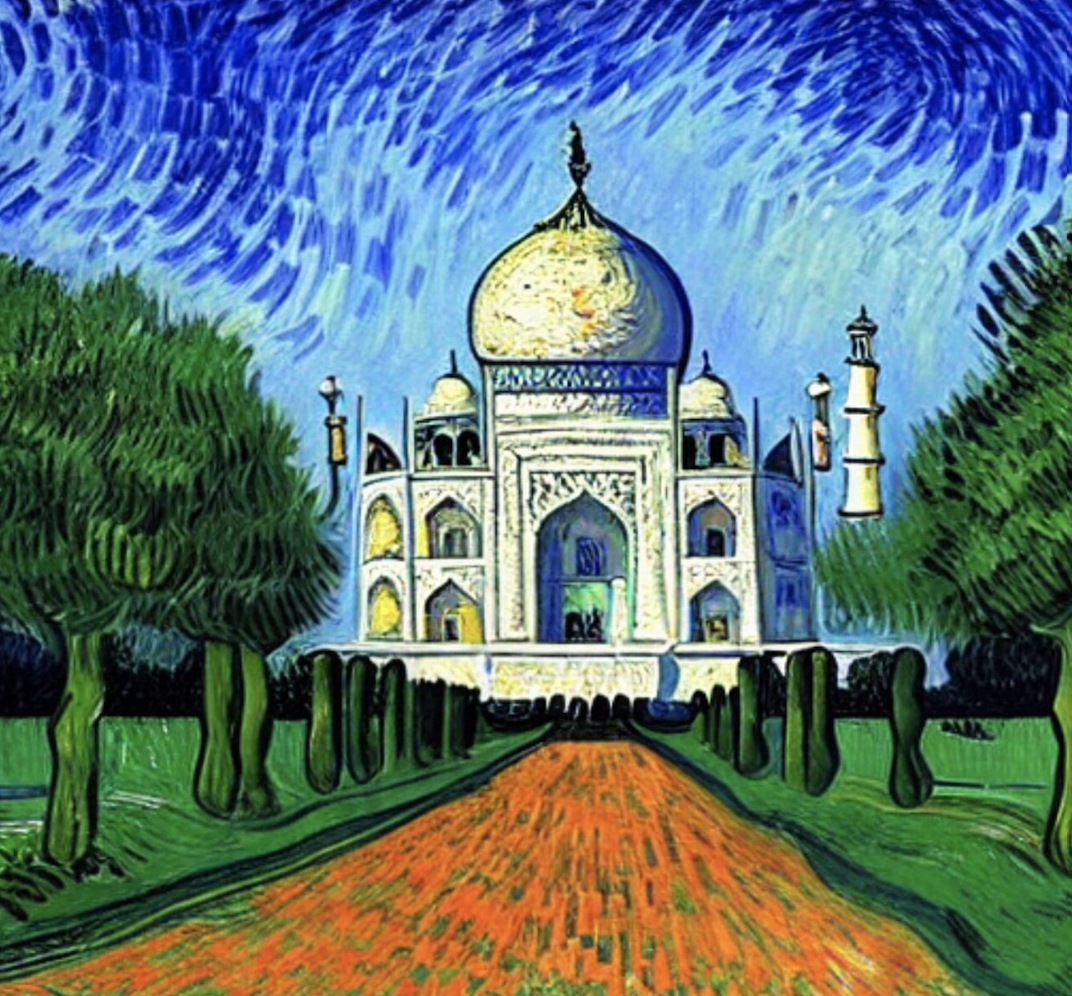
- Showcasing a few images generated via Diffusion Models along with their text prompts given:
- A Corgi puppy painted like the Mona Lisa:
- Beyonce sitting at a desk and coding:
- Snow in Hawaii:
- Sun coming in from a big window with curtains and casting a shadow on the rest of the room, artistic style:
- The Taj Mahal painted in Starry Night by Vincent Van Gogh:
Final Words
- Diffusion models are a conceptually simple and elegant approach to the problem of generating data. Their State-of-the-Art results combined with non-adversarial training has propelled them to great heights, and further improvements can be expected in the coming years given their nascent status.
- In particular, Diffusion models have been found to be essential to the performance of cutting-edge models like DALL-E 2.
References
- Diffusion models Vs GANs: Which one to choose for Image Synthesis
- Diffusion models
- Introduction to Diffusion Models for Machine Learning
- What are Diffusion Models?
- Denoising Diffusion Probabilistic Models by Ho et. al
- Lil’Log: Diffusion Models
- Assembly AI: Diffusion Models for Machine Learning Introduction
- Google ML Crashcourse on GANs
- Wikipedia: Markov Chain
- AI Summer: Latent Variable Models
- Diffusion Models Beat GANs on Image Synthesis
- Jay Alammar’s Stable Diffusion Twitter thread
- Hugging Face Stable Diffusion
- Towards Data Science: DALL-E 2 Explained
- Hugging Face’s Training with Diffusers notebook
- Hugging Face Diffusers Intro notebook
Further Reading
- Deep Unsupervised Learning using Nonequilibrium Thermodynamics 2015
- Denoising Diffusion Probabilistic Models 2020
- Improved Denoising Diffusion Probabilistic Models 2021
- Diffusion Models Beat GANs on Image Synthesis 2021
Citation
If you found our work useful, please cite it as:
@article{Chadha2020DistilledDiffusionModels,
  title   = {Diffusion Models},
  author  = {Chadha, Aman and Jain, Vinija},
  journal = {Distilled AI},
  year    = {2020},
  note    = {\url{https://aman.ai}}
}