Overview
- Here we will go over common errors in training models
Multicollinearity
- Multicollinearity refers to the high correlation between input features in a dataset, which can adversely affect the performance of machine learning models. To identify multicollinearity, one can calculate the Pearson correlation coefficient or the Spearman correlation coefficient between the input features. The Pearson correlation coefficient measures the linear relationship between variables, while the Spearman correlation coefficient assesses the monotonic relationship between variables.
- Creating a heatmap by visualizing the correlation coefficients of input features can effectively reveal multicollinearity. In the heatmap, lighter colors indicate a high correlation, while darker colors indicate a low correlation.
- To mitigate multicollinearity, one approach is to employ Principal Component Analysis (PCA) as a data preprocessing step. PCA leverages the existing correlations among input features to combine them into a new set of uncorrelated features. By applying PCA, multicollinearity can be automatically addressed. After PCA transformation, a new heatmap can be generated to confirm the reduced correlation among the transformed features.
- For a practical demonstration of removing multicollinearity using PCA, you may refer to the article “How do you apply PCA to Logistic Regression to remove Multicollinearity?” to gain hands-on experience in its application.
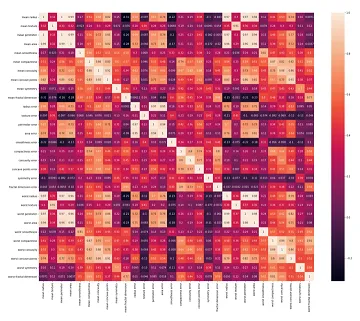
- (Source image)
Randomness
- Randomness plays a role in machine learning models, and the random state is a hyperparameter used to control the randomness within these models. By using an integer value for the random state, we can ensure consistent results across different executions. However, relying solely on a single random state can be risky because it can significantly affect the model’s performance.
- For instance, consider the train_test_split() function, which splits a dataset into training and testing sets. The random_state hyperparameter in this function determines the shuffling process prior to the split. Depending on the random state value, different train and test sets will be generated, and the model’s performance is highly influenced by these sets.
- To illustrate this, let’s look at the root mean squared error (RMSE) scores obtained from three linear regression models, where only the random state value in the train_test_split() function was changed:
- Random state = 0 → RMSE: 909.81
- Random state = 35 → RMSE: 794.15
- Random state = 42 → RMSE: 824.33
- As observed, the RMSE values vary significantly depending on the random state.
- To mitigate this issue, it is recommended to run the model multiple times with different random state values and calculate the average RMSE score. However, performing this manually can be tedious. Instead, cross-validation techniques can be employed to automate this process and obtain a more reliable estimate of the model’s performance.
- Relying on a single random state in machine learning models can yield inconsistent results, and it is advisable to leverage cross-validation methods to mitigate this issue.
Data leaks
- Data leakage occurs when preprocessing and transforming data, leading to biased and unreliable results. Two common scenarios where data leakage can occur are during feature standardization and when applying transformations to the data.
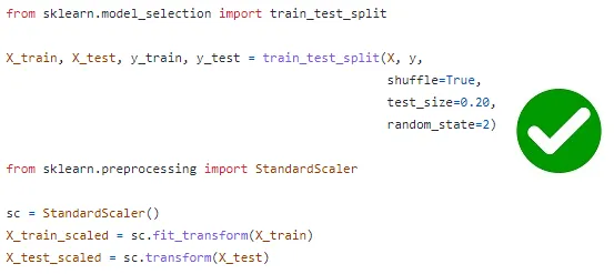
-
(Source image)
- In the case of feature standardization, data leakage happens when the entire dataset is standardized before splitting into training and test sets. This is problematic because the test set, which is derived from the full dataset, is used to calculate the mean and standard deviation for standardization. To prevent data leakage, it is recommended to perform feature standardization separately on the training and test sets after the data split.
- Similarly, data leakage can occur when applying transformations to the data, such as using functions like StandardScaler or PCA. If the fit() method of these functions is called twice, once on the training set and again on the test set, new values are computed based on the test set, leading to biased results. To avoid data leakage, it is essential to call the fit() method only on the training set.
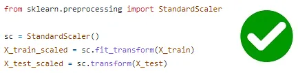
-
(Source image)
- By addressing these issues and avoiding data leakage, we can ensure the integrity and reliability of machine learning models.
- Data leakage can compromise the accuracy and generalizability of machine learning models. It is crucial to be cautious during preprocessing and transformation steps to prevent unintentional data leakage. By adhering to best practices and following proper procedures, we can minimize the risk of data leakage and obtain more robust and trustworthy results.
Underfitting
- Underfitting occurs when a model is too simple and fails to learn essential patterns in the training data. It results in poor performance on both the training data and new, unseen data. Underfitting can be identified by analyzing the learning curve, where the model’s performance remains consistently low.
- To avoid underfitting, the following techniques can be employed:
- Increase the complexity of the model.
- Increase the number of input features.
- Allow the model to train for a longer duration.
Overfitting
- Overfitting happens when a model is overly complex and tries to memorize the training data instead of learning underlying patterns. It performs well on the training data but fails to generalize to new, unseen data. Overfitting can be detected through the learning curve, which shows a significant gap between the performance on the training set and the performance on the validation or test set.
- To avoid overfitting, the following techniques can be employed:
- Increase the number of training examples.
- Use techniques such as feature selection, creating ensembles, dimensionality reduction, regularization, cross-validation, and early stopping.
- Utilize neural network-specific techniques like dropout, L1 and L2 regularization, early stopping, data augmentation, and noise regularization.
- When utilizing the categorical_crossentropy loss function, it is essential to apply one-hot encoding to scalar value labels. Failure to do so will result in an error. The error arises because the categorical_crossentropy function expects one-hot encoded labels as input.
- To avoid this error, you can take the following measures:
- Use the sparse_categorical_crossentropy loss function instead of categorical_crossentropy. This function does not require one-hot encoding.
- Perform one-hot encoding on the labels and continue using the categorical_crossentropy loss function. One-hot encoding transforms scalar labels into n-element vectors, where n represents the number of classes. The to_categorical() function can be employed for this purpose.
- By adhering to these guidelines and ensuring proper one-hot encoding, you can effectively prevent errors and employ the categorical_crossentropy loss function accurately in your deep learning models.
Small dataset for complex algorithms
- Deep learning algorithms, such as neural networks, are primarily designed to excel when working with large datasets comprising millions or thousands of millions of training instances. In the case of small datasets, their performance is considerably limited.
- In fact, there are instances where deep learning algorithms perform even worse than conventional machine learning algorithms when applied to small datasets.
Failure to detect outliers in data
- Outliers are often present in real-world datasets, representing data points that deviate significantly from the majority of other data points. These outliers can be visually identified when plotting the data, as they appear distinctly separate from the rest.
- Methods for outlier detection:
- Several techniques can be employed to detect outliers, including:
- IQR-based detection
- Elliptic envelope
- Isolation forest
- One-class SVM
- Local outlier factor (LOF)
- Handling outliers:
- When dealing with outliers, it is crucial to carefully consider their significance. Simply removing outliers without understanding their underlying story is not recommended. If an outlier carries valuable information relevant to the problem at hand, it should be retained and accounted for in subsequent analysis. However, outliers resulting from data collection errors can be safely removed. Neglecting to address unnecessary outliers can introduce bias to the model and potentially lead to the omission of important patterns within the data.
Failure to verify model assumptions
- When constructing models, we often work under specific assumptions. These assumptions serve as the foundation for accurate predictions, provided they are not violated. Therefore, it is crucial to validate the underlying assumptions once the model is built.
- Examples of validating model assumptions:
- Normality assumption in linear regression: One assumption is that the residuals (the differences between observed and predicted values) in a linear regression model follow a normal distribution with a mean of zero and a fixed standard deviation. To verify this, we can create a histogram of the residuals and ensure they approximate a normal distribution. Additionally, calculating the mean of the residuals and confirming its proximity to zero reinforces this assumption.
- Histogram depicting the distribution of residuals (Image by author)
- Independence assumption in linear regression: Another assumption is that the residuals in a linear regression model are uncorrelated or independent. We can verify this assumption by generating a residual plot, examining the pattern of the residuals to ensure no systematic correlation exists between them.
Failure to utilize a validation set for hyperparameter tuning
- In the process of hyperparameter tuning, it is essential to employ a distinct dataset known as the validation set, in addition to the training and testing datasets. Utilizing the same training data for hyperparameter tuning can result in data leakage, undermining the model’s ability to generalize to new, unseen data.
- To ensure an effective approach, the training set is utilized for fitting the model parameters, the validation set is dedicated to fine-tuning the model’s hyperparameters, and the test set is employed to evaluate the model’s performance. By adhering to this methodology, we can enhance the model’s overall effectiveness and robustness.
- Using a validation set for hyperparameter tuning is crucial for several reasons:
- Preventing Overfitting: Hyperparameter tuning involves adjusting the settings of the model to optimize its performance. Without a validation set, tuning is performed on the same data used for training, which can lead to overfitting. Overfitting occurs when the model becomes too specific to the training data and performs poorly on new, unseen data. By utilizing a separate validation set, we can assess the model’s performance on unseen data and make more informed decisions during hyperparameter tuning.
- Evaluating Generalization: The primary goal of machine learning is to build models that can generalize well to unseen data. A validation set allows us to evaluate the model’s performance on data it hasn’t encountered during training. By tuning the hyperparameters based on the validation set’s performance, we increase the chances of the model’s ability to generalize and perform well on new data.
- Avoiding Data Leakage: Data leakage refers to situations where information from the test or validation set unintentionally leaks into the training process, leading to overly optimistic performance estimates. If the same data is used for both training and hyperparameter tuning, the model can indirectly “learn” about the validation data and bias the tuning process. By using a separate validation set, we ensure that the tuning process remains independent and unbiased.
Less data for training
- Allocating an adequate amount of data for the training set is crucial for effective model learning and generalization. The following points highlight the importance of allocating a sufficient portion of the dataset for training:
- Enhanced Learning: A larger training set allows the model to access a wider range of examples, enabling it to capture diverse patterns and relationships present in the data. With more data, the model can learn more robust representations and make better predictions. Therefore, it is advisable to allocate a significant portion of the data for training.
- Generalization Improvement: A well-trained model should be capable of performing well on unseen data. By providing a substantial training set, the model has a better chance of learning the underlying patterns that generalize to new instances. This helps in improving the model’s ability to make accurate predictions on real-world data.
- Additionally, here are some guidelines for choosing the training set size:
- For small datasets containing hundreds or thousands of samples, it is recommended to allocate approximately 70%-80% of the data for training. This ensures that the model has access to a sufficient number of examples to learn meaningful patterns and relationships.
- For large datasets with millions or billions of samples, a higher allocation, such as 96%-98% of the data, can be used for training. The abundance of data allows the model to effectively capture complex patterns and make accurate predictions.
- Remember that the specific allocation percentages may vary based on the nature of the dataset and the specific problem at hand. It is important to strike a balance between the training set size and the availability of data for validation and testing purposes.
- By allocating a substantial amount of data for the training set, we provide the model with ample opportunities to learn and generalize effectively, leading to improved performance on unseen data.
Accuracy metric used to evaluate models with data imbalance
- When dealing with class imbalance, where one class has a significantly larger number of instances than the other, using accuracy as an evaluation metric can be misleading. It is important to consider the following points:
- Imbalanced Class Distribution: In datasets with class imbalance, the majority class dominates the overall distribution, while the minority class is underrepresented. For instance, in a spam email detection dataset, there may be 9900 instances of the “Not spam” class and only 100 instances of the “Spam” class.
- Accuracy Bias: Accuracy alone is not a reliable metric in the presence of class imbalance. A model trained on such data may achieve a high accuracy score by simply predicting the majority class (i.e., “Not spam”). However, this accuracy does not reflect the model’s performance in capturing the minority class (i.e., “Spam”).
- Failure to Capture Minority Class: Due to the imbalanced nature of the dataset, the model may struggle to learn the patterns and characteristics of the minority class. Consequently, it may perform poorly in predicting instances belonging to the minority class, leading to false negatives or misclassifications.
- To properly evaluate models with class imbalance, it is recommended to use evaluation metrics that provide a more comprehensive understanding of the model’s performance. Some commonly used metrics in this context include:
- Precision and Recall: Precision measures the proportion of correctly predicted positive instances (e.g., “Spam”) out of all instances predicted as positive. Recall, on the other hand, calculates the proportion of correctly predicted positive instances out of all actual positive instances. These metrics are more informative about the model’s performance on the minority class.
- F1-Score: The F1-score is the harmonic mean of precision and recall. It provides a balanced evaluation of the model’s performance by considering both precision and recall. This metric is useful for assessing models in imbalanced datasets.
- Area Under the Receiver Operating Characteristic Curve (AUC-ROC): The AUC-ROC score quantifies the model’s ability to discriminate between the classes across different classification thresholds. It provides a holistic view of the model’s performance, taking into account both true positive and false positive rates.
- By using these metrics, we can obtain a more accurate assessment of the model’s performance, specifically in capturing the minority class and mitigating the bias introduced by class imbalance.
Omitting data normalization
- Neglecting to normalize the input and output data can have adverse effects on the performance of neural networks.
- It is crucial to ensure that the data is distributed with a mean close to zero and a standard deviation of approximately one before feeding it into the network.
Using excessively large batch sizes
- Employing a very large batch size can hinder the model’s ability to generalize well and may negatively impact the accuracy during training.
- This is due to reduced stochasticity in the gradient descent process, which can prevent the network from effectively navigating the optimization landscape.
Neglecting to apply regularization techniques
- Regularization serves a dual purpose of preventing overfitting and aiding in handling noise and outliers in the data.
- For efficient and stable training, it is important to incorporate appropriate regularization techniques into the model.
Selecting an incorrect learning rate
- The choice of learning rate plays a critical role in training the network. An improper learning rate can make the training process challenging or even infeasible.
- It is essential to find an appropriate learning rate that facilitates effective convergence and avoids issues such as slow training or unstable optimization.
Using an incorrect activation function for the output layer
- Employing an inappropriate activation function for the output layer can result in the network failing to produce the desired range of values.
- For instance, using ReLU activation on the output layer may restrict the network to only positive output values. It is important to select an activation function that aligns with the desired output behavior.
Employing an excessively deep network or an incorrect number of hidden units
- Deeper networks are not always better, and using an incorrect number of hidden units can impede training progress. In some cases, a very small number of units may lack the capacity to express the desired objective, while an excessively large number of units can lead to slow and computationally intensive training, making it challenging to remove residual noise during the training process.
- Finding the right balance in terms of the depth of the network and the number of hidden units involves a combination of experimentation, analysis, and validation. Here are some approaches that can help in finding the optimal balance:
- Start with simpler architectures: It is often recommended to start with a simpler architecture and gradually increase its complexity. Begin with a shallow network and a moderate number of hidden units. Train and evaluate the model’s performance to establish a baseline.
- Evaluate performance on validation data: Use a separate validation dataset to assess the model’s performance as you modify its architecture. Monitor key performance metrics such as accuracy, loss, or other relevant metrics specific to your problem domain. This can provide insights into how the changes in architecture affect the model’s ability to generalize.
- Explore different architectures: Experiment with different network architectures, varying the depth and number of hidden units. Consider increasing the depth of the network gradually, adding more hidden units to specific layers, or even exploring different layer configurations (e.g., convolutional layers, recurrent layers). Evaluate each architecture on the validation set to compare their performance.
- Regularization techniques: Apply regularization techniques such as dropout, L1/L2 regularization, or batch normalization to control overfitting and improve generalization. Regularization can help prevent the network from becoming overly complex and reduce the risk of overfitting, especially when dealing with larger architectures.
- Cross-validation: Perform cross-validation, particularly when the dataset size is limited. This involves splitting the data into multiple folds, training the model on different combinations of training and validation sets, and evaluating its performance. Cross-validation helps in obtaining a more robust estimate of the model’s performance and can guide the selection of the optimal architecture.
- Consider computational constraints: Take into account the available computational resources and time constraints. Deep networks with a large number of parameters can be computationally expensive to train, especially with limited resources. Ensure that the chosen architecture strikes a balance between performance and computational feasibility.
- Domain expertise and intuition: Leverage your domain knowledge and intuition to guide the architectural choices. Consider the specific characteristics of your problem and the nature of the data. For example, in image processing tasks, convolutional neural networks (CNNs) are commonly used due to their ability to capture spatial features.
- Remember that finding the right balance is an iterative process. It may require several rounds of experimentation, evaluation, and fine-tuning. It is important to assess the trade-offs between model complexity, computational requirements, and the desired performance on both training and validation/test data.
Not Accounting For Data Drift And Semantic Shift
- Data drift refers to the phenomenon where the statistical properties of the data change over time, leading to a discrepancy between the training data and the real-time data the model encounters during deployment. Ignoring data drift can significantly degrade the performance and accuracy of AI models.
- To address data shift and semantic shift, organizations should consider the following practices:
- Continuous data monitoring: Implement a robust data monitoring system to track and analyze changes in the input data distribution. This involves regularly collecting and analyzing new data points to identify any significant shifts or deviations from the training data. Data monitoring can be done through statistical analysis, visualization techniques, or by using specialized tools and platforms.
- Data preprocessing and feature engineering: As new data streams in, it is crucial to preprocess and engineer features to ensure compatibility with the existing model. This may involve adapting existing preprocessing steps or introducing new techniques to handle changes in data formats, data types, or feature distributions.
- Retraining and updating models: When significant data drift is detected, it may be necessary to retrain or update the AI models to capture the evolving patterns in the data. This can be done by incorporating new labeled data into the training set or by using techniques such as transfer learning, where a pre-trained model is fine-tuned with the new data. Regular model reevaluation and refinement are essential to ensure models remain accurate and effective over time.
- Ensemble modeling: Ensemble modeling involves combining predictions from multiple models to enhance performance and robustness. By training and maintaining multiple models with different architectures or trained on different datasets, organizations can leverage diversity in model predictions to mitigate the impact of data drift.
- Feedback loops and user feedback: Establish feedback mechanisms that allow users or domain experts to provide insights, flag issues, and highlight areas where the model’s predictions may be deviating from the expected behavior. User feedback can provide valuable information for understanding data shift and addressing potential problems in model performance.
- Human-in-the-loop approach: Incorporate human expertise and intervention into the model’s decision-making process. Human reviewers or validators can play a role in ensuring the model’s predictions align with domain knowledge and handle cases where the model’s performance may be affected by data drift.
- Regular model audits and performance evaluations: Conduct periodic audits and evaluations of the model’s performance to identify any degradation or deviation from the desired accuracy. This can involve comparing model predictions with ground truth data, conducting A/B testing, or employing external evaluation techniques.
- Data governance and documentation: Implement robust data governance practices to track and document changes in data sources, transformations, and preprocessing steps. Maintaining a comprehensive record of data shifts and the corresponding model updates can aid in understanding the impact of data drift and ensuring transparency and accountability.