Primers • Bias-Variance Tradeoff
- Overview
- Bias
- Variance
- Mathematical Interpretation
- Bias and Variance: A Visual Perspective
- Underfitting and Overfitting
- The Bias-Variance Tradeoff
- Total Error
- Balancing Overfitting and Underfitting
- Summary
- References
- Citation
Overview
- Understanding bias and variance is critical in machine learning as they define a fundamental tradeoff in model design. Striking the right balance between these two factors is essential to improve model accuracy and avoid common pitfalls like overfitting and underfitting. This balance is vital for ensuring a model performs well across both training and testing datasets, forming the foundation for robust predictive performance in diverse applications.
- Bias refers to the error introduced by approximating a complex problem with a simpler model. High bias can cause underfitting, where the model fails to capture the underlying patterns in the data. Variance, on the other hand, measures the model’s sensitivity to small fluctuations in the training data. High variance can lead to overfitting, where the model captures noise instead of the signal.
- Understanding the mathematical interpretations and practical implications of bias and variance helps in designing models that generalize well. A well-balanced model minimizes both bias and variance, enabling accurate predictions and robust performance across different datasets.
Bias
- In data science, bias refers to the error arising from incorrect assumptions in the learning algorithm. It measures how much the predicted values deviate from the actual values on average. A high-bias model tends to oversimplify the data, leading to inaccuracies on both the training and testing datasets.
Key Takeaways
- Definition: Bias is the difference between the average model prediction and the true value being predicted.
- Characteristics of High Bias Models:
- Pay minimal attention to training data.
- Oversimplify the model structure.
- Lead to high errors in both training and testing datasets.
Example
- Linear models used for predicting highly nonlinear data are examples of high-bias models, as they fail to capture the underlying complexity of the dataset.
Variance
- Variance measures the model’s sensitivity to fluctuations in the training dataset. High-variance models are highly tuned to training data but fail to generalize to unseen data, resulting in poor performance on testing datasets.
Key Takeaways
- Definition: Variance reflects the spread of model predictions for a given data point.
- Characteristics of High Variance Models:
- Learn excessively from the training data.
- Perform well on training data but poorly on test data due to overfitting.
Example
- Complex models like decision trees that are deeply trained on noisy datasets exhibit high variance as they memorize training data patterns.
Mathematical Interpretation
-
Let \(Y\) be the variable we aim to predict and \(X\) be the input features. The relationship between them is expressed as:
\[Y = f(X) + e\]- where:
- \(f(X)\) represents the true function.
- \(e\) is the error term, typically assumed to be normally distributed with a mean of 0.
- where:
-
A model, \(\hat{f}(X)\), approximates \(f(X)\) using a learning algorithm. The expected squared error at a point \(x\) can be decomposed as:
-
Breaking this down further:
\[\text{Err}(x) = (\mathbb{E}[\hat{f}(x)] - f(x))^2 + \mathbb{E}[(\hat{f}(x) - \mathbb{E}[\hat{f}(x)])^2] + \sigma_e^2\]- where:
- \((\mathbb{E}[\hat{f}(x)] - f(x))^2\) is the bias squared.
- \(\mathbb{E}[(\hat{f}(x) - \mathbb{E}[\hat{f}(x)])^2]\) is the variance.
- \(\sigma_e^2\) is the irreducible error.
- where:
Irreducible Error
- Irreducible error represents noise inherent in the data that cannot be eliminated, regardless of model complexity.
Bias and Variance: A Visual Perspective
Bulls-Eye Diagram
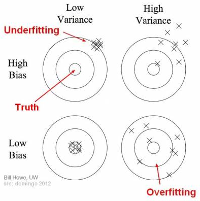
- The bulls-eye diagram below (source) visualizes bias and variance:

- The center represents the perfect prediction.
- High bias: Predictions are consistently far from the center.
- High variance: Predictions are scattered widely around the center.
Underfitting and Overfitting
- Underfitting:
- Occurs when the model is too simple to capture data patterns.
- Associated with high bias and low variance.
- Examples: Using a linear model for nonlinear data.
- Overfitting:
- Occurs when the model captures both data patterns and noise.
- Associated with low bias and high variance.
- Examples: Deep decision trees trained on noisy data.
- Below is a representation of the above concepts (source):

The Bias-Variance Tradeoff
- The bias-variance tradeoff describes the balance required to build a model that generalizes well across datasets.
Key Insights
- Low Bias, Low Variance: Optimal goal, but challenging to achieve.
- High Bias, Low Variance: Simple models, prone to underfitting.
- Low Bias, High Variance: Complex models, prone to overfitting.
Example
- Studying for an exam using only sample papers might help with familiar questions (low bias) but could fail for unfamiliar ones (high variance). Broadening the study material results in better generalization.
Total Error
- The total error can be expressed as:
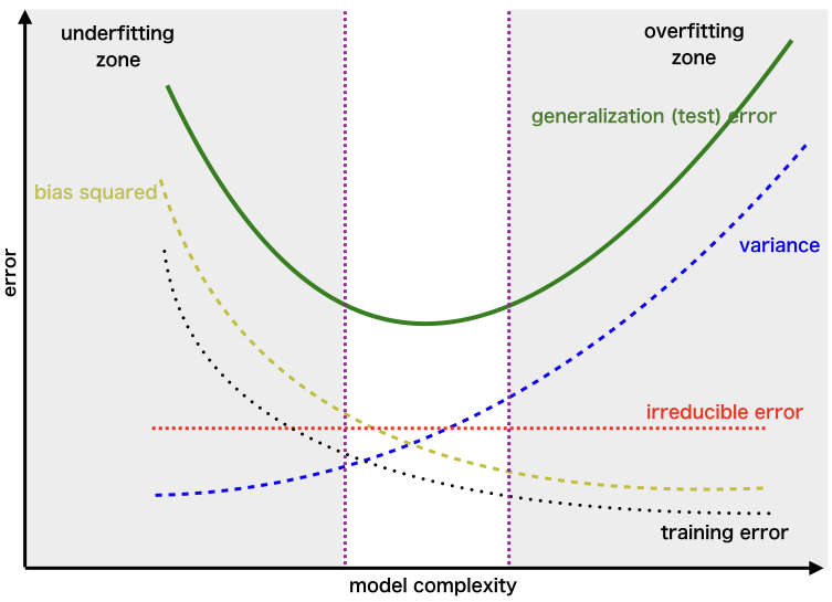
- Below is a plot (source) illustrating the relationship between these components:

- Striking the right balance between bias and variance minimizes the total error, avoiding both overfitting and underfitting.
The Goal: Low Bias and Low Variance
-
Low bias and low variance are both desired because they indicate that the model is generalizing well to unseen data. Here’s why:
- Low Bias:
- Bias reflects the error due to overly simplistic assumptions in the model.
- A model with high bias might underfit the data, meaning it fails to capture the underlying patterns or relationships, leading to poor performance on both training and test datasets.
- Low bias ensures the model is flexible enough to learn the true patterns in the data.
- Low Variance:
- Variance reflects the error due to sensitivity to small fluctuations in the training data.
- A model with high variance might overfit the data, meaning it captures noise or specific details that do not generalize to new data.
- Low variance ensures the model’s performance is consistent across different datasets.
- Low Bias:
- The ultimate goal is to find a balance between bias and variance — a sweet spot often referred to as the bias-variance tradeoff. Achieving low bias and low variance simultaneously minimizes the total error (sum of bias error, variance error, and irreducible error), resulting in a robust model.
- However, it is worth noting that in practice, there is often a tradeoff between bias and variance, and perfect minimization of both is rarely achievable.
Balancing Overfitting and Underfitting
- Overfitting occurs when a model learns the sampling error/noise from the training data, and thus fails to generalize to unseen data.
- Underfitting occurs when a model is too simple to capture the underlying patterns in the data.
- Based on the stage of model development, here are a variety of techniques to prevent overfitting and underfitting. By employing these techniques and regularly monitoring performance, you can design robust models that generalize well to unseen data while avoiding overfitting and underfitting. Here’s the updated writeup with label smoothing added under “Regularization Through Data”:
Techniques to Prevent Overfitting
- Data-Related Techniques:
- Increase Training Data:
- Collect more data to ensure the model has diverse examples.
- Use data augmentation (e.g., flipping, rotating, scaling images for computer vision, or backtranslation for NLP) to artificially increase the size of the dataset.
- Data Cleaning:
- Remove noise and irrelevant data points that might cause the model to memorize instead of generalize.
- Cross Validation:
- Use techniques like k-fold cross validation, particularly effective in low-data regimes, to test the model on different subsets of the data, ensuring it generalizes well across various samples.
- Increase Training Data:
- Model Architecture:
- Decrease Model Complexity/Simplify the Model:
- Reduce the number of layers or nodes in deep learning models to avoid fitting noise.
- Regularization (L1/L2/Elastic Net/Dropout):
- Add constraints to the model’s complexity:
- L1 Regularization: Encourages sparsity by adding a penalty proportional to the absolute values of weights.
- L2 Regularization: Penalizes large weights by adding a penalty proportional to their squared values.
- ElasticNet: Combines L1 and L2 regularization.
- Dropout: Randomly disable neurons during training to prevent the model from becoming overly reliant on specific pathways.
- A detailed discourse on regularization is available in our Regularization primer.
- Decrease Model Complexity/Simplify the Model:
- Training Adjustments:
- Early Stopping:
- Monitor the model’s performance on a validation set during training. Stop training when validation loss starts increasing (i.e., stops improving/decreasing), even if training loss decreases.
- Batch Normalization:
- Normalize inputs within a network layer to stabilize learning and reduce sensitivity to initialization.
- Early Stopping:
- Ensemble Techniques:
- Bagging (e.g., Random Forest):
- Train multiple models on random subsets of the data.
- Boosting (e.g., Gradient Boosting, XGBoost):
- Sequentially train models where each new model corrects the errors of the previous one.
- Stacking:
- Combine predictions from multiple models using another model as a meta-learner.
- Bagging (e.g., Random Forest):
- Regularization Through Data:
- Label Smoothing:
- Reduce overconfidence in predictions by softening the target labels (e.g., assigning 0.9 instead of 1 to the true class). This regularization technique encourages the model to output probability distributions that are less certain, which helps reduce overfitting and improves generalization.
- Adversarial Training:
- Train the model with slightly modified input data to make it robust to small perturbations.
- Label Smoothing:
Techniques to Prevent Underfitting
- Data-Related Techniques:
- Increase Data Quality:
- Ensure the dataset is diverse, comprehensive, and representative of the problem space.
- Feature Engineering:
- Extract or create meaningful features from the raw data to make patterns more discernible.
- Ensure important features are not excluded during preprocessing or feature selection.
- Perform transformations such as polynomial features or domain-specific enhancements.
- Increase Data Quality:
- Model Architecture:
- Increase Model Complexity:
- Add more layers, neurons, or parameters to increase the expressive capacity of the model to learn complex patterns.
- Use Appropriate Model Types:
- Use advanced models like neural networks, decision trees, or ensemble methods for problems with complex patterns.
- Increase Model Complexity:
- Training Adjustments:
- Train for Longer:
- Allow the model to run for more epochs to learn patterns that may require more time.
- Hyperparameter Tuning:
- Use techniques like grid search, random search, or Bayesian optimization to fine-tune hyperparameters such as learning rates, batch sizes, and other training parameters to achieve better performance.
- Train for Longer:
- Regularization:
- Avoid Excessive Regularization:
- Re-tune the regularization strength \(\lambda\). Keep regularization terms at appropriate levels to avoid restricting the model’s capacity too much.
- Avoid Excessive Regularization:
Key Metrics for Monitoring Overfitting and Underfitting
- Training vs. Validation Error:
- A large gap (low training error, high validation error) indicates overfitting.
- High error in both training and validation indicates underfitting.
- Bias-Variance Trade-Off:
- Assess whether the model’s errors are due to bias (underfitting) or variance (overfitting).
- Learning Curves:
- Plot error against training size or epochs to diagnose training issues.
Overfitting and underfitting: Common challenges in low-data scenarios
- Both overfitting and underfitting are common challenges in low-data scenarios, due to the trade-off between model complexity and data limitations.
- The key is to adopt techniques that maximize the effective use of data while ensuring the model’s complexity aligns with the data’s capacity to support it.
Overfitting in Low-Data Scenarios
-
Overfitting occurs when the model learns patterns that are specific to the training data, including noise or irrelevant details, which do not generalize to new data.
- Why it’s common:
- Limited data diversity: With insufficient data, the training set may not represent the true variability of the underlying distribution, leading the model to memorize the training data instead of learning generalizable patterns.
- Complex models: Using models that are too complex (e.g., deep neural networks with many parameters) in relation to the amount of available data can cause them to fit the noise or specific idiosyncrasies of the training data.
- Lack of regularization: Inadequate use of regularization techniques (e.g., dropout, L1/L2 regularization) exacerbates overfitting, especially when the training data is sparse.
- Symptoms:
- High accuracy on the training set but poor performance on validation/test data.
Underfitting in Low-Data Scenarios
-
Underfitting occurs when the model fails to capture the underlying patterns in the data, resulting in poor performance even on the training set.
- Why it’s common:
- Overly simple models: Using models that are too simple relative to the complexity of the data (e.g., linear models for nonlinear relationships) can lead to underfitting.
- Insufficient training: In a low-data regime, there might not be enough training examples to allow the model to adequately learn patterns.
- Noise and poor feature representation: If the available data is noisy or lacks informative features, the model may struggle to find meaningful patterns.
- Strong regularization: Overuse of regularization techniques can overly constrain the model, causing it to underfit.
- Symptoms:
- Poor performance on both training and validation/test data.
Balancing Overfitting and Underfitting
-
In low-data scenarios, achieving the right balance is particularly challenging but critical. Here are some approaches:
-
Data Augmentation: Use synthetic data to increase the diversity of the training set.
-
Regularization: Apply regularization techniques judiciously to prevent overfitting while not overly constraining the model.
-
Simpler Models: Start with simpler models (fewer parameters) and incrementally increase complexity if underfitting occurs.
-
Cross-Validation: Use techniques like \(k\)-fold cross-validation to maximize data usage and improve performance estimates.
-
Careful Feature Engineering: Extract meaningful features from the data to maximize information content.
-
Summary
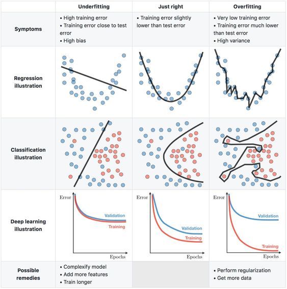
- The following table (source) summarizes the concept of Bias-Variance Tradeoff:

References
Citation
If you found our work useful, please cite it as:
@article{Chadha2020DistilledBiasVarianceTradeoff,
title   = {Bias-Variance Tradeoff},
author  = {Chadha, Aman},
journal = {Distilled AI},
year    = {2020},
note    = {\url{https://aman.ai}}
}