Primers • Bayes' Theorem
- Overview
- Bayes’ Theorem
- History
- A logical process for modern data science
- Bayesian inference
- Practical example with Python code
- Chaining Bayes’ rule
- Summary
- Further reading
- Citation
Overview
- This topic seeks to demonstrate a simple yet practical example of the application of the Bayes’ rule with Python code.
Bayes’ Theorem
- Bayes’ theorem (alternatively Bayes’ law or Bayes’ rule) has been called the most powerful rule of probability and statistics. It describes the probability of an event, based on prior knowledge of conditions that might be related to the event.
-
For example, if a disease is related to age, then, using Bayes’ theorem, a person’s age can be used to more accurately assess the probability that they have the disease, compared to the assessment of the probability of disease made without knowledge of the person’s age.
-
It is a powerful law of probability that brings in the concept of ‘subjectivity’ or ‘the degree of belief’ into the cold, hard statistical modeling. Bayes’ rule is the only mechanism that can be used to gradually update the probability of an event as the evidence or data is gathered sequentially.
-
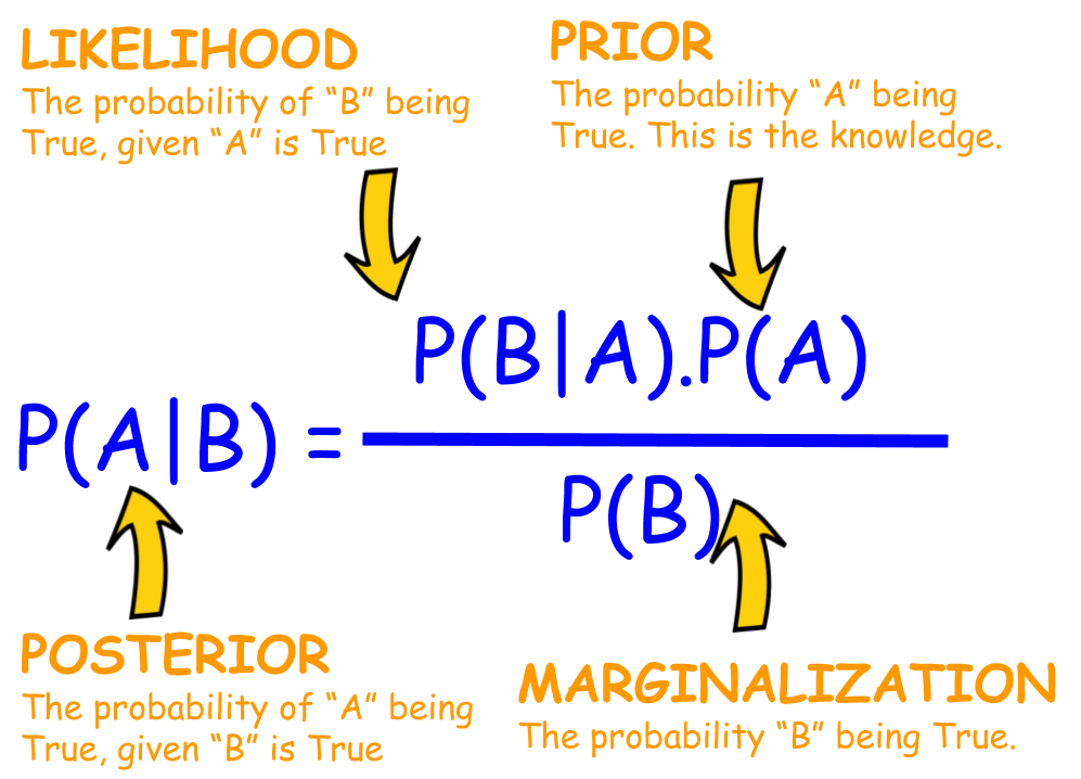
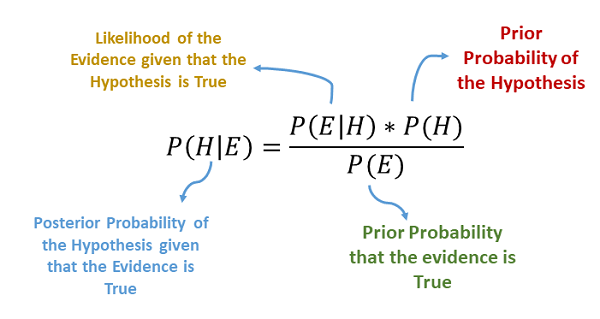
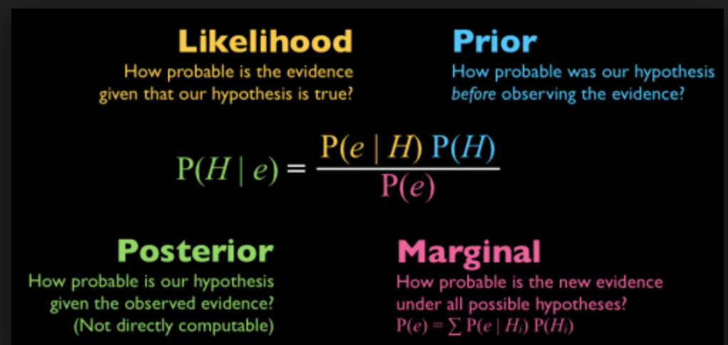
In terms of predicting the probability of occurrence of a hypothesis \(H\) given some evidence \(E\) (denoted as \(P(H \mid E)\)), Bayes’ theorem can be expressed in terms of \(P(E \mid H)\), \(P(H)\) and \(P(E)\) as:
History
-
Bayes’ theorem is named after Reverend Thomas Bayes, who first used conditional probability to provide an algorithm (his Proposition 9) that uses evidence to calculate limits on an unknown parameter, published as An Essay towards solving a Problem in the Doctrine of Chances (1763). In what he called a scholium, Bayes extended his algorithm to any unknown prior cause.
-
Independently of Bayes, Pierre-Simon Laplace in 1774, and later in his 1812 “Théorie analytique des probabilités” used conditional probability to formulate the relation of an updated posterior probability from a prior probability, given evidence.
It is a powerful law of probability that brings in the concept of ‘subjectivity’ or ‘the degree of belief’ into the cold, hard statistical modeling.
A logical process for modern data science
-
It is a logical way of doing data science.
-
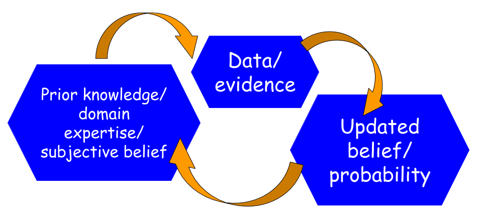
We start with a hypothesis and a degree of belief in that hypothesis. That means, based on domain expertise or prior knowledge, we assign a non-zero probability to that hypothesis.
-
Then, we gather data and update our initial beliefs. If the data support the hypothesis then the probability goes up, if it does not match, then probability goes down.
-
Sound’s simple and logical, doesn’t it? But traditionally, in the majority of statistical learning, the notion of prior is not used or not looked favorably. Also, the computational intricacies of Bayesian learning have prevented it from being mainstream for more than two hundred years.
-
But things are changing now with the advent of Bayesian inference…
If the data support the hypothesis then the probability goes up, if it does not match, then probability goes down.
Bayesian inference
-
Bayesian statistics and modeling have had a recent resurgence with the global rise of AI and data-driven machine learning systems in all aspects of business, science, and technology.
-
Bayesian inference is being applied to genetics, linguistics, image processing, brain imaging, cosmology, machine learning, epidemiology, psychology, forensic science, human object recognition, evolution, visual perception, ecology, and countless other fields where knowledge discovery and predictive analytics are playing a significant role.
Bayesian statistics and modeling have had a recent resurgence with the global rise of AI and data-driven machine learning systems
Practical example with Python code
Drug screening
-
As an example, let’s apply Bayes’ rule to a problem of drug screening (e.g. mandatory testing for federal or many other jobs which promise a drug-free work environment).
-
Suppose that a test for using a particular drug is 97% sensitive and 95% specific. That is, the test will produce 97% true positive results for drug users and 95% true negative results for non-drug users. These are the pieces of data that any screening test will have from their history of tests. Bayes’ rule allows us to use this kind of data-driven knowledge to calculate the final probability.
-
Suppose, we also know that 0.5% of the general population are users of the drug. What is the probability that a randomly selected individual with a positive test is a drug user?
-
Note, this is the crucial piece of ‘Prior’ which is a piece of generalized knowledge about the common prevalence rate. This is our prior belief about the probability of a random test subject being a drug user. That means if we choose a random person from the general population, without any testing, we can only say that there is a 0.5% chance of that person being a drug-user.
-
How to use Bayes’ rule then, in this situation?
-
We will write a custom function that accepts the test capabilities and the prior knowledge of drug user percentage as input and produces the output probability of a test-taker being a user based on a positive result.
-
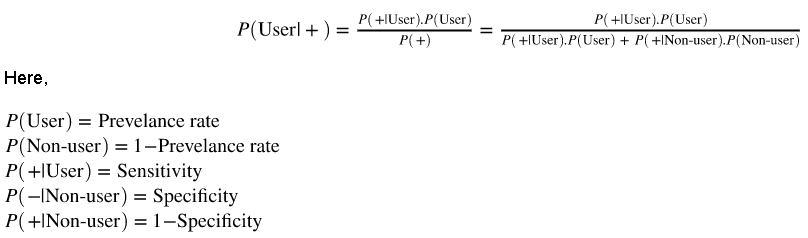
Here is the formula for computing as per the Bayes’ rule:
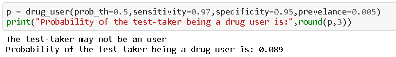
- If we run the function with the given data, we get the following result,
What is fascinating here?
-
Even with a test that is 97% correct for catching positive cases, and 95% correct for rejecting negative cases, the true probability of being a drug-user with a positive result is only 8.9%!
-
If you look at the computations, this is because of the extremely low prevalence rate. The number of false positives outweighs the number of true positives.
-
For example, if 1000 individuals are tested, there are expected to be 995 non-users and 5 users. From the 995 non-users, 0.05 × 995 ≃ 50 false positives are expected. From the 5 users, 0.95 × 5 ≈ 5 true positives are expected. Out of 55 positive results, only 5 are genuine!
-
Let’s see how the probability changes with the prevalence rate.
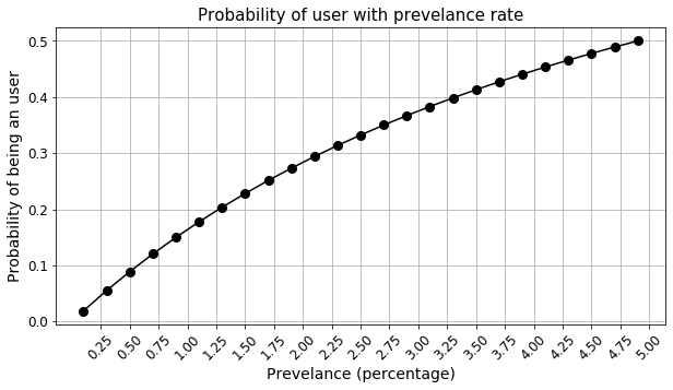
- Note, your decision depends on the probability threshold. Currently, it is set to 0.5. You can lower it if necessary. But, at the threshold of 0.5, you need to have an almost 4.8% prevalence rate to catch a user with a single positive test result.
What level of test capability is needed to improve this scenario?
- We saw that the test sensitivity and specificity impact this computation strongly. So, we may like to see what kind of capabilities are needed to improve the likelihood of catching drug users.


-
The plots above clearly show that even with close to 100% sensitivity, we don’t gain much at all. However, the probability response is highly non-linear with respect to the specificity of the test and as it reaches perfection, we get a large increase in the probability. Therefore, all R&D efforts should be focused on how to improve the specificity of the test.
-
This conclusion can be intuitively derived from the fact that the main issue with having low probability is the low prevalence rate. Therefore, catching non-users correctly (i.e., improving specificity) is the area where we should focus on because they are much larger in numbers than the user.
-
Negative examples are much higher in number than the Positive examples in this problem. Therefore, the True Negative performance of the test should be excellent.
Chaining Bayes’ rule

-
The best thing about Bayesian inference is the ability to use prior knowledge in the form of a Prior probability term in the numerator of the Bayes’ theorem.
-
In this setting of drug screening, the prior knowledge is nothing but the computed probability of a test which is then fed back to the next test.
-
That means, for these cases, where the prevalence rate in the general population is extremely low, one way to increase confidence is to prescribe subsequent test if the first test result is positive.
-
The posterior probability from the first test becomes the Prior for the second test, i.e., the P(user), is not the general prevalence rate anymore for this second test, but the probability from the first test.
-
Here is the simple code for demonstrating the chaining.
p1 = drug_user(prob_th=0.5,sensitivity=0.97,specificity=0.95,prevelance=0.005)
print("Probability of the test-taker being a drug user, in the first round of test, is:",round(p1,3))
print()
p2 = drug_user(prob_th=0.5,sensitivity=0.97,specificity=0.95,prevelance=p1)
print("Probability of the test-taker being a drug user, in the second round of test, is:",round(p2,3))
print()
p3 = drug_user(prob_th=0.5,sensitivity=0.97,specificity=0.95,prevelance=p2)
print("Probability of the test-taker being a drug user, in the third round of test, is:",round(p3,3))
- When we run this code, we get the following,
The test-taker may not be an user
Probability of the test-taker being a drug user, in the first round of test, is: 0.089

The test-taker could be an user
Probability of the test-taker being a drug user, in the second round of test, is: 0.654

The test-taker could be an user
Probability of the test-taker being a drug user, in the third round of test, is: 0.973
-
When we run the test the first time, the output (posterior) probability is low, only 8.9%, but that goes up significantly up to 65.4% with the second test, and the third positive test puts the posterior at 97.3%.
-
Therefore, a test, which is unable to screen a user first time, can be used multiple times to update our belief with the successive application of Bayes’ rule.
The best thing about Bayesian inference is the ability to use prior knowledge in the form of a Prior probability term in the numerator of the Bayes’ theorem.
Summary
-
In this article, we show the basics and application of one of the most powerful laws of statistics — Bayes’ theorem. Advanced probabilistic modeling and inference process that utilizes this law, has taken over the world of data science and analytics in recent years.
-
We demonstrated the application of Bayes’ rule using a very simple yet practical example of drug-screen testing and associated Python code. We showed how the test limitations impact the predicted probability and which aspect of the test needs to be improved for a high-confidence screen.
-
We further showed how multiple Bayesian calculations can be chained together to compute the overall posterior and the true power of Bayesian reasoning.
Further reading
Citation
If you found our work useful, please cite it as:
@article{Chadha2020DistilledBayesTheorem,
title   = {Bayes' Theorem},
author  = {Chadha, Aman},
journal = {Distilled AI},
year    = {2020},
note    = {\url{https://aman.ai}}
}