Primers • Approximate Nearest Neighbors for Similarity Search
- What is Similarity Search?
- Approximate Nearest Neighbors (ANN)
- ANN Algorithms
- ANN Libraries
- Comparative Analysis
- ANN-Benchmarks
- References
- Citation
What is Similarity Search?
- Similarity search is a fundamental computational technique that enables the retrieval of items from a dataset that are most similar to a given query item. Instead of relying solely on exact matches, similarity search evaluates how closely data records resemble each other based on their semantic content. This capability underpins numerous real-world applications across diverse domains.
Real-World Applications
-
In modern machine learning and artificial intelligence systems, similarity search serves as a core component in scenarios such as:
- Image retrieval: Given a sample image, retrieve visually or contextually similar images from a database (e.g., identifying similar fashion items or duplicate product listings).
- Document retrieval: Powering search engines that return semantically relevant documents in response to a textual query.
- Recommendation systems: Suggesting products, movies, or music that align with a user’s preferences by identifying similar users or items.
- Facial recognition and biometric systems: Matching a given face or fingerprint to a stored identity profile.
- Medical imaging: Retrieving similar radiology scans to assist in diagnosis by comparing new cases with historical datasets.
-
These applications share a common requirement: the ability to measure and compare the semantic similarity between high-dimensional data objects such as images, text, audio, or even multi-modal inputs.
From Exact to Approximate Nearest Neighbor Search
-
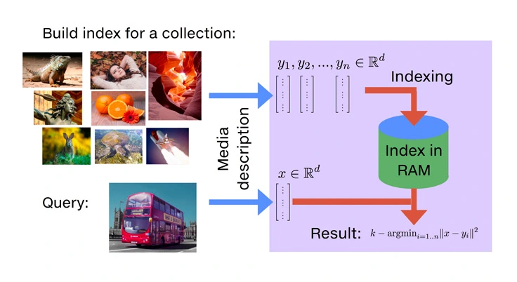
At the heart of similarity search is the concept of nearest neighbor (NN) search. This involves representing each item (e.g., a document, image, or user profile) as a high-dimensional vector using embeddings derived from machine learning models. The task is to find the nearest vectors to a query vector using a defined distance metric, commonly Euclidean distance or cosine similarity.
-
Exact Nearest Neighbor (ENN) search involves scanning all vectors in the dataset to compute distances to the query vector, and then selecting the closest ones. While accurate, this method becomes computationally expensive and inefficient as the dataset size and dimensionality grow.
-
Approximate Nearest Neighbor (ANN) search offers a scalable alternative by sacrificing a small degree of accuracy to achieve significant gains in speed and memory efficiency. ANN methods use specialized data structures and algorithms to rapidly locate vectors that are close to the query vector, without exhaustively comparing all options.
-
This trade-off makes ANN especially valuable in real-time applications where speed and scalability are paramount, such as live recommendation engines or large-scale search systems.
- To compare and evaluate the performance of different ANN methods, practitioners often refer to standardized benchmarks such as ANN-Benchmarks, which test algorithms across datasets and metrics.
- This primer will focus on the exploration of Approximate Nearest Neighbors in greater detail.
Approximate Nearest Neighbors (ANN)
- Approximate Nearest Neighbor (ANN) techniques are crucial for enabling fast and scalable similarity search, especially when working with large, high-dimensional datasets. These methods are designed to retrieve near-optimal neighbors for a query point without the computational overhead of exhaustively comparing against every item in the dataset. By slightly compromising on accuracy, ANN methods dramatically improve search speed and memory efficiency.
Role of ANN in Recommendation Systems
-
ANN methods are widely integrated into modern recommender systems to complement or enhance traditional collaborative and content-based filtering. Their utility arises from addressing several limitations of classical approaches, particularly in large-scale or real-time environments. To understand their impact more concretely, consider how ANN techniques address four critical challenges in recommender system design: scalability, latency, diversity, and the cold start problem:
-
Scalability: Collaborative filtering and content-based filtering often require computing pairwise similarity between large numbers of users or items. As datasets grow to millions or billions of records, this becomes computationally infeasible using exact methods. ANN techniques introduce indexing and search strategies that scale sub-linearly with dataset size, enabling efficient candidate generation for downstream ranking stages.
-
Real-Time Recommendation: In user-facing applications, recommendations must often be served in milliseconds. ANN algorithms support low-latency query execution, making them suitable for real-time contexts such as e-commerce search, streaming media recommendations, and social media feeds. By pre-indexing the dataset and optimizing search traversal, ANN methods ensure timely responses without compromising system throughput.
-
Diversity and Serendipity: One downside of traditional filtering techniques is their tendency to recommend highly similar items, which can lead to filter bubbles. ANN allows recommender systems to retrieve a broader and more diverse candidate pool by identifying not only the closest items but also those within a proximity threshold. This promotes user engagement through serendipitous discoveries while still respecting personalization constraints.
-
Cold Start Handling: When new users or items are introduced to the system, classical models often lack sufficient interaction data to generate accurate recommendations. ANN methods help mitigate the cold start problem by leveraging metadata or embedding vectors derived from auxiliary data (e.g., textual descriptions, visual content). These embeddings can be used to identify similar existing users or items, facilitating meaningful initial recommendations.
-
-
By integrating ANN techniques into recommender architectures, systems achieve enhanced scalability, responsiveness, recommendation diversity, and robustness to data sparsity—all critical for modern, dynamic applications.
ANN Algorithms
- ANN search is underpinned by a range of algorithmic strategies designed to support scalable, high-speed querying in high-dimensional spaces. These algorithms are broadly grouped into graph-based, tree-based, quantization-based, and clustering-based families. Each comes with specific implementation considerations, data structures, and optimization techniques.
- The ANN algorithms below have been sorted from simplest to most complex based on their underlying strategy types—starting with tree-based methods (e.g., KD-Tree, Annoy), followed by quantization-based methods (e.g., PQ, OPQ), clustering-based methods (e.g., IVF, RVQ), and finally graph-based methods (e.g., HNSW, FINGER) in the later rows.
Tree-Based Methods
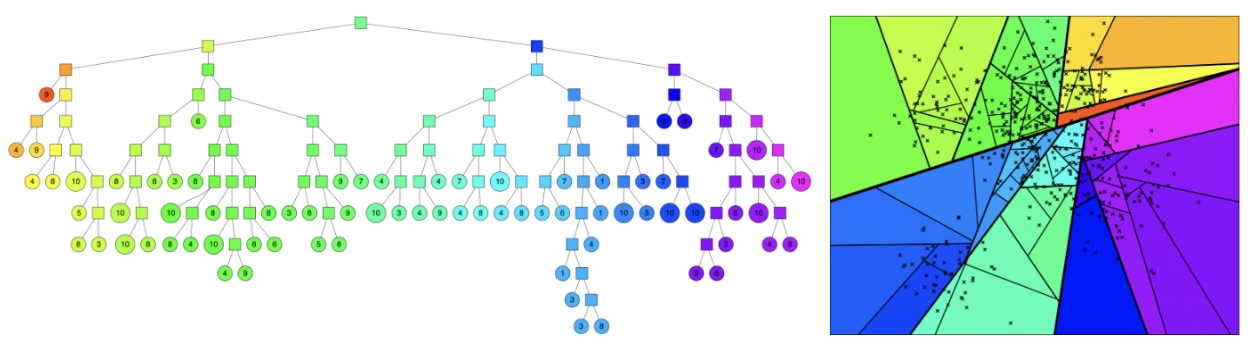
- Tree-based methods form one of the earliest and most widely adopted strategies for nearest neighbor search. They operate by recursively dividing the vector space using hyperplanes (such as axis-aligned or randomly oriented splits), resulting in hierarchical structures like binary trees or forests. During querying, these structures enable the algorithm to efficiently prune large portions of the search space, reducing the number of distance computations required.
-
In real-world scenarios, tree-based methods are frequently used in settings where:
- Dimensionality is moderate (typically under 100 dimensions), and datasets are either static or change infrequently.
- Speed and interpretability are critical, such as in robotics, computer vision, and industrial inspection systems, where tree traversal paths can be inspected or constrained.
- Low-latency and real-time processing is required, such as in SLAM (Simultaneous Localization and Mapping), object recognition in AR/VR applications, or drone navigation systems, where rapid approximate lookups are essential.
- Embedded or resource-constrained environments are involved, where lightweight in-memory or file-based indices (as supported by Annoy) are more suitable than GPU-intensive solutions.
- Tree-based methods also serve as foundational components in hybrid pipelines—often combined with graph-based or quantization-based modules to accelerate coarse filtering before refined re-ranking stages.
- Despite their limitations in high-dimensional contexts, their speed, simplicity, and practical effectiveness make them a valuable tool in many production-grade systems.
KD-Trees
-
Partition Strategy: Recursive binary splits along dimensions with maximum variance.
-
Search:
- Traverses down the tree to a leaf.
- Backtracking is used to check sibling branches when necessary.
-
Implementation:
- Fast for dimensions < 30.
- Can use priority queues to simulate best-first search.
- Common in libraries like FLANN (Fast Library for Approximate Nearest Neighbors).
-
Pros:
- Simple and interpretable structure.
- Low memory overhead.
- Fast for low-dimensional, static datasets.
-
Cons:
- Performance degrades rapidly in high-dimensional spaces.
- Not suitable for dynamic datasets or frequent updates.
-
Use Case:
- KD-Trees are suited for structured and low-dimensional datasets such as geospatial data, robotics, and image metadata. They are widely used in scientific computing and real-time systems requiring deterministic and interpretable behavior. They’re ideal for exact or nearly exact queries in small- to medium-sized vector collections.
Randomized KD-Forests
-
Multiple KD-Trees: Built with randomized split choices or axis shuffling.
-
Search:
- Queries traverse multiple trees in parallel.
- Results from all trees are merged.
-
Parameters:
n_trees: Number of trees to build (impacts accuracy and index size).leaf_size: Minimum number of items in leaf nodes.search_checks: Max nodes visited during querying.
-
Pros:
- Improves robustness over standard KD-trees.
- Offers tunable accuracy-speed trade-offs.
- Better suited to moderate dimensionality (up to ~100 dimensions).
-
Cons:
- Higher memory footprint due to multiple trees.
- Requires careful tuning to avoid overfitting or redundancy.
- Performance still degrades in high-dimensional regimes.
-
Use Case:
- Randomized KD-Forests are effective in handling medium-scale datasets where standard KD-trees fail due to dimensionality. They’re often used in real-time search applications like 3D point cloud matching and visual SLAM in robotics, offering a balance between accuracy and responsiveness.
Annoy’s Random Projection Forest
-
Partition Strategy:
- Randomly select two points, compute their midpoint hyperplane, and recursively partition the dataset.
-
Index:
- A forest of such trees is constructed.
- Each tree introduces different hyperplane splits, improving diversity.
-
Search:
- Each tree yields a list of candidate points.
- Combined and sorted using brute-force on small candidate sets.
-
File-based Indexing:
- Indexes saved to disk as static files and memory-mapped at query time.
- Efficient for multi-process access and low RAM environments.
-
Pros:
- Memory-efficient via on-disk index loading.
- Supports shared access across processes.
- Simple to implement and tune (
n_trees,search_k).
-
Cons:
- Index is static—no support for incremental updates.
- Lacks GPU and batch processing support.
- Recall suffers at high dimensionality or when optimal tree coverage is hard to achieve.
-
Use Case:
- Annoy is used extensively in static recommendation systems, such as music and content suggestion engines (e.g., Spotify). Its design favors read-heavy workloads, and it’s especially effective when indexes must be shared across processes or run in constrained environments like embedded systems.
Quantization-Based Methods
-
Quantization-based methods are built on the idea of compressing high-dimensional vectors into compact, lossy representations, typically by mapping them to a discrete set of centroids or codes. These compact codes allow extremely fast approximate distance computation using precomputed lookup tables, making them ideal for billion-scale vector search tasks.
-
These methods are widely used in industry for:
- Large-scale image/video/text retrieval where space and speed are at a premium.
- Real-time inference pipelines that need rapid ranking of semantically similar results.
- Hybrid ANN pipelines, often paired with clustering (IVF) or re-ranking modules.
- Scenarios that require deployment on limited-memory devices or optimized GPU environments.
-
Despite their reliance on lossy compression, modern quantization approaches (e.g., OPQ, AVQ) offer a high degree of accuracy, particularly when tuned carefully.
Product Quantization (PQ)
-
Overview:
- Vector
xis split intomsub-vectors. - Each sub-vector is quantized into one of
kcentroids (learned using k-means). - Final code is a tuple of centroid indices.
- Vector
-
Search:
- Precompute a distance table for each query sub-vector and all subspace centroids.
- Final distance is the sum of subspace distances from lookup tables.
-
Implementation:
- In FAISS, PQ is implemented with SIMD intrinsics and fused operations.
- Typically used with IVF (Inverted File Index) for additional speed-up.
-
Pros:
- Excellent compression with minimal storage cost.
- Efficient for both CPU and GPU architectures.
- Fast distance computation using lookups, no full vector arithmetic needed.
-
Cons:
- Sensitive to data distribution; uniform quantization can lose detail.
- May degrade recall for fine-grained queries or tightly clustered data.
-
Use Case:
- PQ is commonly used in large-scale image and video retrieval systems. It’s a standard method in FAISS-based deployments at billion-scale for deduplication, facial recognition, and fast similarity ranking in content libraries, where compact representation is essential.
Optimized Product Quantization (OPQ)
-
Extension to PQ:
- Learn a rotation matrix to decorrelate input vectors before PQ encoding.
- Reduces quantization loss, improving accuracy.
-
Training:
- Alternates between PCA-like optimization and quantization.
- Computationally heavier but yields significant accuracy improvements.
-
Pros:
- Lower distortion than basic PQ, especially for high-dimensional, correlated data.
- Flexible, modular integration with other indexing structures (e.g., IVF).
-
Cons:
- Slower training and more complex parameter tuning.
- Requires retraining if the data distribution shifts significantly.
-
Use Case:
- OPQ is deployed in precision-sensitive search scenarios such as e-commerce or financial recommendation systems, where even small gains in accuracy translate to meaningful impact. It’s ideal for embedding pipelines where dimension correlations hurt performance.
Locality Sensitive Hashing (LSH)
-
Hashing Scheme:
- Family of hash functions ensures that similar vectors hash to the same bucket with high probability.
- For cosine similarity: random hyperplane hash functions.
-
Multi-Probe LSH:
- During query, multiple nearby buckets are probed to improve recall.
-
Challenges:
- Works best for low to moderate dimensions.
- Often memory-intensive and suffers in high-density regions of vector space.
-
Pros:
- Extremely fast sublinear search; constant-time hash lookups.
- Simple to implement with theoretical performance guarantees.
-
Cons:
- Poor recall for complex, high-dimensional datasets.
- High memory usage for large numbers of hash tables.
- Tuning hash functions and probing depth is non-trivial.
-
Use Case:
- LSH is suitable for real-time systems with strict latency requirements, such as fraud detection, duplicate detection, or real-time alerting, where a fast but approximate match is preferable to delayed precision.
Anisotropic Vector Quantization (AVQ)
-
Used in ScaNN:
- Unlike PQ, AVQ allows the shape of quantization cells to adapt to the data distribution.
- Each centroid has an anisotropic (elliptical) region rather than spherical.
-
Index Construction:
- Uses SVD-like analysis to deform Voronoi cells.
- Quantization boundaries are optimized to better reflect real data spread.
-
Search:
- Improves Maximum Inner Product Search (MIPS) accuracy by focusing on high-value candidates.
-
Pros:
- Adapts well to non-uniform data densities.
- Superior recall in semantic search applications compared to isotropic quantizers.
- Well-suited to modern ML-generated embeddings.
-
Cons:
- More complex to construct and train than standard PQ.
- Not yet widely supported outside of ScaNN.
- Longer index build time due to centroid deformation.
-
Use Case:
- AVQ is tailored for semantic search tasks in NLP and vision systems, where embedding density varies. It powers systems like ScaNN that handle document retrieval, passage re-ranking, or intent classification using deep-learned embeddings.
Clustering-Based Methods
- Clustering-based approaches are a foundational class of ANN algorithms that partition the dataset into discrete groups or clusters using unsupervised learning techniques, most commonly k-means. These clusters serve as coarse partitions of the search space, enabling fast and scalable nearest neighbor search by reducing the number of direct comparisons required at query time.
-
Clustering-based methods are particularly effective when used as the first stage in multi-step retrieval architectures. They are often combined with quantization and re-ranking techniques to build high-performance ANN systems for web-scale search and recommendation. Each of these clustering-based approaches is most effective when integrated into layered ANN architectures. For example:
- FAISS IVF-PQ: Combines IVF for coarse partitioning with PQ for fine-grained, compressed distance approximation.
- ScaNN: Employs k-means-style partitioning trees with AVQ and late-stage re-ranking.
- Two-Stage Retrieval Systems: Use clustering to shortlist candidates and exact scoring for ranking.
Inverted File Index (IVF)
-
Partition Strategy:
- The dataset is partitioned using k-means clustering into
nlistcoarse centroids. Each data point is assigned to its nearest centroid, forming an inverted list for that cluster.
- The dataset is partitioned using k-means clustering into
-
Search:
- At query time, the query vector is compared to all centroids, and the top
nprobeclosest centroids are selected. - Only the vectors in the selected clusters are searched, significantly narrowing down the search space.
- At query time, the query vector is compared to all centroids, and the top
-
Index Construction:
- A training phase precedes indexing, where representative centroids are learned from a sample of the dataset.
- Vectors are then indexed into inverted lists corresponding to their nearest centroid.
-
Implementation:
- IVF is commonly used in combination with Product Quantization (e.g., IVF-PQ in FAISS) to compress vectors and reduce memory usage while maintaining retrieval performance.
-
Pros:
- Scalable to billions of vectors.
- Fast query execution due to aggressive pruning.
- Integrates well with quantization and re-ranking modules.
-
Cons:
- Requires careful tuning of
nlist(cluster count) andnprobe(clusters to scan at query time). - Clustering quality impacts recall and precision.
- Requires careful tuning of
-
Use Case:
- Powers large-scale similarity search in systems such as Facebook’s visual search infrastructure and semantic embedding-based recommendation engines. Widely deployed in FAISS IVF-PQ and hybrid indexing pipelines.
Residual Vector Quantization (RVQ)
-
Overview:
- RVQ recursively encodes a vector by applying multiple layers of quantization, each capturing the residual error left by the previous layer.
- This hierarchical structure allows for progressively finer approximations of the original vector.
-
Search:
- Queries are encoded using the same residual structure and matched against compound codes generated during indexing.
- Suitable for scenarios where single-code quantization (as in PQ) fails to preserve sufficient detail.
-
Index Construction:
- Involves training multiple codebooks sequentially, each learning to quantize the residual of the prior stage.
- Typically implemented in vector search systems that require higher recall than basic PQ can offer.
-
Pros:
- Delivers better accuracy than single-pass quantization.
- Supports fast computation with table lookups and SIMD-accelerated operations.
-
Cons:
- More complex to train and tune.
- Increased query-time latency due to deeper decoding stages.
-
Use Case:
- Used in high-recall scenarios such as document retrieval, legal and biomedical search engines, and advanced FAISS configurations where accuracy is prioritized over absolute speed.
Scalable K-Means Clustering (Mini-Batch K-Means)
-
Purpose:
- Designed to handle clustering on very large datasets by using small, randomly selected subsets (mini-batches) for iterative updates.
- Enables efficient, online construction of cluster centroids without processing the entire dataset at once.
-
Search Integration:
- Frequently used to generate cluster centroids in IVF-like indexing schemes or to enable dynamic re-clustering of streaming data.
-
Training Efficiency:
- Orders of magnitude faster than traditional k-means for large datasets.
- Supports continual training or incremental centroid updates.
-
Pros:
- Suitable for massive datasets that exceed memory constraints.
- Faster training with minimal accuracy loss compared to full-batch methods.
-
Cons:
- Quality of clusters depends on batch size and sampling strategy.
- Can converge to suboptimal centroids in non-uniform or complex vector distributions.
-
Use Case:
- Ideal for dynamic or streaming data environments, such as online recommendation platforms, personalization systems, or large-scale ad retrieval where vector distributions evolve over time.
Graph-Based Methods
-
Graph-based methods construct navigable proximity graphs where each node represents a data point and edges connect it to a selection of its approximate nearest neighbors. These methods enable efficient similarity search through greedy traversal, allowing the system to reach relevant regions of the data space without exhaustively scanning all vectors.
-
These algorithms are especially effective in high-dimensional spaces where traditional methods struggle. They are widely used in real-world systems because of:
- Excellent accuracy-speed trade-offs, particularly at high recall thresholds.
- Support for dynamic updates, which is crucial for evolving datasets.
- High empirical performance across embedding types (text, image, video, audio).
- Adoption in commercial-grade vector databases and search systems, including Vespa, Milvus, Weaviate, Pinecone, and OpenSearch extensions.
-
Applications include semantic search, recommendations, online personalization, ad retrieval, fraud detection, and large-scale analytics.
Navigable Small Worlds (NSW)
-
NSW is a foundational graph-based ANN algorithm that constructs a proximity graph without hierarchical layers, relying instead on local navigation and randomized connectivity to explore the data space.
-
Data Structure: A single-layer navigable graph where each node is connected to a subset of its nearest neighbors based on proximity.
-
Construction:
- Nodes are added one by one using randomized greedy strategies.
- For each new node, a set of connections is formed to existing nodes that are closest in terms of distance.
- Edge formation favors a small-world topology: short paths exist between any two nodes, enabling quick traversal.
-
Search:
- Begins at a randomly selected node.
- Follows a greedy walk, moving to the neighbor closest to the query.
- Terminates once no neighbor is closer than the current node—reaching a local optimum.
-
Pros:
- Straightforward to implement and debug.
- Requires minimal configuration—fewer hyperparameters than hierarchical models.
- Lower memory usage than multilayer graphs.
-
Cons:
- No hierarchical navigation; search can be slower or less reliable.
- Convergence to the global nearest neighbor is not guaranteed.
- Less suited for very large datasets or high-recall applications.
-
Use Case:
- NSW is best suited for simpler, smaller-scale applications or environments with limited computational resources. Common in research settings, educational tools, or embedded systems where a lightweight ANN solution is needed.
Fast Inference for Graph-Based ANN (FINGER)
-
FINGER is a graph search optimization that accelerates nearest neighbor search by reducing the number of exact distance computations during traversal.
-
Algorithmic Enhancement:
- FINGER is not a standalone graph algorithm but a technique that enhances existing graph-based methods such as NSW or HNSW.
-
Technique:
- Decomposes vectors into components (projections and residuals).
- Estimates distances using angular relationships and dot products.
- Avoids costly full-vector comparisons for less promising candidates.
-
Integration:
- Applied exclusively at query time.
- Does not alter the underlying graph; can be used on top of existing indexes.
- Particularly beneficial for large graphs with dense connectivity.
-
Pros:
- Reduces search latency by 20–60% in practice.
- Easy to integrate without retraining or rebuilding the index.
- Compatible with both simple (NSW) and hierarchical (HNSW) graphs.
-
Cons:
- Performance gains vary with data characteristics (e.g., vector distribution).
- Adds complexity to the search logic.
- May slightly reduce recall if approximation is too aggressive.
-
Use Case:
- FINGER is ideal for latency-critical applications such as real-time recommendations, search-as-you-type interfaces, and live personalization systems. It helps accelerate existing HNSW or NSW graphs without requiring structural changes.
Hierarchical Navigable Small Worlds (HNSW)
-
HNSW is a state-of-the-art ANN graph algorithm that improves upon NSW by introducing a hierarchical structure and multiple levels of graph connectivity.
-
Data Structure:
- A multilayer graph in which higher levels connect long-range links and lower levels represent local neighborhoods.
- Nodes appear at multiple levels, with decreasing density as the level increases.
-
Construction:
- Each point is assigned a random maximum layer.
- Insertions start at the top and descend layer by layer, connecting to the closest nodes at each level.
- Parameters like
M(max edges per node) andefConstructioncontrol connectivity.
-
Search:
- Starts from the topmost layer using a greedy search.
- Progressively moves down levels, narrowing the search to increasingly local areas.
efSearchdetermines the number of nodes visited during querying.
-
Implementation Notes:
- Well-optimized in libraries such as NMSLIB, FAISS, and hnswlib.
- Supports dynamic insertions and deletions, making it suitable for production systems.
-
Pros:
- Achieves high recall at low latency.
- Scales efficiently to millions of high-dimensional vectors.
- Tunable for different performance requirements.
- Robust in both static and dynamic settings.
-
Cons:
- Higher memory usage due to multilayer structure.
- Longer index build times, especially with large datasets.
- Requires hyperparameter tuning for optimal performance.
-
Use Case:
- HNSW is the industry-standard graph-based ANN algorithm used in high-performance vector search platforms. It powers semantic retrieval in document search, personalized content feeds, similarity-based product recommendation, and large-scale embedding search in databases like Vespa, Weaviate, and Pinecone.
Tabular Comparison
| Algorithm | Data Structure | Construction Strategy | Search Strategy | Key Strengths | Limitations |
|---|---|---|---|---|---|
| Tree-Based Methods | |||||
| KD-Tree | Binary tree with axis-aligned splits | Recursive partitioning along max-variance axes | Tree traversal with backtracking | Fast for low dimensions (<30), simple structure | Degrades in high-dimensional spaces |
| Randomized KD-Forest | Multiple KD-Trees with random splits | Parallel tree building with randomized axes | Aggregate candidates from all trees | Improved recall over single KD-tree | Higher memory and tuning complexity |
| Annoy Forest | Forest of binary trees via random projections | Random hyperplane splits | Tree-wise candidate extraction with brute-force refinement | Memory-mapped files, low RAM use, fast lookup | Static index, no GPU/batch support |
| Quantization-Based Methods | |||||
| Product Quantization (PQ) | Codebooks for each subspace of vector | K-means on vector subspaces | Lookup-table based distance approximation | Compact codes, efficient on CPUs/GPUs | Accuracy loss due to quantization |
| Optimized PQ (OPQ) | Rotated subspace codebooks | Learned rotation + PQ training | Same as PQ, with lower quantization error | Better accuracy than PQ, widely supported | Heavier training, complex tuning |
| Clustering-Based Methods | |||||
| Inverted File Index (IVF) | Cluster centroids with inverted lists | k-means clustering for coarse partitioning | Select nearest clusters and search within them | Scalable to billions of vectors, integrates with quantization | Clustering quality impacts recall and precision |
| Residual Vector Quantization (RVQ) | Hierarchical residual codebooks | Recursive quantization of residuals | Multi-stage decoding and comparison | Higher recall than single-level quantizers | Increased query latency, complex training |
| Mini-Batch K-Means | Incrementally updated cluster centroids | Iterative mini-batch updates on sampled data | Used to assign points or create IVF partitions | Efficient training on large datasets, supports streaming data | Cluster quality depends on batch configuration |
| Graph-Based Methods | |||||
| NSW | Single-layer navigable small-world graph | Randomized edge insertion based on proximity | Greedy walk guided by local nearest neighbors | Lightweight, easy to implement, lower memory | No hierarchy, slower convergence, reduced recall in complex data |
| FINGER | Augmentation over navigable graph | No structural changes; integrates into search phase | Approximate distance estimation via vector projections | Accelerates search in existing graphs, reduces computation by 20–60% | Dependent on vector distribution, adds search-time complexity |
| HNSW | Multilayer navigable proximity graph | Greedy layer-wise insertion with long- and short-range links | Hierarchical greedy search with priority queue | High recall, dynamic updates, excellent accuracy-speed trade-off | High memory usage, longer build time, parameter tuning required |
Choosing the right ANN algorithm family
-
Here’s a guide to help you choose the right ANN algorithm family based on your data characteristics and application requirements:
-
Tree-Based Methods (KD-Tree, Randomized KD-Forest, Annoy): These methods shine when your vectors live in low to moderate dimensions (roughly up to 100), and you need interpretable, lightweight indices that rarely change. They’re ideal for static or slowly evolving datasets where you can afford occasional full-index rebuilds. Use them in robotics or AR/VR for real-time pose estimation and mapping, in embedded recommendation systems with tight memory budgets, or whenever you want deterministic search paths you can debug or constrain.
-
Quantization-Based Methods (PQ, OPQ, LSH, AVQ): If you’re dealing with millions or billions of high-dimensional embeddings and need extreme compression without sacrificing too much accuracy, quantization is your go-to. Product Quantization (PQ) and its optimized variant (OPQ) deliver compact codes and very fast lookups on CPU or GPU, perfect for large-scale image/video retrieval or e-commerce rankers. Locality Sensitive Hashing (LSH) works best when you need sub-millisecond lookups and can tolerate lower recall, as in fraud detection or duplicate alerting. Anisotropic Vector Quantization (AVQ) is a niche choice when embedding distributions vary wildly and you need better recall than PQ can offer—common in semantic search with neural embeddings.
-
Clustering-Based Methods (IVF, RVQ, Mini-Batch K-Means): Use clustering to get a coarse shortlist before applying fine-grained search. IVF (often paired with PQ) scales to web-scale collections by scanning only a few inverted lists, making it the backbone of billion-vector systems like FAISS deployments. If you need higher recall than PQ-only pipelines, Residual Vector Quantization (RVQ) provides deeper approximation at the cost of slightly higher query latency. For streaming or dynamic data where clusters must evolve over time, Mini-Batch K-Means lets you update centroids online with minimal compute.
-
Graph-Based Methods (NSW, FINGER, HNSW): When your vectors are very high-dimensional and you demand both high recall and low latency—especially in dynamic settings—graph methods dominate. Hierarchical Navigable Small Worlds (HNSW) offers state-of-the-art accuracy-speed trade-offs and supports incremental updates, making it the de facto choice in production vector databases and semantic search engines. If you already have an HNSW or NSW graph and need to shave off extra microseconds at query time, apply FINGER on top to reduce exact distance computations. For smaller or research-oriented setups where simplicity matters, pure NSW can be a lightweight starting point.
-
-
Choose based on your primary constraints—dimensionality, scale, update frequency, memory footprint, latency budget, and accuracy targets. Mixing families (for example, IVF-PQ or tree pre-filtering before a graph search) often yields the best balance in large-scale, production ANN pipelines.
ANN Libraries
- While ANN algorithms provide the foundational theory for efficient similarity search, their widespread use in real-world applications is made possible by powerful open-source libraries. These libraries abstract away the low-level implementation details and offer optimized, production-ready APIs for indexing, querying, and evaluating high-dimensional data.
- Below, we examine three leading libraries: FAISS, ScaNN, and ANNOY.
FAISS (Facebook AI Similarity Search)
- FAISS is a highly optimized C++ library with Python bindings, developed by Facebook AI Research to support efficient similarity search over large-scale datasets of dense vectors. It is widely used in both academic research and industrial systems.
Key Features
-
Multiple Indexing Strategies:
- Flat Index: Exhaustive search for exact results.
- Inverted File Index (IVF): Partitions data using k-means centroids; search occurs in the closest partitions.
- Product Quantization (PQ) and Optimized PQ (OPQ): Compresses vectors into compact codes.
- IVF-PQ/IVF-OPQ: Combines inverted indexing with quantization for speed-accuracy trade-offs.
- HNSW: Integrated for graph-based search.
-
GPU Acceleration:
- FAISS provides CUDA-based implementations for key indexing methods.
- Enables real-time search on billion-scale datasets.
-
Scalability:
- Supports distributed indexing using sharding.
- Can operate on datasets that do not fit into RAM using memory-mapped files.
Search Workflow
- Training: For PQ or IVF, the index must first be trained on a representative sample.
- Indexing: Vectors are added to the index using
.add()or.add_with_ids(). - Querying: The
.search()method returns the k nearest neighbors for each query. - Tuning: Parameters like
nlist(number of clusters),nprobe(number of partitions to search), and PQ code size significantly affect accuracy and speed.
Evaluation Metrics
- Speed: Number of queries per second or average query latency.
- Memory Usage: Especially critical when using PQ or GPU mode.
- Accuracy: Measured using recall metrics (e.g., recall\@1, recall\@10).
Pros
- High flexibility and modular design.
- GPU acceleration with multi-threaded CPU support.
- Rich suite of index types and hybrid approaches.
Cons
- Can be complex to configure optimally.
- GPU integration requires familiarity with CUDA.
- No built-in support for dynamic (online) index updates; best suited for batch ingestion.
ScaNN (Scalable Nearest Neighbors)
- ScaNN is an efficient similarity search library developed by Google Research, tailored for Maximum Inner Product Search (MIPS) and high-accuracy ANN in embedding-based retrieval systems.
Key Features
-
Hybrid Indexing Architecture:
- Partitioning Tree: Efficiently narrows the candidate set using k-means clustering or partition trees.
- Asymmetric Distance Computation (ADC): For fast dot-product or Euclidean similarity.
- Anisotropic Vector Quantization (AVQ): Optimized for high-dimensional and non-uniform data, offering more accurate and balanced indexing.
Anisotropic Vector Quantization (AVQ)
-
Anisotropic Vector Quantization (AVQ) is a core indexing technique used in ScaNN to enhance performance in real-world, high-dimensional datasets. AVQ is specifically designed for anisotropic distributions, where vector densities vary significantly across the embedding space.
-
Quantization Grid:
- AVQ begins by dividing the space into a grid of quantization cells. Each cell corresponds to a cluster of vectors grouped by proximity under Euclidean distance.
-
Anisotropic Adjustment:
- Unlike standard product quantization, AVQ adapts the shape and size of each grid cell to reflect the local density and orientation of the data.
- This is achieved via transformations that deform cells based on principal directions, producing elliptical (rather than spherical) boundaries.
-
Indexing Phase:
- During index construction, vectors are assigned to their nearest quantization cell using modified centroids.
- This mapping improves clustering accuracy, especially in regions where traditional uniform quantization fails.
-
Search Phase:
- For a given query, ScaNN identifies the most relevant cells and retrieves candidate vectors.
- These candidates are further refined through re-ranking using higher-precision computations, typically involving dot products or exact distances.
-
Performance Benefits:
- AVQ significantly reduces the number of comparisons by focusing the search on well-shaped regions of the vector space.
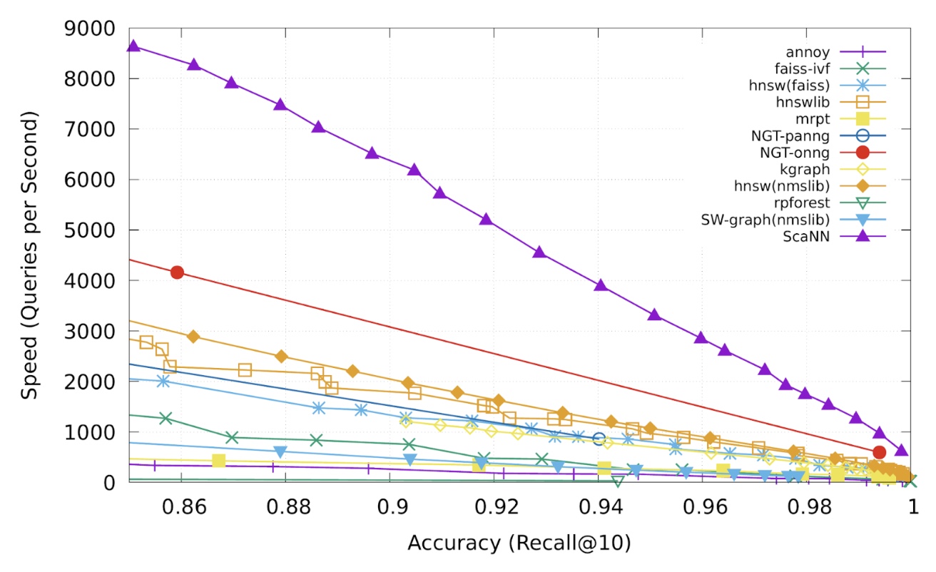
- On benchmarks like glove-100-angular, ScaNN has demonstrated superior performance, handling nearly twice the query load at the same accuracy compared to the next-best library (NGT-onng).
- This quantization method is especially useful in deep learning workloads where embeddings exhibit high variance in density.
Use Case: Semantic Search
- ScaNN excels in use cases where embeddings are generated from text, images, or product metadata using deep learning models. Its design is aligned with the two-tower model, where both queries and items are independently embedded into a shared vector space.
Implementation Considerations
- Training: Required for quantization and partitioning.
- Search Configuration: Parameters such as the number of clusters, quantization depth, and number of re-ranked results need tuning.
- Deployment: Can be used with TensorFlow Serving or directly integrated into a backend service.
- ScaNN is open-source and available via GitHub. It can be installed via Pip and supports both TensorFlow and NumPy inputs.
Pros
- High accuracy and throughput for MIPS.
- Strong performance on semantically rich embeddings.
- Open-source and actively maintained.
Cons
- Less mature ecosystem than FAISS.
- GPU support is limited.
- Initial index build time can be high.
ANNOY (Approximate Nearest Neighbors Oh Yeah)
- Developed by Spotify, ANNOY is a lightweight and efficient C++ library with Python bindings for performing fast similarity search using random projection forests. It is particularly suitable for static datasets and read-heavy workloads.
Key Features
-
Indexing Method:
- Constructs multiple binary trees using random hyperplane splits.
- Each tree represents a different partitioning of the space.
-
Memory Mapping:
- Indexes are written to disk and memory-mapped at query time.
- Enables extremely fast lookups with minimal RAM usage.
-
Runtime Parameters:
n_trees: Affects accuracy and index size. More trees = better recall.search_k: Controls number of nodes checked during search. Higher values = better accuracy, slower speed.
Use Case: Music Recommendation
- Spotify uses ANNOY for fast retrieval of similar songs, playlists, or users based on vector representations of user behavior or audio features.
Implementation Notes
- Static indexing: Does not support dynamic insertions (though
annoy2aims to address this). - No GPU support.
- No native batch processing interface; needs custom implementation for throughput optimization.
Pros
- Simple to use and highly portable.
- Memory-efficient due to disk-based index.
- Suitable for multi-process environments.
Cons
- Limited support for dynamic updates.
- Slower than FAISS or ScaNN for very large datasets.
- No GPU acceleration or quantization techniques.
- These libraries encapsulate the most widely adopted implementations of ANN techniques in industry today. Each has a different performance profile and is better suited to specific use cases:
- FAISS: Ideal for large-scale, high-performance search with GPU support.
- ScaNN: Excellent for semantically meaningful embeddings and MIPS-heavy workloads.
- ANNOY: Lightweight and efficient for static, read-optimized systems.
Comparative Analysis
-
This section offers a comparison that highlights the fundamental trade-offs between speed, accuracy, memory efficiency, hardware requirements, and integration complexity across major ANN methods and libraries. The most appropriate method depends on factors such as:
-
Dataset Characteristics:
- Size (thousands to billions of vectors)
- Dimensionality (sparse vs. dense vectors, 32–1000+ dimensions)
- Distribution (uniform vs. clustered or anisotropic)
- Update frequency (static vs. dynamic/real-time ingestion)
-
Performance Needs:
- Latency requirements (real-time systems vs. batch recommendations)
- Throughput (queries per second in multi-user environments)
- Index build time and preprocessing overhead
-
Resource Constraints:
- Available memory (RAM vs. disk)
- Compute acceleration (CPU-only vs. GPU-accelerated systems)
- Infrastructure for deployment (cloud-native vs. embedded use cases)
-
Accuracy Tolerance:
- Use cases that demand precise retrieval vs. tolerable approximation
- Top-k recall metrics, precision trade-offs
Tabular Comparison
| Library | Definition/Functioning | Pros | Cons |
|---|---|---|---|
| FAISS | Modular similarity search library supporting flat (brute-force), inverted file (IVF), product quantization (PQ), optimized PQ (OPQ), and graph-based (HNSW) indexing. Offers strong support for hybrid strategies and CUDA-based GPU acceleration. |
|
|
| ScaNN | Google's ANN framework optimized for Maximum Inner Product Search (MIPS). Uses hybrid strategies: tree-based partitioning, anisotropic vector quantization (AVQ), and re-ranking with exact computation. Especially well-suited for semantic embeddings. |
|
|
| ANNOY | Tree-based approach using multiple random projection trees. Each tree splits the space using randomly selected hyperplanes. Designed to trade off build time and search accuracy with minimal memory overhead using memory-mapped files. |
|
|
-
This comparison should guide you toward the best ANN system for your specific technical needs:
- Choose FAISS for large-scale indexing with advanced GPU acceleration and tight performance tuning.
- Use ScaNN if you’re operating on semantic embeddings or deep learning pipelines, particularly with MIPS.
- Opt for ANNOY when working with static datasets in constrained memory environments or needing file-based deployment.
- Prefer HNSW when low latency and high recall are critical, and memory usage is acceptable.
- Consider FINGER as a low-overhead performance enhancer if you already employ graph-based indexes.
ANN-Benchmarks
- ANN-Benchmarks is an open-source benchmarking platform that provides a standardized and reproducible environment for evaluating the performance of approximate nearest neighbor algorithms. It enables researchers and practitioners to assess trade-offs between speed, accuracy, and memory usage across various libraries and algorithmic approaches.
Purpose and Scope
- The benchmark suite is designed to answer key questions such as:
- Which ANN method offers the best speed/accuracy trade-off for a particular type of data?
- How do different libraries perform under the same distance metric?
- What is the relative performance of quantization vs. graph-based indexing on benchmark datasets?
Key Features
-
Common Datasets:
- Includes real-world and synthetic datasets like
SIFT,GloVe,Fashion-MNIST, andDeep Image Descriptors. - Each dataset varies in dimensionality, density, and semantics, allowing for broad evaluation.
- Includes real-world and synthetic datasets like
-
Distance Metrics:
- Supports various metrics such as Euclidean distance (L2), angular distance (cosine similarity), and inner product (for MIPS scenarios).
-
Evaluation Metrics:
- Recall@\(k\): Measures the fraction of true nearest neighbors found in the top-k results.
- QPS (Queries per second): Throughput of the method, showing speed under load.
- Index size and build time: Assesses memory footprint and pre-processing requirements.
-
Leaderboard Interface:
- Live comparison of algorithmic results across datasets.
- Interactive plots showing recall vs. query time, making it easy to identify optimal configurations.
Using ANN-Benchmarks
The benchmarks can be run locally via Docker and Python, allowing users to test their own ANN implementations or configurations. It supports integrating custom methods into the benchmarking pipeline, which makes it a valuable research tool.

Practical Use Cases
- Model Selection: Choose the best ANN library for your specific task and hardware constraints.
- Algorithm Tuning: Understand how hyperparameters like
nlist,nprobe, orsearch_kaffect real-world performance. - Regression Testing: Evaluate how updates to ANN methods impact speed or recall.
References
- Jegou, Hervé, et al., FAISS: A library for efficient similarity search, Engineering at Meta, 29 March 2017.
- Erik Bernhardsson, Efficient Indexing of Billion-Scale datasets of deep descriptors, 1 October 2015.
- Announcing ScaNN: Efficient Vector Similarity Search
- Nearest neighbors and vector models – part 2 – algorithms and data structures
- More-efficient approximate nearest-neighbor search
Citation
If you found our work useful, please cite it as:
@article{VatsChadha2020DistilledApproximateNearestNeighbors,
  title   = {Approximate Nearest Neighbors -- Similarity Search},
  author  = {Chadha, Aman and Jain, Vinija},
  journal = {Distilled AI},
  year    = {2022},
  note    = {\url{https://aman.ai}}
}