Multimodal Machine Learning • Introduction

• Introduction
• Unimodal Classification refresher
• Terminology
• Neural Network or Linear Classification refresher

Introduction

• What is Multimodal?
  • You can think of it as sensory modalities:
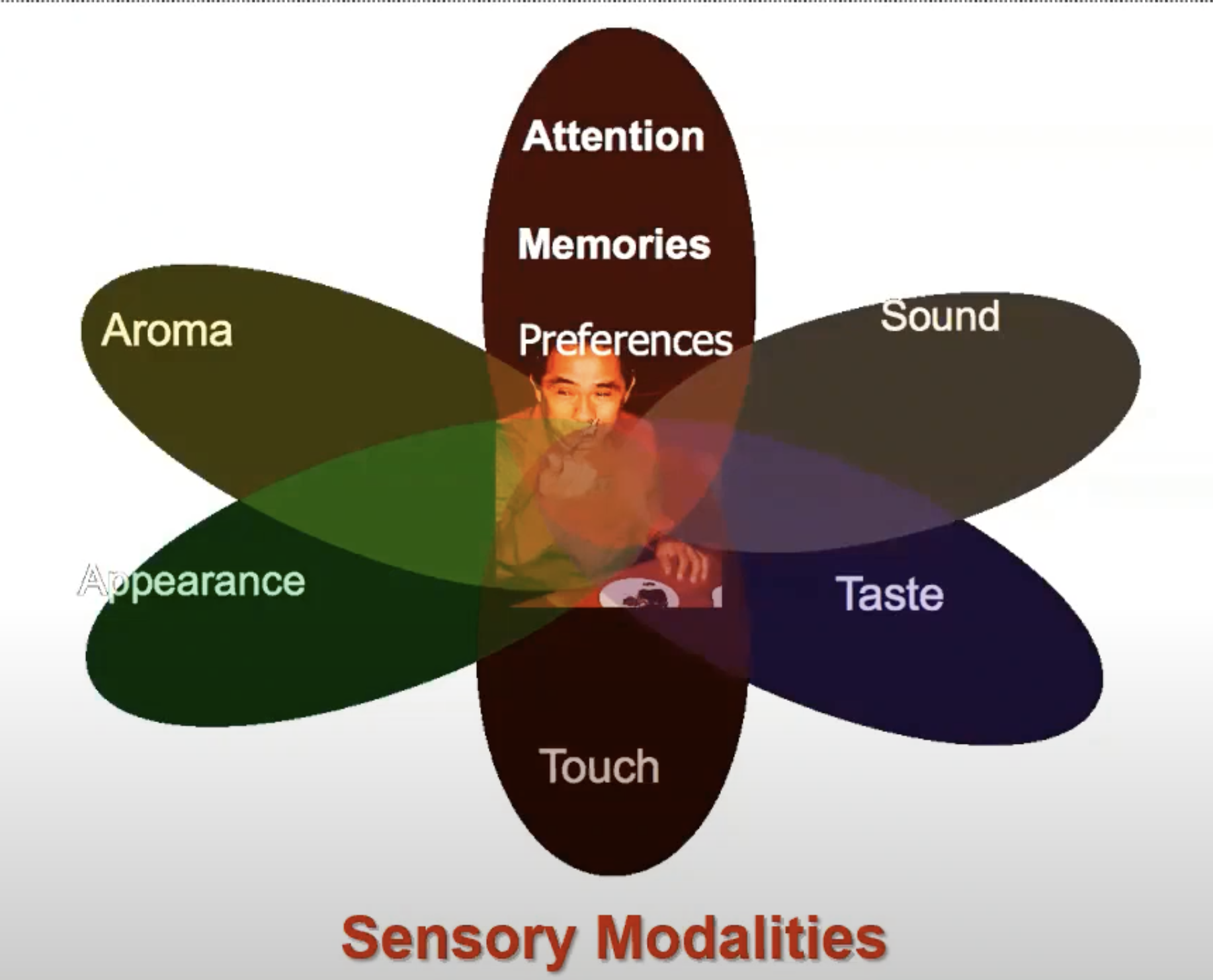
  • Here are the few most common modalities:
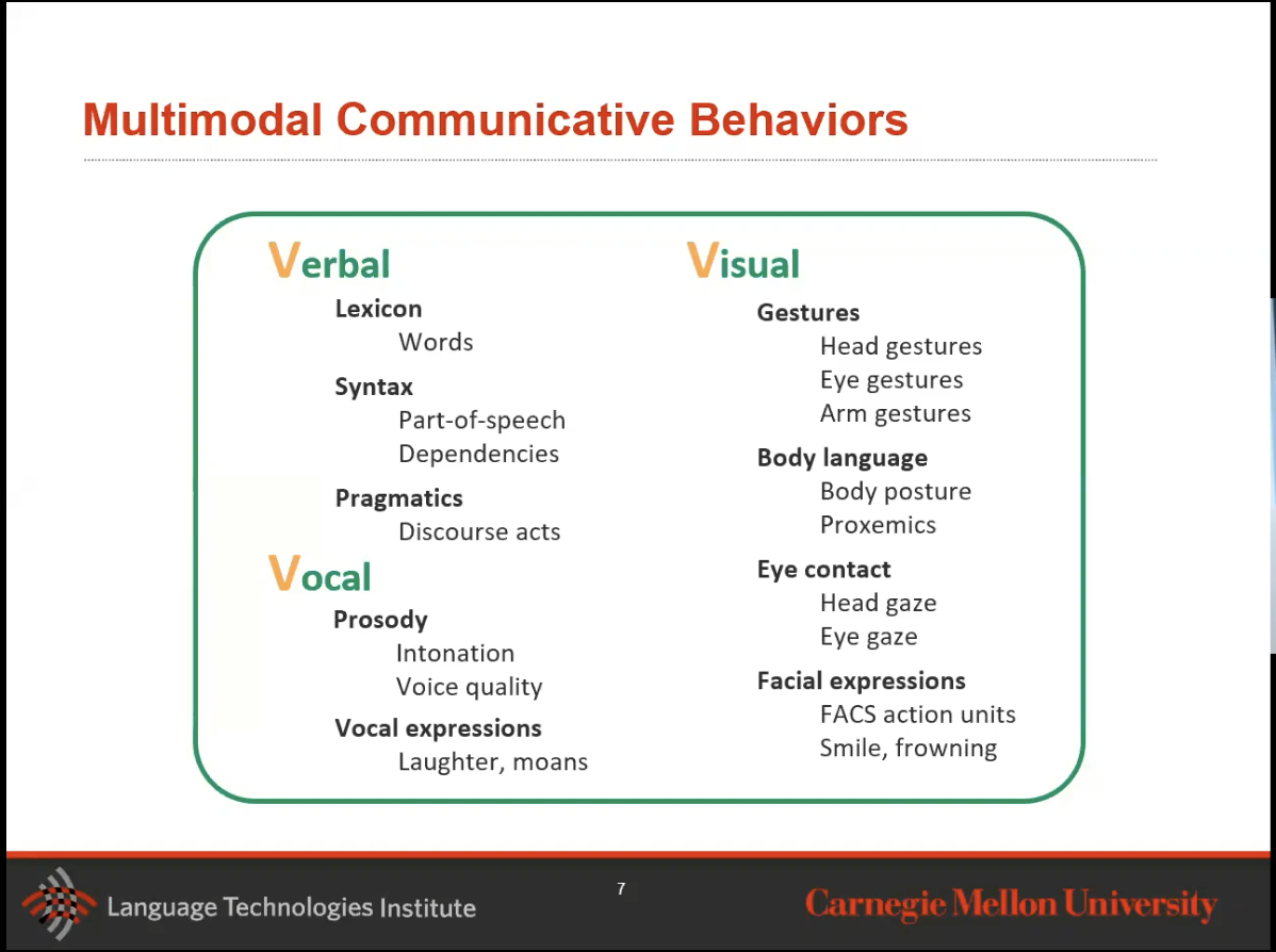
• In this course and notes, we will focus on language and vision as a few fundamental modalities.
• We will be talking about fusion, which is: to join information from two or more modalities to perform a prediction task. There are two types of fusion:
  • Early Fusion: Modalities are going to be concatenated early on.
  • Late Fusion: I need to do some processing in each modality early on before I combine them.
• We will delve into this and more as we go on.
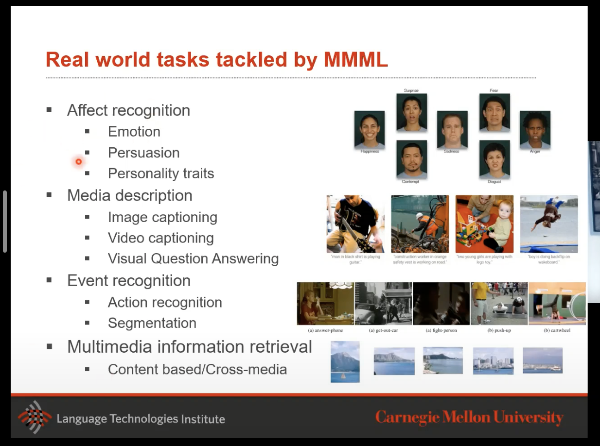
• Lastly, let’s look at a few real world examples into what MMML applications look like:

Unimodal Classification refresher

• Modal that only looks at one modality. Let’s take a step back and talk about this framework first.
• Let’s talk about a vision classification example, given an image, is it a dog or not?
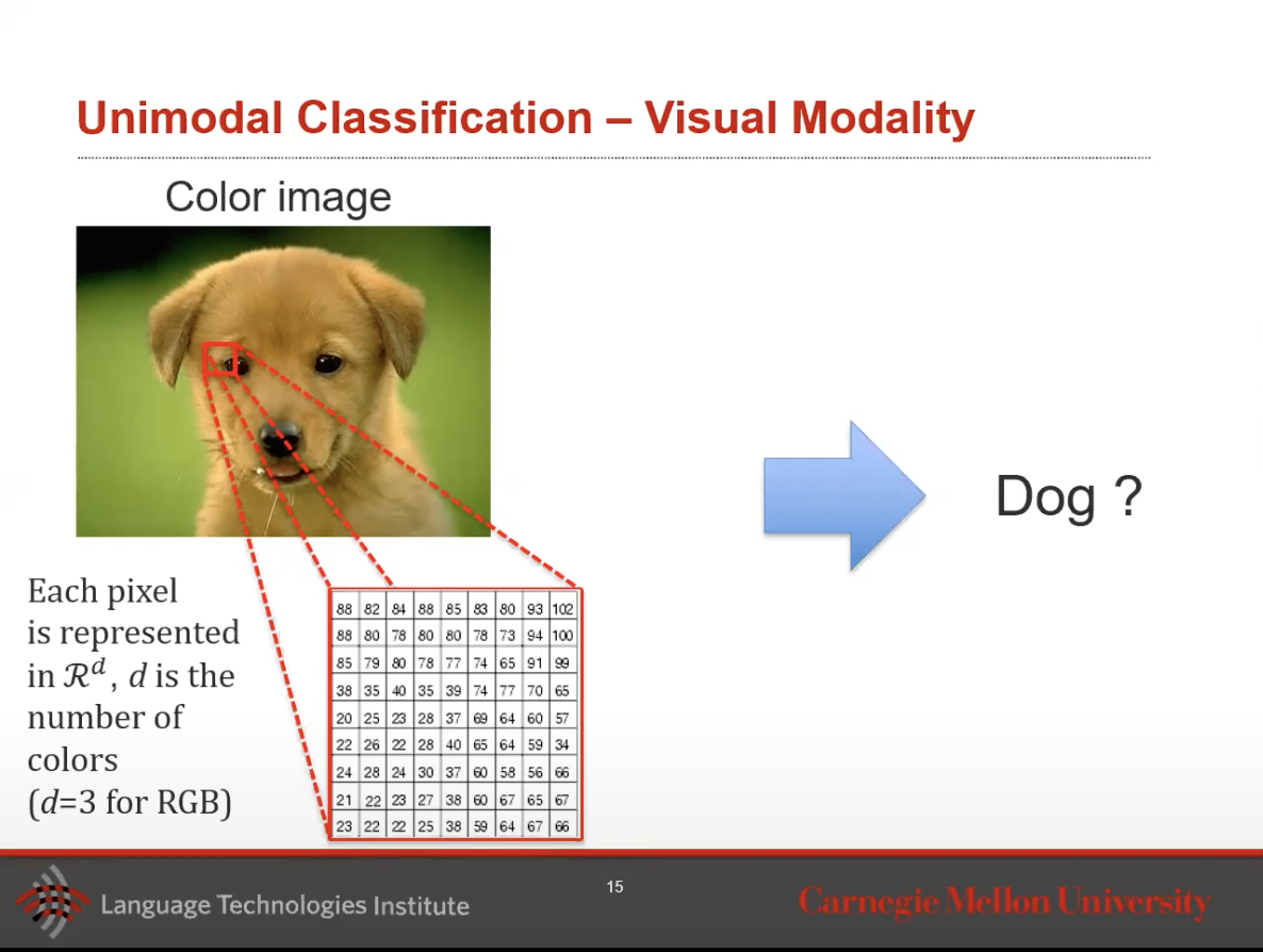
  • The \(x,y\) in the image above represent the position of the pixel. Note: if its a grayscale image, it’s a 2d matrix, otherwise its usually a 3d matrix where \(z\) would be color.
    • Its 3, 2d matrices stacked together for color images.
    • How do we solve our image classification problem here as most neural networks or classifiers except 2d matrices.
    • What you do to make this input vector is you take apart this 3d vector and you stack it upon each other like what’s show in the image below.
    • Then you will be able to get your object classification with a multi-class classification output.
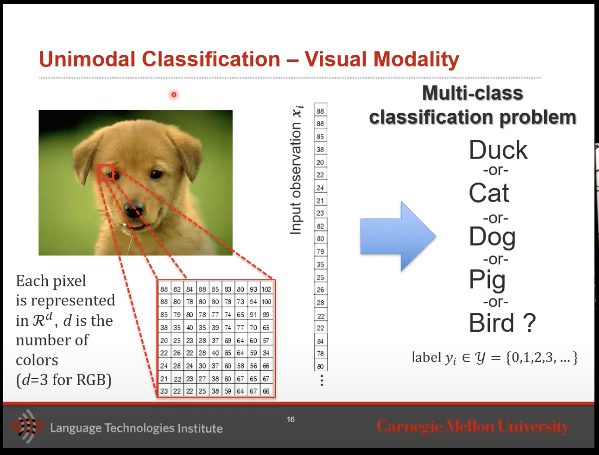
  • So for our unimodal models, we start with an input \(x\) which could just be a 3d matrix like above, run it through our trained model, and get a classification (single or multi-class) or regression output.
• Let’s now talk about a language (word, sentence, or paragraph) modality example.
  • Note: there are two types of language modality: written (text) and spoken (transcribed).
  • Let’s talk about a sentiment classification problem. Let’s say we have one word taken from a text and we want to understand if this is a positive or negative sentiment.
  • How would we do this?
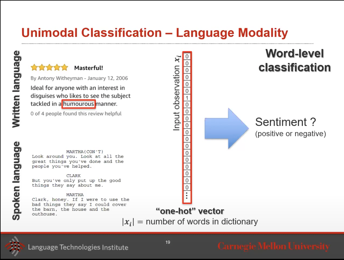
    • We will use a one-hot vector! This is a very long vector, its length is the length of the dictionary. This dictionary is what our model has created from the training set, counting all the unique words it has found.
    • For each of these words, we have one index entry in our vector.
    • Note: there are caveats here. Some people say if a word does not appear more than 10 times, we will not include it in the dictionary. Additionally, sometimes people use another corpus or an external example all together to generate their dictionary instead of making it part of their current classification task.
    • So this one-hot vector will serve as the input vector to our maximum entropy model (we will talk about this later) and we can either do sentiment classification or named-entity classification (names vs places vs entity) or part-of-speech tagging (verb, nound, adjective).
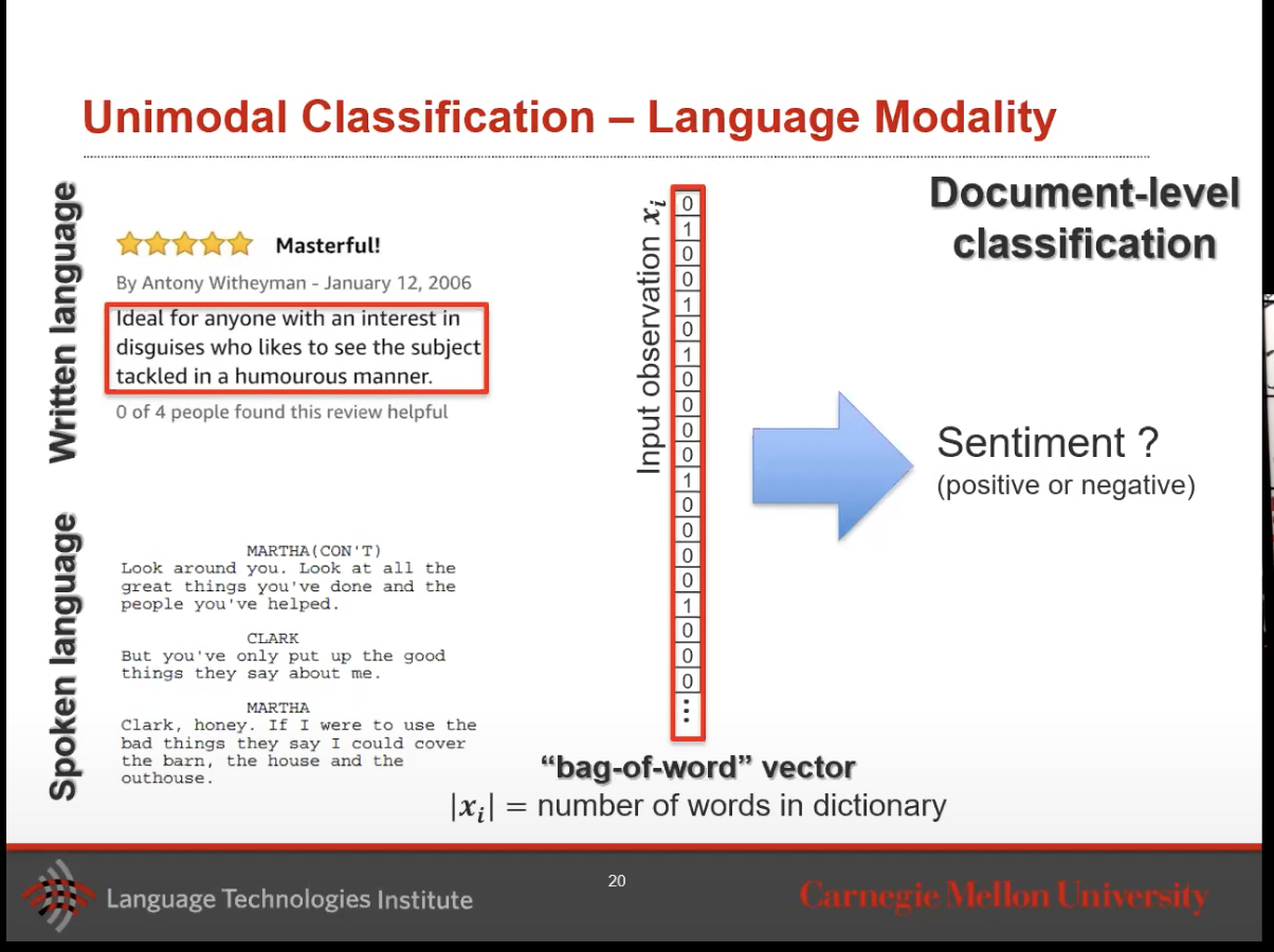
  • This is if we want to go granular and run our model on a word-by-word basis. However, what if we wanted to work with a larger quantity of text, say a sentence or a paragraph?
    • Now your input vector will become a bag-of-word vector. Its still a one-hot encoding because you have the same long dictionary, now you encode every word in that document, 1 if you see it, 0 otherwise.
    • You can then run the same tasks and do a sentiment classification as we did above.
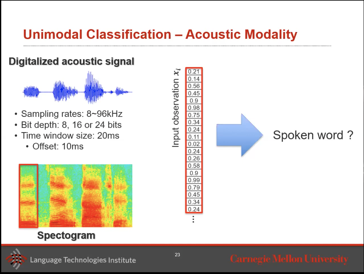
• Lastly, lets talk about acoustic modality.
  • Say you’re listening to someone, and you have an audio. Audio in its basics,is a very long 1D vector.
  • So you can use this vector and run a classification problem to transcribe the speech.
  • How is this done?
    • In practice, people slice the time windows in the audio signal and start processing on that dataset to create a Spectogram.
    • In this audio, we check how much low vs high frequency we get. That is what is recorded in a Spectogram in kilohertz.
    • We then take this Spectogram and convert it to an input vector for our model.
    • Outside of just transcription, you can use this to get emotion classification or voice quality from these models.
• We will be using these three modalities moving forward to talk about multimodal models and this is what this course will focus on.

Terminology

• Let’s go over a bit of terminology here that we will see further on in these notes.
• Dataset: Collection of labeled samples \(D\) : {\(x_i, y_i\)}.
  • Training set: Learn classifier on this training set
  • Validation set: Select optimal hyper-parameters here by looking at L1 or L2 functions. Basically want to see which hyperparameters give us the best results.
  • Test set: Never touch this during training. It evaluates the classifier on this hold-out test set.
• Nearest Neighbor: Simplest, yet still one of the most affective classifier.
  • At training time, the time complexity is O(1) and in test time it will be O(N)
  • It uses distance metrics to be able to find the nearest neighbor.
    • It will use L1 (Manhattan) or L2 (Eucledian) distance.

Neural Network or Linear Classification refresher

• Note: One neuron is called a linear classifier (depending on the activation function).
• Let’s talk about the parts, and functions of each of these parts, in the neural network.
• 1) Define a (linear) score function
  • What should be the prediction score for each class labels?
  • For ex, for the image classification problem of is this a dog, cat, bird, pig?
  • We will have one neuron for duck, one neuron for cat, one neural for bird and one for pig.
  • A neuron with a linear activation function is the function in the image below:
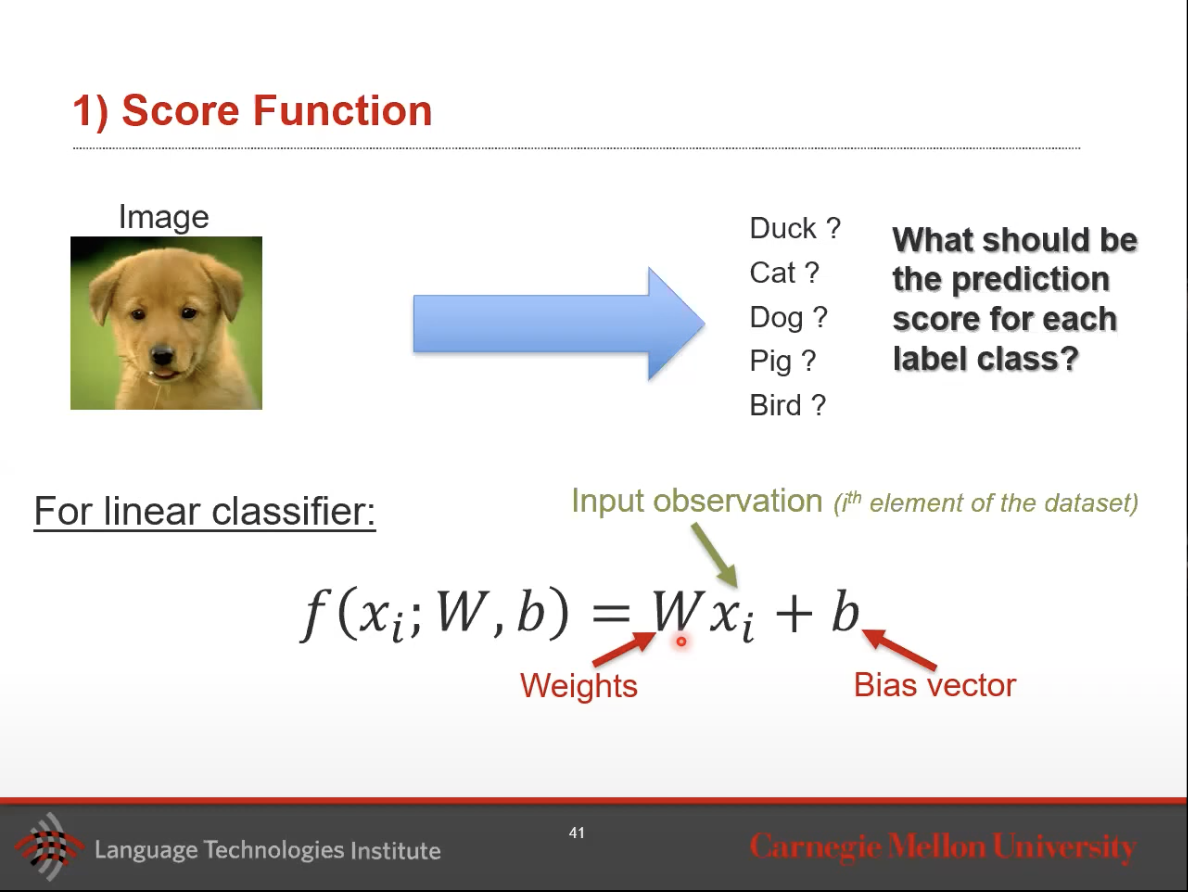
  • We want to learn the weights and biases here.
  • 2) Define the loss function (possibly non-linear)
  • 3) Optimize the weights of your parameters. (Think Gradient descent)
• Let’s also talk about multi-layer feed-forward neural networks.
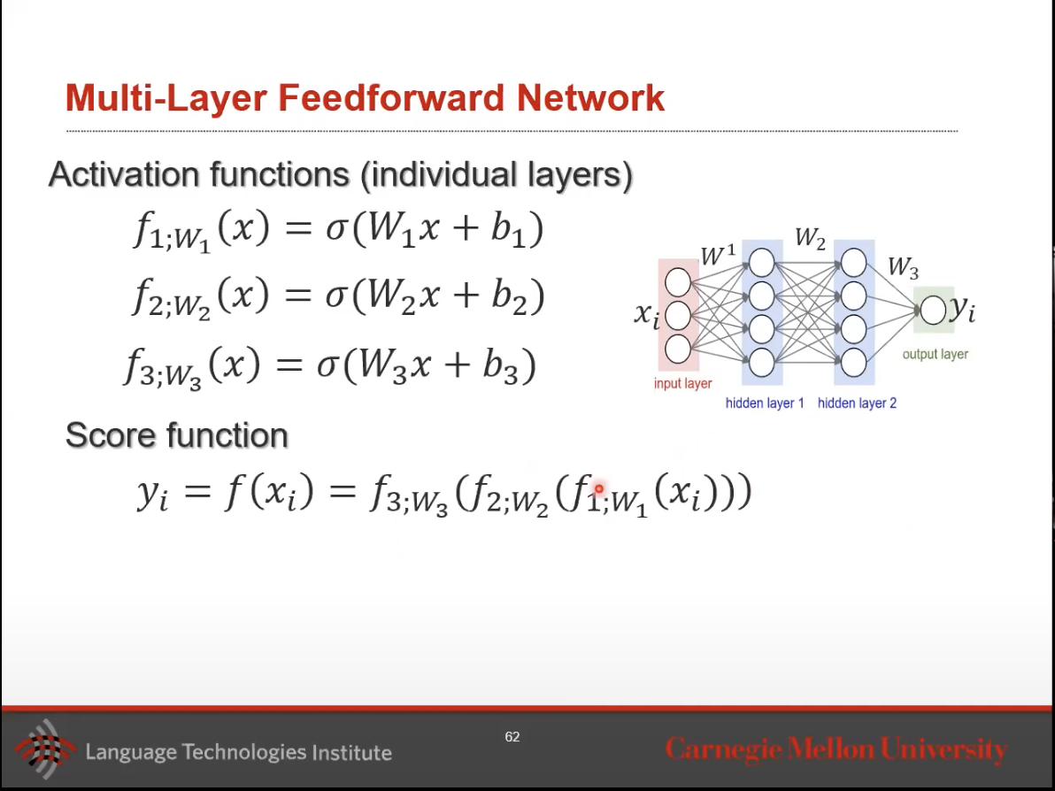
• As we can see, this multi-layer network is made up on an input layer, a few hidden layers, and then an output layer likely containing an activation function.
  • The output of each prior hidden layer serves as input to the layer that comes after it.
• Lastly, we want to end here by talking about just two more concepts:
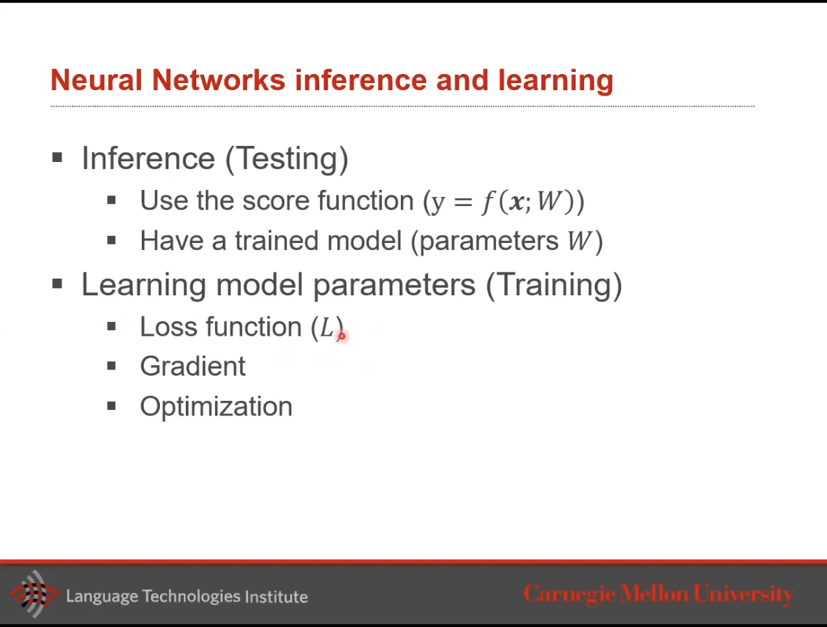
  • Inference: Used in testing. Inference can be thought of having input \(x\) and obtaining a score/output \(y\). It’s both the act of getting this score and using it.
  • Learning model parameter: Used at training time, you will run optimization using a gradient based approach.
    • Basically, we have our training data which is fixed. We want to learn the \(W\) weights and biases which leads to the minimum loss.