Internal Resource
- Overview
- ML Algorithms
- Fundamentals
- ML BREADTH QUESTIONS GENERIC
- REAL INTERVIEW EXAMPLE AND ADDITIONAL QUESTIONS
- General Questions Answers:
- 1. Linear Regression and Closed Form Solution
- 2. PCA and Bag of Words
- 3. Dropout and Ensemble Methods
- 4. Natural Gradient vs. Regular Gradient Descent
- 5. Avoiding Saddle Points
- 6. Tree Size in Random Forests vs. XGBoost
- 7. Neurons and Layers for 3D Data
- 8. Bayesian Optimization
- 9. Auto-Encoders vs. Variational Auto-Encoders
- 10. RBF Kernel and High Dimensions
- 11. Non-Convexity and Cross-Entropy Loss
- For Architects:
- NLP Answers:
- 1. Transformers vs RNNs
- 2. Encoder vs Decoder Transformers
- 3. Advantages of Encoder-Decoder Architecture
- 4. Word Embedding Methods and Evaluation
- 5. Projections of K,Q,V in Self-Attention
- 6. Generating Paragraphs from LLM Outputs
- 7. CNNs and Translation
- 8. Training LLMs for Low-Resource Languages
- 9. Fine-Tuning LLMs
- 10. Positional Encodings in Transformers
- 11. Output of Transformer Layers
- 12. Evaluating OCR Outputs
- 13. Rare Use of Untrained Transformers
- 14. Flexible vs Strict Conductive Bias
- 15. Learning Rates in Training LLMs
- 16. Larger Prompts in LLMs
- 17. Prefix vs Causal Language Models
- 18. Named Entity Recognition vs Linking
- 19. Automated Evaluation of LLM Output
- High-Bias vs. High-Variance Model:
- Identifying Overfitting in Deep Learning Model
- Architectural Strategies to Prevent Overfitting
- Data Strategies to Prevent Overfitting
- Augmentation Strategies in NLP and CV Domains
- CNN Structure
- DROPOUT
- BATCHNORM
- How do we deal with real-time data in recommender systems for batchnorm mean and variance calculation for normalization?
- 1. Moving Average During Training:
- 2. Periodic Model Updates:
- 3. Adaptive Normalization:
- 4. Layer Normalization:
- 5. Instance Normalization:
- 6. Batch Renormalization:
- 7. Feature Engineering:
- 8. Hybrid Approaches:
- Conclusion:
- If the averages go to zero during real time calculation of batchnorm statistics, how will you make sure that your computed batchnorm statistics make any sense
- 1. Check Data Preprocessing:
- 2. Monitor Learning Rate:
- 3. Analyze Model Initialization:
- 4. Regularize the Model:
- 5. Adjust BatchNorm Hyperparameters:
- 6. Use Stable Batch Sizes:
- 7. Evaluate Model Architecture:
- 8. Consider Alternative Normalization Techniques:
- 9. Logging and Alerting:
- 10. Use Running Averages in Inference:
- Conclusion:
- Differences between CNN and FCNN
- CNN Kernel Size Considerations
- Structure Comparison: CNNs vs. Language Models
- Self-Attention vs. Cross-Attention
- Multiple Heads in Self-Attention Layer
- ViT and Advantages in Vision Models
- Self-Supervised Learning
- Modern LLMs
- Generative AI
- Hallucinations
- Vector Database
- Agent in AI
- Diffusion Models
- SnapChat interview
- ChatGPT vs GPT3
- Generating music with text or images
- Stable Diffusion
- ML Youtube channels
- DALLE-2
- Forward-Forward Algorithm
- ChatGPT
- ML for Ads Ranking RecSys
- Is PageRank still used at Google
- CLIP
- Quick Feature Selection Method
- Overfitting
- Pruning
- Information Retrieval Metrics
- XGBoost
- Data Parallelization by Sebastian Raschka
- Top 5 basic checks when trianing deep learning models
- A list of 5 techniques to optimize deep neural network model performance during inference
- Links for MLOPS
- Architecture
- Recommender Engine
- How to detect Data Drift
- Prevent data drift
- Explain reasoning behind offline and online gap in ML system evaluation and mitigation strategies?
- How do wide and deep models handle feature crossing in recommender systems?
- How to decompose Bias and Variance from the Data
- Feature Selection Method
- For typical recommendation system, a common practice is to continuously train the model. Suppose that we launched a 6 model ago and we have continuously trained it. Consider that if we trained a month starting off with the 6 month ago checkpoint and trained with 3 months of fresh data. How do we use the production model to make the new model with 3 months of data better?
- How are ID features handled in LLM recommender models?
- Self Instruct aligning language models with self generated instructions
- How do you handle hashing for a large billion-scale ID cardinality?
- What kind of feature crossing techniques in recommender systems?
- ANN and it’s selection criteria
- How do we handle categorical features in recommender systems?
- Is there any downside to Feature Hashing (Hashing Trick)?
- How do wide and deep models handle feature crossing in recommender systems ?
- Deep and Cross
- What does feature crossing mean? how do you handle high cardinality in data when crossing?
- For a recommender system’s training data, say we have 100M data samples, 5000 for retrieval, 5 for ranking. For the ranking stage, we want to log features. How best do we log for features since the ones that didn’t get to ranking could also be relevant?
- How do we compress features being stored for retrieval and ranking given space would be an issue?
- Tell me Deep and Cross vs Deep and Wide and draw the architecture in ascii, comparative analysis and focus on sparse,dense features and feature crossing
- Train Validation Test split
- Why you cant tune Hyperparameters on train
- L1 vs L2
- To Answer
Overview
- The content below is a work in progress and is a collection of content from Damien Benveniste’s linkedIn posts that can be found here and Prithivi Da.
- Content is also from Sebastian Raschka
ML Algorithms
Fundamentals
Thank you for providing a comprehensive list of Machine Learning questions along with some answers. Below are extended answers and discussions on some of the questions you presented. Given the breadth of the topics, I’ll address a subset of questions for more thorough answers.
ML BREADTH QUESTIONS GENERIC
Q: How might you build a classifier when you only have a small amount of labelled data, and just getting more data isn’t an option? A: Additional approaches might also include utilizing few-shot learning, where the model is designed to gain understanding with very minimal data by leveraging prior knowledge learned from related tasks. One-shot learning and zero-shot learning strategies can also be considered, which involve learning from one or zero examples respectively, often by leveraging semantic relationships between classes.
Q: I want to test the effectiveness of a change to my web service in a way which is statistically sound. How can I do this? A: It’s crucial to ensure that the participants in each group (treatment and control) are randomized effectively to avoid biases and to ensure that the results are generalizable. It’s also essential to determine the sample size needed to detect a statistically significant difference (if it exists) prior to conducting the test, to avoid type II errors. Additionally, considering factors like seasonality, which might impact the user behavior during the test period, is pivotal.
Q: I want to learn from textual data. How do I map text to a numerical form appropriate for classification or annotation or translation? A: Beyond bag of words and TF-IDF, leveraging word embeddings like Word2Vec, GloVe, or even more advanced transformer-based approaches like BERT embeddings can be very effective in capturing semantic meanings of words and can be pivotal for tasks like translation. Embedding layers can also be learned in an end-to-end fashion during model training for specific tasks.
Q: I want to recommend a set of items to a customer. What makes this different from other learning tasks? A: This problem involves user-user and item-item interactions, which make it necessary to understand both the properties of items and the preferences of users. Cold start problems (where a new user or item has no interaction history) are also a unique challenge in recommendation systems. Hybrid recommendation systems that utilize content-based and collaborative filtering methods could provide more robust recommendations and alleviate some cold start issues.
Q: If I receive input, output pairs continuously from a stream, with no guarantee that the mapping is constant in time (i.e. non-stationary distribution), what can I do? How can I learn a good model? A: Implementing a concept drift detection mechanism will be critical in this situation to detect when the statistical properties of the model inputs are changing. Once detected, the model could be incrementally updated using online learning approaches or periodically retrained with newer data to adapt to the changing distributions.
REAL INTERVIEW EXAMPLE AND ADDITIONAL QUESTIONS
Q: What is unsupervised learning? A: Unsupervised learning involves modeling with datasets that contain only input data and no corresponding output labels. The system tries to learn the patterns and the structure from the data without any labeled responses. Common approaches include clustering and association algorithms.
Q: What is the bias-variance trade-off? A: The bias-variance trade-off is a fundamental concept in the field of machine learning that relates to the error of a model. High bias indicates a model that is too simple, leading to underfitting, while high variance indicates a model that is too complex, leading to overfitting. The trade-off entails finding a balance where increasing bias will decrease variance and vice-versa, and finding the optimal model complexity to minimize the total error.
Q: How can you quantify the uncertainty in your prediction? A: Quantifying uncertainty can involve techniques such as Bayesian methods that allow the model to express uncertainty about its parameters and predictions. Alternatively, bootstrapping methods can generate empirical confidence intervals for predictions, allowing a range of likely values to be expressed.
Q: Under which conditions does SGD converge to the global optimum? A: For convex loss surfaces, SGD will converge to a global optimum given an appropriately decreasing learning rate. For non-convex surfaces, such as those encountered while training deep neural networks, SGD may find different local minima or saddle points depending on the initialization and stochasticity of the descent path.
These answers provide a starting point and could be expanded upon in a dialogue during an interview to showcase understanding, experience, and problem-solving ability in these areas. If you’d like more detail on a particular question, please let me know!
General Questions Answers:
1. Linear Regression and Closed Form Solution
Linear regression supports a closed form solution when the matrix $(X^TX)$ is non-singular, i.e., it is invertible. The closed-form solution is given by $\beta = (X^TX)^{-1}X^Ty$ and is computationally efficient compared to iterative methods, especially for small datasets.
2. PCA and Bag of Words
- PCA (Principal Component Analysis): PCA is a dimensionality reduction technique that finds the axes (principal components) in the feature space along which the data varies the most. It’s useful in reducing computational complexity, mitigating the curse of dimensionality, and visualizing high-dimensional data.
-
With Bag of Words: PCA can be used with Bag of Words representation to reduce dimensionality, but care is needed as BoW is sparse and high-dimensional, so applying PCA directly may not preserve interpretability.
Follow-up: The covariance matrix in PCA is used because it captures the variance and linear correlation between different features. Eigenvectors of the covariance matrix indicate the directions of maximum variance (principal components).
What is the diff between spearman/pearson correlation coefficienct?
- The main differences between Spearman’s and Pearson’s correlation coefficients are:
- Type of data used:
- Spearman’s correlation uses ranked/ordinal data, while Pearson’s uses continuous/interval data. Spearman’s works on data that is converted to ranks.
- Type of relationship measured:
- Spearman’s measures the monotonic relationship between two variables, while Pearson’s measures the linear relationship. Spearman’s will detect any monotonic association whereas Pearson’s only detects linear associations.
- Sensitivity to outliers:
- Spearman’s correlation is less sensitive to outliers compared to Pearson’s. Since Spearman’s uses ranked data, outliers have less impact. Pearson’s can be significantly affected by outliers.
- Range of values:
- Spearman’s correlation coefficient ranges from -1 to +1. Pearson’s ranges from -1 to 1 but can only be +1 or -1 if the relationship is perfectly linear.
- Statistical assumptions:
- Spearman’s makes fewer assumptions about the distribution of data. Pearson’s assumes the data is normally distributed and a linear relationship exists between the variables.
- Use cases:
- Spearman’s is used when data is ordinal, ranked, or does not follow a normal distribution. Pearson’s is appropriate for interval/ratio data that is normally distributed and where a linear relationship is expected.
- In summary, Spearman’s assesses monotonic relationships, is more robust to outliers, and makes fewer distributional assumptions, while Pearson’s assesses linear relationships but is more sensitive to non-normal data and outliers.
3. Dropout and Ensemble Methods
Dropout, which involves randomly deactivating certain neurons during training, can be likened to ensemble methods as it prevents neurons from becoming too specialized, enforcing a form of model averaging. During inference, all neurons are used, and their outputs are averaged, similar to an ensemble of different networks.
4. Natural Gradient vs. Regular Gradient Descent
Using the natural gradient (which considers the curvature of the loss surface) can be computationally expensive and memory-intensive because it involves computing and inverting the Fisher information matrix, making it less practical for large-scale applications compared to first-order methods like gradient descent.
5. Avoiding Saddle Points
Methods to avoid saddle points include using optimization algorithms like SGD with momentum (which can traverse saddle points by utilizing past gradients) or adopting second-order optimization methods, such as Newton’s method, which can navigate through saddle points more efficiently.
6. Tree Size in Random Forests vs. XGBoost
- Random Forests: Large trees are employed to capture complex patterns and reduce bias, with the averaging of numerous trees mitigating overfitting.
- XGBoost: Smaller trees (weak learners) are utilized to maintain model simplicity, prevent overfitting, and allow subsequent trees to correct previous ones’ errors, focusing on areas where performance can be improved.
7. Neurons and Layers for 3D Data
The minimum number of neurons and layers for a 3-feature NN could technically be very small (even a single-layer perceptron) for simple tasks. However, the ideal architecture depends heavily on the complexity of the mapping from input to output, and it often requires experimental tuning to determine an effective network size.
8. Bayesian Optimization
- When to Use: Bayesian optimization is especially useful for optimizing expensive or noisy objective functions.
- How it Works: It models the objective function using a probabilistic model (like Gaussian Process) and uses an acquisition function to decide where to sample next, balancing exploration and exploitation.
9. Auto-Encoders vs. Variational Auto-Encoders
- Auto-Encoders: Aim to reproduce the input by learning an encoding and decoding process.
- VAEs: VAEs also learn to generate new data by introducing a probabilistic aspect. The loss function of VAE includes a reconstruction term and a regularization term, which enforces the learned encodings to follow a specified probability distribution, typically a Gaussian.
10. RBF Kernel and High Dimensions
-
Dimensions: The Radial Basis Function (RBF) kernel implicitly projects data into an infinite-dimensional space.
Follow-up1: Using the kernel trick, we compute dot products in this high-dimensional space without explicitly performing the projection, preventing a computational blowup.
Follow-up2: Despite the projection to high-dimensional spaces, overfitting is mitigated as the complexity of the decision function is regulated by the margin, which is inversely related to the norm of the weight vector in the feature space.
11. Non-Convexity and Cross-Entropy Loss
The empirical success of optimizing non-convex loss functions, like cross-entropy in deep learning, might be attributed to the properties of high-dimensional optimization landscapes and the robustness of stochastic gradient descent (SGD) in navigating them, often finding broad, nearly-global minima that generalize well.
For Architects:
1. LORA
LORA (Layer-wise Optimization of Representations and Attention) involves optimizing large-scale models like GPT using layer-wise adaptive learning rates, which help in refining important layers and capturing more fine-grained patterns during fine-tuning.
2.-4. Web Scraping, Data Cleaning, and Deduplication
- For web scraping, ensure compliance with legal and ethical guidelines, use robust scrapers like Beautiful Soup or Scrapy, and consider challenges like CAPTCHAs or dynamic content.
- Cleaning might involve handling missing data, correcting inconsistencies, or managing noisy labels.
- For deduplication, hashing techniques or locality-sensitive hashing could be utilized to identify similar pages without computing pairwise distances exhaustively.
5. Batch Sizes in LLM Training
Batch sizes would depend on factors like the memory constraints of the hardware, the stability of training, and convergence properties. Larger batches provide more accurate gradient estimates but are computationally expensive.
6. Machines for Inference
Typically, GPUs or specialized ASICs (like Google’s TPUs) are employed for inference due to their parallelization capabilities and efficient handling of matrix operations.
7. FPGAs for Inference
FPGAs can indeed be used for inference, offering advantages like reconfigurability, potential for low-latency operations, and power efficiency. They can be tailored to specific applications, ensuring efficient utilization of resources.
8. Complexity of Training Transformers
The complexity of training transformers is $O(n^2 \cdot d)$ for a sequence of length $n$ and embedding dimension $d$, primarily due to the self-attention mechanism, making long sequences computationally expensive to process.
9. Avoiding Vanishing Gradient in Transformers
Transformers utilize layer normalization and residual connections to mitigate the vanishing gradient problem, ensuring that gradients can flow through the network during backpropagation, even across many layers.
NLP Answers:
1. Transformers vs RNNs
Transformers tend to outperform RNNs mainly because they allow parallel processing of sequences and can capture dependencies regardless of distance between elements in a sequence, thanks to the self-attention mechanism. This alleviates the long-term dependency issues often encountered with RNNs and enables Transformers to handle longer contexts more effectively.
2. Encoder vs Decoder Transformers
An encoder transformer processes input sequences and compresses this information into context representations. A decoder transformer generates output sequences, often utilizing context from an encoder. Encoders handle input data, while decoders generate output data, sometimes conditioned on encoder representations.
3. Advantages of Encoder-Decoder Architecture
Using an encoder-decoder architecture allows for handling variable-length input and output sequences, facilitates learning from a context created by the encoder, and permits the model to generalize across different domains by separating the representation learning and generation processes.
4. Word Embedding Methods and Evaluation
- Methods: Word2Vec, GloVe, and FastText.
- Evaluation: Intrinsic evaluation using tasks like analogy solving or similarity computations and extrinsic evaluation by integrating embeddings into downstream tasks like classification and observing performance.
5. Projections of K,Q,V in Self-Attention
Using projections (linear transformations) of Key (K), Query (Q), and Value (V) in self-attention allows the model to learn optimal representations and introduces learnable parameters that enable the model to focus on different aspects of the input sequence.
6. Generating Paragraphs from LLM Outputs
Generated paragraphs are formed by sampling tokens from the probability distributions outputted by the LLM, typically using methods like greedy decoding, beam search, or nucleus sampling, and concatenating these tokens to form coherent text.
7. CNNs and Translation
CNNs have fallen out of favor for translation as Transformers offer advantages like handling variable-length sequences and capturing long-term dependencies more efficiently due to the self-attention mechanism.
8. Training LLMs for Low-Resource Languages
For low-resource languages, one might leverage transfer learning from high-resource languages, utilize data augmentation techniques, or employ semi-supervised learning approaches to maximize the utility of available data.
9. Fine-Tuning LLMs
Fine-tuning can be done using techniques like elastic weight consolidation or knowledge distillation to preserve previously learned knowledge while adapting to new tasks.
10. Positional Encodings in Transformers
Positional encodings are used in Transformers because, unlike RNNs, they do not have an inherent sense of order or position, thus requiring explicit positional information to understand sequence order.
11. Output of Transformer Layers
Each transformer layer outputs a set of representations for the input tokens, wherein each representation is influenced by all other tokens in the input due to self-attention.
12. Evaluating OCR Outputs
Evaluation might involve using character-level metrics like Character Error Rate (CER) or utilizing application-specific metrics if no ground truth is available, and employing unsupervised or semi-supervised methods to derive insights.
13. Rare Use of Untrained Transformers
Using pre-trained Transformers is prevalent as training them from scratch requires enormous computational resources, and pre-training provides a strong initialization that aids in various downstream tasks.
14. Flexible vs Strict Conductive Bias
A more flexible conductive bias might be better when exploring varied solutions and novel tasks, while a stricter bias could be beneficial in ensuring adherence to known good practices or ethical guidelines.
15. Learning Rates in Training LLMs
Gradually increasing learning rates (learning rate scheduling) helps in avoiding local minima initially and then fine-tuning the model in later stages for better convergence.
16. Larger Prompts in LLMs
Larger prompts tend to provide more context and clearer instructions to LLMs, facilitating the generation of more relevant and coherent responses.
17. Prefix vs Causal Language Models
Prefix language models condition on both past and future tokens during training, whereas causal language models (like GPT) only condition on preceding tokens, generating sequences in a left-to-right manner.
18. Named Entity Recognition vs Linking
- NER: Identifies entities in text and classifies them into predefined categories.
- NEL (Entity Linking): Goes a step further to link identified entities to entities in a knowledge base. Applications might include information extraction, knowledge graph construction, and question answering.
19. Automated Evaluation of LLM Output
Automated evaluation could involve using metrics like BLEU, ROUGE, or METEOR for comparing generated text against reference text, or employing task-specific evaluation metrics to assess performance on intended applications.
Feel free to dive deeper into any topic or ask for further clarifications!
High-Bias vs. High-Variance Model:
- High-Bias Model:
- Tends to oversimplify the model, not capturing the underlying patterns in the data.
- Relates to underfitting because the model cannot perform well due to its simplistic assumptions and inability to learn the data’s intrinsic structure.
- High-Variance Model:
- Overcomplicates the model, capturing too much of the data’s noise along with the underlying patterns.
- Relates to overfitting as the model is too sensitive and tailors itself too closely to the training data, capturing noise as if it were a real pattern.
Identifying Overfitting in Deep Learning Model
- Divergence of Metrics: When the training loss continues to decrease, but validation loss starts increasing, it’s a clear sign of overfitting.
- Visualization: Plotting learning curves for training and validation can visually reveal overfitting as the curves will start to diverge.
- Performance Metrics: A model that performs exceptionally well on training data but poorly on validation/test data is likely overfitting.
Architectural Strategies to Prevent Overfitting
- Regularization (L1/L2): Adds a penalty term to the loss function, discouraging overly complex models by penalizing large weights.
- Dropout: Randomly sets a fraction of the input units to 0 at each update during training, helping to prevent unit co-adaptation.
- Early Stopping: Ends training once the model’s performance ceases to improve on a held-out validation dataset.
- Decreasing Representational Capacity: Reducing the size or complexity of the model (like the number of parameters or layers) to make it harder for it to memorize the training data.
Data Strategies to Prevent Overfitting
- More Data: Providing more examples can reduce overfitting as it gives more information for the model to learn generalized patterns.
- Data Augmentation/Noise Injection: Introduces variability and helps the model generalize better to unseen data.
- Cross-Validation: Ensures robust evaluation and can help in tuning the model without exploiting test data.
- Feature Engineering: Involves choosing the most relevant features to train on, which could reduce complexity and overfitting.
Augmentation Strategies in NLP and CV Domains
- CV Domain:
- Rotate/Crop: Altering the orientation or cropping images to create variations.
- Jitter: Adding small random perturbations to pixel values to introduce noise.
- NLP Domain:
- Backtranslation: Translating text to another language and then back to the original to create a slightly different version.
- Generative Augmentation: Using language models to generate new sentences or text snippets that convey similar meanings.
CNN Structure
Answer: Convolutional Neural Networks (CNNs) consist of an input layer, multiple hidden layers, and an output layer. Hidden layers often include convolutional layers, pooling layers, and fully connected layers. Convolutional layers apply filters to the input to create feature maps. Activation functions like ReLU, Sigmoid, or Tanh introduce non-linearity and are applied post-convolution. Pooling layers reduce spatial dimensions (width & height) to reduce the parameter count and therefore computation in the network. Dropouts can be applied to prevent overfitting by randomly setting a fraction of input units to 0 at each update during training time. Batch normalization helps to make the network stable and converge faster by normalizing the inputs in the intermediate layers.
DROPOUT
Answer: Dropout is a regularization technique used to prevent overfitting in neural networks. During training, a percentage (p%) of the neurons in the layer where dropout is applied are randomly set to zero, thereby dropping out random features/interactions. At inference time, all neurons are used but their outputs are scaled down by the dropout rate to balance the larger number of active neurons during testing compared to training.
BATCHNORM
Answer: Batch Normalization (BatchNorm) is a technique to automatically scale the inputs to a neural network layer, ensuring that the activations do not reach extremely high or low values. It works by normalizing the mini-batch data (subtracting batch mean and dividing by batch standard deviation), which can accelerate the training process and make it less sensitive to the initial weights. The operation also involves learning two parameters, scale and shift, to allow the model to undo the normalization if it finds it beneficial.
How do we deal with real-time data in recommender systems for batchnorm mean and variance calculation for normalization?
-
Here are some strategies to handle real-time data in recommender systems when using batch normalization:
-
Moving averages - Keep running averages of means and variances as new data comes in. Use these moving averages for normalization statistics rather than batch statistics.
-
Mini-batch updates - Periodically update normalization stats by passing mini-batches of new data through the model. Keeps the stats up-to-date.
-
Separate streaming normalization - Use a separate normalization layer tuned on streaming data before the main model.
-
Feature-wise normalization - Compute means and variances for each feature separately offline. Apply per-feature normalization.
-
Hybrid offline and streaming stats - Initialize with offline dataset statistics, then continuously update with streaming data.
-
Maintain stream statistics - Explicitly compute streaming counts, means, variances over time windows for normalization.
-
Decaying averages - Slowly decay and update averaging weights to give more priority to recent data.
-
Predictive normalization - Use model like RNNs to predict expected normalization parameters for new data.
- Model finetuning - Adaptively finetune model on new data periodically to adjust for shifts in data.
- The core idea is to continuously update the batch normalization statistics on the fly as new data arrives rather than using static offline datasets. This allows the model to adapt to real-time data streams.
- Handling real-time data in recommender systems, particularly in the context of using Batch Normalization (BatchNorm), requires careful consideration. BatchNorm, as typically implemented, relies on batch statistics (mean and variance) calculated during training. In a real-time setting, the data distribution can shift, making these precomputed statistics less representative. Here are several strategies to address this challenge:
1. Moving Average During Training:
- Description: Use a moving average of mean and variance during training instead of batch-wise statistics. This approach can provide a more general representation of the dataset.
- Application: During inference or real-time recommendations, these moving averages are used instead of batch-specific statistics.
2. Periodic Model Updates:
- Description: Regularly update the model with new data to ensure the batch statistics are representative of the current data distribution.
- Application: Implement a system where the model is retrained or fine-tuned periodically (e.g., daily, weekly) with the latest data.
3. Adaptive Normalization:
- Description: Adapt the normalization statistics based on incoming real-time data. This could involve a gradual update of the mean and variance estimates.
- Application: Design a system where the normalization statistics are updated in a rolling manner as new data comes in, though care must be taken to avoid drastic changes based on anomalous data.
4. Layer Normalization:
- Description: Consider using Layer Normalization instead of BatchNorm. Layer Normalization normalizes across features instead of the batch dimension, making it less sensitive to batch size and composition.
- Application: Useful in scenarios where batch sizes are small or vary significantly, which is often the case in real-time systems.
5. Instance Normalization:
- Description: Similar to Layer Normalization, Instance Normalization normalizes each individual data point independently.
- Application: This can be particularly effective for personalized recommender systems, where the focus is on individual user-item interactions.
6. Batch Renormalization:
- Description: Batch Renormalization (introduced by Sergey Ioffe in 2017) modifies BatchNorm to use a blend of batch statistics and moving averages. This can help in scenarios where the batch size is small or the data distribution changes over time.
- Application: Particularly useful in online learning scenarios where data is continuously updating.
7. Feature Engineering:
- Description: Focus on robust feature engineering that reduces the dependency on normalization techniques.
- Application: Use features that are inherently stable and less prone to shifts in distribution.
8. Hybrid Approaches:
- Description: Combine real-time updates with periodic retraining. Use real-time data to adjust the model slightly while relying on periodic comprehensive updates.
- Application: Balances the need for up-to-date recommendations with the stability of a periodically trained model.
Conclusion:
Each of these approaches has its own trade-offs and applicability depending on the specific requirements and constraints of the recommender system. In practice, a combination of these strategies might be employed to effectively handle real-time data while maintaining the benefits of Batch Normalization. The key is to ensure that the system remains adaptive and responsive to the changing data landscape without compromising the stability and accuracy of the recommendations.
If the averages go to zero during real time calculation of batchnorm statistics, how will you make sure that your computed batchnorm statistics make any sense
- If the averages (means) and variances computed for Batch Normalization (BatchNorm) approach zero during real-time calculation, it could indicate a few issues with the data or the model, such as vanishing gradients, improper data preprocessing, or model architecture issues. Ensuring that BatchNorm statistics are meaningful and effective, especially in a real-time setting, requires addressing these potential issues:
1. Check Data Preprocessing:
- Ensure that the input data is preprocessed correctly. Improper scaling or normalization of inputs can lead to degenerate BatchNorm statistics.
- Verify that there are no issues with the data pipeline, such as incorrectly applied transformations or data corruption.
2. Monitor Learning Rate:
- A high learning rate can cause the model parameters, including BatchNorm parameters, to change too rapidly, potentially leading to vanishing or exploding gradients.
- Try reducing the learning rate to see if it stabilizes the BatchNorm statistics.
3. Analyze Model Initialization:
- Inspect the initialization of the model weights. Poor initialization can lead to vanishing or exploding gradients, which in turn affect BatchNorm statistics.
- Consider using initialization methods like Xavier or He initialization, which are designed to maintain the scale of the gradients.
4. Regularize the Model:
- Implement regularization techniques like dropout, L1/L2 regularization, or use techniques like gradient clipping to prevent the model from diverging.
5. Adjust BatchNorm Hyperparameters:
- Experiment with different values for the momentum parameter in BatchNorm. A lower momentum value places more weight on the current batch statistics.
- Check the epsilon value used in BatchNorm to avoid division by zero.
6. Use Stable Batch Sizes:
- In real-time systems, ensure that the batch size is consistent and sufficiently large. Small batch sizes can lead to unstable BatchNorm statistics due to insufficient data points.
7. Evaluate Model Architecture:
- Sometimes the issue might lie in the model architecture. For example, too deep a network can lead to vanishing gradients.
- Simplify the architecture or add skip connections (like in ResNet architectures) to alleviate this.
8. Consider Alternative Normalization Techniques:
- If BatchNorm continues to be unstable, consider alternative normalization techniques like Layer Normalization, Instance Normalization, or Group Normalization, which are less sensitive to batch sizes and distributions.
9. Logging and Alerting:
- Implement a monitoring system that logs BatchNorm statistics and alerts when these values deviate significantly from expected ranges. This can help in early detection and troubleshooting.
10. Use Running Averages in Inference:
- For real-time inference, rely on running averages of mean and variance computed during training, rather than real-time batch statistics, to maintain stability.
Conclusion:
BatchNorm statistics approaching zero can be symptomatic of deeper issues in the data or the model. It’s essential to methodically troubleshoot these potential issues, starting from data preprocessing to model architecture and training dynamics. In a real-time application, maintaining stable and meaningful BatchNorm statistics is crucial for the consistent performance of the model.
Differences between CNN and FCNN
Answer: CNNs leverage spatial hierarchies through convolution and pooling layers, which helps to learn spatial hierarchies and reduces the number of parameters, thanks to parameter sharing across spatial locations. Fully Connected Neural Networks (FCNNs), on the other hand, connect every neuron in one layer to every neuron in the next, often leading to many more parameters and not explicitly leveraging spatial hierarchies in the input data.
CNN Kernel Size Considerations
Answer: When choosing a CNN kernel size, consider computational complexity (larger kernels involve more parameters and calculations), the scale of patterns in the input data (larger kernels can capture larger spatial hierarchies), and the level of detail required for the task (small kernels may capture finer, local details). Often, a combination of kernel sizes can be useful.
Structure Comparison: CNNs vs. Language Models
Answer: While CNNs focus on local and hierarchical feature extraction, typically used for image data, modern language models like those based on the Transformer architecture utilize attention mechanisms, capable of capturing long-range dependencies in sequential data like text. Transformers apply self-attention mechanisms to weigh the importance of different words in a sequence, enabling it to handle varied context lengths and complexities in NLP tasks.
Self-Attention vs. Cross-Attention
Answer: Self-attention mechanisms calculate attention scores using the same input sequence for Query, Key, and Value, thereby understanding the relationships within a single sequence. Cross-attention, conversely, calculates attention scores comparing two different sequences, which can be particularly useful for tasks like machine translation where relationships between source and target sequences are crucial.
Multiple Heads in Self-Attention Layer
Answer: Utilizing multiple heads in self-attention allows the model to focus on different parts of the input sequence simultaneously, enabling it to capture a richer set of dependencies and interactions across different positions. It enables the network to attend to different parts of the input for a given output position and often makes it possible to capture different types of relationships and dependencies in the data.
ViT and Advantages in Vision Models
Answer: Vision Transformer (ViT) applies transformer architectures, initially designed for NLP, to image data by dividing images into fixed-size non-overlapping patches and linearly embedding them into vectors. The advantage of using ViT over traditional CNNs includes the capability of capturing long-range dependencies between pixels across the entire image, which can be beneficial for certain vision tasks that require understanding of global contexts and relationships in the scene.
Self-Supervised Learning
Answer: Self-supervised learning refers to an unsupervised learning subset where the data itself provides supervision, and labels are generated automatically from the data. For instance, in contrastive learning (like SimCLR or MoCo), positive pairs are created by augmenting input samples and pulling them together in the embedding space, while pushing apart augmentations of different samples. In masked language modeling (like BERT), some input tokens are masked and the model is trained to predict them, utilizing the surrounding context. This paradigm enables leveraging large amounts of unlabeled data for learning useful representations.
Modern LLMs
1. RLHF
Answer: Reinforcement Learning from Human Feedback (RLHF) is a technique that leverages both unsupervised learning from vast text corpora and reinforcement learning from human-generated feedback. Unlike utilizing merely uncurated text corpora, RLHF allows models to fine-tune their behaviors based on specific feedback that ranks different possible outputs, thereby enabling the models to align more closely with human values, preferences, and desired outcomes by learning from explicit examples of desired behavior.
2. Alignment in LLMs
Answer: Alignment in the context of Large Language Models (LLMs) refers to the capability of the models to produce outputs that are in harmony with human values, intentions, and expectations. It signifies the degree to which the model’s responses adhere to guidelines, abide by ethical and moral standards, and generate utility in a manner that is safe and beneficial for users.
3. Size of LLMs
Answer: Modern Large Language Models can be extremely large in terms of parameters and memory footprint. Some models possess up to around 200 billion parameters. The models can have memory footprints in the range of hundreds of gigabytes, which demands substantial computational resources for training and inference. Regarding tokens, modern LLMs usually have a limit of a few thousand tokens (e.g., GPT-3.5 can handle up to 4096 tokens) per input due to the quadratic complexity of self-attention.
Generative AI
1. Building a Chatbot
Clarifying Questions:
- What is the primary purpose of the chatbot?
- What type of documents will be used, and are they structured or unstructured?
- What kind of user experience is desired (e.g., formal, casual)?
Possible Solutions:
- Fine-tuning an LLM on the personal documents to create a custom model.
- Utilizing a Retrieval-Augmented Generation (RAG) model to dynamically pull relevant information from the documents during conversation.
2. RAG vs. Fine-tuning
Pros and Cons:
- RAG:
- Pros: Can dynamically utilize a broad range of information, can be resource-efficient for large corpora.
- Cons: May have latency issues, depends heavily on the quality of the retrieval mechanism.
- Fine-tuning:
- Pros: Can offer high-quality, contextually relevant responses.
- Cons: Might be computationally expensive and less adaptable to dynamic information updates.
3. What is RAG?
Answer: Retrieval-Augmented Generation (RAG) combines the benefits of retrievers and generators in NLP models. It retrieves relevant document snippets from a corpus and then uses a sequence-to-sequence model to generate responses based on the retrieved information, thereby enabling the model to pull in external knowledge for more informed and enriched responses.
Hallucinations
Q: How to Avoid Hallucinations?
Answer: To avoid hallucinations (generation of factually incorrect or nonsensical information) in generative models:
- Employing stricter decoding strategies like nucleus sampling.
- Utilizing post-generation validation mechanisms to verify the factual accuracy and coherence of generated content.
- Including additional training data that highlights and penalizes hallucination.
Vector Database
Answer:
A vector database is a database that facilitates the storage, querying, and management of high-dimensional vectors, which are typically utilized in machine learning for representing data points in vector spaces. These databases are crucial for efficiently handling operations like similarity search in large-scale vector data and are employed in use-cases like recommendation systems, image retrieval, and more. Examples include FAISS, Annoy, and Elasticsearch with vector extensions.
Agent in AI
Answer:
An agent in the context of AI refers to an entity that perceives its environment through sensors and acts upon that environment through actuators based on some policy. Agents are useful for performing complex, multi-step coordination involving planning, executing, and optimizing actions to achieve desired outcomes in dynamic environments.
Diffusion Models
Answer:
Diffusion models work by learning a data-driven noise process to transform data samples into noise and then learning to reverse this process to generate new samples. Compared to Variational Autoencoders (VAEs) and Generative Adversarial Networks (GANs), diffusion models don’t require a latent space or adversarial training, and they can produce high-quality samples. They avoid the training instability seen with GANs while providing an alternative mechanism to generate new data samples by reversing a learned stochastic transition process.
Forward and Denoising Processes Usage
Answer: During training of diffusion models, the forward diffusion process (adding noise progressively to data) is used to corrupt real data samples into noise, while the reverse process (denoising) is learned by the model to reconstruct the original data from the noise. During inference, the learned denoising process is used to generate new data samples by reversing the noise process.
Use Cases for Diffusion Models
Answer: Diffusion models can be used in:
- Image synthesis and generation where high-quality image samples are required.
- Data augmentation by generating varied and high-fidelity samples for training robust models.
- Image restoration or super-resolution to reconstruct high-quality images from corrupted inputs.
SnapChat interview
- Friend recommendation and the Discover platform can be combined at Snapchat to provide users with personalized content recommendations from both their friends and the broader content ecosystem. By integrating the two, Snapchat can leverage the power of Graph Neural Networks (GNNs) to enhance the content discovery experience.
- Here’s how the combination of friend recommendation and the Discover platform could work:
- User-Friend Graph: Snapchat maintains a user-friend graph, representing the social connections between users. This graph captures the relationships between friends, as well as their interactions and behaviors on the platform.
- Friend Recommendation: GNNs can be employed to generate user embeddings that capture the characteristics, interests, and behaviors of users within the friend network. These embeddings can be used to suggest potential new friends or connections based on mutual interests, shared connections, or similar usage patterns.
- Content Recommendation: GNNs can also be utilized to learn representations of content items available on the Discover platform. These representations can capture the relevance, popularity, and user interactions with the content.
- Personalized Recommendations: By combining the user embeddings from friend recommendation and the content item representations, Snapchat can provide personalized recommendations that integrate both friend-generated content and content from the Discover platform. This means users can receive recommendations for content that aligns with their interests, while also incorporating content that their friends engage with or find interesting.
- Enhanced Engagement: The combination of friend recommendation and the Discover platform can enhance user engagement by offering a more comprehensive and tailored content experience. Users can discover new content from their friends, as well as explore a broader range of content from publishers and creators on the Discover platform.
-
By leveraging GNNs to power both friend recommendation and content recommendation algorithms, Snapchat can create a unified and personalized recommendation system that leverages the social graph and user preferences to deliver engaging and relevant content to its users.
- User Embeddings: GNNs can be employed to learn embeddings for users in the friend graph. These embeddings capture the characteristics and behaviors of each user based on their interactions, interests, and connections within the network. By representing users in a low-dimensional embedding space, GNNs enable efficient similarity calculations and personalized recommendations.
- Graph Propagation: GNNs leverage the power of graph propagation to aggregate information from a user’s immediate connections (friends) and propagate it to generate personalized embeddings. During the propagation process, information from neighboring nodes is combined to update the embedding of a target user. This allows for the incorporation of social influence and shared interests into the personalized recommendations.
- Feature Integration: GNNs can incorporate various features and attributes of users and content items into the recommendation process. These features can include demographic information, past interactions, content preferences, and friend connections. By considering these features alongside the graph structure, GNNs can capture complex relationships and make more accurate personalized recommendations.
- Hybrid Approaches: Snapchat can adopt hybrid approaches that combine collaborative filtering and content-based methods within the GNN framework. Collaborative filtering analyzes user behavior and similarity to recommend content that similar users have engaged with. Content-based methods, on the other hand, recommend items based on the characteristics and attributes of the items themselves. By combining both approaches, Snapchat can provide personalized recommendations that consider both user preferences and content relevance.
- Incremental Learning: GNNs can be trained in an incremental manner, allowing the recommendation system to continuously adapt and improve as new data becomes available. This is particularly important in dynamic social networks like Snapchat, where user preferences and connections can change over time. Incremental learning enables the recommendation system to stay up-to-date and provide personalized recommendations that reflect the evolving interests of users.
-
By utilizing these technical aspects of GNNs, Snapchat can personalize friend recommendations and content recommendations by considering factors such as user behavior, social connections, content preferences, and item characteristics. This approach allows for more accurate and relevant recommendations, leading to enhanced user engagement and satisfaction on the platform.
-
In the context of friend recommendations and content recommendations using Graph Neural Networks (GNNs) at Snapchat, various loss functions and evaluation metrics can be employed to train and assess the performance of the recommendation system. Here are some commonly used ones:
- Loss Functions:
- Ranking Loss: Ranking loss functions are commonly used in recommendation systems to optimize the order of recommendations. Examples include the pairwise ranking loss (e.g., pairwise logistic loss or hinge loss) and the listwise ranking loss (e.g., Softmax loss or ListNet loss). These losses aim to minimize the discrepancy between the predicted ranking of items and the ground truth rankings based on user interactions.
- Reconstruction Loss: In some cases, GNNs are used to reconstruct the input graph or predict missing links in the graph. In such scenarios, reconstruction losses like the binary cross-entropy loss or mean squared error loss can be employed to measure the difference between the predicted graph structure and the ground truth.
- Evaluation Metrics:
- Precision at K (P@K): Precision at K measures the proportion of relevant recommendations in the top K predictions. It assesses how well the recommendation system identifies relevant items among the top K recommendations.
- Recall at K (R@K): Recall at K measures the proportion of relevant items retrieved among all relevant items. It evaluates the ability of the recommendation system to retrieve all relevant items within the top K predictions.
- Mean Average Precision (MAP): MAP calculates the average precision for each user by considering the relevance of recommended items at different positions in the ranking. It summarizes the overall performance of the recommendation system in terms of both precision and ranking order.
- Normalized Discounted Cumulative Gain (NDCG): NDCG evaluates the quality of the recommendation list by considering the relevance of items at different positions in the ranking. It discounts the importance of items lower in the ranking and provides a more comprehensive assessment of the system’s performance.
- Hit Rate: Hit Rate measures the proportion of users for whom at least one relevant item is present in the recommendation list. It indicates the system’s ability to provide satisfactory recommendations to a significant portion of users.
The choice of loss functions and evaluation metrics depends on the specific objectives and characteristics of the recommendation system. Snapchat can customize and combine these metrics to optimize the performance of its friend recommendation and content recommendation algorithms, ensuring that the recommendations are personalized, relevant, and engaging for its users.
In friend recommendation systems using Graph Neural Networks (GNNs), candidate generation refers to the process of selecting potential friends for a given user. It involves identifying a set of users who are likely to be a good match or have a high probability of being friends with the target user.
The candidate generation process typically involves the following steps:
Graph Traversal: GNNs are capable of traversing the social graph to explore connections and relationships between users. Starting from the target user, the GNN propagates information through the graph to capture the neighborhood structure and gather information about potential candidates. Embedding Generation: GNNs learn low-dimensional embeddings for each user in the graph. These embeddings capture the user’s characteristics, preferences, and social connections in a compact representation. The embeddings are learned through the iterative message passing process of the GNN, where information is exchanged between connected nodes in the graph. Similarity Calculation: Once the user embeddings are generated, the next step is to calculate the similarity between the target user and other users in the graph. Various similarity metrics can be used, such as cosine similarity or Euclidean distance, to measure the proximity or similarity between user embeddings. Ranking: Based on the calculated similarities, a ranking is performed to prioritize the candidate users. Users with higher similarity scores or closer embeddings to the target user are considered more likely to be friends. The top-ranked candidates are then selected as potential friends for the target user. The candidate generation process can be further optimized using approximate nearest neighbor search techniques. These techniques enable efficient retrieval of similar user embeddings from a large set of candidates. Libraries such as Hnswlib or FAISS provide efficient algorithms for approximate nearest neighbor search, which can be utilized to speed up the candidate generation process.
It’s important to note that the candidate generation process is just the initial step in friend recommendation. Subsequent steps, such as candidate filtering, friend verification, and recommendation ranking, are performed to refine the list of recommended friends and present the most relevant and personalized recommendations to the user.
In the context of Snapchat, Graph Neural Networks (GNNs) can be used for various tasks, including friend recommendation and personalized discovery. Here’s how it could work for Snapchat:
-
Friend Recommendation: GNNs can be utilized to suggest potential friends to Snapchat users based on their social graph and user behavior. The GNN model would learn representations of users and their connections by performing message passing and aggregation operations on the graph. The model would consider various factors such as mutual friends, interaction patterns, and shared interests to identify users who are likely to be friends. The GNN model would generate personalized friend recommendations by finding users with similar embeddings to the target user and suggesting them as potential friends.
-
Personalized Discovery: GNNs can also enhance the personalized discovery experience on Snapchat. The model can learn representations of users and content items such as stories, lenses, filters, or Discover articles. By leveraging the user’s social graph and interaction history, the GNN can identify relevant content items that align with the user’s preferences. The GNN model would analyze the embeddings of content items and recommend those that are similar to the user’s interests and preferences, resulting in a personalized discovery feed.
In both cases, the GNN model would be trained using appropriate loss functions and evaluation metrics. For example, in friend recommendation, the model could use a pairwise ranking loss, such as the pairwise hinge loss or the pairwise cross-entropy loss, to compare the similarity between positive and negative friend candidates. Evaluation metrics such as precision, recall, and F1 score can be used to assess the quality of friend recommendations.
Similarly, in personalized discovery, the model could use a suitable loss function like the cross-entropy loss to compare the predicted relevance of recommended content items to the user’s actual interactions. Evaluation metrics such as click-through rate (CTR), engagement rate, or user satisfaction surveys can be used to measure the effectiveness of the personalized discovery system.
Overall, GNNs can enhance the friend recommendation and personalized discovery experience on Snapchat by leveraging the power of graph-based representations and capturing the relationships and preferences among users and content items.
In Snapchat, message passing in Graph Neural Networks (GNNs) can be employed to capture and propagate information across the social graph for various tasks. Here’s a high-level explanation of how message passing could work for Snapchat:
-
Friend Recommendation: To recommend potential friends to a user, the GNN model would perform message passing between connected nodes in the social graph. At each node, the model would aggregate information from its neighboring nodes, incorporating features such as mutual friends, interaction history, and shared interests. This aggregation step allows the node to gather information from its immediate connections.
-
Personalized Discovery: For personalized content discovery, the GNN model would propagate messages across the social graph to capture user preferences and interests. As messages pass through the graph, they carry information about user interactions, content features, and other relevant metadata. The model would aggregate and update the representations of users and content items based on these messages, capturing personalized signals and preferences.
The process of message passing typically involves several steps:
-
Initialization: Each node in the graph, representing a user or content item, is assigned an initial embedding or feature vector.
-
Message Computation: At each node, messages are computed based on the embeddings of neighboring nodes and the relationship between them. These messages can capture information such as similarity, influence, or relevance.
-
Message Aggregation: After computing the messages, each node aggregates the received messages, typically using a pooling or aggregation function. This step combines information from multiple neighbors, allowing nodes to incorporate knowledge from their local neighborhood.
-
Update: The aggregated messages are then used to update the node’s embedding or feature vector. This update step allows nodes to adjust their representations based on the aggregated information from their neighbors.
-
Iteration: The message passing process is repeated for multiple iterations, allowing nodes to exchange information and refine their embeddings. Each iteration enables nodes to consider information from farther neighbors and capture higher-order relationships.
The number of iterations and the specific aggregation and update functions used in message passing can vary depending on the GNN architecture and task at hand. By leveraging message passing, GNNs in Snapchat can effectively capture and propagate personalized information, enabling tasks such as friend recommendation and personalized content discovery.
Scoring in Snapchat involves assigning a relevance or quality score to candidate friends, content items, or recommendations based on various factors. The scoring process aims to prioritize the most relevant and engaging options for each user. Here’s a general overview of how scoring could work in Snapchat:
-
Friend Recommendation: When generating friend recommendations, the GNN-based model produces a list of potential friends for a given user. Each candidate friend is assigned a score based on their compatibility with the user. The scoring can consider factors such as mutual connections, shared interests, geographic proximity, and user preferences. The model may use learned weights and feature importance to compute a relevance score for each candidate friend.
-
Content Scoring: In the context of personalized content discovery, Snapchat may employ a scoring mechanism to rank and recommend content items to users. The scoring process takes into account user preferences, engagement history, content features, and other relevant signals. The GNN model can leverage the user-item interactions, content attributes, and user embeddings learned through message passing to compute a score for each content item. The score reflects the estimated level of user interest or likelihood of engagement with the content.
The specific scoring algorithm can vary depending on the task and the available data. Common approaches for scoring include:
-
Weighted Sum: Assigning weights to different features or factors and computing a weighted sum to obtain the final score. The weights can be learned during training based on their importance in predicting user preferences or engagement.
-
Neural Network Scoring: Utilizing a neural network model, which takes input features (e.g., user embeddings, content attributes) and produces a score as its output. The network can have multiple layers, non-linear activations, and can be trained using techniques such as backpropagation and gradient descent.
-
Rank-based Scoring: Ranking candidates or content items based on their relevance to the user. This can involve comparing pairs of candidates or items and assigning them relative rankings, such as using pairwise ranking methods like pairwise comparison or the use of ranking loss functions.
It’s important to note that the scoring mechanism in Snapchat is likely to be highly personalized, taking into account user-specific preferences, engagement patterns, and contextual information. The GNN-based models, along with other machine learning techniques, contribute to the process by capturing user behavior, relationships, and preferences to inform the scoring and recommendation algorithms.
After scoring the candidates or content items, the next step in the recommendation process at Snapchat would involve retrieval. Retrieval refers to the process of selecting a subset of top-scoring candidates or content items to present to the user. Here’s how retrieval could work at Snapchat:
-
Candidate Ranking: The scored candidates or content items are sorted in descending order based on their scores. The highest-scoring candidates are placed at the top of the ranking. This ranking is determined by the scoring mechanism, which incorporates various factors and algorithms, as mentioned earlier.
-
Filtering and Thresholding: To narrow down the list of candidates or content items, Snapchat may apply additional filters and thresholds. These filters can be based on factors such as user preferences, content relevance, diversity, freshness, or other business-specific considerations. For example, Snapchat might exclude candidates or content items that do not meet certain criteria, such as a minimum score threshold or specific content policies.
-
Retrieval Limit: Since presenting an overwhelming number of recommendations to the user is not ideal, Snapchat sets a limit on the number of candidates or content items to retrieve. This limit ensures a manageable and personalized set of recommendations that can be effectively presented to the user.
-
Personalization: Snapchat takes into account the user’s preferences and interests to personalize the retrieval process. User-specific factors, such as past interactions, engagement patterns, demographic information, and contextual signals, may influence the retrieval strategy. The goal is to surface the most relevant and engaging recommendations for each individual user.
-
Real-Time Considerations: Snapchat operates in real-time, so the retrieval process needs to be efficient and scalable. The retrieval system should be capable of handling high traffic and query volumes, ensuring fast response times to deliver recommendations in a timely manner.
It’s worth noting that the retrieval process in Snapchat is likely to be dynamic and continuously evolving. Snapchat may employ techniques such as online learning, A/B testing, and feedback loops to improve the retrieval algorithms over time. By analyzing user feedback, interactions, and performance metrics, Snapchat can iteratively refine the retrieval process to enhance the relevance and quality of recommendations for its users.
Handling data drift is an important aspect of recommendation systems at Snapchat or any other platform that operates in a dynamic environment. Data drift refers to the changes in user preferences, behavior, or the underlying data distribution over time. To address data drift, Snapchat may employ the following strategies:
-
Monitoring and Tracking: Snapchat continuously monitors and tracks user interactions, feedback, and performance metrics of the recommendation system. This allows them to detect potential data drift or changes in user behavior. They may use statistical techniques, anomaly detection, or machine learning models to identify shifts in user preferences or patterns.
-
Data Collection and Feedback Loops: Snapchat actively collects feedback from users through explicit signals (ratings, likes, dislikes) and implicit signals (clicks, engagement, dwell time). This feedback provides valuable information about user preferences and helps in identifying changes in user behavior. By incorporating user feedback into the recommendation system, Snapchat can adapt to data drift and improve the relevance of recommendations.
-
Online Learning and Adaptive Models: Snapchat may employ online learning techniques to update the recommendation models in real-time as new data becomes available. Online learning allows the system to adapt to changes in user preferences and update the model parameters accordingly. Adaptive models can help in capturing the evolving user behavior and maintaining the effectiveness of the recommendation system.
-
A/B Testing and Experimentation: Snapchat can conduct A/B tests and experimentation to evaluate the performance of different recommendation strategies. By comparing the results of different algorithms or configurations, Snapchat can identify the approaches that are more resilient to data drift and provide better user satisfaction. A/B testing helps in validating the effectiveness of changes made to the recommendation system and identifying any performance degradation due to data drift.
-
Regular Model Updates: Snapchat may have a scheduled update process to retrain and update the recommendation models periodically. This allows them to incorporate new data, adapt to changes in user behavior, and mitigate the effects of data drift. Regular model updates ensure that the recommendation system remains up-to-date and responsive to evolving user preferences.
By combining these strategies, Snapchat can effectively handle data drift and maintain the accuracy and relevance of their recommendation system. Continuous monitoring, user feedback, online learning, and experimentation are key components of their approach to adapt to changing user preferences and provide personalized recommendations.
Snapchat’s ephemeral nature of stories, where content disappears after a short period, presents a unique challenge for online training of recommendation models. Since stories have a limited lifespan and are constantly changing, the training frequency may be different compared to platforms with persistent content.
The specific frequency of online training for Snapchat would depend on several factors, including the rate of user interactions, the volume of data generated, and the desired level of personalization. Here are some considerations:
-
Data Volume and Velocity: Snapchat generates a massive amount of user data, including interactions with stories, friend connections, and other engagement metrics. The velocity of data generated can be quite high due to the real-time nature of the platform. The training frequency would depend on the volume and velocity of data, ensuring that the models are updated with the most recent information.
-
User Engagement Patterns: Snapchat would analyze user engagement patterns to determine the optimal training frequency. If users frequently interact with stories and there is a significant change in content within a short time span, more frequent online training may be necessary to capture the latest user preferences. On the other hand, if user engagement is relatively stable, less frequent training might be sufficient.
-
Real-Time Relevance: Snapchat’s recommendation system aims to provide real-time relevance and deliver personalized content to users based on their immediate interests. To achieve this, online training may be performed at regular intervals or triggered by specific events, such as a significant change in user behavior or a large influx of new content.
-
Resource Constraints: Online training requires computational resources, including processing power and memory. Snapchat needs to balance the training frequency with resource limitations and scalability. Depending on their infrastructure, they may prioritize efficient online training approaches that can handle the scale of their data and training requirements.
Given the dynamic and time-sensitive nature of Snapchat’s stories, it’s likely that they would perform online training relatively frequently compared to platforms with more persistent content. The exact frequency would be determined through experimentation, monitoring user engagement, and assessing the impact of training updates on the relevance and performance of the recommendation system.
In Snapchat’s friend recommendation system, ranking refers to the process of ordering the recommended friends or content based on their relevance and potential interest to the user. The goal is to prioritize the most relevant recommendations and present them to the user in an ordered list or feed.
The ranking process in Snapchat would involve several steps, which may include:
-
Scoring and Relevance Calculation: Each candidate friend or content item would be assigned a relevance score based on various factors such as user preferences, user interactions, social connections, and contextual information. These scores are typically calculated using machine learning models or algorithms that take into account the user’s historical behavior and the characteristics of the candidates.
-
Personalization: Snapchat’s ranking would heavily focus on personalization, tailoring the recommendations to the individual user’s preferences, interests, and social connections. The ranking algorithm would consider the user’s interactions with the platform, their friend network, previous engagement with content, and any explicit feedback provided by the user (e.g., likes, saves, shares) to personalize the recommendations.
-
Multi-objective Optimization: Snapchat’s ranking algorithm may consider multiple objectives, such as maximizing user engagement, diversity in recommendations, and business goals. Balancing these objectives is crucial to provide a satisfying user experience while achieving the platform’s desired outcomes.
-
Real-Time Adaptation: As user preferences and trends change over time, Snapchat’s ranking system would continuously adapt and update the recommendations in real-time. This may involve monitoring user feedback, tracking performance metrics, and incorporating signals from ongoing user interactions to refine the ranking algorithm and improve the relevance of recommendations.
-
Experimentation and A/B Testing: Snapchat would likely employ A/B testing and experimentation to evaluate the effectiveness of different ranking strategies. By randomly assigning users to different ranking algorithms or configurations, Snapchat can compare user engagement and satisfaction metrics to identify the most effective approach.
The specific details of Snapchat’s ranking algorithm and the features considered in the scoring process are proprietary and not publicly disclosed. Snapchat’s recommendation system is likely a combination of various machine learning techniques, deep learning models, and heuristics designed to provide personalized and engaging recommendations to its users.
In Snapchat’s context, GNN embeddings can help address the cold start problem in both friends ranking and discovery by providing a way to capture user and item representations based on their graph structure and attributes. Here’s how GNN embeddings can assist in handling the cold start:
-
Friends Ranking: When a user joins Snapchat or has limited friend connections, GNN embeddings can be utilized to learn meaningful representations of users based on their attributes and social connections. The GNN model can capture the similarities and relationships between users in the friend graph, even if there is limited interaction data. By leveraging these embeddings, Snapchat can suggest potential friends or prioritize friend recommendations for new users, considering their shared attributes, mutual connections, or common interests.
-
Discovery: In the context of content discovery, GNN embeddings can be employed to represent items such as stories, posts, or other content in the Snapchat ecosystem. These embeddings capture the inherent characteristics and relationships between items based on the graph structure and associated attributes. For new or lesser-known items, GNN embeddings can provide a way to understand their relevance and similarity to other items in the graph. This allows Snapchat to recommend relevant and interesting content to users, even if there is limited historical interaction data for those specific items.
By incorporating GNN embeddings in the cold start scenarios of friends ranking and discovery, Snapchat can leverage the underlying graph structure and user-item relationships to make personalized recommendations. The GNN model learns embeddings that encode important features and relationships, helping mitigate the lack of historical data for new users or items. It enables Snapchat to provide relevant friend suggestions and engaging content recommendations to users, even in the absence of extensive interaction history.
The approach described above, which utilizes GNN embeddings to handle cold start in Snapchat’s friends ranking and discovery, can be considered a form of collaborative filtering. Collaborative filtering is a recommendation technique that relies on user-item interactions or feedback to make recommendations. It aims to identify similarities or patterns in user behavior to suggest items that are likely to be of interest to a given user.
In the case of GNN embeddings, the model leverages the graph structure and user-item relationships to learn representations that capture the underlying similarities and connections between users and items. By analyzing the interactions and attributes of users and items in the graph, the GNN model can generate embeddings that encode valuable information about their relationships. These embeddings can then be utilized to make personalized recommendations.
However, it’s worth noting that collaborative filtering typically refers to methods that directly leverage explicit or implicit feedback data, such as user ratings or item views, to infer user preferences. In the case of GNN embeddings, the focus is more on capturing the structural information of the graph and the attributes associated with users and items, rather than explicitly relying on user ratings or feedback. Nevertheless, the overall goal of providing personalized recommendations based on user-item relationships aligns with the broader objectives of collaborative filtering.
Yes, Snapchat can leverage Graph Neural Network (GNN) embeddings to handle the cold start problem in its recommendation system. GNNs have the capability to learn meaningful representations of users and items in a graph, even when there is limited or no interaction data available. By leveraging GNN embeddings, Snapchat can address the cold start problem by utilizing the following strategies:
-
User Embeddings: GNNs can be used to generate user embeddings that capture the latent characteristics and preferences of users. These embeddings can be learned by considering various information, such as user attributes, social connections, and past interactions. Even for new users with limited interaction history, GNNs can learn embeddings based on their attributes and similarities with other users.
-
Item Embeddings: Similarly, GNNs can generate embeddings for items, such as stories, content, or friend profiles. These embeddings capture the latent features of items and their relationships within the graph. By considering the attributes and connections of items, GNNs can learn embeddings that represent their characteristics and relevance.
-
Transfer Learning: Snapchat can leverage transfer learning techniques with GNNs. Pre-training the GNN models on a large-scale dataset with ample interaction data allows the model to capture general patterns and relationships. These pre-trained embeddings can then be fine-tuned on Snapchat’s specific data to address the cold start problem.
-
Hybrid Approaches: Snapchat can combine GNN embeddings with other recommendation techniques to handle cold start. For example, GNN embeddings can be used as a starting point to identify similar users or items, and then traditional collaborative filtering or content-based methods can be applied to refine the recommendations.
By utilizing GNN embeddings, Snapchat can capture the underlying structure and relationships within the user-item graph, enabling personalized recommendations even for users with limited interaction data. However, the exact details of Snapchat’s implementation, including the specific architecture, training procedures, and data sources, are proprietary and not publicly disclosed.
When a new member joins Snapchat, the GNN message passing process starts with their initial representation, which could be based on their profile information or any available data. The message passing algorithm operates on the social graph, which includes existing users and their connections, to propagate information and update the representations of all users, including the new member.
Initially, the new member’s representation is combined with the representations of their immediate neighbors (i.e., their friends or connections) in the graph. Through message passing iterations, the information from the new member’s neighbors is aggregated and transformed to update their representation. This process helps capture the influence and characteristics of the new member’s social connections.
As the message passing continues, the updated representation of the new member propagates to their neighbors and spreads through the graph. Each iteration allows for the incorporation of information from a broader network of users, enabling the new member’s representation to capture the collective influence and characteristics of their extended social connections.
The message passing process helps refine and update the representations of all users in the graph, including the new member. It leverages the connectivity and relationships in the social graph to capture the underlying structure and patterns in the network, enabling personalized recommendations and friend suggestions based on the updated user representations.
It’s important to note that the specifics of the message passing algorithm and the exact data used for representation may vary based on Snapchat’s specific implementation and any additional factors they consider.
If a new user on Snapchat has no connections or friends in their network, the process of providing friend recommendations and personalized discovery becomes more challenging. Since there are no existing connections to leverage, Snapchat would need to employ alternative strategies to offer relevant content and suggestions to the user. Here are a few possible approaches:
-
Content-Based Recommendations: Snapchat could initially rely on content-based recommendations, where they analyze the user’s preferences, interests, and interactions with the platform’s content. This could involve suggesting popular or trending content, curated content based on the user’s stated interests, or recommending content from popular creators or topics of interest.
-
Seed Recommendations: Snapchat could provide initial seed recommendations to the new user based on general trends or popular accounts on the platform. These recommendations might not be personalized initially but can serve as a starting point to engage the user and help them discover content and potentially make new connections.
-
Onboarding and Social Interactions: Snapchat can focus on encouraging the new user to connect with their existing contacts outside of the platform. This could involve suggesting the user to invite their friends from their phone contacts or other social media networks to join Snapchat. By increasing the user’s connections, Snapchat can enhance the friend recommendation and discovery experience for the user.
-
Community Engagement: Snapchat could provide opportunities for the new user to engage with broader communities or groups on the platform. This could involve suggesting popular communities, events, or shared interest groups where the user can participate and interact with like-minded individuals.
As the new user begins to establish connections and engage with the platform, Snapchat can leverage the interactions, user preferences, and the growing social graph to refine and personalize friend recommendations and discovery experiences over time. The absence of initial connections presents a unique challenge, but Snapchat can utilize various strategies to facilitate the user’s exploration of the platform and encourage social interactions.
Catch all links
“Machine Learning it JUST statistics!”. Sure! But before you go, can you answer the following questions?
- Why finding a set of weights for a Neural Network so that the network produces the correct output for all the training examples is a NP-hard problem? http://authors.library.caltech.edu/26705/1/88-20.pdf
- Why the Feature Selection problem is a NP-complete problem? https://www.aaai.org/…/Fall/1994/FS-94-02/FS94-02-011.pdf
- Why the Hyperparameter Optimization problem is NP-complete? https://www.cwu.edu/…/Hyperparameter%20Optimization…
- How would you implement Logistic Regression in a distributed manner? http://proceedings.mlr.press/v28/gopal13.pdf, https://link.springer.com/…/10.1007/978-981-15-1899-7_20
- What are the pros and cons of an Iterative Re-weighted Least Square implementation over a Gradient Descent implementation for a Logistic regression? https://nlp.chonbuk.ac.kr/BML/slides_freda/lec7.pdf
- How do you efficiently design a parallelized implementation of a Gradient Boosting Algorithm? https://www.kdd.org/kdd…/papers/files/rfp0697-chenAemb.pdf
- What are the trade-offs to build the trees in breadth-first-search (BFS) manner vs a depth-search-first (DFS) manner for a Random Forest algorithm? https://arxiv.org/abs/1910.06853
- How to modify the breadth-first-search algorithm to build efficient KD-trees for K-nearest neighbors? https://en.wikipedia.org/wiki/Best-first_search https://citeseerx.ist.psu.edu/viewdoc/download…
- Why the algorithms to parallelize on GPUs are slightly different from the ones to parallelize on CPUs? https://www.researchgate.net/…/4202315_Artificial…
- What is the effect of precision (e.g. float16 vs float32) in training Neural Networks? https://arxiv.org/abs/1502.02551, https://arxiv.org/abs/1412.7024, https://arxiv.org/abs/1602.02830
- How do you implement Logistic Regression on a quantum computing unit? https://arxiv.org/abs/1906.03834
- What is the best way to deploy a ML model on Kubernetes so you minimize latency while keeping modularity and maintainability high? https://www.analyticsvidhya.com/…/deploying-ml-models…/ https://opensource.com/…/9/deep-learning-model-kubernetes
- Why can Logistic Regression can perfectly learn the outcomes of a AND and OR logical gate but not from a XOR logical gate? https://web.stanford.edu/…/23-LogisticRegression.pdf https://courses.engr.illinois.edu/…/Slides/Lecture20.pdf
- What are the pros and cons of using Dynamic programming VS Monte Carlo methods to optimize the Bell equations? https://www.cs.hhu.de/…/Dialog…/Lectures_RL/L2.pdf https://richard-warren.github.io/blog/rl_intro_1/
- Why the Temporal-difference Learning method leads to more stable convergence of the Reinforcement learning algorithms? https://web.stanford.edu/…/pdphandbook/handbookch10.html Now that you answered those questions (or tried to!), can we take a minute now to appreciate the absurdity of the initial claim in this post? Thank you! —- Subscribe to my Newsletter to learn something new every week: https://TheAiEdge.io/ #machinelearning #datascience #statistics
ChatGPT vs GPT3
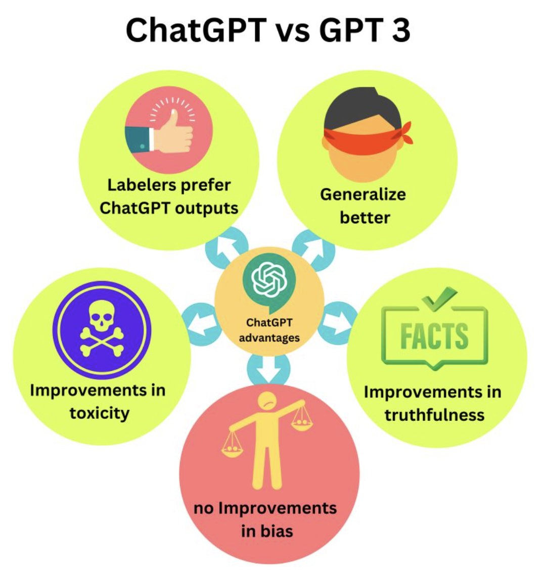
- What is it about ChatGPT we get so impressed by? GPT-3’s output is no less impressive but why does ChatGPT’s outputs feel “better”?
- The main difference between ChatGPT and GPT-3 is the tasks they are trying to solve.
- GPT-3 is mostly trying to predict the next token based on the previous tokens, including the ones from the user’s prompt, where ChatGPT tries to “follow the user’s instruction helpfully and safely”.
-
ChatGPT is trying to align to the user’s intention (https://lnkd.in/g_PA_8Xc). That is the reason InstructGPT (ChatGPT’s sibling model) with 1.3B parameters gives responses that “feel” better than GPT-33 with 175B parameters.
- ChatGPT is simply a GPT-3 model fine-tuned to human generated data with a reward mechanism to penalize responses that feel wrong to human labelers.
- They are a few advantages that emerged from that alignment training process:
- ChatGPT provides answers that are preferred over the ones generated by GPT-3
- ChatGPT generates right and informative answers twice as often as GPT-3
- ChatGPT leads to a language generation that is less toxic than GPT-3. However ChatGPT is still as biased!
- ChatGPT adapts better to different learning tasks, generalize better to unseen data, or to instructions very different from the ones found in the training data. For example, ChatGPT can answer in different languages or efficiently code, even then most of the training data is using natural English language.
-
For decades, language models were trained trying to predict sequence of words, where the key seemed to be in training to align to user’s intent. It seems conceptually obvious, but it is the first time that an alignment process is successfully applied to a language model of this scale.
- All the results presented in this post come from the InstructGPT article (https://lnkd.in/gnt9K9pu), and it is a safe assumption that those results carry to ChatGPT as well.
Generating music with text or images
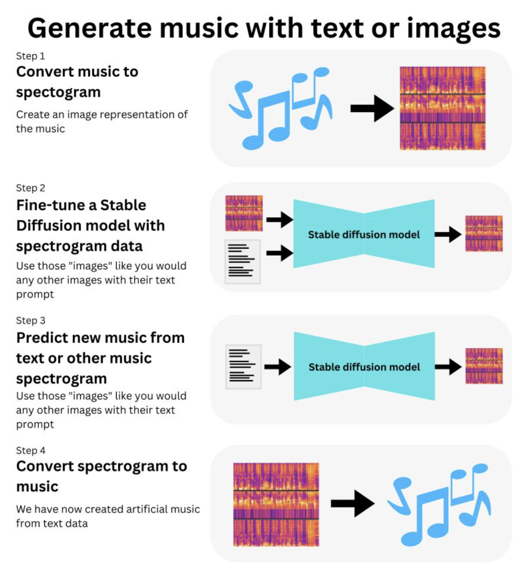
- Imagine if you could tell a ML model “play a funk bassline with a jazzy saxophone” and it would synthesize artificial music! Well actually, you don’t need to imagine, you can just use it!
-
Introducing RIFFUSION, a Stable Diffusion model trained on Spectrogram image data: https://lnkd.in/ge9_VE6t. The idea is simplistic:
- just pick a pre-trained Stable Diffusion model (https://lnkd.in/dpFheWYS)
- Take lot of musics with their text descriptions and convert that into Spectrogram image data
- Fine-tune to the Stable Diffusion model
=> you now have a model that can predict new spectrograms based on other spectrograms or text prompts. Just convert those spectrograms back to musics.
If you want more details on how to do it yourself you can follow the process here: https://lnkd.in/gpj_K-UF. I discovered this website yesterday through Alpha Signal’s weekly summary: https://alphasignal.ai/. If you to learn more about stable diffusion, you can read my LinkedIn post on it: https://lnkd.in/gxBiU9fB
Stable Diffusion
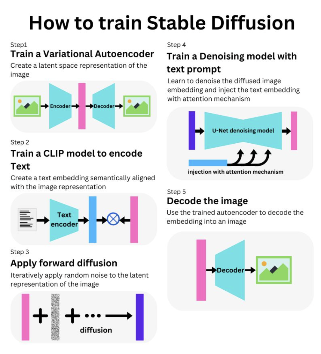
- What is STABLE DIFFUSION? It is similar to DALL-E 2 as it is a diffusion model that can be used to generate images from text prompt.
- As opposed to DALL-E 2 though, it is open source with a PyTorch implementation (https://lnkd.in/dPpjtr-d) and a pre-trained version on HuggingFace (https://lnkd.in/dpFheWYS).
-
It is trained using the LAION-5B dataset (https://lnkd.in/gewm6VEV). Stable diffusion in composed of the following sub-models:
- We have an autoencoder (https://lnkd.in/dyzQgDXH) trained by combination of a perceptual loss (https://lnkd.in/dPqz68Tp) and a patch-based adversarial objective (https://lnkd.in/dJMX3ugX).
-
With it, we can encode an image to a latent representation and decode it from it.
-
A random noise is progressively applied to the embedding (https://lnkd.in/dq2ZUKmj). A latent representation of a text prompt is learned from a CLIP alignment to the image representation (https://lnkd.in/eGNMirji).
- We then use U-Net, a convolutional network with ResNet blocks to learn to denoise the diffused embedding (https://lnkd.in/dBppaqVK).
- The textual information is injected through cross-attention layers through the network (https://lnkd.in/dWsrEkpD).
-
The resulting denoised image is then decoded by the autoencoder decoder.
- The process is described here: https://lnkd.in/d4NijqmG and one of the best explanation on Stable Diffusion here: https://lnkd.in/dpWMm_kS. Fun model!
How to generate animation with Stable Diffusion
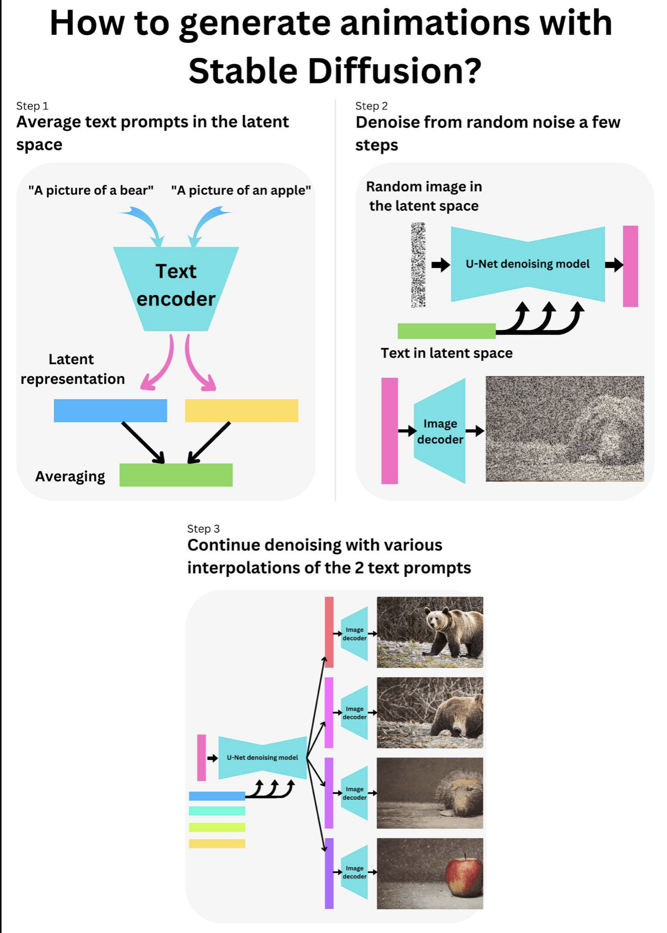
But how do we generate those cool animations with STABLE DIFFUSION? Check out the one I did in Replicate: https://replicate.com/p/uzj2czjjzradtjcrzet6yfqdkq. Those animations are mostly due to the fact that it is easy to interpolate between 2 images or 2 text prompts in the latent space (embedding representations). The DALL-E 2 article explains that pretty well: https://arxiv.org/pdf/2204.06125.pdf. You need a start and end prompt. I chose “A picture of a bear” and “A picture of an apple”. You then encode those texts in the latent space using the text encoder of the CLIP model (https://openai.com/blog/clip/), and you use the interpolation between the 2 text prompts to guide the denoising process of a random image for a few steps. This is just to anchor the denoising process in between the 2 prompts such that the animation is less jumpy. You then create as many intermediary interpolations between the 2 prompts as you need frames in your animation, and continue the denoising process until getting clean images. If you need smoother animations, you simply interpolate between the generated images in the latent space. I have had a lot of fun playing with Andreas Jansson’s implementation of animations with Stable Diffusion: https://replicate.com/andreasjansson/stable-diffusion-animation. He is using the pretrained model on Hugging Face (https://huggingface.co/…/huggingface…/diffuse-the-rest). You can learn more about it my Newsletter: https://newsletter.TheAiEdge.io/ —- Follow me for more Machine Learning content!
🚀 Stable diffusion stands out among diffusion models, Here is Why.
Stable Diffusion (SD) offers Knobs to trade-off Speed, Sample quality and Guidance for high fidelity.
Here are the ideas that made those properties possible:
→ Latent diffusion: Originally Diffusion models operated on Pixel space, hence computationally exorbitant, Latent diffusion projects images to a Latent space.
This means a immaculate tradeoff between sample quality and speed. Hence SD lends itself to high quality 512x512 samples in acceptable speeds. Canva introduced text to image using SD, recently.
→ Non-Markovian noise scheduling: Diffusion models noise and de-noise images along number of time steps . Akin to sequence modelling like in RNNs.
But RNNs are better than Markov models for sequence modelling because they defy markov porperty and can learn long range relationships.
Honouring the same tradition SD uses DDIM (and cousins), a set of Non-markovian noising schedulers to accelerates sampling as opposed to slower markovian DDPM.
SD exposes num_inference_steps for this, more the steps, better the image quality.
→ (Noise Conditional) Score-Based Modelling:
Typically likelihood models like VAE, Flow based, EBMs and implicitly generative models like GANs have multiple challenges.
Latter is unstable (owing to mode collapse) which inspite of adversarial training trades off diversity for quality.
Former tries to model the probability density (or mass) function of the distribution of the data which quickly becomes intractable mathematically. Hence score based models offers a perfect side stepping, to model a tractable score function using schedules of noise and measures performance by score matching techniques like Fischer’s divergence.
→ Classifier free guidance: Originally diffusion was aimed at unconditional generation. To condition the generation with text, guided diffusion was introduced, it was done using an ancillary classifier model that trades-off diversity of samples for fidelity aka faithfulness to the prompt.
Idea is to use the gradient of the classifier model trained on noisy images to guide demonising during inferences.
But thanks to Jonathan Ho, he introduced classifier free guidance (CFG), SD uses this technique and exposes a single scalar parameter called “guidance scale”. CFG removes the need for one extra model. DALL-E(CLIP), GLIDE and ImageGen (T5) all use a classier based guidance.
On the downside, CFG is one of the potential reasons why you need to write elaborate prompts for SD and but that’s not the case with DALL-E.
ML Youtube channels
Sometime we just need to sit back and relax watching videos! Here are great YouTube channels to learn Machine Learning from. Enjoy:
- What’s AI by Louis Bouchard: https://lnkd.in/euVngxvQ
- Abhishek Thakur (Practical videos, Talks) : https://lnkd.in/eTPrcvEN
- Ahlad Kumar (Deep learning, Theoretical): https://lnkd.in/eVGxpXfw
- Aladdin Persson (PyTorch, TensorFlow): https://lnkd.in/e29966pV
- Andreas Mueller: https://lnkd.in/eQYM3WyC
- Data School (Python, Machine learning, Theoretical): https://lnkd.in/eXEjf27Q
- Connor Shorten (Theoretical): https://lnkd.in/ejdwwyzq
- Jeremy Howard (Deep learning, Theoretical): https://lnkd.in/ec3DGa7g
- Rasa (Rasa, AI, NLP): https://lnkd.in/ehUe-qPE
- Yannic Kilcher (NLP, Machine learning, Deep learning, Theoretical): https://lnkd.in/ebRk-bMB
- OpenAI (NLP, Machine learning, AI): https://lnkd.in/eWvCKiqz
- Two Minute Papers (Machine Learning and AI Research, Scientific Papers): https://lnkd.in/eQY_5_SV
- Machine Learnia (Machine Learning, Scikit Learn, Python): https://lnkd.in/enFTrVh9
- Mark Saroufim (Machine Learning Engineering, Practical videos, Books review): https://lnkd.in/ez32nFS5
- sentdex (Python for AI and Finance): https://lnkd.in/eMsdgVbS
I found that curated list of YouTubers on this awesome repo: https://lnkd.in/eVgmFN8Y. That repo has similar lists for many other software skills, so make sure to check it out.
DALLE-2
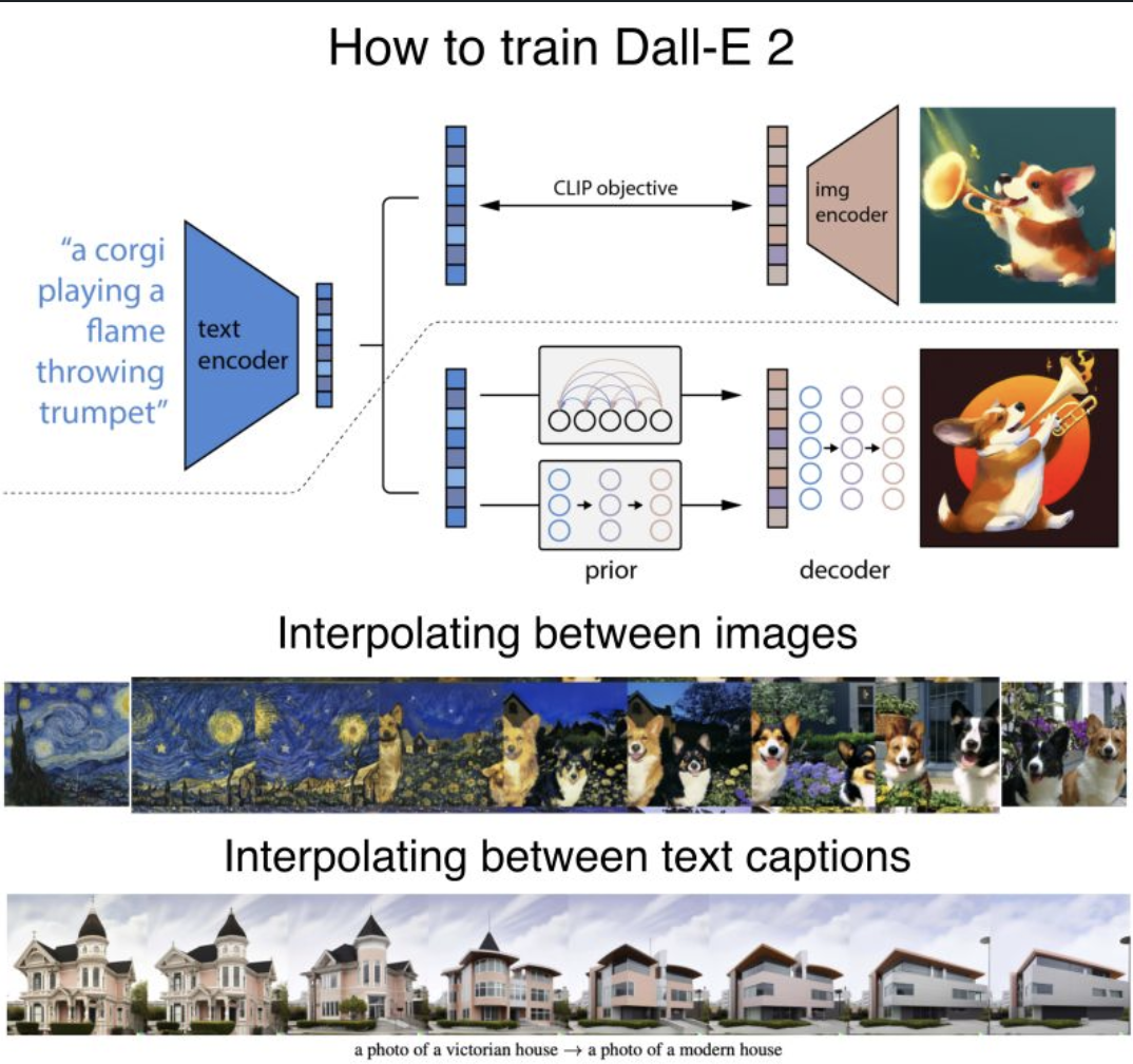
- How does DALL-E 2 work? DALL-E 2 generates non-deterministic images from text data.
-
It is basically a combination of 2 models: a CLIP model that predicts image from text and a diffusion model that predicts non-deterministically images from image embeddings.
- First, they train a Contrastive Language-Image Pre-training (CLIP) model that predicts images with text inputs: https://lnkd.in/eGNMirji, https://lnkd.in/eHbmBb2t.
- By training that model, they obtain a CLIP text embedding T and an image embedding E.
- The second model is a Diffusion model that takes an image embedding E and predicts non-deterministic images: https://lnkd.in/erwcgzzz, https://lnkd.in/eC3FRMMq
-> Piping those 2 models together, a text caption can be used to predict an image embedding E that in turn can be used to predict non deterministic images.
- Learning those embeddings lead to interesting properties.
- For example, we can take 2 images and their resulting embeddings E1 and E2 and continuously interpolate between the 2 embeddings in the latent space.
- This results in having the capability to create new images that seem to have their styled mixed together with a lot of control.
- We can also do a very similar thing with the text embedding by having 2 text captions and their resulting embeddings T1 and T2.
-
By interpolating between those 2 again in the latent space, we can continuously create images that capture the intermediate meaning of the 2 captions.
- The results are honestly baffling! I think with models like GAN and now Dall-E, we have entered an era of Machine Learning where engineers are able to put together specialized models together in a creative way to achieve what doesn’t look like what we used to call “Machine Learning” anymore.
- You can find the Dall-E 2 article here: https://lnkd.in/evk2QQWd, https://lnkd.in/e6HDhscP, and you can compare it to Dall-E 1: https://lnkd.in/etpBqDjK. If you want to play with it, you can try the OpenAI API: https://lnkd.in/ePSKNNWN
Forward-Forward Algorithm
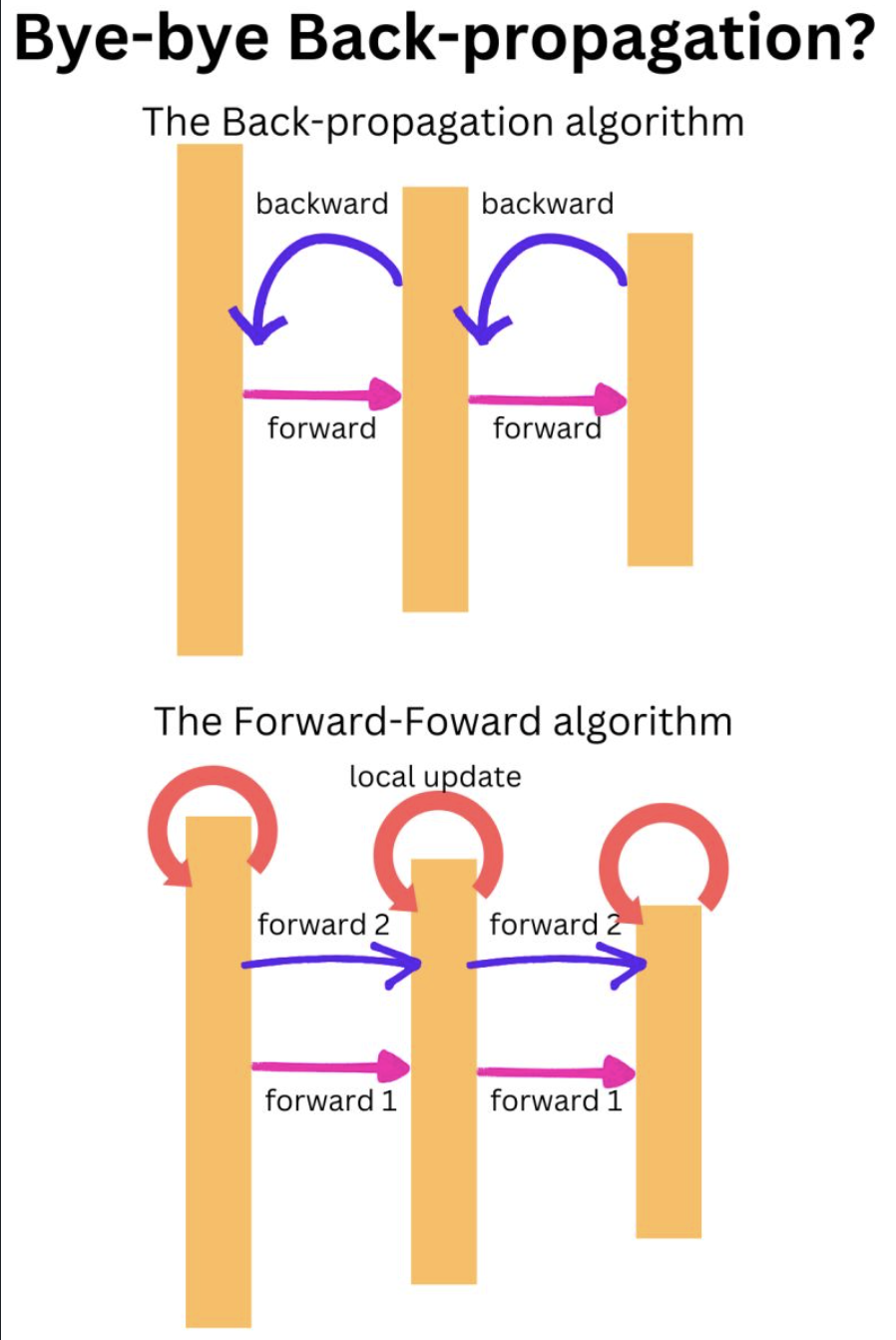
- We may not need the BACK PROPAGATION algorithm anymore! Hinton is presenting results on the Forward-Forward algorithm: https://lnkd.in/gkU_tqNz.
- The first forward pass in done with real data and the second forward data is done with “negative data” and the weights are learned by computing a local gradient. It seems to have 2 advantages: first, it to work well enough on a few problems for now, and second, there seems to be possible to separate the 2 forward learning phases.
-
Imagine if you could train the forward passes and the backward passes at different points in time. I will need time to build a good intuition on that one!
- At each layer, the local “target” P is the sum of the square of the activation functions squeezed in the probability space by a logistic function and a threshold.
- The real data should lead to P ~ 1 (activations above the threshold) and the negative data should lead to P ~ 0 (activations below the threshold).
-
The gradient can be computed locally and the weights can be updated using that “local classification” process.
- For image classification for example, the real data could be a pair of image X and a target y (X, y), where the negative data can be an image X paired with a random target y’ (X, y’).
You can find a PyTorch implementation of the Forward-Forward algorithm in this repo: https://lnkd.in/g58uv7TK. I am looking forward to see more experimental results on that one. I have a feeling that this is going to change Deep Learning as we know it!
ChatGPT
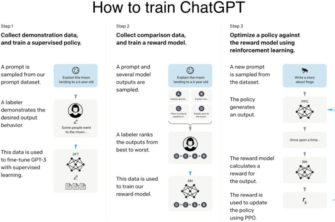
- Do you know how ChatGPT was trained? ChatGPT is “simply” a fined-tuned GPT-3 model with a surprisingly small amount of data!
-
Moreover, ChatGPT is using 1.3B parameters where GPT-3 uses 175B parameters! It is first fine-tuned with supervised learning and then further fine-tuned with reinforcement learning. They hired 40 human labelers to generate the training data. Let’s dig into it!
- First, they started by a pre-trained GPT-3 model trained on a broad distribution of Internet data (https://lnkd.in/gAUtxvrM).
- Then sampled typical human prompts used for GPT collected from the OpenAI website and asked labelers and customers to write down the correct output.
-
They fine-tuned the model with 12,725 labeled data.
- Then, they sampled human prompts and generated multiple outputs from the model for each of the prompt. A labeler is then asked to rank those outputs.
-
The resulting data is used to train a Reward model (https://lnkd.in/gdrzdWu3) with 33,207 prompts and ~10 times more training samples using different combination of the ranked outputs.
- We then sample more human prompts and they are used to fine-tuned the supervised fine-tuned model with Proximal Policy Optimization algorithm (PPO), a Reinforcement Learning algorithm (https://lnkd.in/gsDTWtga).
- The prompt is fed to the PPO model, the Reward model generates a reward value, and the PPO model is iteratively fine-tuned using the rewards and the prompts using 31,144 prompts data.
This process is fully described in here: https://lnkd.in/gnt9K9pu. The paper actually details a model called InstructGPT which is described by OpenAI as a “sibling model” to ChatGPT, so the numbers shown above may be slightly different from the exact ones used for ChatGPT.
What is it about ChatGPT we get so impressed by? GPT-3’s output is no less impressive but why does ChatGPT’s outputs feel “better”? The main difference between ChatGPT and GPT-3 is the tasks they are trying to solve. GPT-3 is mostly trying to predict the next token based on the previous tokens, including the ones from the user’s prompt, where ChatGPT tries to “follow the user’s instruction helpfully and safely”. ChatGPT is trying to align to the user’s intention (alignment research). That is the reason InstructGPT (ChatGPT’s sibling model) with 1.3B parameters give responses that “feel” better than GPT-3 with 175B parameters.
The Training
ChatGPT vs GPT-3
The Training ChatGPT is “simply” a fined-tuned GPT-3 model with a surprisingly small amount of data! It is first fine-tuned with supervised learning and then further fine-tuned with reinforcement learning. In the case of InstructGPT, they hired 40 human labelers to generate the training data. Let’s dig into it (the following numbers were the ones used for InstructGPT)!
First, they started by a pre-trained GPT-3 model trained on a broad distribution of Internet data (GPT-3 article). Then sampled typical human prompts used for GPT-3 collected from the OpenAI website and asked labelers and customers to write down the correct outputs. They fine-tuned the model in a supervised learning manner using 12,725 labeled data point.
Then, they sampled human prompts and generated multiple outputs from the model. A labeler is then asked to rank those outputs. The resulting data is used to train a Reward model (https://arxiv.org/pdf/2009.01325.pdf) with 33,207 prompts and ~10 times more training samples using different combinations of the ranked outputs.
They then sampled more human prompts and they were used to fine-tuned the supervised fine-tuned model with Proximal Policy Optimization algorithm (PPO) (https://arxiv.org/pdf/1707.06347.pdf), a Reinforcement Learning algorithm. The prompt is fed to the PPO model, the Reward model generates a reward value, and the PPO model is iteratively fine-tuned using the rewards and the prompts using 31,144 prompts data.
ML for Ads Ranking RecSys
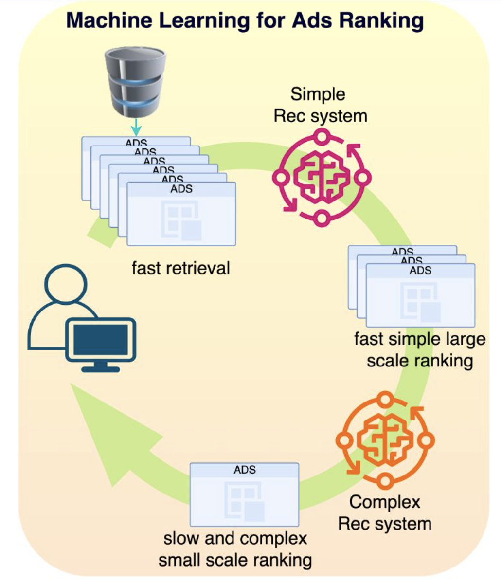
At Meta, we were using many different paradigms of Recommendation Engines for ADS RANKING. Conceptually, a recommender system is simple: you take a set of features for a user U and a set of features for an item I along with features C capturing the context at the time of the recommendation (time of the day, weekend / week day, …), and you match those features to an affinity event (e.g. did the user click on the ad or not): click or not = F(U, I, C).
-In the early days they started with Gradient Boosting models. Those models are good with dense features (e.g. age, gender, number of clicks in the last month, …) but very bad with sparse features (page Id, user Id, Ad Id, …). By the way, we often talk of the superiority of Tree based models for tabular data, well this is a real exception to the rule! Those sparse features are categorical features with literally billions of categories and very few sample events. For example, consider the time series of sequence of pages visited by a user, how do you build features to capture that information? That is why they moved to Deep Learning little by little where a page Id becomes a vector in an embedding and a sequence of page Ids can be encoded by transformers as a simple vector. And even with little information on that page, the embedding can provide a good guess by using similar user interactions to other pages.
-Typical models we were using were Multi-task learning (https://lnkd.in/gVZ7HrUz), Mixture of experts (https://lnkd.in/dE6XZvJx) or Multi-towers models (https://lnkd.in/gPZ-GfRS). In Ads Ranking, the ranking happens in stages: first you select a sub-universe of ads (let’s say 1M ads) that relate to the user (very fast retrieval), then you select a subset of those ads (let’s say 1000 Ads) with a simple model (fast inference) and then you use a very complex model (slow inference) to rank the resulting ads as accurately as possible. The top ranked ad will be the one you see on your screen. We also used MIMO (multi-inputs multi-outputs) models to simultaneously train the simple and complex models for efficient 2 stages ranking.
-I cannot think of a model type that capture better the success of ML in our societies. Google search, Google or Facebook Ads, Youtube suggestions, Netflix movie suggestions, Amazon products search, … are all the results of decades of research in recommender systems and are all top drivers of the cash flows for those companies.
Is PageRank still used at Google
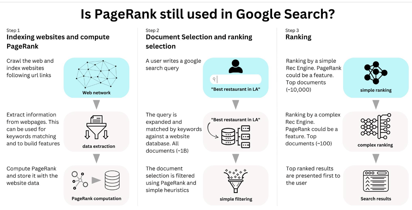
Is PageRank still used as part of Google Search? Yes we know it is as we can see in the list of systems that are currently in use: https://developers.google.com/…/ranking-systems-guide. PageRank is a metric of importance of a website as measured by how connected that website is to others (https://snap.stanford.edu/…/cs224w…/Brin98Anatomy.pdf). It used to be the main way websites were ranked in Google Search, leading to its success at the time, but now searches are personalized where PageRank is a global metric. We don’t know how it is used, but we can pretty much guess!
-
A Google search happens in stages. First, the search query is expanded and used to perform an initial Document Selection. This document selection is driven by keywords matching in a database. If I type today “google search”, Google tells me there are about 25B results related to my search.
-
Then results go through a set of Recommender engines. There is most likely a simple Rec Engine first ranking a large amount of documents (maybe 100,000 or 10,000 documents) and a complex one refining the ranking of the top ranked documents (maybe 100 or 1000). Who cares about the quality of the ranking for the documents far in the list of documents! The websites are probably already ranked by PageRank in the initial document selection as it can be computed at indexing time. There is no need to send all 25B documents to the first Rec engine, and PageRank is most likely used as a cutoff to send a small subset.
-
However it is unlikely that PageRank is the only cutoff parameter as some websites would never get discovered. I would expect some simple geolocalization and context matching metrics as well as randomization to be used as well.
-
At this point the ranking becomes personalized, and user data becomes the main factor, but PageRank is likely to still be used as a feature for all the successive Rec Engines used in the search pipeline.
Obviously those are educated guesses as those information are not public. You can learn more about it my Newsletter: https://newsletter.TheAiEdge.io/
CLIP
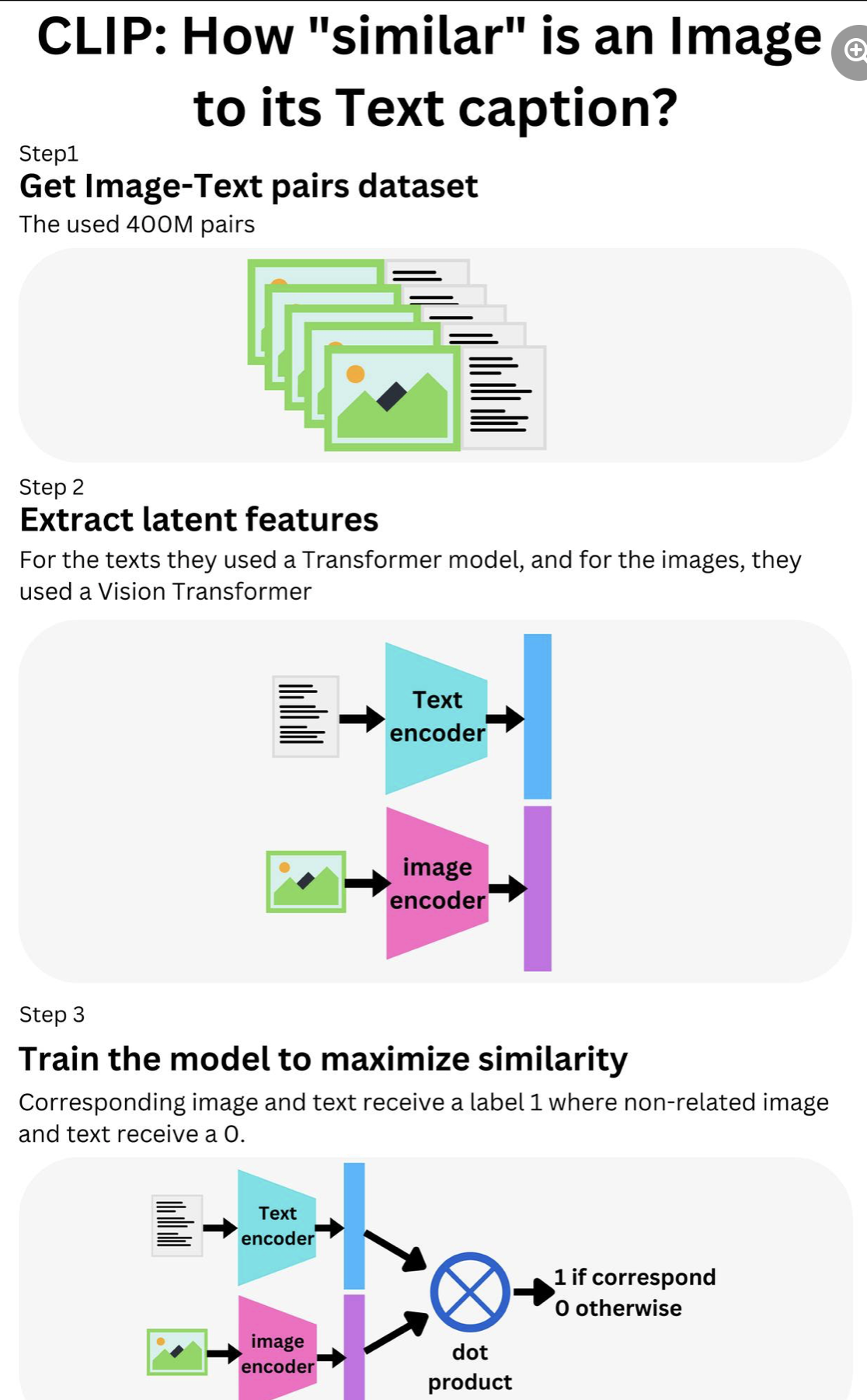
How would you know if an image is “similar” to its text caption? Conceptually, you could “simply’’ measure the cosine similarity between the image and the text. That is the idea behind CLIP (Contrastive Language-Image Pretraining: https://openai.com/blog/clip/), the OpenAI algorithm underlying Dall-E 2 (https://arxiv.org/pdf/2204.06125.pdf) and Stable Diffusion (https://arxiv.org/pdf/2112.10752.pdf). An intermediate latent vector representation of the image and the text is learned such that a high value of the dot product is indicative of high similarity. First, they created a dataset of 400M pairs (image, text) from publicly available datasets on the internet. Then they used a 63M parameters Transformer model (A small GPT-2 like model: https://cdn.openai.com/…/language_models_are…) to extract the text features T and a Vision transformer (https://arxiv.org/pdf/2010.11929.pdf) to extract the image features I. The resulting vectors are further transformed such that the text and image vectors have the same size. With N (image, text) pairs, we can generate N^2 - N pairs where the image does not correspond to the text caption. They then take the normalized dot product (cosine similarity) between T and I. If the text corresponds to the image, the model receives a label 1 and 0 otherwise, such that the model learns that corresponding image and text should generate a dot product close to 1. This model has a lot of applications in zero-shot learning! In typical image classification, we feed the model with an image, and the model provides a guess from a set of predefined text labels used during the supervised training. But with CLIP, we can provide the set of text labels we want the model to classify the image into without having to retrain the model because the model will try to gauge the similarity between those labels and the image. We can virtually build an infinite amount of Image classifiers by just switching the text labels! The article ( https://arxiv.org/pdf/2103.00020.pdf) showcases the robustness of CLIP to generalize to different learning tasks without the need to retrain the model. In my opinion, this adaptability of ML models shows how much closer we are from true Artificial Intelligence! CLIP is an open-source project (https://github.com/openai/CLIP), so make sure to try it.
Quick Feature Selection Method
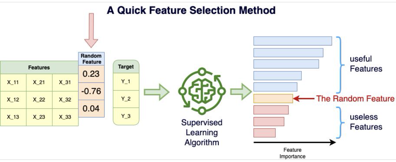
This is a technique I like to perform a quick FEATURE SELECTION for Machine Learning applications. I tend to call it the “Random Bar” method! Let’s assume you have a feature set X and a target Y. Let’s create a random vector V (for example np.random.normal(size=(1, 100))) and append that vector as a new feature to X: X’ = [X, V] X’ is just the original feature set with additionally the new random feature. Keep in mind that this new feature cannot possibly help to predict the target Y since it is random! Now, take that data (X’, Y) and train a Supervised Learning algorithm with a Feature Importance measure that is relevant for you application. Intuitively, the mean entropy gain per split of tree based algorithms (Random Forest, Xgboost, …) is a convincing measure of feature importance to me. The statistical fluctuation of the data is such that even the random feature will be attributed a non-zero feature importance by the algorithm, but we know it is artificial. Any feature with a lower feature importance than the random feature has to be useless to predict the target and the features with a higher feature importance are at least better than random noise at predicting the target. This is especially useful if you have thousands of features and you want to weed out quickly the ones that won’t have any impact in the learning process. This is also a method that can be used for highly non-linear data as opposed to LASSO (for example) that tends to only understand linear relationships in the data. The random feature is a “Random Bar” because this is the minimum bar a feature needs to beat to be a part of the potentially useful features set. Now it doesn’t mean there are not additional features that could be beneficial to further remove to optimize your model. Do you know if this method has a more jargon-y name? What is your favorite feature selection method?
Overfitting
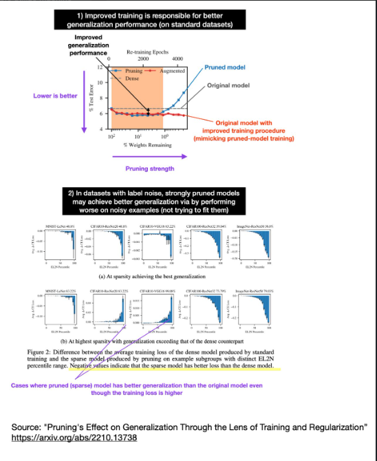
After sharing various methods that reduce overfitting yesterday, I found some intriguing new research studying the effect of pruning on the generalization performance.
It’s been known that pruning (producing smaller models) can improve generalization performance. At the same time, we also know that larger, overparameterized models can improve generalization performance (e.g., see double decent and grokking).
So, how can we reconcile the observation that pruned models can exhibit better generalization performance with contradictory observations from double decent and grokking studies? Researchers recently showed that the reduction of overfitting due to pruning could be partly explained by the improved training process[. Pruning involves more extended training periods and a replay of learning rate schedules that are partly responsible for improved generalization performance.
On noisy datasets, however, the generalization performance improvements due to pruning can be explained by a larger loss on noisy training examples. Why is a larger loss on noisy training examples better? Presumably because the pruned models don’t try to fit these noisy examples, which adds a regularizing effect – this is somewhat similar to reducing the width of the layers.
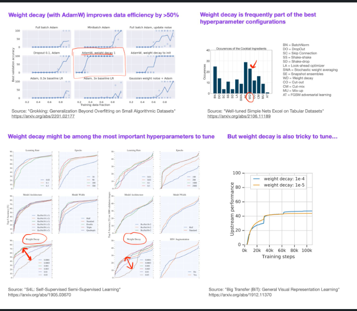
- Suppose your deep neural network suffers from overfitting. In that case, there is a large pool of techniques and approaches to choose from (I separated the most common ones into dataset and model perspectives two days ago).
Now, the follow-up question is, which of the techniques gives you the most gain? Weight decay (with AdamW) is definitely one you should consider in your regularization cocktail.
In the figure below, I summarized 4 references that discuss different aspects of weight decay and its effects on overfitting.
Pruning
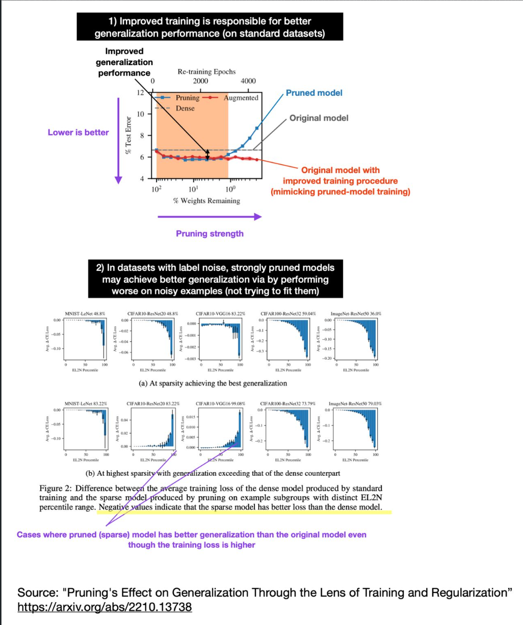
After sharing various methods that reduce overfitting yesterday, I found some intriguing new research studying the effect of pruning on the generalization performance.
It’s been known that pruning (producing smaller models) can improve generalization performance. At the same time, we also know that larger, overparameterized models can improve generalization performance (e.g., see double decent and grokking).
So, how can we reconcile the observation that pruned models can exhibit better generalization performance with contradictory observations from double decent and grokking studies? Researchers recently showed that the reduction of overfitting due to pruning could be partly explained by the improved training process[. Pruning involves more extended training periods and a replay of learning rate schedules that are partly responsible for improved generalization performance.
On noisy datasets, however, the generalization performance improvements due to pruning can be explained by a larger loss on noisy training examples. Why is a larger loss on noisy training examples better? Presumably because the pruned models don’t try to fit these noisy examples, which adds a regularizing effect – this is somewhat similar to reducing the width of the layers.
Information Retrieval Metrics
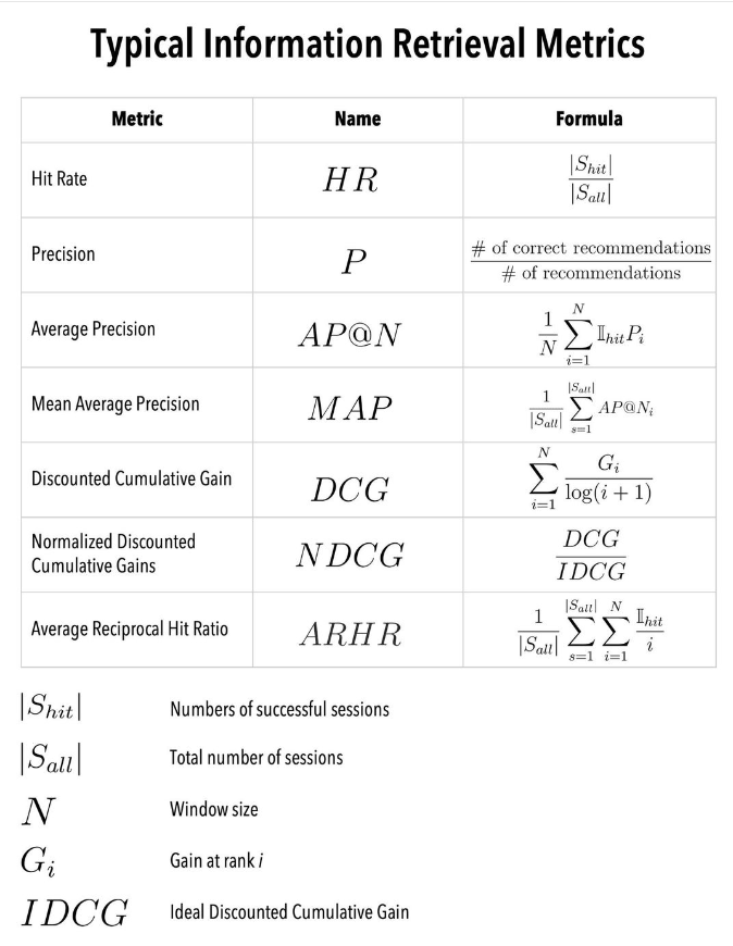
I may be wrong, but I think it is quite unlikely that Google ML ENGINEERS are using typical information retrieval metrics to assess the offline performance of the ML classifiers used within Google Search or similar search engine! There are ~3.5 billion searches per day, with each search generating a lot of positive and negative samples. If you train a classifier on that data, you probably want to spam at least a few days of data if not more. It is an extremely class imbalanced problem, so you’ll probably want to downsample the majority class for the computation to be manageable. That is still tens of billions of samples for each model development at least!
A metric like Normalized Discounted Cumulative Gain (NDCG) requires the concept of relevance (gain) to part of the data. That can be achieved with manual labeling but that is NOT going to be manageable on billions of samples. Metrics like Mean Reciprocal Rank (MRR) or Mean Average Precision (MAP) requires to know the true rank of the sample, meaning if I assess a classifier on a validation data, the predicted rank per search session is not going to be meaningful if we downsampled the data, and the metrics will be extremely dependent on the specific sampling scheme. We could imagine that we downsample the number of sessions instead of the majority class, but this forces us to only keep the top samples shown by the algorithms. That seems unwise since this will prevent ML engineers from experimenting with new sampling methods in future developments and the models will never see very negative samples, which is a bit problematic if we want to build an accurate model. The same problem occurs with a metric like Hit rate, since you need a window size.
If you order the search results by the probability of click provided by the classifier, the log-loss (or cross entropy) is a completely acceptable ranking metric. It is a point-wise metric, which means it doesn’t require us to know the predicted rank of the sample to compute a meaningful value. The probability itself will be biased by the false class distribution coming from the downsampling, but this can be corrected by recalibrating the probability p using the simple formula: p’ = p / (p + (1-p) * s), where s is the negative sampling rate (https://eva.fing.edu.uy/…/Elkan_2001_The_foundations_of…).
With a probability metric such as the log-loss, I expect more freedom for the ML engineers to experiment with new techniques. For example, in the case of search engines, we could label with 1 the clicked links and 0 the non-clicked links, but you could also imagine that the negative samples are only sampled from unsuccessful sessions (where the users did not find the right link). In a successful session, the non-clicked links are not really “bad”, they are just less interesting to the user. To be able to assess across models and teams, it might be useful to use the normalized entropy metric (https://deychak.github.io/normalized-cross-entropy) as anything above 1 is worse than random.
XGBoost
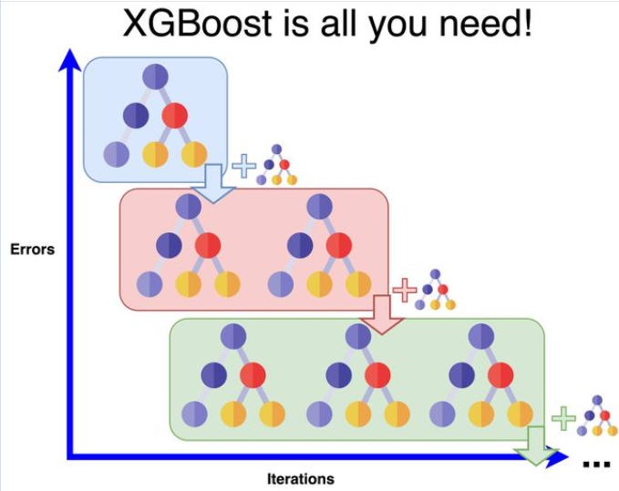
“XGBoost is ALL you need!” Well, it is true until it is not. Algorithms like Linear Regression have their number of degrees of freedom (d.o.f. - complexity) scaling with the number of features O(M). In practice, this means that their ability to learn from the data will plateau in the regime N » M where N is the number of samples (typically large data sets). They have a high bias but a low variance and as such they are well adapted to the N > M regime. In the N < M regime, L1 regularization becomes necessary to learn the relevant features and zero-out the noise (think about having more unknowns than equations to solve a set of linear equations). Naive Bayes d.o.f. scales as O(C x M) (or O(M)depending on the implementation) where C is the number categories the features are discretized into. O(C) = O(N) in theory but not really in practice. This makes it a lower bias algorithm than LR but it is a product ensemble of univariate models and ignores the feature interactions (as LR does) preventing it from further improvements.
A tree in its unregularized form, is a low bias (you can overfit the data to death), with d.o.f scaling as O(N), but high variance (deep trees don’t generalize well). But because a tree can reduce its complexity as much as needed, it can work in the regime N < M by simply selecting the necessary features. A Random Forest is therefore a low bias algorithm but the ensemble averages away the variance (but deeper trees call for more trees) and it doesn’t overfit on the number of trees (Theorem 1.2 https://www.stat.berkeley.edu/~breiman/randomforest2001.pdf), so it is a lower variance algorithm. The homogenous learning (the trees tend to be similar) tends to limit its ability to learn on too much data.
XGBoost is the first (to my knowledge) tree algorithm to mathematically formalize regularization in a tree (eq. 2 https://arxiv.org/pdf/1603.02754.pdf). It is a low bias and high variance (due to the boosting mechanism) and is therefore adapted to large data scales. The GBM Boosting mechanism ensures a more heterogenous learning than RF and therefore adapts better to larger scales. The optimal regularization ensures higher quality trees as weak learners than in RF and tends to be more robust to overfitting than RF.
In the regime N » M, only low bias algorithms make sense with d.o.f. scaling as O(N). That includes algorithms like GBM, RF, Neural Networks, SVM (gaussian), KNN,… SVM has a training time complexity of O(N^3) (unmanageable!) and KNN is bad at understanding what is an important feature and has dimensionality errors scaling as O(M). Neural Networks are known to underperform compared to XGBoost on tabular data.
So, if you are working on large data, XGBoost MAY be all you need! But make sure to prove it to yourself. The no Free-Lunch Theorem doesn’t mean we cannot understand our algorithms and build an intuition on what are the best use cases to use them!
—
Follow me for more Machine Learning content!
#machinelearning #datascience #XGBoost
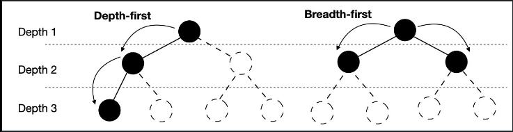
A question often arises when teaching is how XGBoost and LightGBM differ. The short fun-fact summary is that the tree-building algorithms are a tad different.
XGBoost’s trees are based on breadth-first search, comparing different features at each node.
LightGBM performs depth-first search, focusing on a single feature at a time and growing the tree from there.
1) BFS : Is memory intensive, take more time to execute. Likely to underfit if stop early. To control this I guess some package has ability to convert that to Uniform Cost search I believe it will work well where dataset contains more categorical independent variable
2) DFS: Require less memory as compared to BFS. Likely to overfit and stuck in local minima situation. To control this I guess some package has ability to convert that to Depth Limit Search. I believe DFS will work well in number input features.
Data Parallelization by Sebastian Raschka
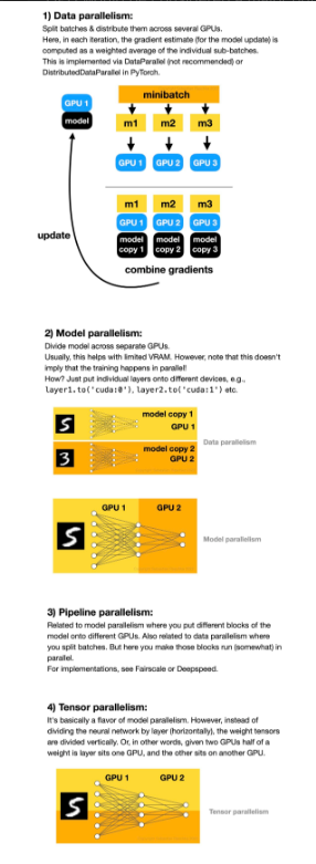
When I started grad school, training deep neural networks on a GPU was something special – it was both tricky to do and awesome when it worked).
The world has moved on since then! Nowadays, training a model on a single GPU would be considered a major bottleneck.
Here is a quick overview of the 4 different paradigms for multi-GPU training.
1) Data parallelism 2) Model parallelism 3) Pipeline parallelism 4) Tensor parallelism
Top 5 basic checks when trianing deep learning models
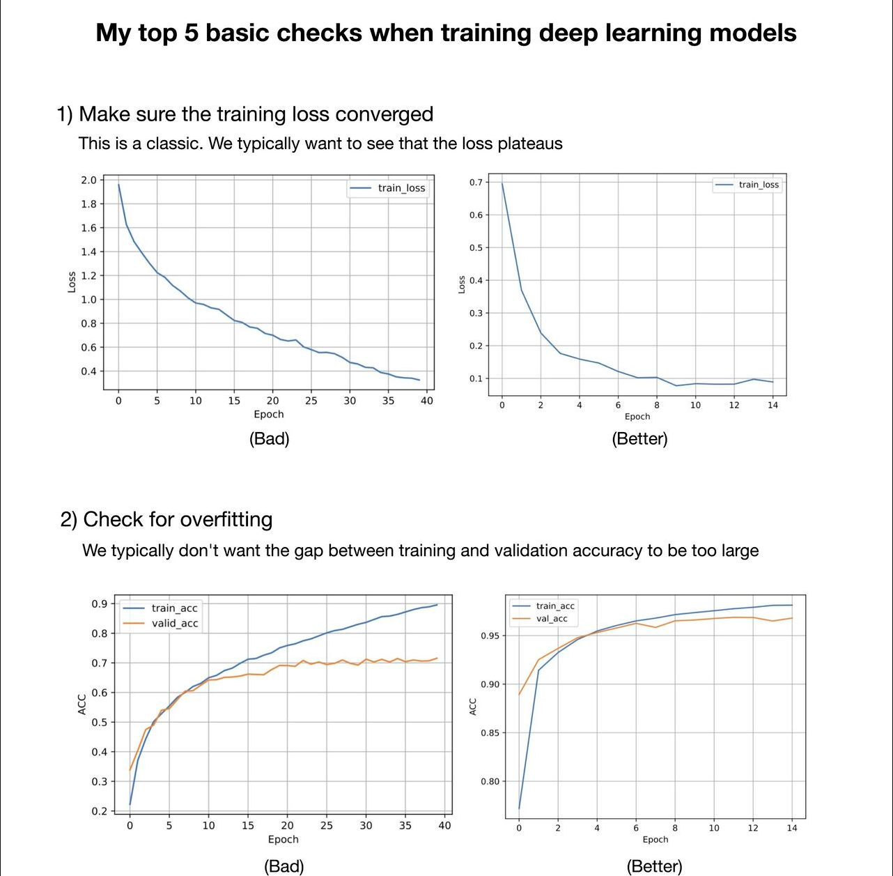
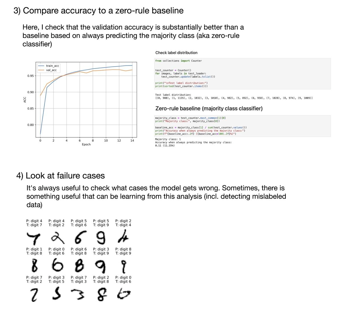
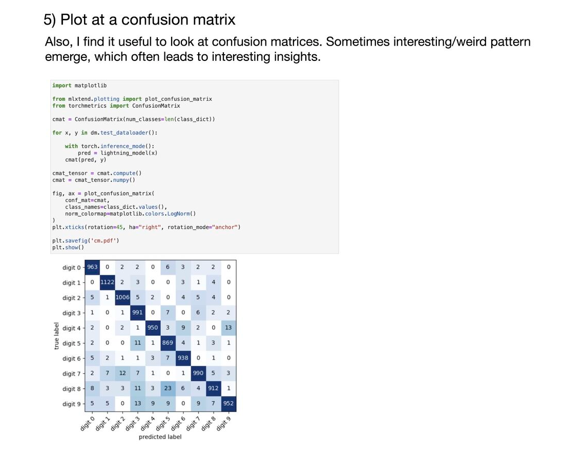
What are some of the basic things you should watch out for when training deep neural networks? Here are my top 5:
1) Make sure training loss converged 2) Check for overfitting 3) Compare accuracy to a zero-rule baseline 4) Look at failure cases 5) Plot at a confusion matrix 6) Make sure your model is able to overfit to a small dataset (like 1000 examples) or a single minibatch. (Tip 3 from Andrej Karpathy’s “A Recipe for Training Neural Networks” https://lnkd.in/gvfgqxTQ) 7) Check whether layers have converged to a good alpha (e.g., using weightwatcher). See https://lnkd.in/gHDHDXAu 8) Check how confident your model is on out-of-distribution data (a common problem for neural nets); one out of many papers on this topic: https://lnkd.in/gsjSVYcd 9) Apply your model to new data from the application domain (e.g., if you train a handwritten digit classifier, try your own handwritten digits)
A list of 5 techniques to optimize deep neural network model performance during inference
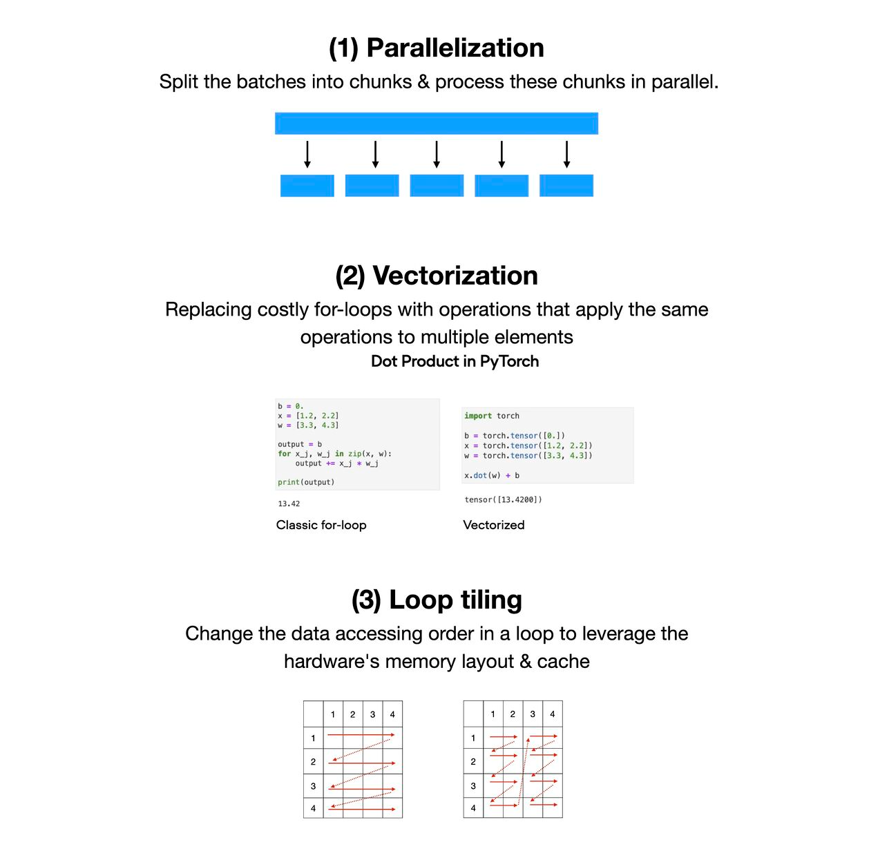
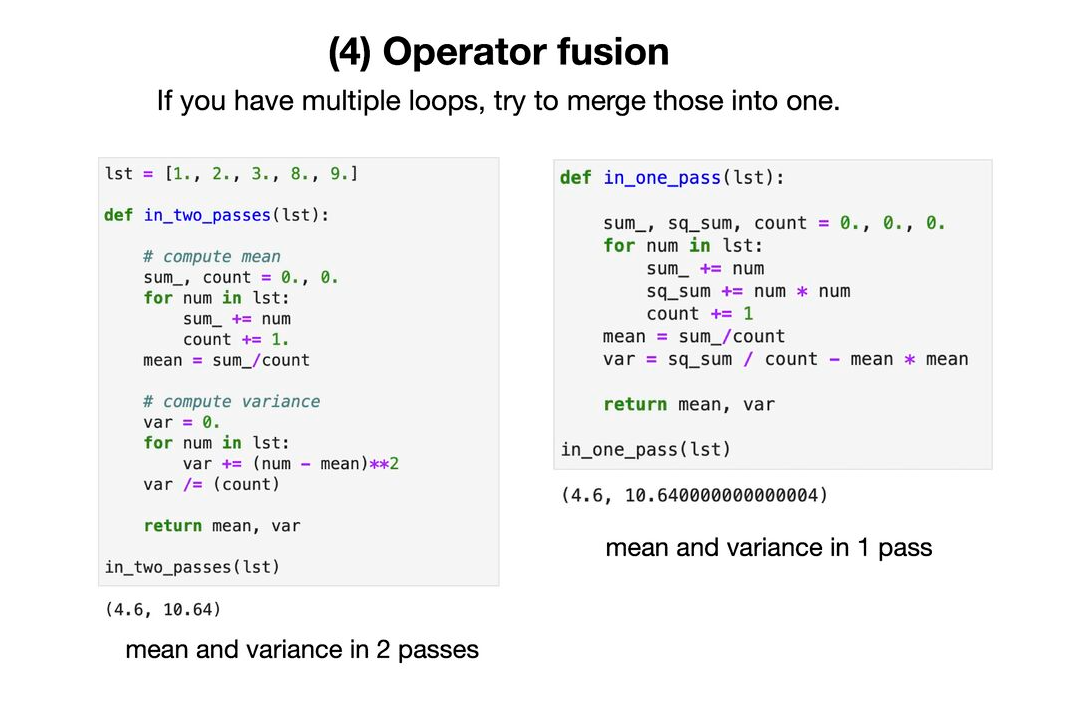
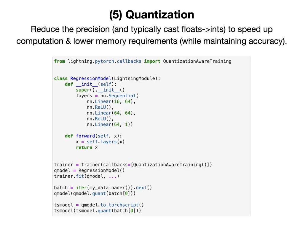
Links for MLOPS
Courses:
- Made With ML: https://madewithml.com/
- Coursera - DeepLearning.AI MLOps specialization: https://lnkd.in/gVrxJqQS
- Coursera - Google MLE certificate: https://lnkd.in/gVNNpzzR
- MLOps Zoomcamp: https://lnkd.in/gt2QH7sz
- Berkeley Full Stack Deep Learning: https://lnkd.in/gG8jR2Vg
- Udemy - Deployment of Machine Learning Models: https://lnkd.in/g7TpQ_dM
- Udemy - MLOps Fundamentals CI/CD/CT: https://lnkd.in/gkW9Gkrj
- Udemy - Testing and Monitoring Machine Learning Model Deployments: https://lnkd.in/g4qAw9Hq
- MLOps Certification Training: https://lnkd.in/guRq627D
- MLOps Engineering on AWS: https://lnkd.in/g-tnpKuY
- AWS Machine Learning University: https://lnkd.in/g-jjMk3Q
- EdX - MLOps with AWS: https://lnkd.in/gYE37jDN
- MLOps Course Certification: https://lnkd.in/gDGUXPR7
- GCP MLOps Fundamentals: https://lnkd.in/geNjGNyP
- Stanford MLSys Seminar Series: https://lnkd.in/gdNWPceY
- DataRobot MLOps Starter: https://lnkd.in/gMQYSitX
- Udacity - Become a Machine Learning Engineer for Microsoft Azure: https://lnkd.in/garedV7K
- LinkedIn - Applied Machine Learning Foundations: https://lnkd.in/ghWPcHHq
- Unifying MLOps at Microsoft: https://lnkd.in/gsKyb3Dq
Books:
- Machine Learning Engineering: https://lnkd.in/gjyw35fh
- Introducing MLOps: https://lnkd.in/gZzh_cYz
- What Is MLOps?: https://lnkd.in/g_vgYKMh
- Practical MLOps: https://lnkd.in/gbGnj7ss
- Reliable Machine Learning: https://lnkd.in/gCvje923
- Designing Machine Learning Systems: https://lnkd.in/gRmEkHwj
Repos:
- Awesome MLOps: https://lnkd.in/gqCWbuQT
- Awesome Production Machine Learning: https://lnkd.in/g8zfBRSB
Architecture
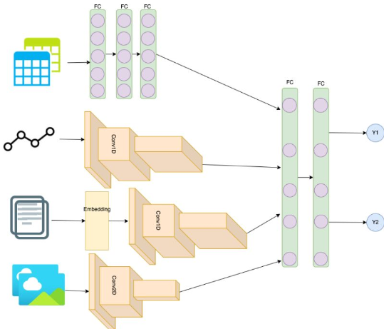
Deep Learning requires much more of an ARCHITECT mind set than traditional Machine Learning. In a sense, the feature engineering work has been moved to the design of very specialized computational blocks in DL using smaller units (LSTM, Convolutional, embedding, Fully connected, …). I always advise to start with a simple net when architecting a model such that you can build your intuition. Jumping right away into a Transformer model may not be the best way to start.
DL is very powerful in the case of multi-modal input data: time series, tabular data, text data, image data. One approach is to encode all those different data types into a simple vector and feed that into a logistic regression (LogReg) or a linear regression (LR) (or with more fully connected layers to add non-linearity) depending on if you need to perform classification or regression. When developing a simple model, start with a low capacity network and increase little by little the complexity to reduce the bias while adding regularization to keep the variance low.
A conv layer is meant to learn local correlations. Multiple successive blocks of conv and pooling layers allows to learn the correlations at multiple scales and they can be used on image data (conv2d), text data (text is just a time series of categorical variables) or time series (conv1d). For example you can encode an image using a series of conv2d and pooling layers like in VGG (https://lnkd.in/g6Jp6NmD, https://lnkd.in/gDjUGWFE). You can encode text data using an embedding (pretrained obviously https://lnkd.in/gt5N-i6R) followed by a couple of conv1d layers. And you can encode a time series using series of conv1d and pooling layers.
I advise against using LSTM layers when possible. The iterative computation doesn’t allow for good parallelism leading to very slow training (even with the Cuda LSTM). For text and time series ConvNet are much faster to train as they make use the of the matrix computation parallelism and tend to perform on par with LSTM networks (https://lnkd.in/g-6Z6qCN). One reason transformers became the leading block unit for text learning tasks, is its superior parallelism capability compared to LSTM allowing for realistically much bigger training data sets.
In general it is not too hard to train on multi-modal data. As a simple example:
- time series vector = Pool1d(Conv1d(Pool1d(Conv1d(time series))
- image vector vector = Pool2d(Conv2d(Pool2d(Conv2d(image data))
- text vector = Pool1d(Conv1d(Pool1d(Conv1d(Embedding(text data)))
- tabular data vector = FC(FC(tabular data)) => X = FC(FC(time series vector, tabular data vector, text vector, image vector)) The nice thing with DL, you can train on multiple targets at once using multiple target heads: Y_1 ~ LR(X), Y_2 ~ LogReg(X)
Recommender Engine
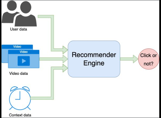
Netflix matrix factorization Recsys paper A multi-task framework for metric learning with common subspace Linkedin linkedy DGCN: Diversified Recommendation with Graph Convolutional Networks recsys
Recommender Engine might be one of the most PROFITABLE Machine Learning Model paradigms right now but I think it doesn’t get the recognition it deserves! There are many ways to generate money with ML but the niche business applications where Rec Engines are typically used makes it a more certain high ROI ML application in general. The business value of Rec engines is clear: personalized matching between a user and a product. That is the bread and butter of many big tech companies:
- search engine: Google search, Amazon Product Search, …
- Ads ranking: Google and Meta generate 65% of the world digital ad revenue
- Feed ranking: FB, Instagram, LinkedIn, …
-
Product Recommendation: Netflix’s landing page, …
-
The modern approach to Rec Engine can be tracked back to the 2006 Netflix Recommendation contest (https://lnkd.in/ds6WWEG3) where the Latent Matrix Factorization method won second place (https://lnkd.in/dz4q7Xnx). Surprise is a nice python implementation: http://surpriselib.com/. In a supervised learning term, we use user data, product data and context data as input to estimate the affinity of a user to a product: affinity ~ F(user data, product data, context data). Those algorithms are peculiar because we want to use the same user and product population at training time than inference time: in a sense, we want to overfit on the user behavior.
- Now Deep Learning dominates the field by extending on the original linear models and it led to many new NN architectures. Embeddings provide a natural mechanism to featurize the large users and products spaces and their related behavior history. Some architecture examples:
- Multi gate Mixture of Experts for Youtube videos recommendation: https://lnkd.in/dE6XZvJx
- Multi-Task Metric Learning for multi-staged inference when the product space is too large: https://lnkd.in/dSpiR9GA, https://lnkd.in/dZErXbpE
- Two Tower models for retrieval: https://lnkd.in/dh3Xtmyc
- Multi-tower model for ads ranking in Pinterest: https://lnkd.in/d_uPNSAH
- Diversified recommendation with Graph Convolutional Networks: https://lnkd.in/dfcVYeDJ
-
Autoencoder-based recommender: https://lnkd.in/dET64Pvs
- This is an interesting space and a valuable expertise to have those days. I wish there were more textbooks on the subject! One to get started: https://lnkd.in/deMyYw5e
How to detect Data Drift
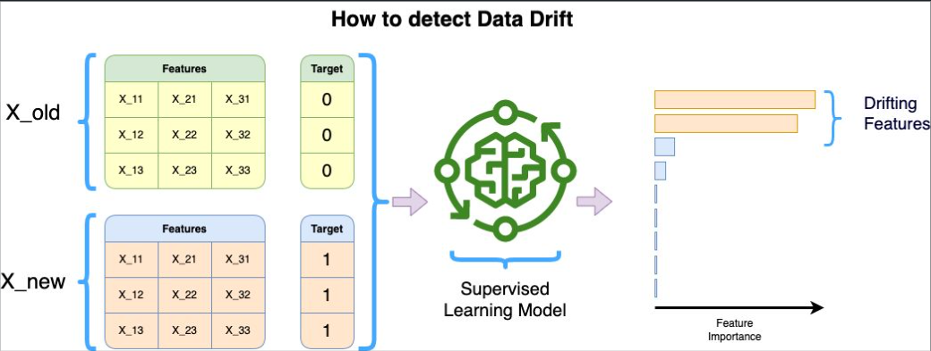
- There is one simple technique I like to use to detect DATA DRIFT for Machine Learning applications. First, take a current data set and let’s call it X_now. Then let’s take an old data set and let’s call it X_old. You could imagine having different X_old for different time scales: 1 week ago, 1 month ago, 1 year ago, … Let’s now create an artificial target Y_now where all the values are 1 and another Y_old where all the values are 0. Y_old would be paired with the X_old samples and Y_now with the X_now ones. We can concatenate X_now with X_old and Y_now with Y_old:
X = [X_now, X_old]
Y = [Y_now, Y_old]
Now take that data (X,Y) and train a Supervised Learning algorithm that has a good built-in Feature Importance measurement process. For example, I like to take a Random Forest algorithm that has typically a Feature Importance measured as a mean entropy or Gini gain per split through the whole forest. If one or few features are coming out as having a high feature importance to predict that artificial target, this is a strong evidence that those features have been drifting over time!
What techniques do you like to use to detect Data Drift?
One common technique to detect data drift in machine learning applications is to compare the statistical properties of different data distributions over time. Here are a few techniques commonly used to detect data drift:
-
Monitoring Descriptive Statistics: Track key descriptive statistics, such as mean, standard deviation, or skewness, for relevant features in the dataset. Any significant changes in these statistics over time can indicate data drift.
-
Statistical Hypothesis Testing: Apply statistical tests to compare the distributions of different datasets. For example, you can use the Kolmogorov-Smirnov test, the Anderson-Darling test, or the Mann-Whitney U test to check if the data distributions are significantly different.
-
Drift Detection Methods: There are specific drift detection methods designed to identify changes in data distributions. Examples include the Drift Detection Method (DDM), the Page-Hinkley Test, the Sequential Probability Ratio Test (SPRT), and the Cumulative Sum (CUSUM) algorithm. These methods analyze incoming data incrementally and raise an alarm when a significant change is detected.
-
Machine Learning Model Monitoring: Track the performance of your machine learning models over time. Monitor metrics such as accuracy, precision, recall, or the area under the ROC curve (AUC-ROC). A significant drop in performance can indicate a drift in the data.
-
Feature Importance Analysis: Use feature importance techniques to assess which features have the most impact on model predictions. If the importance of certain features changes significantly over time, it suggests that those features may be drifting.
-
Domain Expert Knowledge: Incorporate domain expertise to identify potential sources of data drift. Experts can provide insights into changes in the data-generating process, external factors impacting the data, or shifts in user behavior that might affect the data distribution.
- It’s important to note that data drift detection is an ongoing process, and there is no one-size-fits-all solution. Different techniques may be more suitable depending on the specific problem, the nature of the data, and the available resources. Combining multiple methods and continuously monitoring the data can help you identify and address data drift in machine learning applications.
- The technique described in the provided explanation is one way to detect data drift by leveraging supervised learning algorithms and feature importance analysis. The reasoning behind setting Y_old (target for old data) to all 0 and Y_now (target for current data) to all 1 is to create an artificial target variable that represents a binary classification problem. This allows us to train a supervised learning algorithm to predict whether a data sample belongs to the old or new dataset.
- By concatenating X_old with X_now and Y_old with Y_now, we create a combined dataset (X, Y) where the algorithm can learn to differentiate between the old and new data samples. The intention is to analyze the feature importance provided by the trained model. If specific features are assigned high importance in predicting the artificial target (i.e., distinguishing between old and new data), it suggests that those features have changed or drifted over time.
- Data drift refers to changes in the underlying data distribution over time, which can impact the performance and reliability of machine learning models. By training a model to distinguish between old and new data and examining the feature importance, we can identify which features contribute significantly to discriminating between the datasets. If the importance of certain features is high, it indicates that those features have undergone substantial changes or drift, potentially influencing the model’s performance when applied to new data.
- In summary, by training a model to discriminate between old and new data and analyzing the feature importance, this technique aims to identify features that have changed over time, serving as an indicator of data drift. It provides insights into which features contribute most to the distinction between datasets and highlights potential shifts or inconsistencies in the data that might affect model performance.
Kolmogorov-Smirnov test
- The Kolmogorov-Smirnov test, often abbreviated as the K-S test, is a nonparametric test used in statistics to determine whether two underlying one-dimensional probability distributions differ, or to compare a sample with a reference probability distribution. It is widely used for comparing two empirical distributions or an empirical distribution against a theoretical one.
- The test is based on the maximum distance between these distributions, specifically focusing on their cumulative distribution functions (CDFs). Here’s a brief overview of how it works:
- Null Hypothesis (H0): The null hypothesis states that there is no difference between the two distributions being compared.
- Test Statistic: The K-S test calculates the maximum difference (D) between the two cumulative distribution functions. For two empirical distributions, this is typically visualized as the greatest vertical distance between the two CDFs.
- Critical Value and P-Value: Based on the test statistic and the sample size, a p-value is calculated. This p-value indicates the probability of observing such a difference if the null hypothesis were true. If the p-value is less than a chosen significance level (commonly 0.05), the null hypothesis is rejected, suggesting a significant difference between the distributions.
- Two-Sample vs One-Sample Test: The K-S test can be applied in two forms: the one-sample K-S test compares a sample with a reference probability distribution, and the two-sample K-S test compares two empirical distributions.
- Advantages and Limitations: The test is nonparametric, requiring no assumption about the distribution of data, making it versatile. However, it is less powerful than some parametric tests when their assumptions are met, and it might not be suitable for discrete distributions or small sample sizes.
- The K-S test is widely used in various fields such as finance, environmental science, and engineering, where understanding the distribution of data is crucial.
Prevent data drift
- Designing machine learning infrastructure systems to systematically prevent or at least detect data drift is crucial for maintaining the accuracy and reliability of ML models over time. Data drift refers to the change in the model’s input data distribution over time, which can degrade the model’s performance. Here’s how you can design ML infrastructure to address this challenge:
1. Data Monitoring
- Implement Continuous Data Monitoring: Set up systems to continuously monitor data quality and characteristics. This includes tracking changes in data distributions, outliers, and missing values.
- Automated Alerts: Develop automated alerting mechanisms that notify relevant teams when significant data drift is detected.
2. Versioning and Data Lineage
- Data Versioning: Implement data versioning to track changes over time. This helps in identifying when and how the data has changed.
- Maintain Data Lineage: Keeping records of data lineage allows teams to trace back through the data pipeline to identify sources of drift.
3. Periodic Model Evaluation
- Regular Model Performance Checks: Schedule regular evaluations of the model against current data to check for performance degradation.
- Benchmarking Against Fresh Data: Regularly test the model with new, unseen data to ensure it still performs well under current conditions.
4. Robust Data Pipeline
- Build Robust Data Pipelines: Ensure that the data pipeline is robust against common issues like missing data, format changes, or pipeline failures.
- Automated Data Quality Checks: Incorporate automated checks for data quality at various points in the pipeline.
5. Adaptive Model Training
- Incremental Learning: Implement models capable of incremental learning, where they can adapt to new data patterns over time.
- Automated Retraining Pipelines: Set up automated pipelines for retraining models with new data.
6. Feedback Loops
- Incorporate User Feedback: Establish mechanisms for incorporating user feedback into the model training process.
- Post-Deployment Monitoring: Continuously monitor the model’s performance in the production environment and use this feedback for improvements.
7. Experimentation and A/B Testing
- A/B Testing: Conduct A/B tests to compare the performance of models under different data scenarios.
- Experimentation Framework: Develop a robust experimentation framework to test models under various conditions.
8. Documentation and Governance
- Maintain Comprehensive Documentation: Keep detailed documentation of models, data sources, and changes over time.
- Data Governance: Establish strong data governance policies to maintain data quality and integrity.
9. Collaborative Approach
- Cross-Functional Teams: Encourage collaboration between data scientists, engineers, and domain experts to better understand and mitigate data drift.
- Training and Awareness: Provide training and awareness programs for team members to recognize and address data drift.
10. Use of Advanced Tools and Technologies
- Leverage Advanced Monitoring Tools: Use advanced tools that can detect data drift using statistical methods and machine learning techniques.
-
Scalable Infrastructure: Ensure that the infrastructure is scalable to handle increasing data volumes and complexity.
- By combining these strategies, ML infrastructure can be designed to not only detect but also prevent data drift, ensuring that models remain effective and reliable over time.
Explain reasoning behind offline and online gap in ML system evaluation and mitigation strategies?
- The gap between offline and online evaluation in machine learning (ML) systems can significantly impact the performance and reliability of these systems in real-world applications. This gap is primarily due to differences in the environments and data used for training and testing these systems. Here are the main reasons behind this gap and some strategies to mitigate it:
Reasons Behind the Gap
-
Data Distribution Differences: Offline evaluations often use historical data, which might not represent current or future conditions. Online evaluations, in contrast, deal with real-time data that may include new patterns not present in the training set.
-
Feedback Loop: Online systems often have a feedback loop where the system’s outputs can influence future inputs (e.g., user interactions). This dynamic is usually absent in offline evaluations.
-
Scale and Complexity: The complexity and scale of real-world data can be much higher than the data used in offline settings. Online systems may encounter more varied and unpredictable scenarios.
-
User Behavior: User interactions and behavior can significantly differ from what is modeled or anticipated during offline evaluations. Users may react to the system’s outputs in unforeseen ways.
-
Latency and Performance Constraints: Online systems need to adhere to stricter performance and latency requirements, which might not be fully simulated or considered in offline tests.
Mitigation Strategies
-
Continuous Monitoring and A/B Testing: Implementing A/B testing and continuous monitoring in the live environment helps in understanding how the model performs in real-world scenarios and adjusting it accordingly.
-
Data Recency and Relevance: Ensuring the data used for offline evaluation is recent and relevant can help reduce the gap. This includes updating the datasets regularly to reflect current trends and patterns.
-
Simulating Online Conditions: Enhancing offline evaluation by simulating online conditions as closely as possible, including user behaviors, feedback loops, and real-world constraints.
-
Model Updating and Re-training: Regularly updating and re-training the model with new data collected from the online environment can help the model adapt to changing patterns and behaviors.
-
User-Centered Testing: Incorporating user studies or testing that involves actual user interactions can provide insights that purely data-driven offline tests might miss.
-
Hybrid Approaches: Combining both offline and online evaluation methods to balance the strengths and weaknesses of each approach.
-
Feature Flags and Canary Releases: Gradually rolling out new models or features to a small subset of users before a full deployment can help in identifying issues early.
-
Robustness and Stress Testing: Conducting robustness and stress testing under various simulated conditions can prepare the system for unexpected scenarios.
- By applying these strategies, the gap between offline and online evaluation can be narrowed, leading to more reliable and effective machine learning systems in real-world applications.
How do wide and deep models handle feature crossing in recommender systems?
How to decompose Bias and Variance from the Data
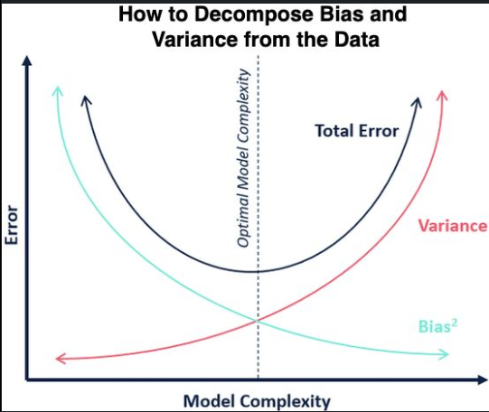
Have you ever tried to compute the BIAS and VARIANCE separately from the data? It is not as simple as one may think! I think we all know the typical decomposition formula (https://lnkd.in/gjQ3n7fj):
E[(y - f(x))^2] = Bias[f]^2 + Var[f] + sigma^2 with Bias[f] = E[f(x)] - f(x)
But did you realize that the Expected value and Variance range over different realizations of the training data D = (X, Y) sampled from the same probability distribution P(X,Y)? To obtain the Mean Square Error (MSE) you need then to run an expected value over the instance distribution this time
MSE = E_x[E[(y - f(x))^2]]
Estimating E_x[.] is easy, you just need to run a sum over the test set: sum(.) / N, where N is the number of samples in the test set. But how do you go about the first expectation?
One way I find intuitive to understand (https://lnkd.in/g49Q9Tjr) is to create M bootstrap samples of the training data D and to train your learner L on each of those sample. For each instance of the test set you can then predict M different values for each of the trained learners. And then you can estimate the expected value for each instance as
mean = sum_i [ f(x_i) ]/ M variance = sum_i [ (f(x_i) - mean)^2 ]/ (M - 1)
And easily estimate the local Bias and Variance for each instance and then average over all the instances in the test set to get MSE.
The following article compares 3 different methods to estimate the Bias and Variance decomposition on real data: https://lnkd.in/gptRH8gp
Is that something you have been wondering about?
Feature Selection Method
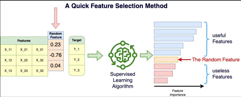
This is a technique I like to perform a quick FEATURE SELECTION for Machine Learning applications. I tend to call it the “Random Bar” method! Let’s assume you have a feature set X and a target Y. Let’s create a random vector V (for example np.random.normal(size=(1, 100))) and append that vector as a new feature to X:
X’ = [X, V]
X’ is just the original feature set with additionally the new random feature. Keep in mind that this new feature cannot possibly help to predict the target Y since it is random! Now, take that data (X’, Y) and train a Supervised Learning algorithm with a Feature Importance measure that is relevant for you application. Intuitively, the mean entropy gain per split of tree based algorithms (Random Forest, Xgboost, …) is a convincing measure of feature importance to me. The statistical fluctuation of the data is such that even the random feature will be attributed a non-zero feature importance by the algorithm, but we know it is artificial. Any feature with a lower feature importance than the random feature has to be useless to predict the target and the features with a higher feature importance are at least better than random noise at predicting the target.
This is especially useful if you have thousands of features and you want to weed out quickly the ones that won’t have any impact in the learning process. This is also a method that can be used for highly non-linear data as opposed to LASSO (for example) that tends to only understand linear relationships in the data. The random feature is a “Random Bar” because this is the minimum bar a feature needs to beat to be a part of the potentially useful features set. Now it doesn’t mean there are not additional features that could be beneficial to further remove to optimize your model. Do you know if this method has a more jargon-y name?
For typical recommendation system, a common practice is to continuously train the model. Suppose that we launched a 6 model ago and we have continuously trained it. Consider that if we trained a month starting off with the 6 month ago checkpoint and trained with 3 months of fresh data. How do we use the production model to make the new model with 3 months of data better?
- Here are a few ways to leverage the production model to improve a new model trained on more recent data:
- Use the production model as a starting point - initialize the new model with the weights from the production model rather than random initialization. This allows the new model to benefit from what was already learned.
- Employ distillation - use the predictions from the production model as soft targets to regularize the training of the new model. This helps transfer knowledge from the production model.
- Combine outputs - average or ensemble the predictions from both models. The production model provides a historical viewpoint while the new model incorporates latest trends.
- Focus new model training on weaknesses - use the production model to find examples the new model gets wrong. Focus sampling and regularization techniques on those cases during training.
- Update production model incrementally - periodically update the production model with new data rather than training a separate model. This allows continuous integration of new data to an already robust model.
- The key is leveraging the existing production model as an additional source of knowledge and regularization for training improved models, rather than training each new model from scratch. The production model encapsulates previously learned patterns.
How are ID features handled in LLM recommender models?
- Here are some common ways ID features are handled in large language model (LLM) based recommender systems:
- Hash Encoding - ID features like user_id or item_id are hashed to an embedding space. This embedding can be concatenated to the other feature embeddings and input to the LLM.
- Learned Embedding - The model learns an embedding lookup table for ID features. The ID embeddings are concatenated with other features as input to the LLM.
- Entity Embeddings - ID features are treated as entities. The model leverages a pre-trained entity embedding table like from knowledge bases.
- Contextualization - The ID features are converted to natural text descriptions. For example, user_id=1525 -> “User is a 28 year old male from New York City”. This text is concatenated to input.
- Metadata Enrichment - ID features are used to retrieve associated meta data like user profiles or item attributes. This metadata is encoded as text and provided as additional context to the LLM.
- Cross-Attention - Self-attention layers in the LLM can use ID embeddings as an additional “memory” for the model to cross-attend to. This allows modeling interactions between IDs.
- Personalization Layers - Dedicated personalization or ranking layers after the base LLM can take ID embeddings as input for personalized ranking.
- The overall goal is to represent IDs in a way that the model can effectively incorporate them into reasoning about user-item interactions and preferences. Hashing, embeddings and text contextualization are common techniques for encoding ID features into the LLM input.
Self Instruct aligning language models with self generated instructions
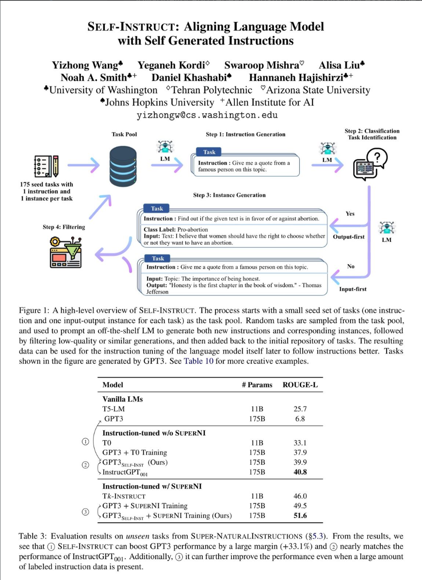
Sergio Valmorisco Sierra Sergio Valmorisco Sierra • 2nd Global Senior Data Scientist at JLL 3h • 3 hours ago
Follow
Large “instruction-tuned” language models (finetuned to respond to instructions) have demonstrated a remarkable ability to generalize zero-shot to new tasks. Nevertheless, they depend heavily on human-written instruction data that is limited in quantity, diversity, and creativity, therefore hindering the generality of the tuned model. In this work, the authors introduce SELF-INSTRUCT, a semi-automated process for instruction-tuning a pretrained LM using instructional signals from the model itself.
The overall process is an iterative bootstrapping algorithm, which starts off with a limited (175 in their study) seed set of manually-written instructions that are used to guide the overall generation. In the first phase, the model is prompted to generate more broad-coverage instructions that define (often new) tasks. Given the newly-generated set of instructions, the framework also creates input-output instances for them, which can be later used for supervising the instruction tuning. Finally, various measures are used to prune low-quality and repeated instructions. This process can be repeated for many interactions until reaching a large number of tasks.
Applying their method to vanilla GPT-3, the authors demonstrate a 33% absolute improvement over the original model on the SUPER-NATURALINSTRUCTIONS dataset, on par with the performance of InstructGPT001, which is trained with private user data and human annotations. For further evaluation, they curate a set of expert-written instructions for novel tasks, and show through human evaluation that tuning GPT-3 with SELF-INSTRUCT outperforms using existing public instruction datasets by a large margin, leaving only a 5% absolute gap behind InstructGPT001.
Code and data: https://lnkd.in/d_Wd52Uu Paper: https://lnkd.in/dS8wuBBh
How do you handle hashing for a large billion-scale ID cardinality?
- Here are some techniques to handle hashing large cardinality ID features in billion-scale datasets:
-
Use a 64-bit or 128-bit hash function: MD5, SHA-1, SHA-256 etc. The large output space can accommodate billions of IDs with low collision probability.
-
Use multiple hash functions and concatenate the hashes. For example, take MD5 + SHA-1 hashes to get a 128 bit hash. This further reduces collisions.
-
Use locality sensitive hashing (LSH) to map similar IDs to same buckets with high probability. Makes model learning efficient.
-
Use modulo N hashing to bucket IDs into N buckets. Choose N smartly to distribute IDs while fitting in memory.
-
Maintain an LRU cache of recent/frequent IDs for quick lookup. Assign hash on first occurrence. Handles skewed distributions.
-
Use consistent hash functions so hashes don’t change as data scales. For example, farmhash, xxhash.
-
Store hashes in sparse matrix format with IDs as keys for memory efficiency.
-
Preprocess to assign hashes and save mapping to disk. Load portions during training as needed.
-
Learn multiple hash tables with different hash functions. Adaptively pick hash to balance load.
- The key principles are using long hash outputs, multiple hash functions, bucketing techniques, caching for skewed data, and intelligent memory/disk management to make billion-scale ID hashing feasible.
What kind of feature crossing techniques in recommender systems?
-
Polynomial Features - Create new features by taking all polynomial combinations of original features like user_id x item_id, user_id x time etc.
-
Feature Hashing - Hash the concatenated values of features to generate cross features like hash(user_id + item_category).
-
Embeddings - Learn joint embeddings for feature combinations like user_id + item_id. Useful for high cardinality categorical features.
-
Multi-way Interactions - Explicitly model high-order interactions between multiple features using tensor/factorization machines, deep crossing networks etc.
-
Knowledge Graphs - Model relationships between different features via knowledge graph connections. Allows feature crossing via graph traversals.
-
Neural Networks - Deep neural nets with cross-layer connections can learn implicit feature crosses and interactions.
-
Automatic Crossing - Use feature transformation techniques like FTRL to automatically construct and select useful crosses.
-
Domain-driven Crossing - Combine features informed by domain knowledge like user_geo x item_category for location-based personalization.
-
The goal is to effectively capture the interactions between different features to create better recommendation models. Techniques range from manual crosses to learned models like deep nets that implicitly cross features through non-linear transformations and hidden layers.
ANN and it’s selection criteria
Approximate Nearest Neighbor (ANN) algorithms are essential in machine learning for efficiently finding close neighbors to a query point in high-dimensional spaces. Unlike exact nearest neighbor searches, which can be computationally expensive and slow, ANNs trade off a bit of accuracy for significant gains in speed and memory efficiency. This is particularly useful in large-scale applications like recommender systems, computer vision, and high-dimensional data clustering. Here’s an overview of ANN and the selection criteria for these algorithms:
Approximate Nearest Neighbors (ANN)
Key Concepts
- Speed vs. Accuracy Trade-off: ANN algorithms prioritize speed and computational efficiency over exact accuracy in finding the nearest neighbors.
- High-Dimensional Spaces: They are particularly useful in high-dimensional spaces where the curse of dimensionality makes exact nearest neighbor searches impractical.
Common Algorithms
- Locality-Sensitive Hashing (LSH): Uses hashing to bucket points such that the probability of collision is higher for points which are close to each other.
- KD-trees and Ball Trees (for Moderate Dimensions): Effective in lower to moderate dimensional spaces.
- Hierarchical Navigable Small World (HNSW): Gains popularity for its balance between search efficiency and accuracy.
- Product Quantization: Divides the space into a Cartesian product of low-dimensional subspaces and quantizes each subspace separately.
- Tree-based Methods (like Annoy): Build tree structures to partition the space and efficiently traverse these trees to find nearest neighbors.
- Graph-based Methods: Create graphs where nodes represent data points, and edges connect each point to its nearest neighbors.
Selection Criteria for ANN Algorithms
1. Dimensionality of Data
- High vs. Low Dimensions: Some algorithms perform better in lower-dimensional spaces (e.g., KD-trees) while others are tailored for high-dimensional data (e.g., LSH, HNSW).
2. Dataset Size
- Large Datasets: For very large datasets, consider memory-efficient algorithms like HNSW or product quantization.
- Small to Medium Datasets: Tree-based methods like Annoy or Ball Trees might be sufficient.
3. Query Speed
- Latency Requirements: If low latency is crucial, prioritize algorithms known for their high-speed querying, like HNSW or Annoy.
4. Accuracy Requirements
- Precision-Recall Trade-off: Some applications might tolerate a lower recall for a significant gain in speed, while others might need higher precision.
5. Update Frequency
- Dynamic vs. Static Datasets: If the dataset changes frequently (insertions/deletions), consider whether the algorithm supports dynamic updates efficiently.
6. Memory Usage
- Hardware Constraints: Evaluate the memory footprint of the algorithm, especially important in resource-constrained environments.
7. Ease of Implementation and Maintenance
- Complexity: Consider the complexity of implementing and maintaining the algorithm, including the availability of libraries and support.
8. Scalability
- Scaling with Data Size: Ensure the algorithm scales well with the increase in data size, both in terms of memory and computational efficiency.
9. Parallelism and Distribution
- Support for Parallel Processing: For large-scale applications, consider if the algorithm can leverage multi-core processors or distributed computing environments.
Conclusion
The choice of an ANN algorithm depends on a delicate balance of these factors, tailored to the specific needs and constraints of your application. It’s often beneficial to conduct empirical tests with a subset of your data to determine which algorithm provides the best trade-off between speed, accuracy, and resource consumption for your particular use case.
How do we handle categorical features in recommender systems?
-
Handling categorical features in recommender systems is a key aspect of the model building process, as these systems often deal with a large amount of categorical data, such as user IDs, item IDs, genres, locations, etc. The way these features are processed and integrated into the model can significantly impact the system’s performance. Here are some common strategies for handling categorical features in recommender systems:
-
Encoding - Convert categories to numeric ids or one-hot vectors. Common encodings are label encoding, one-hot encoding, mean encoding, etc.
-
Embeddings - Map categories to low dimensional dense vector embeddings. Learned jointly with model. Captures semantic meaning.
-
Hashing - Hash categories to numeric buckets to handle high cardinality. Useful when number of categories is large.
-
Clustering - Group infrequent categories into clusters. Reduces sparsity.
-
Count Features - Derive useful count statistics for each category like frequency, co-occurrence counts etc.
-
Smoothing - Apply smoothing techniques like adding small constant to infrequent categories to reduce sparsity.
-
Grouping - Manually group related categories into higher level categories based on domain knowledge. Reduces cardinality.
-
Segmentation - Divide users/items into segments based on categories for segment-specific modeling.
-
Decision Trees - Use tree-based models like XGBoost that can handle categorical splits.
-
Regularization - Use regularization when training models to avoid overfitting sparse categories.
-
The main goals are reducing sparsity, encoding semantics, and handling high cardinality. This allows the model to effectively leverage categorical information for making better recommendations.
-
Association retrieval is a method proposed by, “Solving the Sparsity Problem in Recommender Systems Using Association Retrieval” , which involves exploring transitive associations between users based on their feedback data. This method aims to alleviate the sparsity problem and improve recommendation quality.
Is there any downside to Feature Hashing (Hashing Trick)?
- Feature Hashing, also known as the hashing trick, is a technique used in machine learning to efficiently encode high-dimensional categorical data into a lower-dimensional space. While it offers several advantages, particularly in terms of memory efficiency and scalability, there are some downsides to be aware of:
1. Collision Risk
- Hash Collisions: Since the hashing trick maps a potentially large number of features to a smaller number of dimensions, different original features can end up with the same hash value. This is known as a collision.
- Information Loss: Collisions can lead to information loss, as the model cannot distinguish between features that have been hashed to the same value.
2. Irreversibility
- Loss of Original Values: Once features are hashed, it’s not possible to reconstruct the original values. This can be a significant downside when interpretability or further analysis of original features is needed.
3. Tuning Hash Space Size
- Determining Dimensions: Choosing the appropriate size for the hash space is a trade-off. A smaller size leads to more collisions (and potential loss of information), while a larger size reduces collisions but increases memory and computational requirements.
- No Optimal Rule: There’s no definitive rule for the best size, and it often requires experimentation and domain knowledge.
4. Lack of Weighting Distinction
- Equal Weighting: The hashing trick does not differentiate between features in terms of their importance or frequency. Each feature is hashed independently of its significance.
5. Difficulty in Handling New Features
- Dynamic Feature Set: In scenarios where new features are continuously added, managing the hash function and ensuring consistent hashing for new and old features can be challenging.
6. Potential for Overfitting
- Sparse Features: If the hashed feature space is still relatively high-dimensional and sparse, it can lead to overfitting, especially with models sensitive to high-dimensional spaces.
7. No Native Support for Feature Interactions
- Feature Crosses: The hashing trick doesn’t natively handle feature interactions. Additional steps or models are required to capture interactions between features.
8. Model Dependency
- Algorithm Suitability: The effectiveness of feature hashing can depend on the type of model being used. Some models may work better with hashed features than others.
Conclusion
- Feature Hashing is a powerful tool, especially for handling large-scale and high-dimensional data. However, its suitability depends on the specific requirements and constraints of the machine learning task at hand. The downsides, particularly regarding collisions, irreversibility, and the tuning of hash space size, need to be carefully considered and managed.
How do wide and deep models handle feature crossing in recommender systems ?
- In recommender systems, handling feature interactions, including feature crossing, is crucial for making accurate predictions. “Wide and deep” models, a concept popularized by a research paper from Google, are particularly effective in this regard. Here’s a breakdown of how these models handle feature crossing:
- Wide Component:
- The “wide” part of a wide and deep model is a linear model (like logistic regression).
- It is particularly good at handling explicit feature interactions (feature crossing).
- These interactions are usually hand-engineered and can be based on domain knowledge. For instance, in a movie recommendation system, a crossed feature could be the combination of “user’s age group” and “movie genre”.
- The wide component helps in memorizing specific feature combinations that are useful for the prediction.
- Deep Component:
- The “deep” part is a feed-forward neural network.
- It is capable of learning high-level, abstract representations of data through its hidden layers.
- In the context of feature interactions, the deep network automatically learns implicit feature interactions. As data passes through the layers, the network combines features in various ways, essentially learning which combinations of features (even if not explicitly defined) are meaningful for predictions.
- This part is more about generalization rather than memorization, which complements the wide part.
- Combination of Wide and Deep:
- The key to the wide and deep model is in combining these two approaches.
- While the wide part handles specific, known interactions and memorization of particular feature combinations, the deep part discovers and generalizes the unknown, implicit interactions.
- By combining these, the model can leverage the strengths of both linear and nonlinear approaches.
- The outputs of both the wide and deep components are combined (usually through a sum operation) to make the final prediction.
- Application in Recommender Systems:
- In recommender systems, this approach allows the model to capture specific rules and patterns through the wide component (like “users of a certain demographic tend to like certain types of movies”) while also adapting to complex and subtle user preferences and behaviors via the deep component.
- This results in a more robust and accurate system, capable of handling a wide range of recommendation scenarios.
-
Wide component: The wide linear component explicitly models feature crosses and interactions through techniques like polynomial expansion, embedding crosses, product transformations etc. This memorizes certain cross-features.
-
Deep component: The hidden layers of the deep neural network component automatically learn latent crosses and interactions between features through non-linear transformations and dense embeddings.
-
Shared embedding layer: Having a shared wide-deep embedding layer allows embeddings to represent both singleton features and interactions for the wide and deep parts respectively.
-
Wide input to deep: The wide model component’s crossed features can be provided as additional input to the deep component after the embedding layer to inform the deep model.
-
Deep output to wide: The hidden layers of the deep component can generate new interaction features to expand the input to the wide component.
-
Ensembling: The wide and deep components capture different types of crosses which can then be ensembled or concatenated into final predictions.
- Joint training: End-to-end joint training allows the wide, deep and shared components to handle crosses in a coordinated manner.
- The wide component memorizes cross-features while the deep component generalizes feature interactions. Combining them allows leveraging both memorization and generalization to improve recommendation performance.
Deep and Cross
-
Deep & Cross Network (DCN) is a neural network-based model that effectively combines “Deep” neural network learning and “Cross” feature interactions for recommender systems. Here is how it handles feature crossing:
-
Explicit Feature Crosses: DCN introduces explicit cross layers that take element-wise product between feature embeddings to model interactions. For example, Cross(Embedding(user), Embedding(item))
-
Cross Network: The cross layers are stacked to learn higher-order interactions like Cross(Cross(A,B), C). This cross network is capable of memorizing and generalizing feature crosses.
-
Deep Layers: The standard deep neural network layers learn implicit feature crosses through non-linear transformations and latent interactions.
-
Cross-stitch Units: These units combine the implicit crosses from deep layers and explicit crosses from cross-layers, enabling them to work together.
-
Residual Learning: The input embeddings are added to later cross-layers using residual connections. This allows better gradient flow during training.
-
Joint Training: The entire network comprising deep layers, cross layers and cross-stitch units is trained end-to-end, allowing an integrated model of crosses.
-
In summary, DCN introduces specialized cross-layers to model explicit crosses, which are then combined with deep neural network layers to get both explicit and implicit crosses in an integrated model. The joint training and architecture allows effective learning of crossed features.
What does feature crossing mean? how do you handle high cardinality in data when crossing?
- Feature crossing refers to combining multiple features into a new feature to capture interactions between them. This allows machine learning models to better learn non-linear relationships from the data.
- Feature crossing, also known as feature interaction, is a technique in machine learning where you create new features by crossing (or combining) two or more existing features. The idea is to capture interactions between different features that might be predictive but are not captured when considering the features independently. For example, in a real estate model, crossing “city” and “property type” might reveal patterns specific to apartments in urban areas that wouldn’t be apparent when looking at either feature alone.
- Handling high cardinality in data, especially when performing feature crossing, can be challenging due to the exponential increase in the number of unique feature combinations. High cardinality means a feature has a large number of unique values. Here are some strategies to manage this:
- Some ways to handle high cardinality features for crossing:
- Feature Hashing: Hash the high cardinality features into buckets first before crossing to reduce dimensionality.
- Modular Hashing: Take a modulo of the feature values with some prime number to put them in smaller buckets.
- Embedding Crossing: Learn low-dimensional embeddings for high cardinality features and then cross the embeddings.
- Sampling: Randomly sample from the long tail of infrequent feature values when crossing.
- Frequency-based Crossing: Only cross features that co-occur above a certain frequency threshold.
- Cross Feature Selection: Use regularization or feature selection to determine most useful cross features.
- Two-stage Crossing: First independently embed high cardinality features, then cross the embeddings.
- Locality Sensitive Hashing: Map similar feature values to same buckets before crossing.
- The main idea is to first reduce the cardinality of individual features, then cross the lower-dimensional representations. This allows feasible and useful crossing of high cardinality categorical features like user_ids or item_tags.
For a recommender system’s training data, say we have 100M data samples, 5000 for retrieval, 5 for ranking. For the ranking stage, we want to log features. How best do we log for features since the ones that didn’t get to ranking could also be relevant?
-
Here are a few ideas for how to handle logging of features for a multi-stage recommender system with a large training dataset but small set available for the ranking stage:
-
Cache features from full dataset - Precompute and cache feature transformations like log counts, embeddings etc. for the full dataset. Then lookup for small set.
-
Sample more for ranking - Increase the sample size taken for final ranking stage to better cover full distribution.
-
Reweight by inverse propensity - Assign higher importance weights to less frequent features sampled for ranking.
-
Two-stage model - Train a lightweight model on full data for feature generation, then train ranking model on sample.
-
Learn feature distribution - Model the distribution of features in full dataset. Sample from distribution for ranking set.
-
Hybrid online/offline - Use offline large-scale model to generate candidate features, finetune online with features from ranking sample.
-
Imputation - For missing values in ranking set, impute intelligently using statistics from full data.
-
Generative model features - Use generative models like GANs trained on full data to generate synthetic features for tail items.
-
The key is to leverage the full dataset as much as possible for feature engineering and importance weighting, while dealing with the computational constraints of having a small ranking set. Hybrid online/offline approaches can work well in this case.
-
In a recommender system, especially one using a two-stage approach with retrieval and ranking stages, feature logging is crucial for understanding and improving the model’s performance. The challenge in your scenario lies in effectively logging features for both the small subset of items that reach the ranking stage and those that do not but might still hold relevance. Here are strategies to approach this:
- Log Features at Both Stages:
- Log features for all items at the retrieval stage, not just the 5000 that make it to ranking. This can provide insights into why certain items were selected for ranking and others were not.
- For the ranking stage, log detailed features for the final 5 items. This information is crucial for understanding the final decision-making process of the model.
- Sampling Strategy:
- Given the large dataset (100M samples), consider a sampling strategy for logging. Randomly select a representative sample of items that did not make it to the ranking stage for feature logging. This can help in understanding the characteristics of items that are being filtered out.
- Store Summary Statistics:
- For the large volume of data, it may be impractical to log features for each item. Instead, consider logging summary statistics (like mean, median, mode, etc.) of features across different segments of your dataset.
- Log Feature Distributions:
- Understand the distribution of key features both in the overall dataset and among the items selected for ranking. This could highlight biases or patterns in how the retrieval model selects items.
- Use Counterfactual Logging:
- Counterfactual logging involves logging what would have happened if a different action had been taken. This can be complex to implement but provides valuable insights, especially for understanding the impact of the retrieval stage on the final recommendations.
- Feedback Loop:
- Incorporate user feedback mechanisms to capture data on items that users might have preferred but which did not make it to the ranking stage. This can be achieved through explicit feedback (like ratings) or implicit signals (like click-through rates on different categories).
- A/B Testing:
- Conduct A/B tests with different logging strategies to identify which method provides the most useful insights for your specific recommender system.
- Feature Importance Analysis:
- Regularly perform feature importance analysis to identify which features are most predictive of an item’s success in the ranking stage. Adjust your logging strategy based on these findings.
- Efficient Data Storage:
- Given the volume of data, use efficient data storage and querying mechanisms. Technologies like columnar storage formats (e.g., Parquet) and scalable databases can be beneficial.
- Privacy and Compliance:
- Ensure that your feature logging adheres to privacy laws and regulations, especially if you’re logging user-related data.
- By logging features effectively at both the retrieval and ranking stages, and using a combination of the strategies above, you can gain a more comprehensive understanding of your recommender system’s performance and areas for improvement. Remember, the goal is not just to log as much data as possible but to log strategically to gain actionable insights.
How do we compress features being stored for retrieval and ranking given space would be an issue?
- Compressing features for storage in the context of a recommender system, especially when dealing with large volumes of data for retrieval and ranking, is essential to manage space efficiently. Here are some strategies for feature compression:
- Feature Selection:
- Before thinking about compression, it’s crucial to start with feature selection. Eliminate redundant or irrelevant features. Use techniques like correlation analysis, feature importance ranking, and domain knowledge to keep only the most relevant features.
- Dimensionality Reduction:
- Apply techniques like Principal Component Analysis (PCA), Singular Value Decomposition (SVD), or t-Distributed Stochastic Neighbor Embedding (t-SNE) for numerical features to reduce the number of dimensions while retaining most of the information.
- For categorical features, consider techniques like Truncated SVD or Latent Dirichlet Allocation (LDA).
- Quantization:
- Quantization reduces the precision of the feature values. For instance, you can store floating-point numbers as 16-bit half-precision floats instead of 32-bit or 64-bit, reducing the size by half or more.
- Sparse Representations:
- Use sparse formats for data storage, especially when dealing with features that have a lot of zeros. Sparse representations only store non-zero elements, saving significant space.
- Encoding Techniques:
- Apply encoding techniques to categorical variables. Techniques like one-hot encoding, label encoding, or more sophisticated methods like target encoding can be used based on the nature of the data.
- Consider using binary or hashing encodings to reduce the size of categorical features, especially when they have high cardinality.
- Data Compression Algorithms:
- Utilize general data compression algorithms (like gzip, LZ4, Snappy) to compress the feature data. These can be particularly effective for data at rest.
- Database and File Format Optimizations:
- Use efficient data storage formats like Parquet or ORC, which offer built-in compression and are optimized for large-scale data processing.
- If you’re using databases, consider options that support on-the-fly compression and decompression.
- Bucketizing:
- For continuous variables, bucketizing (or binning) can be used to reduce the number of unique values by grouping them into bins.
- Feature Hashing:
- The hashing trick can be used for high-cardinality categorical features, mapping them to a lower-dimensional space.
- Distributed Storage:
- If feasible, use distributed storage systems that can scale horizontally. This approach, combined with efficient data formats and compression, can handle large volumes of data without significant compromises in performance.
- Regular Cleanup and Archiving:
- Regularly archive or delete old or unused data. Maintain a clean and efficient database by removing outdated features.
- Efficient In-Memory Representations:
- For the data in use, optimize in-memory representations. Data structures that are memory-efficient can significantly reduce the overall footprint.
- Remember, the choice of strategy should consider not only the space efficiency but also the impact on the system’s performance. Over-compression can lead to loss of information, which might affect the accuracy of the recommender system. Therefore, a balance must be struck between compression and preserving the integrity and usefulness of the data.
-
Here are some common methods to compress features for storage and retrieval in a recommender system:
-
Dimensionality Reduction - Use techniques like PCA, matrix factorization, or autoencoders to reduce feature dimensions. Retain most important information.
-
Quantization - Quantize continuous features into buckets/bins. Can optimize quantization to minimize information loss.
-
Hashing - Use locality sensitive hashing, bloom filters etc. to hash features into lower-dimensional space.
-
Encoding - Use efficient binary encodings like unary, huffman, or delta encoding to compress sparse features.
-
Pruning - Prune least important features based on statistical analysis or model weights.
-
Knowledge Distillation - Train a smaller “student” model to mimic predictions of bigger “teacher” model and use its lower-d features.
-
Product Quantization - Split feature vectors into sub-vectors and quantize each separately.
-
Tied Weights - Use same weights across features to force shared compressed representation when training models.
-
Caching/Chunking - Only store full features for a cache of recent users/items, chunk less frequent ones.
-
Approximate Nearest Neighbor - Use algorithms like LSH, HNSW to compress features for approximate similarity search.
- The goal is to retain the most salient information about features that impact relevance predictions while reducing storage and memory costs. A combination of dimensionality reduction, quantization, encoding, and caching strategies work well in practice.
Tell me Deep and Cross vs Deep and Wide and draw the architecture in ascii, comparative analysis and focus on sparse,dense features and feature crossing
- DCN:
Input -> Embeddings
      -> Cross Layers (explicit feature crosses)
      -> Deep Layers (implicit crosses)
      -> Cross-Stitch Units (combine crosses)
      -> Prediction
- Focuses on learning explicit and implicit feature crosses
- Cross layers memorize feature interactions
- Deep layers generalize crosses through non-linearity
- Combines strength of crosses and deep learning
- Specialized for feature crossing
-
Can handle both sparse and dense features
- Wide & Deep:
Input -> Embedding Layer
       -> Wide (linear, crosses)
       -> Deep (mlp, dense)
       -> Concatenate
       -> Prediction
- Wide component memorizes crosses
- Deep component generalizes
- Less specialized cross architecture
- Relies on wide component for crosses
- Deep component better for dense features
- Simply concatenates wide and deep
-
Less integrated than DCN
- DCN has a specialized integrated architecture tailored for feature crossing that combines the strengths of explicit cross layers and standard deep layers. Wide & Deep relies more on its wide component for crosses and simply concatenates the wide and deep parts.
Train Validation Test split
- Training Set:
- Purpose: The training set is the largest subset of the dataset and is used to train the machine learning or deep learning model.
- Data Usage: During training, the model learns to make predictions by adjusting its parameters (weights and biases) based on the patterns and relationships present in the training data.
- Labels: The training set typically includes both the input data and the corresponding target labels (ground truth), which the model tries to predict.
- Validation Set:
- Purpose: The validation set, also known as the development set or the holdout set, is used to tune hyperparameters and monitor the model’s performance during training.
- Data Usage: After each training epoch (or a certain number of iterations), the model’s performance is evaluated on the validation set. This helps to determine if the model is overfitting or underfitting the training data and guides the selection of hyperparameters (e.g., learning rate, regularization strength).
- Labels: The validation set also includes both input data and corresponding labels for evaluating the model’s predictions.
- Test Set (Evaluation Set):
- Purpose: The test set is reserved for the final evaluation of the model’s performance after it has been trained and hyperparameters have been selected using the validation set.
- Data Usage: The model is evaluated on the test set only once, and the results are used to assess how well the model generalizes to new, unseen data. It provides an estimate of the model’s performance in real-world scenarios.
- Labels: Like the training and validation sets, the test set includes input data and corresponding labels, but these labels are typically kept hidden during the evaluation phase to assess the model’s predictive ability.
-
Key points to remember:
- The training set is used for training the model and updating its parameters.
- The validation set is used for hyperparameter tuning and monitoring model performance during training.
- The test set is used for a final, unbiased evaluation of the model’s performance on unseen data.
Why you cant tune Hyperparameters on train
- Tuning hyperparameters directly on the training set can lead to several issues, primarily overfitting. Here’s why it’s generally not advisable:
-
Overfitting: When you tune hyperparameters on the training set, the model is adjusted to perform exceptionally well on this specific set of data. However, this often means that it’s learning the noise and specific patterns of the training set, rather than generalizing from the underlying data structure. As a result, while the model may exhibit high accuracy on the training set, its performance on new, unseen data (the test set) is likely to be much poorer.
-
Lack of Generalization: The goal of machine learning is to create models that generalize well to new, unseen data. If hyperparameters are tuned solely on the training data, the model is likely to be too specialized to that particular data and may not perform well on data outside of this set.
-
Biased Model Evaluation: Tuning on the training set makes it difficult to assess the model’s true performance. Since the hyperparameters are optimized for this set, the model’s evaluation metrics might give an overly optimistic view of its effectiveness.
-
Leakage of Test Data Information: Ideally, the test set should be a completely independent dataset used to evaluate the model’s performance. If the hyperparameters are tuned on the training set, and then the model is evaluated on the same set, it’s essentially being tested on data it has already seen, which is not a valid test of its ability to generalize.
-
To avoid these issues, it’s common practice to split the available data into three sets:
- Training Set: Used to train the model.
- Validation Set: Used to tune hyperparameters. This set acts as a stand-in for the test set during model development.
-
Test Set: Used to evaluate the model’s performance after the hyperparameters have been selected. This set should not be used in the training or hyperparameter tuning process.
- This approach, particularly the use of a separate validation set for hyperparameter tuning, helps ensure that the model is both effective and generalizes well to new data.
L1 vs L2
- L1 and L2 are two commonly used types of regularization in machine learning, particularly in the context of linear models like linear regression and logistic regression, though they are also applicable to neural networks. They help to prevent overfitting by penalizing the model complexity. Here’s a comparison of the two:
L1 Regularization (Lasso)
-
Formulation: Involves adding the sum of the absolute values of the coefficients to the loss function. The penalty term is (\lambda \sum w_i ), where (w_i) are the model coefficients and (\lambda) is a hyperparameter that controls the strength of the regularization. -
Effect on Model: Tends to produce sparse models, i.e., models with fewer coefficients. Some of the coefficients can become zero, effectively leading to feature selection.
-
Use Cases: Particularly useful when you suspect that many features are irrelevant or when you want a model that is easy to interpret (since it automatically selects features).
- Limitation: Can be unstable in the sense that small changes in the data can lead to large changes in the model, especially when features are highly correlated.
L2 Regularization (Ridge)
-
Formulation: Adds the sum of the squares of the coefficients to the loss function. The penalty term is (\lambda \sum w_i^2).
-
Effect on Model: Shrinks the coefficients, but it does not set them to zero. This means that no features are ever completely discarded.
-
Use Cases: Useful when most features are relevant or when you have more features than observations. Helps to improve the conditioning of the problem and reduce the variance of the estimates.
-
Limitation: While it reduces the model complexity, it does not perform feature selection and can lead to a model that includes all features.
Key Differences
- Sparsity: L1 can yield sparse models; L2 does not.
- Feature Selection: L1 can perform feature selection; L2 keeps all features but shrinks their coefficients.
- Solution Path: L1 regularization can lead to discontinuous paths as lambda changes (due to features being dropped or added), whereas L2’s solution path is smooth.
- Computation: L2 is computationally easier to solve than L1 due to the differentiable nature of the square function.
Choosing Between L1 and L2
The choice between L1 and L2 regularization depends on the specific problem and data. In practice, it’s common to try both and compare the performance, or use techniques like Elastic Net regularization that combine both L1 and L2 penalties. Elastic Net is particularly useful when there are multiple correlated features, as it maintains the regularization benefits of both L1 and L2.
To Answer
Aishwarya GAIIC interviews NEGIN:
- How do you estimate uncertainty in a model? The confidence scores are not well calibrated generally 2. What are some PEFT methods and how do you increase context length in LLMs
- What is the difference between Tree of thought prompting and chain of thought prompting? Which is better and why? 4. What happens in a mixture of experts model?
- What is mode collapse in GANs? What loss functions are used in GANs generally?
- What does the “stable” in stable diffusion refer to?
- If you have a HD image that can make vision models run out of memory, how do you preprocess it? 8. What is the difference between DDPM and DDIM?
- Generally, how do you know if the model is performing well on data? What kind of errors are used? 10. Explain BERT, GPT-3 and T5 and how all of these models are similar/different?
- How to identify if a model is hallucinating? How to mitigate hallucination
- What are some hierarchical methods to reduce image size for a model to consume
- How do you semantically measure if 2 pieces of text are similar? Not BLEU, ROUGE or n-gram metrics. How do you calibrate this?
- What are some transformer specific regularization methods? RAG questions:
- What is RAG? Why do we need it?
- Does the number of documents make a difference to the RAG model accuracy?
- Assume I provide a context and question to an LLM, does it matter where the answer is in the context? In the beginning, middle or end? Answer here:https://arxiv.org/abs/2307.03172 Design:
- Say you intend to design a text to SQL model for a company, how would you go about doing it? 2. Follow ups: a. How do you deal with follow-up questions from the user? (preserve context) b. How can you prompt your LLM to perform this task in a zero-shot manner? DEIGO:
- In the broad picture what do ML models do? Why do we need them?
- What is the need for DL models? Explain traditional ML models and cases where they would fail 3. Why should you make inductive biases in models? What can’t we look at the whole search space? 4. How do you know if a model in production is performing well? What insights can you gain from the data and predictions?
- Explain some ways of visualizing data in low dimensions
- What is curriculum training? What does it do to the loss surface?
- Why were RNNs introduced? How are LSTMs different and what issue do they solve? 8. How are loss functions chosen based on a problem?
- How does attention in transformers work? What is their complexity? Methods to reduce attention complexity 10. How do you prevent models from overfitting on to train data? How to quantify them?
- Why do ensemble models perform better than regular models? Is dropout a form of ensembling? 12. Some walk through questions on my project in Alexa
- How does RAG work?