CS231n • Training Neural Networks II
- Overview
- Learning
- Optimization
- Regularization
- Model Ensembles
- Hyperparameter Tuning
- Softmax and Cross-Entropy
- Transfer Learning
- Putting It All Together: A Recipe for Training Neural Networks
- Further Reading
- Citation
Overview
-
Continuing our notes from the last chapter on training neural networks, we’ll dive deeper into the dynamics of learning — how parameters are optimized, how hyperparameters are chosen, and how to avoid common pitfalls in training. While the foundational principles of optimization and regularization were introduced earlier, this chapter explores both the theory and practice of training large-scale models.
-
We begin with gradient checks and sanity checks, before moving on to modern optimization methods, monitoring strategies, and adaptive learning techniques. These methods help us navigate the complex loss landscapes of high-dimensional parameter spaces more effectively, ensuring models converge to meaningful solutions.
Learning
- In earlier chapters, we focused on the static parts of a neural network: connectivity, data, and loss functions. Here, we turn to the dynamics of learning — the process of updating parameters and tuning hyperparameters.
Gradient Checks
-
Before trusting backpropagation implementations, it is critical to verify them. A gradient check compares the analytic gradients from backpropagation with numerical gradients from finite differences. This step ensures that subtle bugs in the backward pass do not propagate unnoticed into training dynamics.
-
Use centered differences for better accuracy. Instead of the forward difference approximation, which incurs an error of order \(O(h)\), the centered formula has error on the order of \(O(h^2)\). This higher-order accuracy significantly reduces numerical artifacts and makes the gradient check far more reliable. Centered differences can be calculated using:
\[\frac{df(x)}{dx} \approx \frac{f(x+h) - f(x-h)}{2h}\]- This yields error on the order of \(O(h^2)\), superior to the naive forward difference.
-
When comparing the analytic gradient to the numerical gradient, use the relative error (and not the absolute error):
\[\frac{|f'_a - f'_n|}{\max(|f'_a|, |f'_n|)}\]-
You can interpret the results as follows based on the following thresholds:
- \(> 10^{-2}\): the gradient is likely wrong.
- \(10^{-4} \leq \text{relative error} \leq 10^{-2}\): uncomfortable — may signal issues depending on context.
- \(10^{-7}\) or less: excellent agreement, gradient implementation is almost certainly correct.
-
-
Be mindful of pitfalls: use double precision, avoid extremely small values, watch for kinks (non-differentiabilities in ReLUs or SVM losses), and check only a subset of dimensions. Disable stochastic effects like dropout or fix random seeds.
-
Gradient checks should be performed after a short burn-in period, not just at initialization, to avoid pathological edge cases.
Sanity Checks Before Learning
-
A few basic checks can save hours of debugging:
- Correct initial loss: For CIFAR-10 with Softmax, the expected loss at chance is \(-\ln(0.1) = 2.302\). If your initial loss deviates significantly, initialization or loss implementation may be incorrect.
- Regularization test: Increasing weight decay should increase the loss.
- Overfit a tiny dataset: The model should achieve near-zero training loss on ~20 samples. If not, there may be implementation errors.
Babysitting the Learning Process
- Once learning begins, monitoring key metrics is essential. These metrics guide hyperparameter adjustment and reveal overfitting, underfitting, or poor initialization.
Loss Function Behavior
-
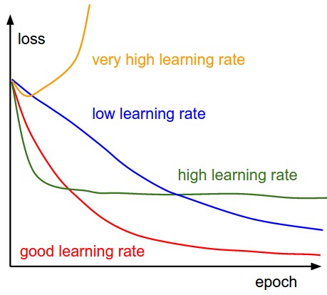
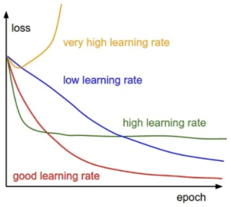
The loss curve over epochs reveals learning rate quality:
- Low learning rates → slow, nearly linear decay.
- High learning rates → rapid initial improvement, but poor convergence.
- Very high rates → chaotic oscillation.
-
The following figure shows the effects of different learning rates. With low learning rates the improvements will be linear. With high learning rates they will start to look more exponential. Higher learning rates will decay the loss faster, but they get stuck at worse values of loss (green line). This is because there is too much “energy” in the optimization and the parameters are bouncing around chaotically, unable to settle in a nice spot in the optimization landscape.
- The following figure shows: a typical CIFAR-10 loss curve (right). Left: A cartoon depicting the effects of different learning rates. An example of a typical loss function over time, while training a small network on CIFAR-10 dataset. This loss function looks reasonable (it might indicate a slightly too small learning rate based on its speed of decay, but it’s hard to say), and also indicates that the batch size might be a little too low (since the cost is a little too noisy).
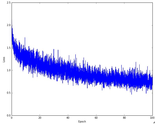
- The amount of stochastic “wiggle” depends on batch size: smaller batches → noisier curves.
Training vs. Validation Accuracy
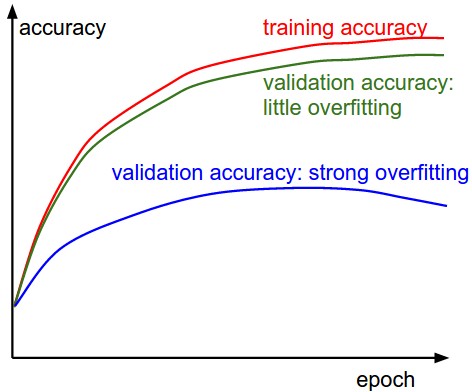
- Validation accuracy compared to training accuracy reveals overfitting: if training accuracy continues to rise while validation accuracy stagnates or declines, the model is memorizing noise rather than learning generalizable patterns.
-
This gap quantifies the generalization error, which reflects how well the learned function approximates the true underlying distribution. A large discrepancy usually indicates excessive model capacity or insufficient regularization, whereas closely tracking curves suggest either a well-regularized model or one that is underfitting due to limited expressiveness.
- The following figure shows two cases: (1) strong overfitting where validation accuracy lags far behind, and (2) under-capacity models where validation accuracy tracks training accuracy but remains low. Specifically, the gap between the training and validation accuracy indicates the amount of overfitting. Two possible cases are shown in the diagram on the left. The blue validation error curve shows very small validation accuracy compared to the training accuracy, indicating strong overfitting (note, it’s possible for the validation accuracy to even start to go down after some point). When you see this in practice you probably want to increase regularization (stronger L2 weight penalty, more dropout, etc.) or collect more data. The other possible case is when the validation accuracy tracks the training accuracy fairly well. This case indicates that your model capacity is not high enough: make the model larger by increasing the number of parameters.
Ratio of Updates to Weights
- A good heuristic is:
- If this ratio is too small, the learning rate is likely too low; if too high, the learning rate is unstable.
Activation / Gradient Distributions
- Plotting histograms of activations and gradients can diagnose poor initialization. For example,
tanhactivations should spread across[-1, 1]; if they collapse near 0 or saturate at extremes, initialization is flawed.
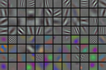
First-Layer Visualizations
- Visualizing learned filters is especially useful in image models: the first-layer filters often resemble Gabor-like edge detectors or color blobs, indicating that the network is extracting low-level visual primitives similar to those in biological vision. If instead the filters appear noisy or lack structure, it usually signals issues such as an excessively high learning rate, poor initialization, or overly strong regularization.
- Over time, clean and interpretable filters provide reassurance that the optimization process is progressing in a healthy direction, while incoherent filters suggest the model is failing to capture meaningful patterns from the input.
- The following figure shows first-layer weights with noisy features due to poor learning rate or regularization indicating an unconverged network.

- The following figure shows first-layer weights but with nice, smooth, clean and diverse features indicating healthy training, which are a good indication that the training is proceeding well.
Optimization
- Optimization lies at the heart of neural network training. While Stochastic Gradient Descent (SGD) is the foundation, its limitations in high-dimensional loss landscapes motivate more sophisticated approaches. In this section, we integrate theoretical perspectives with practical considerations, showing how modern optimizers overcome the shortcomings of vanilla SGD.
Problems with Stochastic Gradient Descent (SGD)
- Vanilla SGD updates parameters via:
- This is efficient, but several fundamental issues arise:
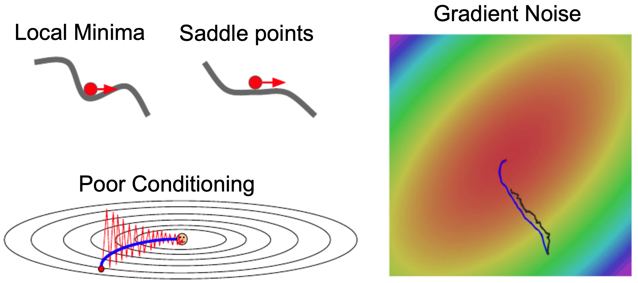
- Poor conditioning
-
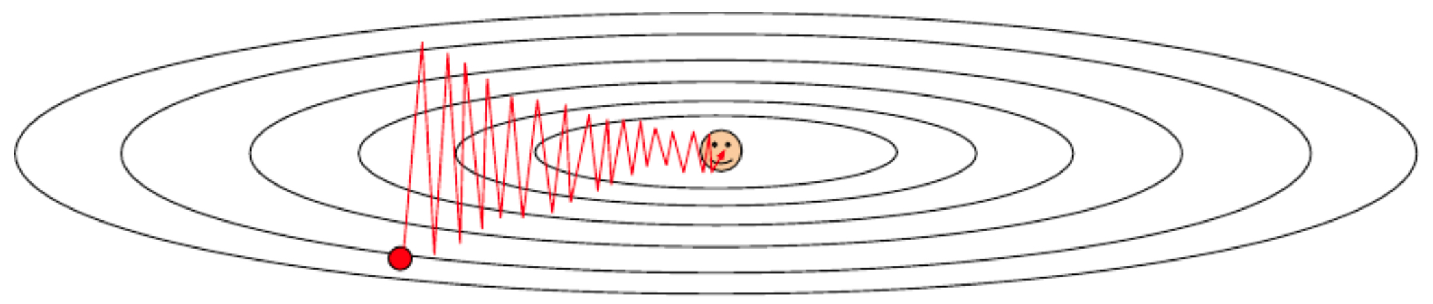
If the loss function changes steeply along one direction and slowly along another, optimization can zig-zag rather than progress directly toward the minimum. This effect is tied to the condition number of the Hessian (the ratio of its largest to smallest eigenvalue).
-
The following figure shows a contour plot of a poorly conditioned loss function, where the vertical direction is much more sensitive than the horizontal. An SGD update (red arrow) illustrates the inefficiency.
-
- Saddle points and local minima
-
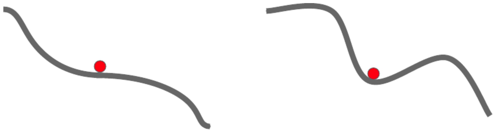
In high-dimensional spaces, saddle points (where gradients vanish but curvature has both positive and negative directions) are more problematic than local minima. SGD can stall near such points due to very small gradients (Dauphin et al., 2014).
-
The following figure shows how the gradient vanishes at a saddle point (left) and a local minimum (right), stalling progress.
-
- Mini-batch gradient noise
-
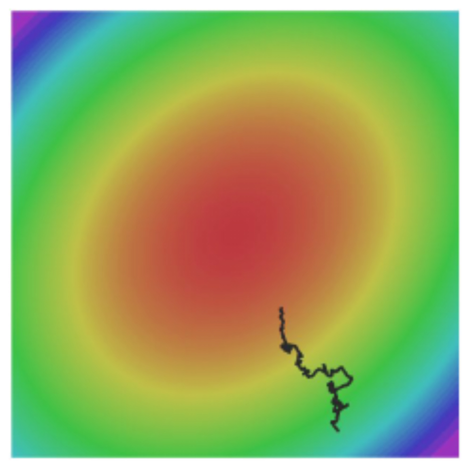
Since mini-batches only approximate the full gradient, SGD may take noisy, skewed steps that delay convergence.
-
The following figure shows potential update directions when the batch gradient is only a rough estimate of the full-data gradient.
-
- Together, these challenges explain why plain SGD is often too unstable for modern deep networks.
SGD with Momentum
-
Momentum introduces a velocity term that accumulates past gradients:
\[v_t = \rho v_{t-1} + \nabla L(w_t), \quad w_{t+1} = w_t - \alpha v_t\]- where, \(\rho\) (typically 0.9 or 0.99) acts as a friction coefficient, smoothing noisy updates. Intuitively, this is like rolling a ball down a hill: once moving, the ball keeps going in the same direction, making it less sensitive to local irregularities.
-
The following figure illustrates how momentum helps overcome saddle points, poor conditioning, and noisy gradients by averaging past updates. Starting in the upper left, we can think of a local minima and a saddle point as a ball rolling down a hill, where the height of the hill is the loss and the ball is the weights. As the ball rolls, it picks up velocity, and once it reaches its local minimum value, it will still continue to move due to the velocity it picked up. For the other examples of poor conditioning and gradient noise, the velocity term will take the weighted average, in each direction, for which the weights have previously moved; thus, in each direction the weights will move in a more direct path towards the minimum.
Nesterov Momentum
- Nesterov Accelerated Gradient (NAG) improves momentum by computing the gradient at a look-ahead position:
-
This anticipatory correction leads to more stable updates and less overshooting (Sutskever et al., 2013).
-
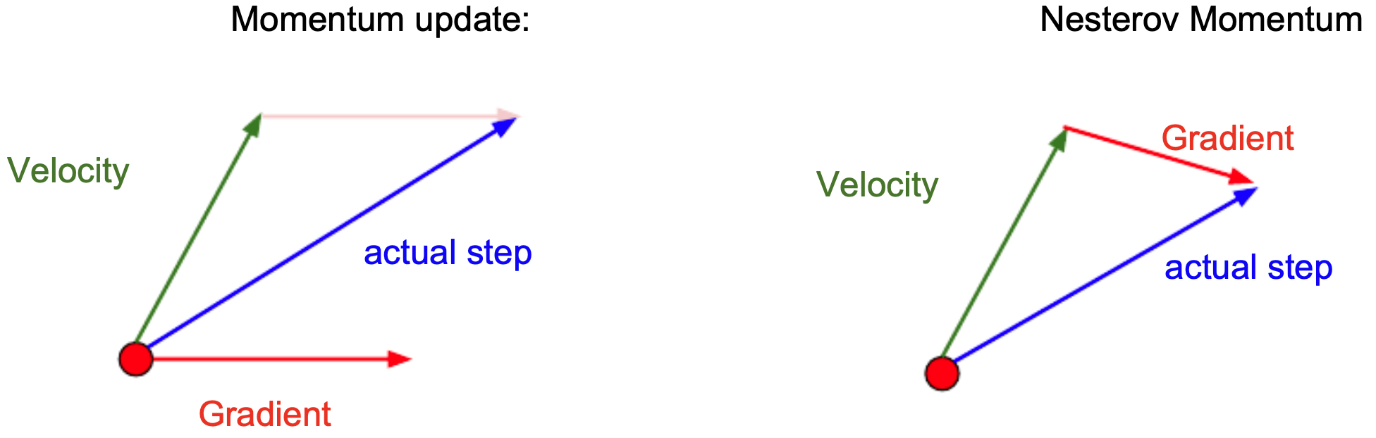
The following figure compares classical momentum (left) and Nesterov momentum (right). Momentum (left) calculates the gradient of the current weights and takes a step in the direciton combined from the directions of both the running velocity and the gradient. Nesterov momentum (right), by contrast, calculates the gradient from the veloctiy and then add that gradient to the velocity vector to form each step.
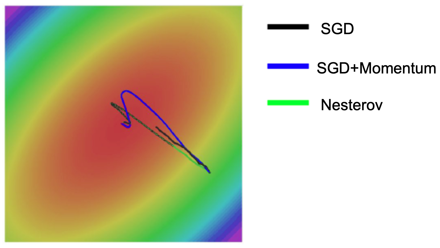
- The following figure compares the optimization paths of vanilla SGD, SGD with momentum, and Nesterov momentum. Notice that momentum often overshoots minima, while Nesterov provides finer control.
Adaptive Methods
AdaGrad
-
AdaGrad (Duchi et al., 2011) adapts the learning rate per parameter by dividing each update by the square root of the cumulative sum of squared gradients:
\[w_{t+1} = w_t - \frac{\alpha}{\sqrt{G_t + \epsilon}} \nabla L(w_t)\]- where \(G_t = \sum_{\tau=1}^t (\nabla L(w_\tau))^2\).
-
This allows larger steps in infrequently updated directions and smaller steps in frequently updated ones. However, the running sum grows without bound, eventually halting learning.
RMSProp
- RMSProp (Hinton, 2012) solves AdaGrad’s problem by using an exponential moving average of squared gradients:
-
This prevents the denominator from growing indefinitely and keeps updates adaptive throughout training.
-
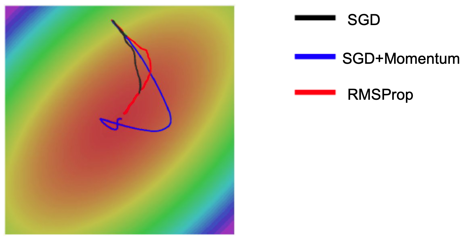
The following figure compares optimization trajectories of SGD, SGD with momentum, and RMSProp. Notice how RMSProp adapts better to saddle regions and poor conditioning.
Adam
- Adam (Kingma & Ba, 2014) combines momentum (first moment) with RMSProp (second moment):
- Bias-corrected estimates are then used for the update:
- The following figure shows convergence paths for SGD, SGD with momentum, RMSProp, and Adam. Adam combines the stability of RMSProp with the acceleration of momentum.
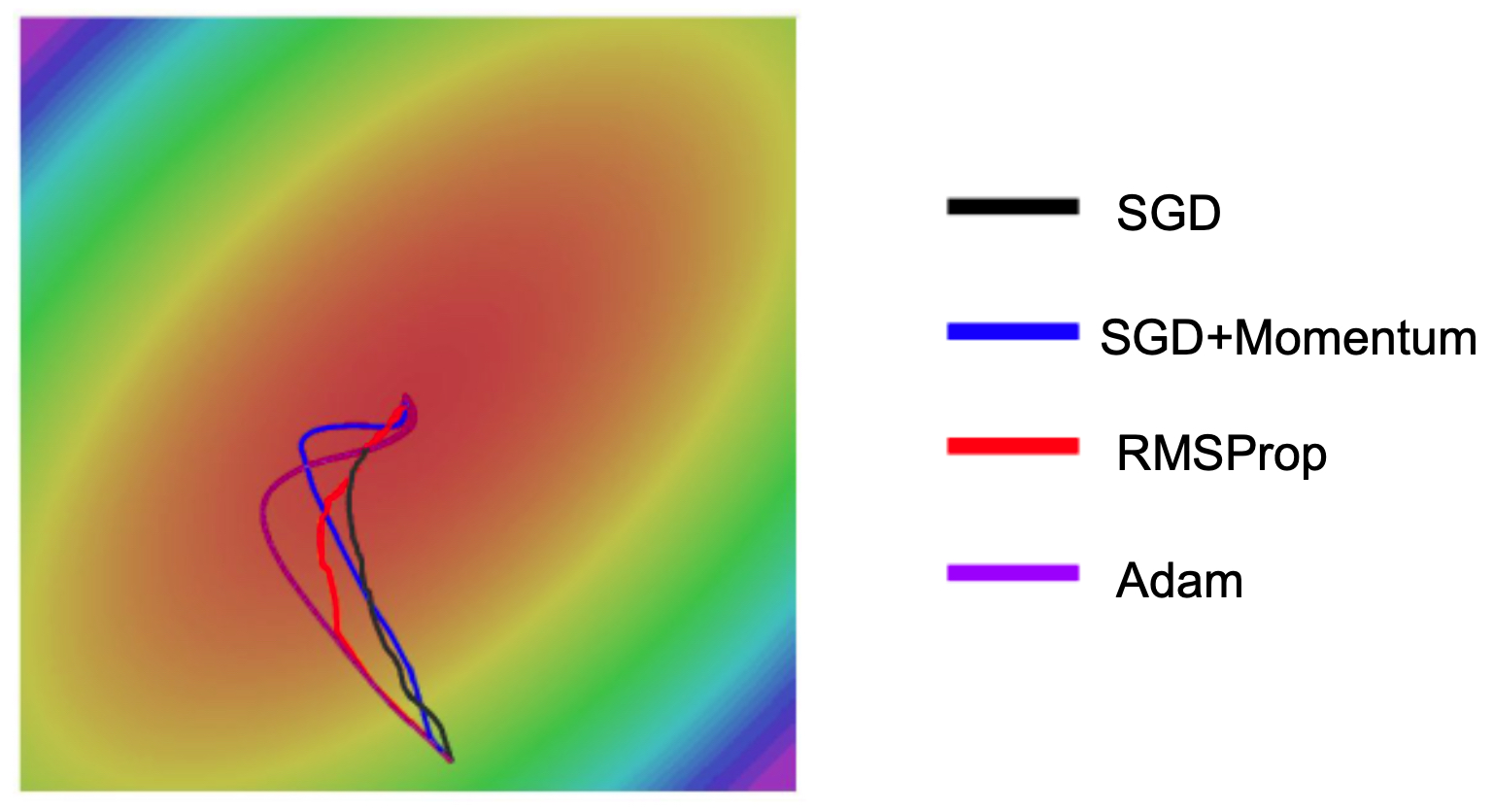
- Adam is often a strong default optimizer, though in practice, SGD with Nesterov momentum remains competitive when tuned carefully (Wilson et al., 2017).
Learning Rate Annealing
-
The learning rate greatly affects convergence:
- Step decay: halve every \(k\) epochs
- Exponential decay: \(\alpha_t = \alpha_0 e^{-kt}\)
- 1/t decay: \(\alpha_t = \frac{\alpha_0}{1+kt}\)
-
If decay is too slow, computation is wasted; if too aggressive, the model may converge to suboptimal minima.
-
The following figure shows how learning rates can be diagnosed by plotting loss curves. Flat decay suggests too small a rate, oscillation too large a rate, and smooth exponential-like decay a good rate.
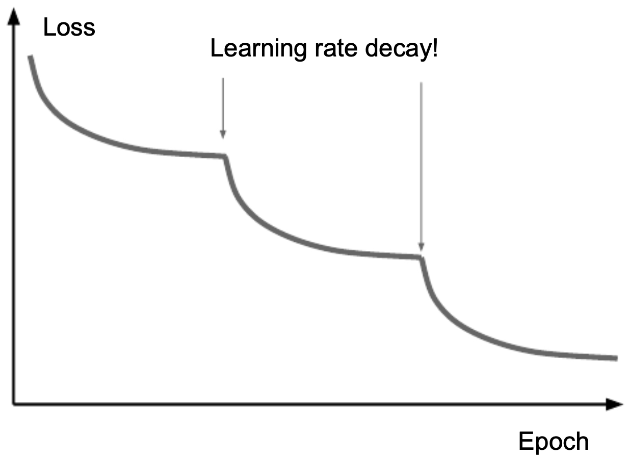
- The following figure illustrates the effect of learning rate decay: each time the rate is reduced, the loss drops in noticeable steps.
Second-Order Methods
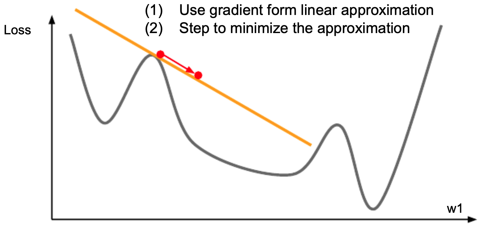
- The following figure illustrates the fact that with all the optimization techniques we have introduced thusfar, we have only looked at how the first order gradient can minimize the loss function.
-
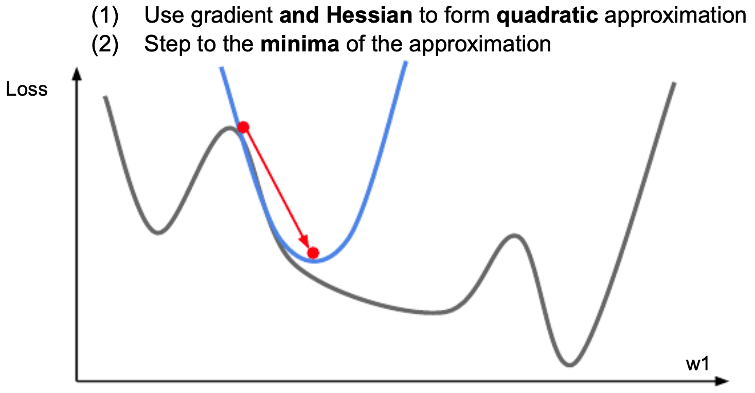
Newton’s method leverages curvature:
\[w_{t+1} = w_t - H^{-1} \nabla L(w_t)\]- where \(H\) is the Hessian. This update minimizes a quadratic approximation to the loss:
-
The following figure illustrates that using second-order optimization to step in the direction that minimizes the second order Taylor series of the loss function.
- While elegant, storing and inverting \(H\) is impractical for large models. Instead, quasi-Newton methods like BFGS and L-BFGS approximate curvature efficiently (Nocedal & Wright, 2006).
Adaptive Methods
-
Per-parameter adaptive methods adjust learning rates individually:
- AdaGrad (Duchi et al., 2011)
- RMSProp (Hinton, Coursera Lecture 6)
- Adam (Kingma & Ba, 2014)
-
The following figure presents an animation to build intuition about the learning process dynamics. It shows contours of a loss surface and time evolution of different optimization algorithms. Notice the “overshooting” behavior of momentum-based methods, which make the optimization look like a ball rolling down the hill.
- The following figure (source) shows a visualization of a saddle point in the optimization landscape, where the curvature along different dimension has different signs (one dimension curves up and another down). Notice that SGD has a very hard time breaking symmetry and gets stuck on the top. Conversely, algorithms such as RMSprop will see very low gradients in the saddle direction. Due to the denominator term in the RMSprop update, this will increase the effective learning rate along this direction, helping RMSProp proceed.: Left: optimization trajectories for different algorithms; Right: saddle point dynamics highlighting how RMSProp adapts learning rates.
- These methods form the backbone of modern deep learning optimization. Adam, in particular, has become the default optimizer, though SGD with Nesterov momentum remains a competitive alternative in practice.
Regularization
- As neural networks increase in size and capacity, they become prone to overfitting, where they memorize training data rather than learning generalizable patterns. Regularization combats this by constraining the model or augmenting data in ways that promote robustness. The general principle is that while regularization may slightly increase training error, it reduces validation error and improves real-world performance.
L2 Regularization (Weight Decay)
- L2 regularization adds a penalty proportional to the squared magnitude of weights:
- This discourages large weights, effectively reducing model complexity.
-
The gradient update for SGD with weight decay is:
\[w_{t+1} = (1 - \alpha \lambda)w_t - \alpha \nabla L_{\text{data}}\]- where weights shrink multiplicatively toward zero at every step, preventing runaway growth.
Dropout Regularization
-
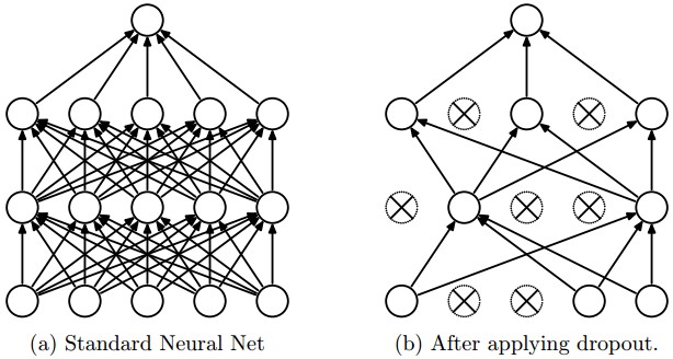
Dropout (Srivastava et al., 2014) is a stochastic regularization technique where neurons are randomly “dropped” (set to zero) during training with probability \(p\) (often 0.5). This prevents co-adaptation of features and forces the network to learn distributed representations. At test time, all neurons are active, but outputs are scaled to maintain consistency with training.
-
The following figure shows how dropout randomly removes neurons during training, effectively creating a different sub-network each iteration.
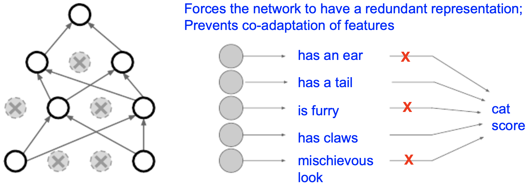
- The following figure illustrates how dropout prevents reliance on a single neuron. For example, a cat classifier might detect ears, fur, claws, and tail — dropout ensures redundancy by preventing overreliance on one feature.
-
Another interpretation of dropout is as an implicit ensemble method: each training pass samples a different sub-network, and their shared parameters average at test time. With 4096 units in a fully connected layer, dropout corresponds to training on an astronomical number of subnetworks (on the order of \(2^{4096} \approx 10^{1233}\)).
-
Inverted Dropout is the practical variant: during training, activations are scaled by \(1/p\) so that no rescaling is required at test time. This ensures that expectations remain consistent between phases.
Data Augmentation
-
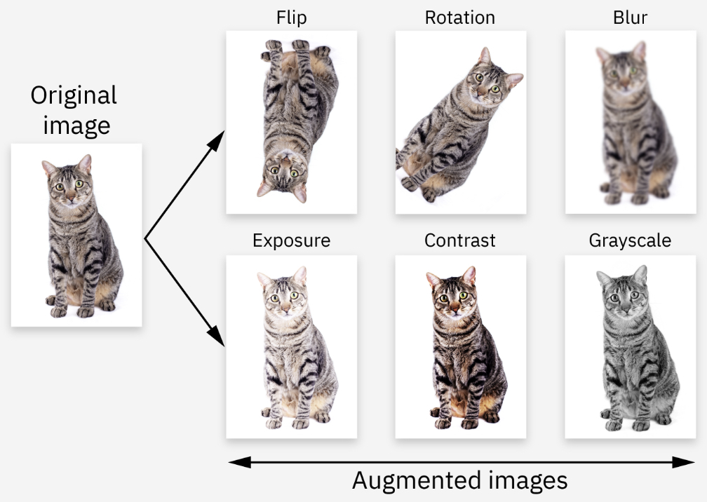
Data augmentation synthetically expands training data by applying transformations such as flips, random crops, rotations, scaling, and color jittering. This technique encourages networks to learn invariances (e.g., object identity is unchanged under horizontal flips).
-
The following figure (source) illustrates data augmentation: instead of training on the original image, the model sees transformed variants, improving generalization.
- In large-scale vision models (e.g., ResNet), augmentation pipelines include multi-scale resizing (224–640 pixels), multiple random crops per image, and horizontal flips. At test time, averages over a fixed number of crops ensure robustness.
Early Stopping
-
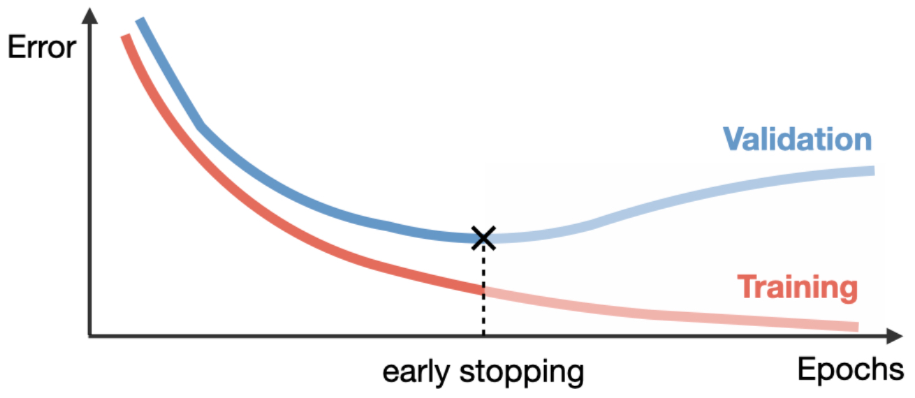
Training too long often causes validation error to rise while training error continues to fall. Early stopping halts training when validation loss stops improving, preventing overfitting.
-
The following figure shows validation loss diverging from training loss, with early stopping marking the point where generalization is maximized.
Other Regularization Methods
- Batch Normalization (BN) (Ioffe & Szegedy, 2015) normalizes intermediate activations, stabilizing training and allowing larger learning rates. It also acts as a mild regularizer.
- Data augmentation + BN often outperform explicit weight penalties in modern CNNs.
-
Sanity check for overfitting: Track training vs. validation curves — a widening gap signals overfitting, while both low indicates undercapacity.
- The following figure shows overfitting (large gap between training and validation accuracy) versus under-capacity (both accuracies low and closely tracking).
Ensemble-Averaged Regularization Perspective
-
Dropout and augmentation can both be reframed as ensemble methods:
- Dropout → implicit averaging of many subnetworks.
- Augmentation → averaging predictions across transformed inputs.
- Batch norm → reducing internal covariate shift, indirectly improving generalization.
-
Together, these regularization strategies enable deep networks to learn generalizable patterns even in limited or noisy data regimes.
Model Ensembles
- Another highly effective way to reduce generalization error is to average predictions from multiple models. Ensembles improve robustness by reducing variance, since individual model errors often cancel out. This approach is widely used in practice and is especially common in machine learning competitions, where ensemble methods often secure state-of-the-art performance.
Why Ensembles Work
- Each individual model trained on the same dataset makes slightly different errors due to random initialization, stochastic training, or architectural differences.
- Averaging their predictions smooths out idiosyncratic mistakes, yielding better generalization on unseen data.
- Ensembles also tend to improve stability, reducing sensitivity to hyperparameter choices.
Approaches to Ensembling
-
Several strategies exist for creating effective ensembles:
-
Independent Training
- Train the same architecture with different random initializations and average predictions.
- Computationally expensive, but often the most effective.
-
Hyperparameter Variants
- Keep architecture fixed but ensemble models trained with different hyperparameters (e.g., dropout rates, learning rates).
-
Checkpoints During Training (Snapshot Ensembles)
- Instead of training multiple models from scratch, save several checkpoints during a single training run (e.g., after different epochs).
- At test time, average predictions from these snapshots. This method reduces compute cost but still captures diversity.
-
Polyak Averaging (a.k.a. Weight Averaging)
- Instead of ensembling outputs, average model weights over time (Polyak & Juditsky, 1992).
- This yields smoother and often better-performing models than the final checkpoint alone.
- Stochastic Weight Averaging (SWA) (Izmailov et al., 2018) is a modern variant.
-
Computational Cost vs. Accuracy
-
While ensembles generally improve performance, they require extra compute at inference time, which can be prohibitive in real-world systems. To mitigate this:
- Knowledge Distillation (Hinton et al., 2015) can compress an ensemble into a single model by training a smaller “student” model on the predictions of the larger “teacher” ensemble.
- Averaging weights (e.g., Polyak or SWA) reduces inference cost while maintaining many of the benefits.
Takeaways
- Ensembles improve validation error more effectively than training error — they specifically target generalization.
- They can be built from multiple independent models, hyperparameter variants, snapshots, or weight averaging.
- While compute-intensive, ensembles remain one of the most reliable tools for boosting model performance.
- For deployment, distillation or averaging methods are often used to achieve ensemble-like performance without ensemble-level cost.
Hyperparameter Tuning
- Hyperparameters are the external settings of a neural network that cannot be directly learned from data — such as the learning rate, regularization strength, dropout probability, and network architecture. Choosing them well is crucial, as they strongly influence both convergence speed and final performance.
Manual Search
- The simplest strategy is manual tuning, guided by practitioner intuition. While sometimes effective for experienced researchers, it is inefficient and error-prone, especially for large-scale models with many interacting hyperparameters. Manual search is best reserved for quick debugging or when computational resources are limited.
Grid Search
- Grid search systematically evaluates all possible combinations of hyperparameters within a fixed range. While exhaustive, it suffers from the curse of dimensionality: the number of evaluations grows exponentially with the number of parameters. Additionally, grid search wastes effort testing unimportant hyperparameters.
Random Search
-
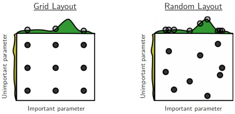
Random search (Bergstra & Bengio, 2012) samples hyperparameters from probability distributions rather than evaluating all combinations. This often works better in practice because:
- Only a few hyperparameters (e.g., learning rate, weight decay) usually dominate performance.
- Random sampling explores these influential hyperparameters more effectively.
- It avoids wasting compute on combinations of irrelevant hyperparameters.
-
The following figure illustrates why random search is typically superior to grid search. Grid search may miss the critical region entirely, while random search is more likely to discover high-performing configurations.
Practical Tips for Hyperparameter Search
-
Log-scale sampling Sample hyperparameters like learning rate or weight decay on a log scale (e.g., \(10^{U[-6,1]}\)) since their effects are multiplicative.
-
Stage search from coarse to fine Start with broad ranges and short training runs (1–2 epochs) to identify promising regions. Then refine with narrower ranges and longer runs.
-
Check boundaries If the best value lies on the edge of the search space, expand the range.
-
Validation splits For large datasets, a single validation set suffices (cross-validation is rarely necessary).
-
Parallelization Distribute hyperparameter trials across multiple workers. A worker–master setup is common: workers train independently, while the master monitors results and updates the search.
Bayesian Optimization
-
Beyond random search, Bayesian optimization (Snoek et al., 2012) models the performance landscape of hyperparameters probabilistically, using acquisition functions (e.g., expected improvement) to balance exploration and exploitation.
-
Several libraries implement Bayesian optimization, including:
-
Despite its sophistication, in practice, carefully staged random search often rivals or outperforms Bayesian methods in convolutional networks. This is due to the simplicity of the underlying performance landscape and the fact that only a handful of hyperparameters usually matter.
Takeaways
- Manual search is quick but unreliable.
- Grid search is exhaustive but computationally prohibitive.
- Random search strikes a strong balance between simplicity and effectiveness.
- Bayesian methods can be more efficient in certain cases, but staged random search often suffices in practice.
Softmax and Cross-Entropy
- For multi-class classification tasks, neural networks typically output raw scores (logits) for each class. To convert these into probabilities, we use the Softmax function.
Softmax Function
- Given logits \(f_i\) for each class \(i\), the Softmax function is defined as:
-
Properties of Softmax:
- Each \(S_i \in [0,1]\), so outputs can be interpreted as probabilities.
- The probabilities sum to 1, making it a valid distribution:
- Adding a constant \(c\) to all logits does not change the result (important for numerical stability). This allows us to subtract the maximum logit before exponentiation to prevent overflow.
Cross-Entropy Loss
-
Once logits are mapped to probabilities via Softmax, we use Cross-Entropy (CE) loss to measure discrepancy between the predicted distribution \(q(y)\) and the true distribution \(p(y)\) (one-hot encoded label):
\[L = - \sum_i y_i \log S_i\]- where \(y_i = 1\) if \(i\) is the correct class, and \(0\) otherwise. Minimizing CE encourages the model to assign higher probability to the correct class.
-
Cross-Entropy is preferred over alternatives like Mean Squared Error (MSE) for classification because it provides stronger gradients, especially when predictions are very wrong.
Information-Theoretic Perspective
- The pairing of Softmax and Cross-Entropy is not arbitrary — it is grounded in information theory.
- Entropy
- The entropy of a true distribution \(p(y)\) is:
- It quantifies the inherent uncertainty of predicting \(y\).
- Cross-Entropy
- Cross-Entropy between distributions \(p\) and \(q\) is:
- It represents the expected number of bits required to encode samples from \(p\) using a code optimized for \(q\).
- KL Divergence
- Cross-Entropy decomposes as:
-
where:
\[D_{KL}(p \parallel q) = \sum_i p(y_i) \log \frac{p(y_i)}{q(y_i)}\] -
Minimizing Cross-Entropy is equivalent to minimizing KL divergence, pushing predictions \(q\) closer to the true labels \(p\).
- Softmax as Maximum Entropy Distribution
- Softmax arises naturally when seeking the maximum entropy distribution under linear constraints on expected scores. It is the least biased distribution consistent with the given logits, consistent with Jaynes’ maximum entropy principle.
Practical Considerations
- Numerical stability: In practice, logits are shifted by subtracting their maximum value before exponentiation.
- Label smoothing: Instead of using one-hot labels, target distributions can be smoothed (e.g., assigning \(0.9\) to the correct class and distributing \(0.1\) across others). This regularizes the model, preventing it from becoming overconfident (Szegedy et al., 2016).
- Large vocabularies: In language models with very large output spaces (tens of thousands of tokens), computing the full Softmax is expensive. Techniques such as hierarchical Softmax, sampled Softmax, or Noise-Contrastive Estimation (NCE) are used to approximate it.
Intuitive Link
- Softmax ensures outputs are interpretable as probabilities.
- Cross-Entropy measures the coding inefficiency of predictions compared to the true distribution.
-
Together, they frame classification learning as minimizing the expected extra coding cost of using predicted probabilities instead of the true distribution.
- This elegant link between statistical learning and information theory explains why Softmax + Cross-Entropy has become the canonical choice for classification in deep learning.
Transfer Learning
- Modern deep learning models are typically pretrained on massive datasets such as ImageNet (vision), COCO (detection), or large text corpora (e.g., BERT, GPT). These pretrained models learn general-purpose representations that can be adapted to new tasks with relatively little data. This process, known as transfer learning, has become the standard practice across domains.
- Transfer learning has shifted from being a specialized technique to the default paradigm in deep learning. For most practical tasks, training from scratch is unnecessary. Instead, pretrained models are adapted to new domains, saving computation and data while achieving higher accuracy and stability.
Why Transfer Learning Works
- Hierarchical feature learning: Early layers capture universal patterns such as edges, textures, and shapes, while later layers capture higher-level task-specific semantics (e.g., objects, categories).
- Representation reuse: When adapting to a new dataset, much of the low- and mid-level representation remains useful; only higher layers need major adaptation.
- Data efficiency: Training from scratch often requires millions of labeled examples. Transfer learning allows strong results with far fewer.
- Regularization via pretraining: Pretrained weights encode useful priors, preventing overfitting in small-data regimes.
Typical Workflow
-
Pretraining Train a model on a large-scale dataset (e.g., ImageNet, Wikipedia, LAION).
-
Freezing Freeze earlier layers, which act as fixed feature extractors, and replace the classifier head with a new randomly initialized layer.
-
Fine-tuning
- With very little data: Train only the new head.
- With more data: Progressively unfreeze and fine-tune earlier layers.
- With large or distant-domain datasets: Retrain most or all layers, often with differential learning rates.
- The following figure illustrates this workflow: pretrained layers are frozen while later layers are reinitialized and retrained. With larger target datasets, progressively more layers can be fine-tuned.

Strategies for Fine-Tuning
-
Feature Extraction Mode Keep the backbone frozen and train only a shallow classifier head. Works best for very small, similar datasets.
-
Partial Fine-Tuning Unfreeze the top few layers of the network. Balances stability with flexibility, suitable for moderately sized datasets.
-
Full Fine-Tuning Unfreeze all layers and retrain end-to-end. Necessary for large datasets or when the new domain is very different from the pretraining dataset.
Guide to Choosing a Transfer Learning Strategy
- The following figure illustrates how to choose a transfer learning strategy depending on dataset size and similarity.
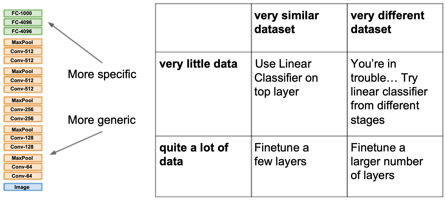
- The table below provides a more detailed summary of trade-offs between dataset size and similarity to pretraining. When the dataset is small and dissimilar, transfer learning becomes more challenging, and alternative approaches (semi-supervised learning, synthetic data, or stronger augmentation) may be required.
| Data Regime / Dataset Similarity | Very Similar Dataset (close domain) | Very Different Dataset (distant domain) |
|---|---|---|
| Very Little Data | Use a linear classifier on top of pretrained features. Freeze the entire backbone (convolutional or transformer layers) and only train a small classifier head. Since the features are already well aligned with your task, this avoids overfitting and provides strong performance with minimal data. | Try linear classifiers from different stages of the network. Earlier layers capture more generic patterns (edges, textures), while later layers encode task-specific semantics. In low-data, cross-domain settings, probing different layers can help identify which features transfer best. |
| Moderate Amount of Data | Fine-tune the top few layers. Keep most of the backbone frozen, but allow the last block(s) to adapt to task-specific patterns. This balances stability with flexibility, requiring fewer parameters to update while still adapting to the new dataset. | Progressively unfreeze deeper layers. Start with the classifier and top layers, then gradually unfreeze more layers while monitoring validation loss. This mitigates catastrophic forgetting and allows adaptation to the new domain when moderate data is available. |
| Quite a Lot of Data | Fine-tune many or all layers. With sufficient data in a similar domain, updating most of the pretrained network yields the best results. Pretraining still provides a head start, but the model can now fully adapt. | Full fine-tuning is often required. When the dataset is both large and very different, the pretrained features may not align well. Fine-tune all layers, sometimes with a lower learning rate for earlier layers (to preserve general features) and a higher rate for later ones. |
| Extremely Large Data | From-scratch training becomes viable. Pretraining is still helpful for initialization, but with huge in-domain data, training from scratch may match or surpass transfer learning. | Pretraining may be less relevant. For entirely new domains and massive datasets, initializing randomly and training fully can be competitive, though pretraining often accelerates convergence and improves early stability. |
Transfer Learning in Practice
- Learning Rate Scheduling: Fine-tuned layers often require a smaller learning rate than newly initialized layers to avoid catastrophic forgetting. Differential learning rates (e.g., base LR for new layers, 1/10 LR for pretrained layers) are common.
- Regularization: Dropout, weight decay, and augmentation remain critical when fine-tuning on small datasets.
- Layer Freezing Strategies: Progressive unfreezing (gradually unfreezing earlier layers over training epochs) improves stability.
- Cross-Domain Applications: Especially impactful where labeled data is scarce — e.g., medical imaging, genomics, and speech recognition.
Broader Perspective: Transfer Learning vs. Pretraining Paradigms
- Feature-based Transfer: Use pretrained embeddings (e.g., word2vec, CLIP) as input features for simpler downstream models.
- Fine-tuning Transfer: Jointly adapt pretrained weights during training.
- Zero-shot and Few-shot Transfer: Enabled by large foundation models (e.g., GPT, CLIP, Flamingo), which can directly generalize to new tasks with minimal or no fine-tuning.
Putting It All Together: A Recipe for Training Neural Networks
-
Training a modern neural network is as much an art as it is a science. The preceding sections covered the building blocks — optimization methods, regularization strategies, hyperparameter tuning, and transfer learning. Success in practice requires orchestrating these pieces into a systematic workflow that guides you from data preprocessing to final evaluation and deployment.
-
This recipe is not a rigid protocol, but a scaffold for experimentation. Each dataset, model architecture, and application domain presents unique challenges. By combining the principles of optimization, regularization, and transfer learning with careful monitoring and iteration, one can navigate the messy realities of training neural networks and consistently arrive at effective, generalizable solutions.
Preprocessing
- Zero-centering: Subtract the dataset-wide mean (image or feature mean) from each input, ensuring data is centered at zero.
- Normalization: Scale features to have unit variance. For images, normalize each RGB channel using dataset-wide statistics.
-
Data augmentation: Apply label-preserving transformations to increase robustness and effective dataset size. For images: flips, random crops, rotations, and color jitter; for text: back-translation, masking, or synonym replacement.
- These steps align the input data with the assumptions of optimization algorithms and reduce overfitting by expanding data diversity.
Training
- Mini-batching: Use mini-batches (32, 64, 128, etc.) for stochastic gradient updates. This balances computational efficiency with gradient stability.
- Optimizer: Begin with Adam (robust and adaptive) or SGD + Nesterov momentum (often yields better generalization if tuned well).
- Learning rate schedules: Use decay strategies such as step decay, exponential decay, or cosine annealing. Avoid premature use of decay; first identify a good base learning rate, then apply decay once validation performance plateaus.
Regularization
- L2 weight decay: Penalizes large weights, encouraging simpler models.
- Dropout: Randomly deactivate neurons during training to reduce co-adaptation.
- Batch normalization: Normalizes intermediate activations, acting as both stabilizer and mild regularizer.
-
Early stopping: Halt training when validation loss ceases to improve, preventing overfitting.
- These methods, when combined, ensure robustness and stability across both small and large datasets.
Evaluation
- Train/validation split: Always monitor both training and validation curves. Training accuracy reflects fit; validation accuracy reflects generalization.
- Overfitting check: A widening gap between training and validation accuracy indicates overfitting; apply stronger regularization or acquire more data.
- Small-data sanity check: Verify that the model can overfit a tiny dataset (e.g., 20 examples). Failure here suggests implementation errors.
Babysitting the Training Process
-
Training is rarely smooth. Diagnostics provide windows into optimization health:
- Loss curves: Smooth exponential-like decay is typical. Oscillation suggests a learning rate that is too high or a batch size that is too small.
- Validation accuracy: Track alongside training accuracy. A widening gap signals overfitting.
- Update-to-weight ratio: Monitor \(\frac{\|\Delta w\|}{\|w\|} \approx 10^{-3}\). Too low → learning rate is too small; too high → unstable optimization.
- Activation/gradient distributions: Watch for saturation or collapse. Healthy networks show diverse activations.
- First-layer filter visualization: For vision models, filters should evolve into smooth, interpretable edge and texture detectors. Persistent noise indicates optimization issues.
Ensemble for Robustness
-
Once a single model is trained, performance can often be boosted by ensembling:
- Combine multiple independently trained models.
- Average checkpoints from different training epochs (snapshot ensembling).
- Use parameter averaging strategies such as Polyak averaging (exponential moving averages).
-
Ensembling reduces variance and typically improves robustness, though at the cost of additional inference computation.
Summary Workflow
- Preprocess your data: normalize, augment, and zero-center.
- Initialize your model: perform gradient checks and sanity checks before training.
- Train with an adaptive optimizer and a sensible learning rate schedule.
- Regularize with weight decay, dropout, batch norm, and early stopping.
- Monitor training carefully: loss curves, accuracy gaps, update ratios, and filter visualizations.
- Ensemble or fine-tune for final robustness before deployment.
Further Reading
- Yosinski et al., 2014: “How transferable are features in deep neural networks?” — foundational empirical study showing early layers are more general, later layers more task-specific.
- Donahue et al., 2014: “DeCAF” — early work demonstrating CNN features pretrained on ImageNet transfer well to many tasks.
- Howard & Ruder, 2018: “ULMFiT” — breakthrough in NLP transfer learning with fine-tuned LSTM language models.
- Radford et al., 2021: “CLIP” — multimodal transfer learning model generalizing across vision and language.
Citation
If you found our work useful, please cite it as:
@article{Chadha2020TrainingNeuralNetworksII,
  title   = {Training Neural Networks II},
  author  = {Chadha, Aman},
  journal = {Distilled Notes for Stanford CS231n: Convolutional Neural Networks for Visual Recognition},
  year    = {2020},
  note    = {\url{https://aman.ai}}
}