CS231n • Training Neural Networks I
- Overview
- Activation Functions
- Data Preprocessing
- Weight Initialization
- Batch Normalization
- Training Neural Networks: A Case Study
- Citation
Overview
-
Training deep neural networks involves more than simply stacking layers of neurons together. For networks to learn effectively, several design principles must be carefully chosen and combined. This primer introduce these principles, covering activation functions, preprocessing, weight initialization, normalization, and their integration into a training pipeline.
-
Activation functions: Neural networks derive their expressive power from non-linearities interwoven between linear transformations. Without them, networks collapse into a single linear mapping, regardless of depth. Choosing the right activation function — from classic sigmoids and tanh to modern ReLU variants and Maxout — directly affects convergence, stability, and representational capacity.
-
Data preprocessing: Proper preprocessing ensures that inputs are well-conditioned for learning. Techniques such as mean subtraction, normalization, and (historically) PCA/whitening center and rescale data to prevent skewed gradients. In computer vision, preprocessing often reduces to subtracting dataset or per-channel means, while PCA is rarely applied in convolutional settings.
-
Weight initialization: Initialization strongly influences whether signals propagate effectively through a network. Poor initialization can cause gradients to vanish or explode, stalling learning. Strategies like Xavier initialization (for symmetric activations) and He initialization (for ReLUs) calibrate variance across layers, breaking symmetry while maintaining stable signal flow.
-
Batch normalization: Introduced to counter internal covariate shift, batch normalization stabilizes activations within each mini-batch. It allows for higher learning rates, reduces the need for meticulous initialization, and provides a regularization effect. Today, BN is a standard component of most deep architectures.
-
Case study: training loop: These components come together in a practical pipeline. Data is zero-centered, weights are carefully initialized, activations are chosen to balance expressivity and stability, and batch normalization stabilizes learning. With these foundations, networks can be trained reliably using iterative forward and backward passes guided by loss minimization.
-
-
Together, these elements form the foundation of deep learning practice. Without them, training modern architectures would be prohibitively unstable or slow. The following sections examine each component in detail, motivating their necessity and exploring their impact on effective learning.
Activation Functions
-
Training deep neural networks requires the use of non-linear activation functions. Without them, no matter how many layers are stacked, the network behaves as a single linear transformation, which severely restricts its representational power. Activation functions introduce the non-linearity that allows networks to approximate arbitrarily complex functions (see Cybenko, 1989, Hornik, 1991).
-
The following figure presents the most common activation functions used in practice, highlighting their functional forms and typical ranges of output values.
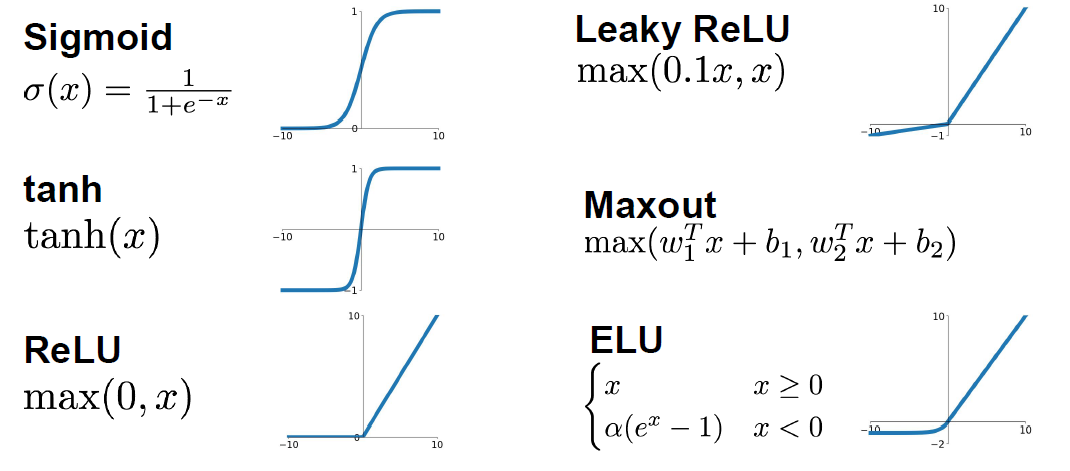
Sigmoid
- The sigmoid function is defined as:
-
This maps real numbers to the range (0,1). It has historically been widely used (Rumelhart et al., 1986) because its probabilistic interpretation made it intuitive for neuron firing rates and output probabilities. However, it suffers from several issues:
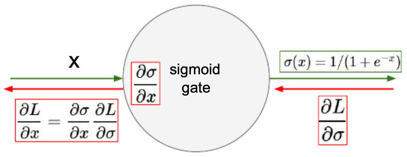
- Vanishing gradients: For very large positive or negative inputs, the derivative approaches zero, halting learning in deeper layers. The following figure illustrates this effect, showing how chaining layers together multiplies near-zero gradients until they vanish.
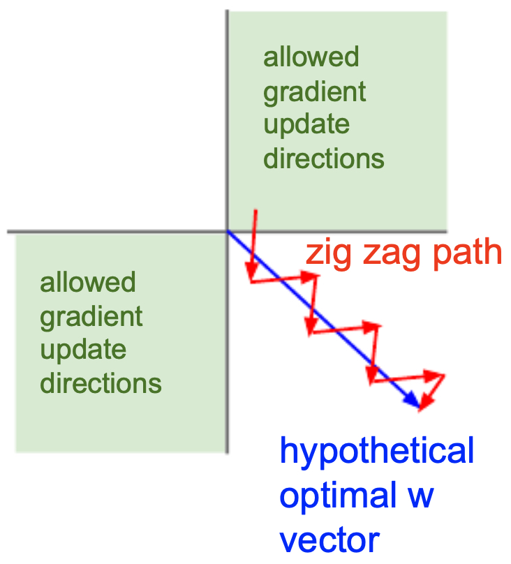
- Not zero-centered: Sigmoid outputs lie strictly in
(0,1). As a result, weight updates during backpropagation are always either all positive or all negative, leading to inefficient zig-zagging gradient descent paths instead of smooth convergence.
- The following figure shows how sigmoid non-zero-centered outputs constrain gradient directions, creating inefficient zig-zag descent paths. Put simply, the gradient of our weights will only ever be all positive or all negative when using a sigmoid activation function that has all positive inputs.
- Computational overhead: Exponentiation in the sigmoid is more expensive than simple piecewise linear functions like ReLU. Although this is small compared to matrix multiplications in neural nets, it adds up at scale.
Hyperbolic Tangent (Tanh)
- The tanh function is defined as:
- or equivalently:
- Tanh outputs lie in
(-1,1), making it zero-centered, which helps during backpropagation by allowing gradients to flow in both positive and negative directions. This avoids the all-positive/all-negative gradient issue seen in sigmoids. However, tanh still suffers from gradient saturation at the tails and requires exponentiation, which is computationally more expensive than ReLU.
Rectified Linear Unit (ReLU)
- The ReLU function is defined as:
-
First proposed in deep learning contexts by (Nair & Hinton, 2010), ReLU became the default nonlinearity because of several advantages:
- Computationally efficient (only a comparison and maximum).
- Does not saturate in the positive region, mitigating the vanishing gradient problem.
- Converges faster in practice than sigmoid or tanh.
- Biologically inspired: resembles neuronal firing thresholds.
-
However, ReLU is not zero-centered, and with negative inputs the gradient is zero. If poorly initialized, neurons can output only zeros, leading to the dying ReLU problem. A common workaround is initializing biases to small positive values (e.g., 0.01).
ReLU Variants
-
To address dying ReLUs, several variants were introduced:
-
Leaky ReLU: \(f(x) = \max(\alpha x, x), \quad \alpha \approx 0.01\) Allows a small gradient for negative inputs.
-
Parametric ReLU (PReLU): Same as Leaky ReLU, but \(\alpha\) is learned during training (He et al., 2015).
-
Exponential Linear Unit (ELU): \(f(x) = \begin{cases} x & \text{if } x \geq 0 \\ \alpha(e^x - 1) & \text{if } x < 0 \end{cases}\) ELUs push the mean activation closer to zero and are more robust to noise, but require exponentiation.
-
-
These variants improve representational capacity while reducing dead neurons.
Maxout
- The Maxout neuron (Goodfellow et al., 2013) generalizes ReLU by taking the maximum over multiple affine functions:
- Maxout learns its own activation function shape and avoids saturation or dying neurons. However, it doubles or multiplies parameter count (depending on k), making it computationally expensive. Despite these costs, it has strong theoretical justification as a universal approximator for activation functions.
Data Preprocessing
-
Before training, data must be normalized to ensure stability and efficiency. Without preprocessing, gradients can become unbalanced, leading to slow convergence or divergence during optimization. Proper preprocessing ensures that inputs are well-scaled and centered, allowing the network to learn more effectively (LeCun et al., 1998).
-
In practice, preprocessing is typically applied to a data matrix \(X \in \mathbb{R}^{N \times D}\), where \(N\) is the number of samples and \(D\) their dimensionality.
Mean Subtraction
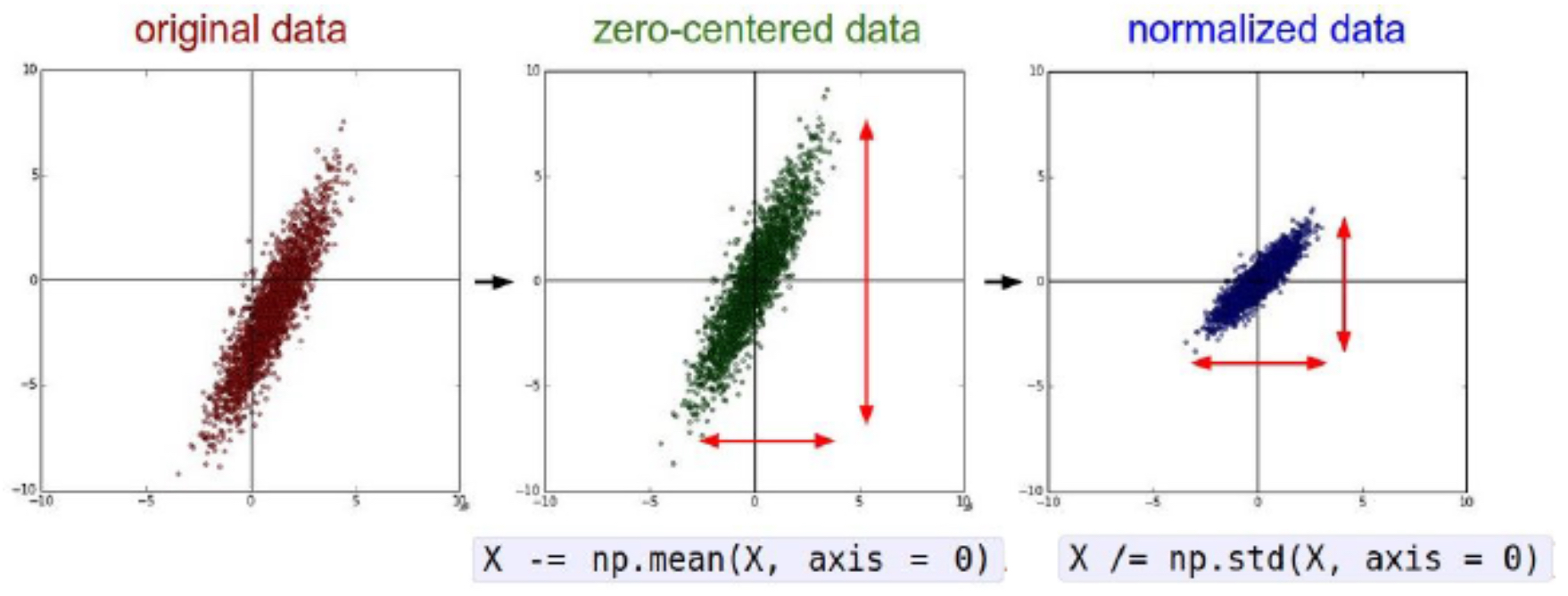
- The most common preprocessing step is mean subtraction. For each feature dimension, the mean is subtracted, centering the data around the origin:
X -= np.mean(X, axis = 0) # subtract feature-wise mean
-
For images, this often reduces to subtracting either:
- A single scalar mean across all pixels (as in AlexNet).
- Per-channel RGB means (as in VGGNet).
-
This ensures that input features are zero-centered. Importantly, the mean must be computed on the training set and consistently applied to validation and test sets to avoid data leakage.
Normalization
- Even after mean subtraction, different features may have very different variances. Normalization rescales each feature dimension to have comparable ranges:
X /= np.std(X, axis = 0) # standardize features
-
Alternatively, features can be scaled into bounded ranges such as
[-1,1]. For images, this step is often omitted since pixel values already occupy a fixed range (0–255). Still, centering pixel intensities around zero improves optimization. -
The following figure presents a common preprocessing step where data is normalized by subtracting the mean and dividing by the standard deviation. This ensures features are centered at zero and rescaled for stability.
PCA and Whitening
- Beyond standardization, Principal Component Analysis (PCA) and whitening can further normalize data. The covariance matrix of zero-centered data is
cov = np.dot(X.T, X) / X.shape[0]
- with eigenvectors computed via Singular Value Decomposition (SVD):
U, S, V = np.linalg.svd(cov)
- Projecting into the eigenbasis decorrelates features:
Xrot = np.dot(X, U) # rotate into eigenbasis
- Dimensionality reduction is achieved by keeping only the top eigenvectors:
Xrot_reduced = np.dot(X, U[:, :100]) # reduce to 100 dimensions
- Finally, whitening rescales each component by the inverse square root of its eigenvalue:
Xwhite = Xrot / np.sqrt(S + 1e-5)
- The following figure shows PCA and whitening on a toy dataset. Left: original correlated features. Middle: PCA rotation decorrelates them. Right: whitening rescales to unit variance in all directions.
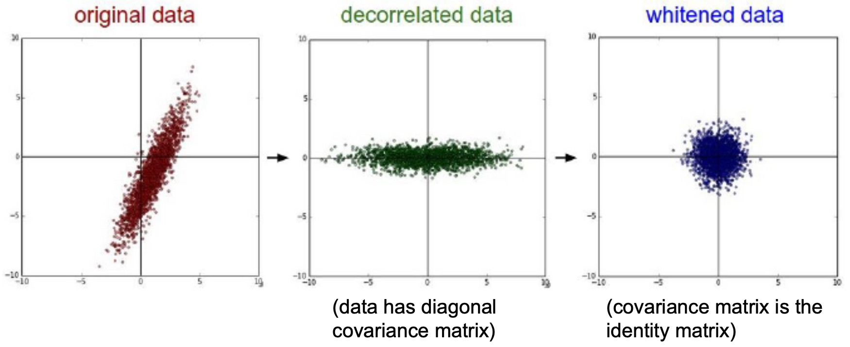
- Whitening produces zero-mean, identity-covariance data but may amplify noise in low-variance components.
PCA on Images
-
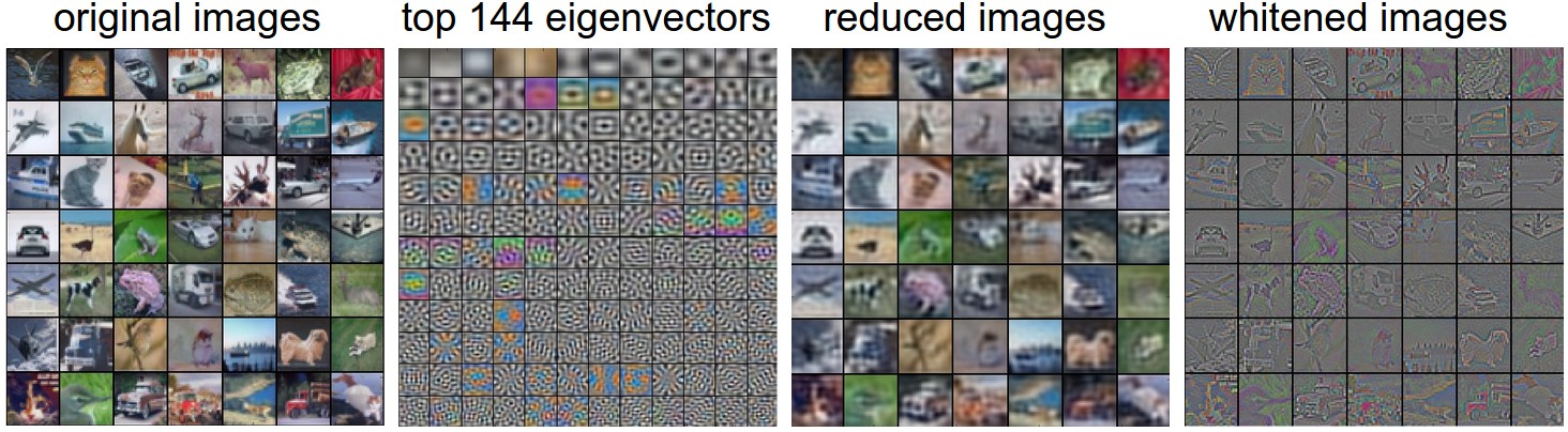
When PCA is applied to image datasets such as CIFAR-10, the top eigenvectors correspond to smooth, low-frequency structures (broad color blobs and edges), while high-frequency components contribute little variance. This explains why retaining a modest number of principal components preserves much of the structure.
-
The following figure illustrates PCA on CIFAR-10. Left: original images. Second from left: eigenvectors showing smooth image structures. Second from right: PCA reconstruction using 144 dimensions. Right: whitened images with amplified high-frequency noise.
Practical Notes
- In computer vision, mean subtraction (per-image or per-channel) is standard. PCA/whitening is rarely used, as convolutional networks naturally decorrelate features.
- Normalization is essential to avoid the pitfall from sigmoid activations (Section 6.1.1), where all gradients point in the same direction if inputs are not zero-centered.
- Avoid leakage: Compute statistics on the training set only, and apply them to test data consistently.
Weight Initialization
- Once the architecture and preprocessing pipeline are defined, the next critical design choice is weight initialization. Poor initialization can prevent learning altogether by causing activations and gradients to vanish or explode. Good initialization ensures stable signal propagation, symmetry breaking between neurons, and faster convergence ((Glorot & Bengio, 2010); (He et al., 2015)).
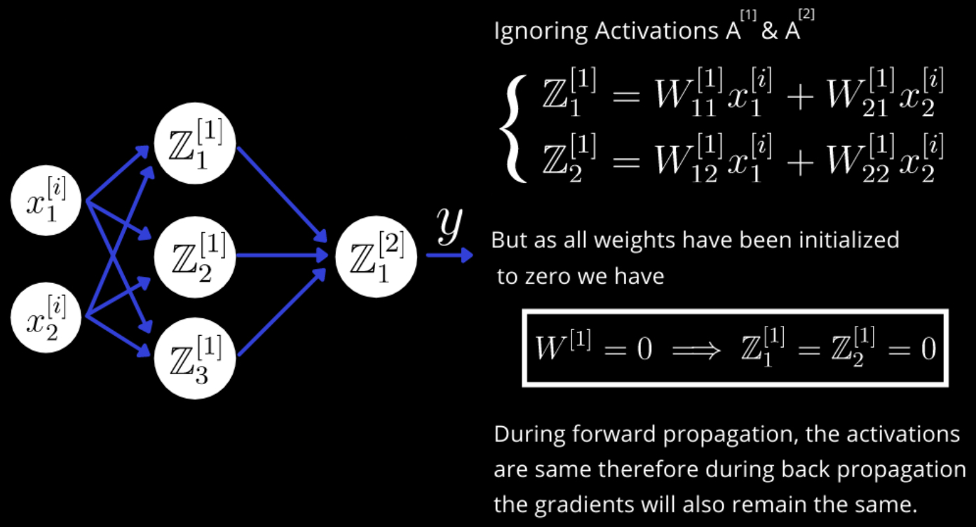
Pitfall: All Zero Initialization
-
It might seem reasonable to initialize all weights to zero, treating it as a neutral starting point. However, this creates a symmetry problem: every neuron in a layer produces the same output, receives identical gradients, and updates identically. As a result, all neurons remain the same, and the network fails to learn distinct features.
-
The following figure (source) illustrates why initializing all weights to zero fails. Neurons collapse into identical behavior, preventing learning.
Small Random Numbers
-
A common solution is to initialize weights with small random numbers, often drawn from a Gaussian or uniform distribution. This breaks symmetry, allowing neurons to develop unique feature detectors:
W = 0.01 * np.random.randn(D, H)- where
randnsamples from a zero-mean, unit-variance Gaussian. Every neuron’s weight vector is initialized randomly, pointing in different directions in input space.
- where
-
Warning: Smaller is not always better. If weights are too small, gradients become extremely weak during backpropagation, leading to vanishing updates in deep networks.
Variance Calibration and the 1/\(\sqrt{n}\) Rule
- The variance of a neuron’s output grows with the number of inputs. To stabilize outputs, each neuron’s weight variance should be scaled by the inverse of its fan-in (number of inputs):
w = np.random.randn(n) / np.sqrt(n)
Derivation sketch: For pre-activation \(s = \sum\_{i=1}^n w\_i x\_i\),
\[\begin{align} \text{Var}(s) &= \text{Var}\left(\sum_i^n w_ix_i\right) \\ &= \sum_i^n \text{Var}(w_i x_i) \\ &= \sum_i^n [E(w_i)]^2 \text{Var}(x_i) + [E(x_i)]^2 \text{Var}(w_i) + \text{Var}(x_i)\text{Var}(w_i) \\ &= \sum_i^n \text{Var}(x_i)\text{Var}(w_i) \\ &= \left( n \cdot \text{Var}(w) \right) \text{Var}(x) \end{align}\]- If inputs and weights are zero-mean and identically distributed, then for variance to remain stable we require \(\text{Var}(w) = 1/n\). Thus, weights should be sampled from a unit Gaussian and scaled by \(\sqrt{1/n}\).
Xavier (Glorot) Initialization
-
Xavier initialization balances the forward and backward pass variances:
\[W \sim U\left(-\frac{1}{\sqrt{N_{in}}}, \frac{1}{\sqrt{N_{in}}}\right)\]- where \(N\_{in}\) is the number of input neurons. This scheme works well with symmetric activations like tanh ((Glorot & Bengio, 2010)).
-
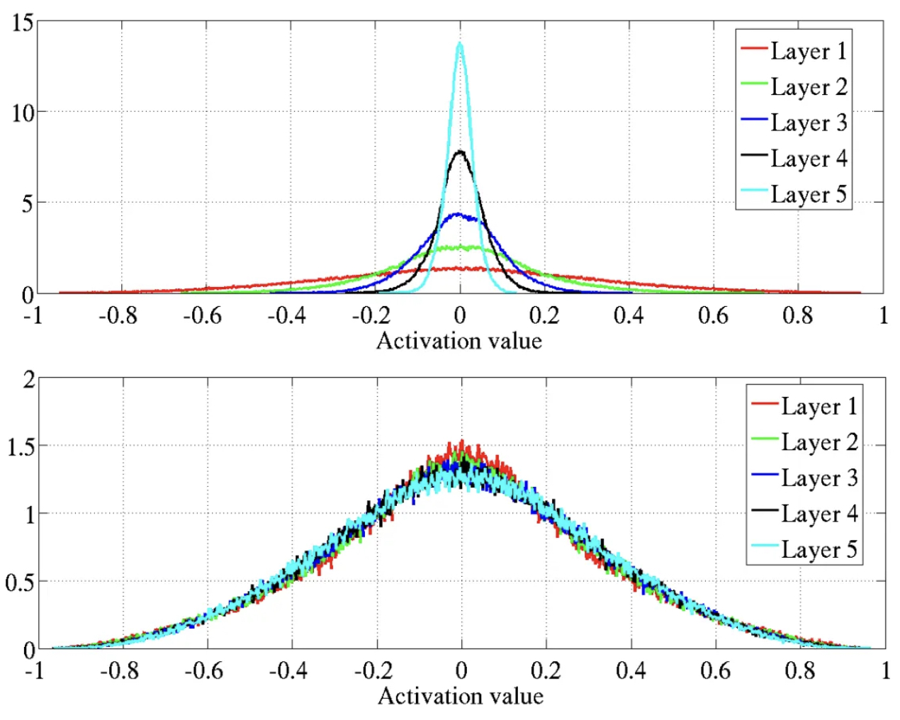
The following figure (source) demonstrates how Xavier initialization maintains stable activations across layers, avoiding vanishing or exploding gradients. Specifically, it shows the activation values normalized histograms with hyperbolic tangent activation, with standard (top) vs normalized initialization (bottom). Top: 0-peak increases for higher layers.
He Initialization for ReLU
- For ReLU activations, which zero out negative values, the variance is effectively halved. He initialization ((He et al., 2015)) compensates by scaling variance to \(2/N\_{in}\):
- This is the current best practice for deep ReLU networks.
Sparse Initialization
- An alternative strategy is sparse initialization, where most weights are set to zero, but each neuron connects to a small number of randomly chosen inputs with nonzero weights (often ~10 per neuron). This breaks symmetry while maintaining sparse representations.
Bias Initialization
- Commonly: biases are initialized to zero, since asymmetry is already broken by randomized weights.
- For ReLU units: some practitioners initialize with small positive constants (e.g., 0.01) to ensure neurons fire at the start of training. Empirical results are mixed, and zero initialization remains the norm.
In Practice
- Use He initialization (
w = np.random.randn(n) * sqrt(2.0/n)) for ReLU-based networks. - Use Xavier initialization for tanh or sigmoid networks.
- Combine initialization with batch normalization for added robustness.
- Avoid extremes: overly small weights lead to vanishing signals, while overly large weights lead to saturated activations and exploding gradients.
Additional Notes
- Sparse initialization: Some schemes initialize most weights to zero but assign small random values to a few connections per neuron.
- Bias initialization: Biases are often set to zero. For ReLU networks, small positive constants (e.g., 0.01) are sometimes used to avoid dead neurons, though results vary.
- In practice: For ReLU-based networks, the recommended default is He initialization:
w = np.random.randn(n) * np.sqrt(2.0/n)
- This choice ensures robust convergence and stable gradient flow.
Batch Normalization
-
Even with careful preprocessing and weight initialization, deep networks often suffer from internal covariate shift: the distribution of activations in each layer shifts as weights are updated during training. This forces subsequent layers to continuously readjust, slowing convergence and making training unstable.
-
To address this, (Ioffe & Szegedy, 2015) introduced Batch Normalization (BN). BN normalizes activations at each layer, ensuring they maintain a stable distribution throughout training.
-
Importantly, BN also alleviates many of the difficulties associated with weight initialization. By forcing activations within each mini-batch to approximately follow a unit Gaussian distribution, BN makes networks significantly more robust to poor initialization choices. Conceptually, it can be understood as applying data preprocessing at every layer of the network — but built directly into the model in a differentiable manner.
-
In practice, BN layers are inserted immediately after fully connected or convolutional layers and before nonlinearities. This placement stabilizes learning dynamics and accelerates convergence.
-
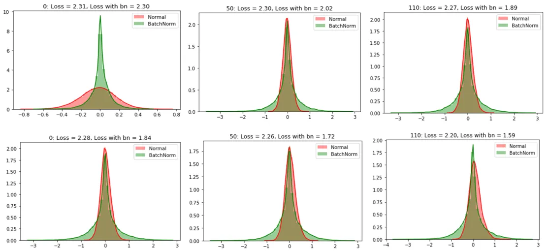
The following figure (source) shows the effect of batch normalization. From the graphs, we can conclude that the distribution of values without batch normalization has changed significantly between iterations of inputs within each epoch which means that the subsequent layers in the network without batch normalization are seeing a varying distribution of input data. Without BN, activations drift layer by layer, leading to vanishing or exploding gradients. With BN, distributions remain stable across depth, enabling efficient training.
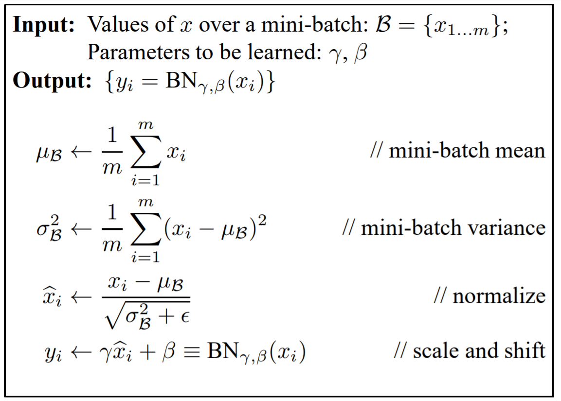
The Batch Normalization Algorithm
- Given a mini-batch of size \(m\) with activations \(x\_1, x\_2, ..., x\_m\), BN performs:
-
Compute batch statistics:
\[\mu_B = \frac{1}{m} \sum_{i=1}^m x_i, \quad \sigma_B^2 = \frac{1}{m} \sum_{i=1}^m (x_i - \mu_B)^2\] -
Normalize activations:
\[\hat{x}_i = \frac{x_i - \mu_B}{\sqrt{\sigma_B^2 + \epsilon}}\]- where \(\epsilon\) is a small constant to avoid division by zero.
-
Scale and shift:
\[y_i = \gamma \hat{x}_i + \beta\]- where \(\gamma\) and \(\beta\) are learnable parameters that allow the network to restore the original distribution if needed.
- The following figure illustrates this process step by step: activations are first centered, then normalized, and finally rescaled using learnable parameters.
Why Learn \(\gamma\) and \(\beta\)?
-
If we only normalized to zero mean and unit variance, some nonlinearities (e.g., sigmoid) would lose useful information, as inputs would collapse into a near-linear regime. By introducing \(\gamma\) and \(\beta\), BN allows the model to recover useful distributions, preventing underfitting.
-
During training, mean and variance are computed on each mini-batch. During inference, moving averages accumulated during training are used instead, ensuring consistent predictions.
Advantages of Batch Normalization
- Faster convergence: BN enables higher learning rates without instability.
- Stabilized gradients: Keeps activations within a controlled range, reducing exploding/vanishing gradients.
- Regularization effect: Adds noise through mini-batch statistics, often reducing the need for dropout.
- Reduced sensitivity to initialization: Networks with BN are significantly more robust to poor weight initialization.
- Improved generalization: BN has been shown to improve test accuracy across many architectures.
Batch Normalization in Practice
- Insert BN after linear or convolutional layers and before nonlinearities. Conceptually, it can be seen as data preprocessing at every layer — but done internally, in a differentiable way.
- During training, batch statistics are computed on each mini-batch. During inference, running averages of the mean and variance collected during training are used to ensure consistent predictions.
- BN is compatible with most optimizers (SGD, Adam, etc.), but allows higher learning rates for faster training.
- In convolutional networks, BN is often applied per feature map rather than per neuron.
Training Neural Networks: A Case Study
-
We now bring together the components introduced so far — activation functions, preprocessing, weight initialization, and batch normalization — into a complete training pipeline. This case study illustrates how these design choices interact to produce stable and efficient training.
-
At its core, training involves iteratively updating parameters to minimize a chosen loss function (e.g., cross-entropy for classification, mean squared error for regression). The efficiency and stability of this process depend critically on the strategies we have discussed.
Recap of the Training Pipeline
-
Preprocess the data:
- Subtract the mean (per-feature or per-channel for images).
- Normalize by standard deviation where appropriate.
-
Rarely: apply PCA/whitening (expensive and uncommon in modern convnets).
- The following figure illustrates a preprocessing pipeline: raw data → mean subtraction → normalization.
-
Initialize weights:
- Avoid all-zero initialization (destroys symmetry).
- Use He initialization for ReLU-based networks, or Xavier initialization for tanh/sigmoid networks.
-
Initialize biases to zero (or small positive constants for ReLU to avoid dead neurons).
- The following figure shows the problem with poor initialization. Top: all neurons collapse into identical behavior when initialized poorly. Bottom: careful initialization preserves variance and signal flow across layers.
-
Apply batch normalization:
- Insert BN layers after fully connected or convolutional layers, and before nonlinearities.
-
During training, normalize per mini-batch. During inference, use running averages.
- The following figure compares training with and without BN, highlighting how BN stabilizes distributions across depth.
-
Choose the activation function:
- Default: ReLU.
- Use variants like Leaky ReLU, PReLU, or ELU if dead neurons are an issue.
-
Consider Maxout for theoretical flexibility, but balance against computational cost.
- The following figure shows the most common nonlinearities, including sigmoid, tanh, ReLU, Leaky ReLU, ELU, and Maxout.
Putting It Together: The Training Loop
-
With these steps in place, training follows the standard loop:
- Forward pass: Propagate inputs through layers with activations and normalization.
- Loss computation: Compare predictions with labels using a loss function.
- Backward pass: Compute gradients via backpropagation.
- Parameter update: Adjust weights using an optimizer (SGD, Adam, RMSprop, etc.).
-
This process is repeated across epochs until convergence. Learning rates, batch sizes, and optimization algorithms fine-tune the performance but rely on the stable foundation set by preprocessing, initialization, and normalization.
Benefits of Careful Setup
-
Empirical results consistently show that networks with proper initialization and preprocessing converge orders of magnitude faster than poorly initialized ones. For instance:
- Without preprocessing, gradients are unbalanced, leading to divergence.
- Without careful initialization, activations vanish or explode, halting learning.
- With batch normalization, training remains stable even in very deep networks, and sensitivity to initialization is greatly reduced.
-
Together, these design principles form the backbone of modern deep learning practice, enabling architectures with hundreds of layers to be trained reliably.
Citation
If you found our work useful, please cite it as:
@article{Chadha2020TrainingNeuralNetworksI,
  title   = {Training Neural Networks I},
  author  = {Chadha, Aman},
  journal = {Distilled Notes for Stanford CS231n: Convolutional Neural Networks for Visual Recognition},
  year    = {2020},
  note    = {\url{https://aman.ai}}
}