CS231n • Recurrent Neural Networks
- Overview
- Types of RNN Input-Output Structures
- Mathematical Formulation of RNNs
- Example: Language Modeling with RNNs
- Backpropagation Through Time (BPTT)
- Truncated Backpropagation Through Time (TBPTT)
- Example: Training on Shakespeare Text
- Image Captioning with RNNs
- Advanced RNN Architectures
- Comparative Summary of RNN Architectures
- Citation
Overview
-
Recurrent Neural Networks (RNNs) represent a fundamental advancement in deep learning architectures, specifically designed for modeling sequential or temporal data. Unlike standard feedforward neural networks, which are restricted to fixed-size inputs and outputs, RNNs introduce the concept of recurrence, where the output of a previous step influences the processing of the next step. This allows them to naturally handle variable-length sequences for both inputs and outputs (Rumelhart et al., 1986).
-
The ability to process sequences makes RNNs extremely versatile across multiple domains. For instance:
- In natural language processing (NLP), RNNs can read sentences word by word, capturing the dependencies between words (Mikolov et al., 2010).
- In speech recognition, RNNs model how sounds evolve over time into words (Graves et al., 2013).
- In time-series forecasting, such as stock market prediction, they leverage historical values to predict future trends (Connor et al., 1994).
- In computer vision, they can process sequences of image frames (e.g., videos) (Donahue et al., 2015).
-
A key distinction of RNNs compared to feedforward networks lies in their use of a hidden state that persists across timesteps. This hidden state acts like a memory, storing information about what has been processed so far. By updating this state recurrently, RNNs can capture context and temporal dependencies that are critical for understanding structured sequences (Elman, 1990).
Why RNNs?
-
Traditional feedforward neural networks, such as multilayer perceptrons (MLPs) or convolutional neural networks (CNNs), are inherently stateless with respect to the order of data. They excel at tasks where inputs are independent of each other, but fail when temporal order or sequential correlation is essential.
-
Consider the following examples:
- CIFAR-10 image classification: Here, inputs are fixed-size images (32 × 32 × 3), and the network produces a fixed-size output (10 categories). Since each input is independent, order does not matter.
- Language modeling: Words form coherent meaning only when interpreted in sequence. For instance, the meaning of “bank” depends on whether the preceding words refer to “river” or “money” (Bengio et al., 2003).
- Speech recognition: Sounds unfold over time, and recognition depends on the sequence of phonemes.
- Video analysis: Frames individually convey little meaning; understanding arises from their temporal evolution.
-
Feedforward networks lack the mechanism to model such dependencies. RNNs overcome this limitation by maintaining a hidden state vector \(h_t\), which evolves over time and carries information from past timesteps.
-
This property allows RNNs to:
- Capture short-term dependencies, such as the immediate relation between adjacent words.
- Model long-term dependencies (though with difficulty in vanilla RNNs), such as subject–verb agreement across an entire sentence (Hochreiter, 1991).
- Generalize across sequences of variable lengths, unlike fixed-dimension networks.
Types of RNN Input-Output Structures
- RNNs are not limited to a single type of mapping between inputs and outputs. Their ability to handle variable-length sequences allows them to support multiple architectures depending on the task. This flexibility is what makes RNNs widely applicable across domains such as NLP, speech processing, and video analysis. Below are the standard configurations of RNN-based sequence models (Sutskever et al., 2014).
One-to-Many
- Description: A single input produces a sequence of outputs.
- Example: Image captioning, where the input is one image and the model generates a descriptive sentence (a sequence of words) (Vinyals et al., 2015).
-
Mechanism:
- The input (e.g., an image feature vector from a CNN) initializes the hidden state of the RNN.
- The RNN then generates one token (word) at a time, feeding its previous output back into itself until an end-of-sequence (EOS) token is produced.
- Key Point: Enables sequence generation from a fixed representation.
Many-to-One
- Description: A sequence of inputs produces a single output.
- Example: Sentiment classification, where the input is a sequence of words in a sentence, and the output is a single sentiment label (positive, negative, neutral) (Tang et al., 2015).
-
Mechanism:
- Each input token is processed step by step, updating the hidden state.
- At the final timestep, the last hidden state summarizes the sequence and is used to predict the output.
- Key Point: Useful when the goal is to understand a sequence as a whole and reduce it to one decision or label.
Many-to-Many
- Description: Both inputs and outputs are sequences.
- Example: Machine translation, where a sentence in one language (input sequence) is mapped into another sentence in a different language (output sequence) (Cho et al., 2014).
-
Mechanism:
- Input tokens are processed sequentially, updating the hidden state.
- At each step, the RNN may produce an output aligned with the input (e.g., frame-by-frame video classification) or after the full sequence has been encoded (e.g., sequence-to-sequence translation with alignment).
- Key Point: Allows parallel mapping of sequential inputs to sequential outputs.
Many-to-One-to-Many (Encoder-Decoder Models)
-
Description: The input sequence is first compressed into a fixed-size representation (encoder), and then another RNN (decoder) expands this into an output sequence.
-
Examples:
- Video classification frame-by-frame: Frames are encoded into a context vector, which is then decoded into per-frame predictions.
- Sequence-to-sequence NLP models: Machine translation (English \(\rightarrow\) French) where the encoder processes the source sentence and the decoder generates the target sentence (Sutskever et al., 2014).
-
Mechanism:
- Encoder: Reads the entire input sequence and encodes it into a single hidden representation (context vector).
- Decoder: Starts from this representation and generates the output sequence step by step.
-
Key Point: The foundation of seq2seq models, widely used in NLP and later enhanced with attention mechanisms (Bahdanau et al., 2015).
-
The following figure illustrates how RNNs enable variable-length input and output modeling.

- The following figure presents the computation graphs for different types of models: one-to-many, many-to-one, many-to-many, and encoder-decoder variants.


Mathematical Formulation of RNNs
- At the heart of Recurrent Neural Networks (RNNs) lies the concept of hidden state dynamics, which enable the model to capture temporal dependencies. Unlike feedforward networks that map input vectors directly to outputs, RNNs introduce recurrence, where outputs at one timestep depend not only on the current input but also on information carried over from previous timesteps. This section formalizes the mathematical structure of RNNs (Elman, 1990).
- This mathematical framework is the foundation for all recurrent architectures. It sets the stage for understanding more complex mechanisms such as Backpropagation Through Time (BPTT), which trains RNNs by propagating errors across timesteps (Werbos, 1990).
Recursive Update Rule
The hidden state evolves through time based on both the new input and the previous hidden state. Formally:
\[h_t = f(h_{t-1}, x_t; W)\]-
where:
- \(h_t\): hidden state at timestep \(t\), encoding all information seen so far
- \(h_{t-1}\): hidden state from the previous timestep
- \(x_t\): input vector at timestep \(t\)
- \(W\): set of learnable weight matrices and bias terms
- \(f\): nonlinear function (activation), such as tanh, ReLU, or sigmoid
-
Interpretation:
- The recursive nature allows the network to “remember” prior inputs, enabling it to model sequential data.
- The hidden state serves as a summary of past information relevant for current predictions.
Vanilla RNN Update
-
A common instantiation of the update rule is the vanilla RNN, which uses the hyperbolic tangent nonlinearity (Rumelhart et al., 1986):
\[h_t = \tanh(W_{hh} h_{t-1} + W_{xh} x_t + b_h)\]-
where:
- \(W_{hh}\): weight matrix for the recurrent connection (previous hidden state \(\rightarrow\) current hidden state)
- \(W_{xh}\): weight matrix for the input connection (input \(\rightarrow\) hidden state)
- \(b_h\): bias vector
- \(\tanh(\cdot)\): ensures bounded activations in the range \([-1, 1]\), helping stabilize gradients compared to raw linear updates
-
-
Interpretation:
- The update combines the influence of the previous hidden state and the current input, then passes it through a nonlinearity to allow complex feature representations.
- This recurrent formulation makes the RNN behave like a dynamical system evolving over time.
Output Computation
-
The hidden state is then used to compute an output:
\[y_t = W_{hy} h_t + b_y\]- where:
- \(y_t\): predicted output at timestep \(t\)
- \(W_{hy}\): weight matrix mapping hidden state \(\rightarrow\) output
- \(b_y\): bias vector
-
In practice:
- For classification tasks, \(y_t\) is passed through a softmax layer to yield probabilities over classes.
- For regression tasks, \(y_t\) may be a continuous-valued prediction.
Sequence-Level Perspective
-
By unrolling the RNN over \(T\) timesteps, we can write:
- Inputs: \(x_1, x_2, \dots, x_T\)
- Hidden states: \(h_1, h_2, \dots, h_T\)
- Outputs: \(y_1, y_2, \dots, y_T\)
-
This creates a computation graph where each timestep reuses the same parameters \(W_{xh}, W_{hh}, W_{hy}\), making the model parameter-efficient regardless of sequence length.
Intuition: Memory through Hidden States
- The hidden state \(h_t\) can be thought of as the network’s memory.
- For short sequences, vanilla RNNs perform well because they can store useful context for nearby steps.
- For longer sequences, however, problems arise: gradients may vanish or explode during training, leading to difficulty in learning long-range dependencies. (This limitation is later addressed by LSTMs and GRUs (Hochreiter & Schmidhuber, 1997; Cho et al., 2014)).
Example: Language Modeling with RNNs
- One of the most common and illustrative applications of RNNs is language modeling, where the task is to predict the next word or character given a sequence of previous inputs. This problem highlights the ability of RNNs to capture temporal dependencies in sequential data (Mikolov et al., 2010).
- This example demonstrates how RNNs can predict sequential data and generate coherent outputs, forming the basis for more advanced architectures like LSTMs, GRUs, and Transformers in natural language processing (Bengio et al., 2003).
Goal of Language Modeling
-
Given a sequence of tokens \(x_1, x_2, \dots, x_T\), the model learns to estimate the conditional probability distribution:
\[P(x_t | x_1, x_2, \dots, x_{t-1})\] -
The network processes the input tokens step by step and uses its hidden state to accumulate context.
-
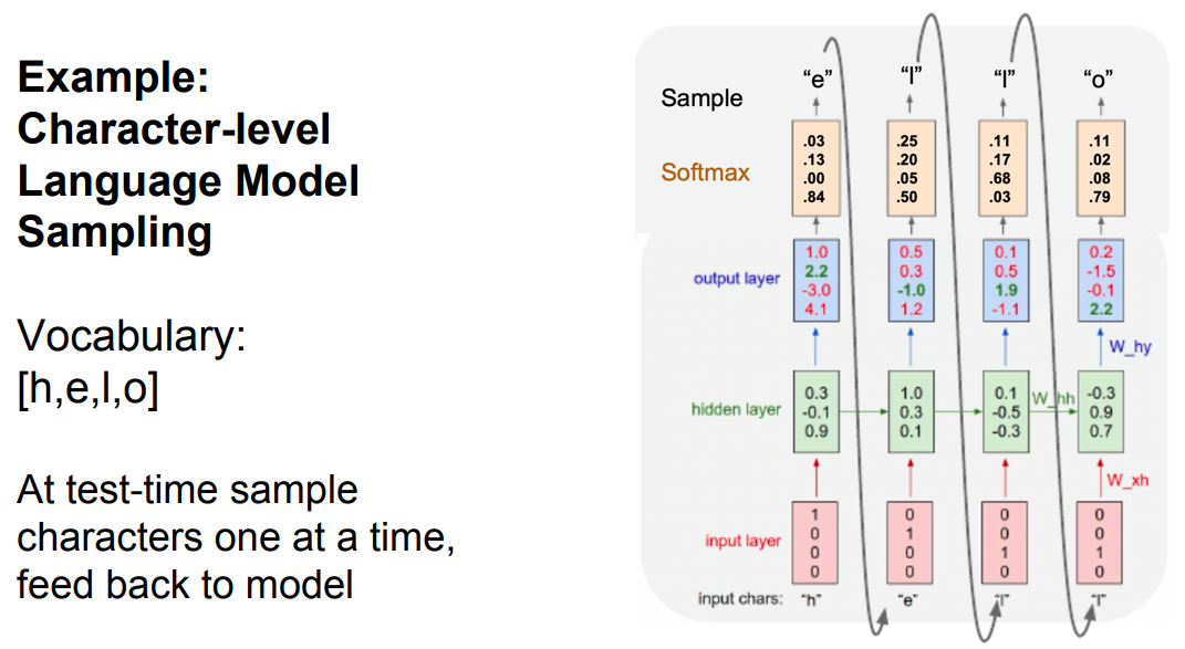
At each step, the model outputs a probability distribution over the vocabulary, from which the next token can be sampled or chosen.
Input Representation
-
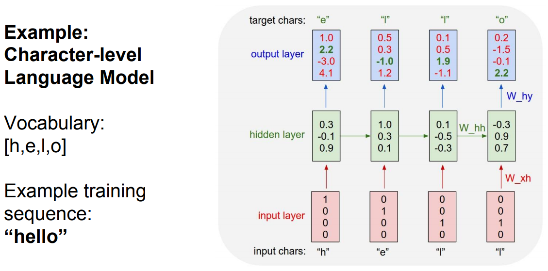
Since neural networks operate on numerical data, textual inputs need to be converted into vectors:
-
One-hot encoding:
- Each word or character in the vocabulary is represented as a vector of size equal to the vocabulary size \(V\).
- For example, with vocabulary [h, e, l, o], the word “h” would be encoded as \([1, 0, 0, 0]\), “e” as \([0, 1, 0, 0]\), etc.
-
Embedding vectors (in practice):
- Instead of sparse one-hot vectors, we often use embeddings (dense vectors of lower dimension) that capture semantic similarity between tokens (Mikolov et al., 2013).
- E.g., “king” and “queen” will have closer embeddings compared to “king” and “banana”.
-
Hidden State Updates
At each timestep \(t\):
-
The model takes the current token representation \(x_t\).
-
Updates the hidden state using the recurrence relation:
\[h_t = \tanh(W_{hh} h_{t-1} + W_{xh} x_t + b_h)\] -
This ensures that the hidden state \(h_t\) encodes not just the current input but also the context of all previous inputs.
Output Prediction
-
The hidden state \(h_t\) is mapped to an output vector:
\[y_t = W_{hy} h_t + b_y\] -
The softmax function is then applied:
\[\hat{p}_t = \text{softmax}(y_t)\] -
Here, \(\hat{p}_t\) represents a probability distribution over all possible tokens in the vocabulary.
-
The next character/word is chosen either by:
- Argmax (choosing the most probable token).
- Sampling (randomly selecting according to the probability distribution).
Training
- During training, the model is provided with sequences where the true next token is known.
- The loss function is typically the cross-entropy loss between the predicted distribution \(\hat{p}_t\) and the true token (represented as a one-hot vector).
- Errors are backpropagated through the network (via Backpropagation Through Time, BPTT) (Werbos, 1990).
Inference and Text Generation
-
Once trained, the model can generate text by:
- Starting with a seed sequence (e.g., “The”).
- Predicting the next token distribution.
- Sampling the next token and feeding it back into the RNN.
- Repeating the process until an end condition is met (e.g., EOS token or max length).
-
Over time, the generated text starts resembling the structure and style of the training corpus (e.g., Shakespeare’s plays) (Karpathy, 2015).
-
The following figure shows how a trained language model samples the next character from a probability distribution.
- The following figure depicts the structure of a vanilla RNN: one-hot encoded input \(\rightarrow\) hidden state updates \(\rightarrow\) output predictions.
Backpropagation Through Time (BPTT)
-
Training Recurrent Neural Networks (RNNs) is more complex than training feedforward neural networks due to their temporal recurrence. In feedforward networks, gradients are propagated layer by layer. In RNNs, however, gradients must flow not just across layers but also across time steps. This specialized procedure is known as Backpropagation Through Time (BPTT) (Werbos, 1990).
-
In essence, BPTT is what makes RNN training possible but also highlights the core difficulties of vanilla RNNs, which motivated the development of more advanced architectures.
Key Idea of BPTT
-
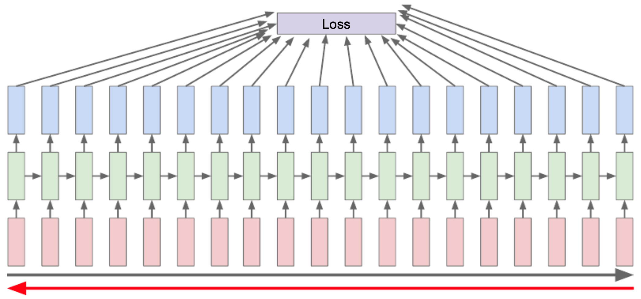
When an RNN is unrolled over \(T\) timesteps, it effectively becomes a deep feedforward network of depth \(T\), where each layer corresponds to one timestep and shares the same parameters \(W\) (Rumelhart et al., 1986).
-
Forward pass:
- Inputs \(x_1, x_2, \dots, x_T\) are processed sequentially to produce hidden states \(h_1, h_2, \dots, h_T\) and outputs \(y_1, y_2, \dots, y_T\).
-
Loss computation:
- A loss function \(L\) is defined over the outputs (e.g., cross-entropy for language modeling).
-
The total loss is usually the sum of per-timestep losses:
\[L = \sum_{t=1}^T L_t(y_t, \hat{y}_t)\]
-
Backward pass:
- Gradients of the loss are propagated backward in time through the unrolled network, updating the shared parameters.
Gradient Flow
- The gradient of the loss with respect to parameters depends on the chain of derivatives over all timesteps. For example, the derivative of the loss at timestep \(T\) with respect to parameters \(W\) is:
- Since \(h_t = f(W_{hh} h_{t-1} + W_{xh} x_t)\), the gradient at timestep \(t\) also depends recursively on gradients from all earlier timesteps.
- This recursive dependency is the essence of BPTT—it backpropagates errors not just through layers but also through the timeline of the sequence.
Challenges of BPTT
- While conceptually straightforward, BPTT faces two major practical challenges:
Computational Expense
- For long sequences, the unrolled RNN can be extremely deep (e.g., thousands of timesteps).
- Backpropagating through all steps requires large memory to store intermediate activations and long computation time.
- Example: Training on the entire Wikipedia corpus in one pass would be infeasible (Mikolov et al., 2012).
Vanishing and Exploding Gradients
-
During backpropagation, gradients are repeatedly multiplied by the recurrent weight matrix \(W_{hh}\) (Bengio et al., 1994).
-
If the eigenvalues of \(W_{hh}\) are less than 1, gradients shrink exponentially \(\rightarrow\) vanishing gradients.
-
If eigenvalues are greater than 1, gradients grow exponentially \(\rightarrow\) exploding gradients.
-
Mathematically, the gradient involves terms like:
-
This product of Jacobians can easily diminish to nearly zero or blow up to infinity as \(k\) increases.
- Vanishing gradients: Prevent the model from learning long-term dependencies (distant timesteps barely affect learning).
- Exploding gradients: Cause numerical instability, making optimization diverge.
Practical Workarounds
-
To handle these challenges, practitioners often use:
- Gradient clipping: Rescales gradients when they exceed a threshold to prevent explosion (Pascanu et al., 2013).
- Careful initialization: Choosing weight initialization schemes that reduce the risk of vanishing/exploding.
- Advanced RNNs (LSTM, GRU): Use gating mechanisms to preserve gradients over longer contexts (Hochreiter & Schmidhuber, 1997; Cho et al., 2014).
- Truncated BPTT: Limits the number of timesteps over which gradients are backpropagated (discussed next).
-
The following figure illustrates the idea of calculating the loss at the end of the time series and propagating gradients backward through time.
Truncated Backpropagation Through Time (TBPTT)
- While Backpropagation Through Time (BPTT) provides the theoretical foundation for training RNNs, applying it to long sequences quickly becomes computationally infeasible. To address this, practitioners use Truncated Backpropagation Through Time (TBPTT), a practical approximation that allows efficient training while still capturing useful temporal dependencies (Williams & Peng, 1990).
- In summary, TBPTT is the practical training strategy for RNNs: it balances efficiency with performance by focusing gradient updates on a manageable temporal window, while still allowing the hidden state to evolve across the full sequence.
Motivation for TBPTT
- Full BPTT requires unrolling the RNN across the entire sequence, computing forward and backward passes for every timestep.
-
For very long sequences (e.g., books, Wikipedia articles, video streams), this is:
- Too slow (time complexity grows with sequence length).
- Too memory-intensive (hidden states and activations from all steps must be stored).
- Moreover, due to vanishing/exploding gradients, propagating error signals across hundreds or thousands of timesteps rarely provides useful information (Bengio et al., 1994).
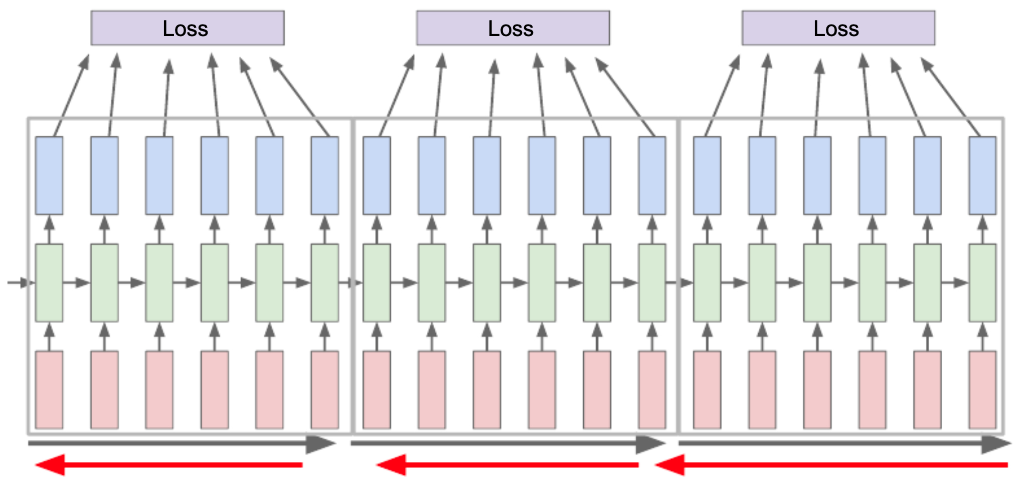
Key Idea: Instead of backpropagating through the entire sequence, we only backpropagate through a fixed-length window of timesteps (say 50–200 steps).
How TBPTT Works
- The RNN still processes the entire sequence forward to compute hidden states for each timestep.
-
However, during backpropagation, gradients are only propagated backward through a fixed number of past steps.
- For example, if the truncation length is \(k = 100\), then when computing gradients at timestep \(t\), we only consider dependencies up to \(t-100\).
- Dependencies beyond 100 steps are ignored.
Formally, this means:
- Instead of unrolling the RNN across all timesteps \(T\),
- We unroll only across chunks of size \(k\), and compute gradients locally.
Analogy with Mini-Batch Gradient Descent
-
Full BPTT vs. TBPTT is similar to batch gradient descent vs. mini-batch gradient descent:
- Full BPTT = computing gradients on the entire sequence (expensive but exact).
- TBPTT = computing gradients on subsequences (approximate but efficient).
-
Just as mini-batches speed up training for large datasets, TBPTT makes training feasible for long sequences.
Benefits of TBPTT
- Efficiency: Requires far less memory and computation than full BPTT.
- Scalability: Makes it possible to train RNNs on large datasets like Wikipedia or long speech/audio sequences (Mikolov et al., 2012).
- Stability: Reduces the risk of gradient instability across excessively long horizons.
- Good enough for practice: In many real-world tasks, dependencies beyond 100–200 steps are either not critical or can be modeled indirectly via higher-level structures (e.g., LSTMs, attention).
Limitations of TBPTT
-
Information loss: Dependencies beyond the truncation window cannot be captured directly.
-
Hyperparameter sensitivity: The truncation length \(k\) must be carefully chosen; too small and long dependencies are ignored, too large and computation becomes costly again.
-
Still sequential: Even with truncation, TBPTT does not fully parallelize training across long sequences.
-
The following figure illustrates truncated BPTT, where the sequence is divided into manageable chunks, similar to how mini-batch gradient descent works compared to full-batch.
Example: Training on Shakespeare Text
- A well-known demonstration of RNNs in action is character-level language modeling on Shakespeare’s works. This example highlights both the learning process of RNNs and their ability to generate text that resembles natural language. The experiment became widely popular after Karpathy’s blog post (2015).
- This example serves as both an engaging demonstration of RNN capabilities and a motivation for more advanced architectures (LSTMs, GRUs, attention) that address vanilla RNN limitations in handling long-range dependencies.
Task Setup
-
Input: A long text corpus (Shakespeare’s plays) is broken down into sequences of characters.
-
Vocabulary: Consists of all unique characters (letters, digits, punctuation, whitespace). For Shakespeare, this is around 60–100 characters.
-
Objective: At each timestep, predict the next character given all previous characters.
-
Formally, given a sequence \((x_1, x_2, \dots, x_T)\), the model learns:
Training Process
- Each character is one-hot encoded (or embedded into a dense vector).
- The RNN processes the characters one by one, updating its hidden state.
- At each step, the output is a probability distribution over the vocabulary (via softmax).
- The model is trained using cross-entropy loss against the true next character.
- Training uses TBPTT to manage sequence length efficiently (Williams & Peng, 1990).
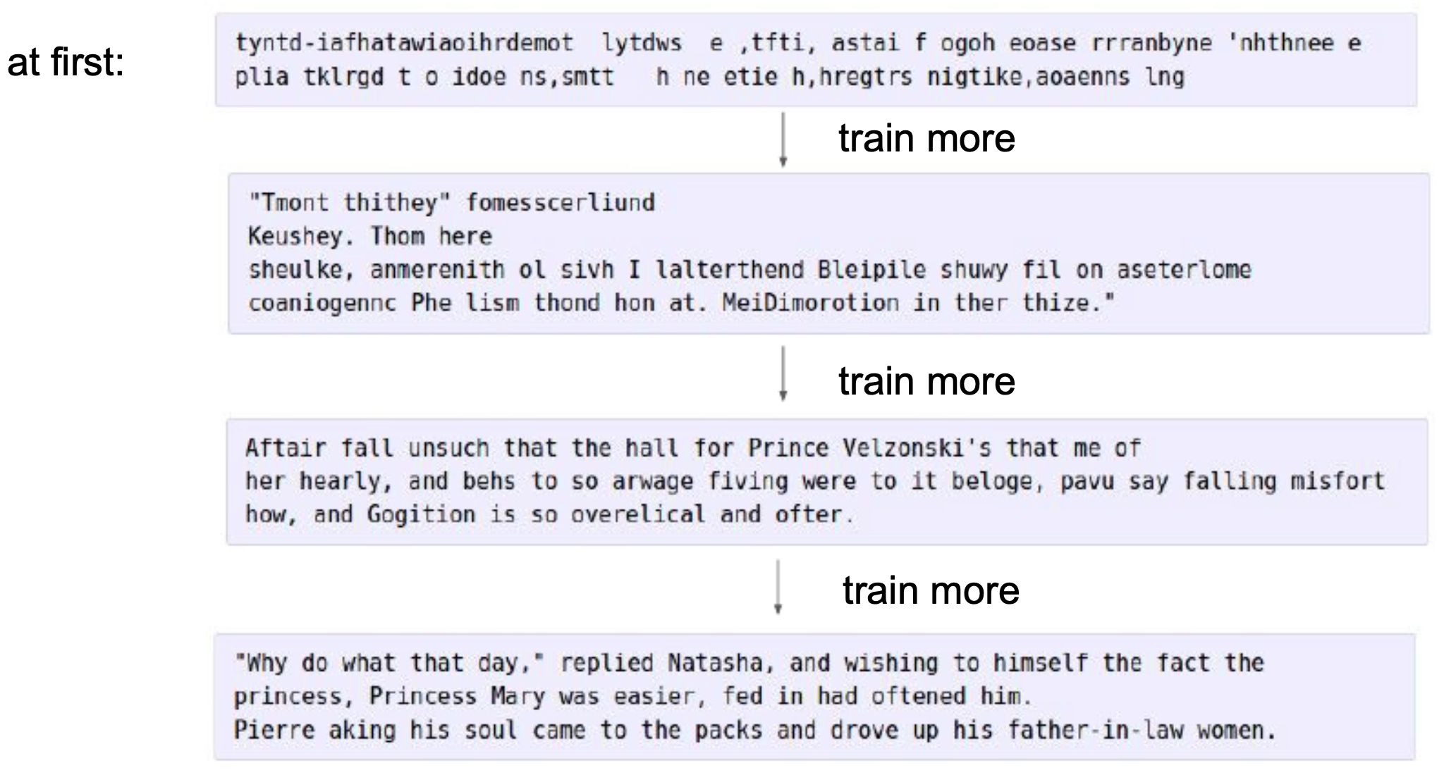
Evolution of Learning
-
The fascinating part of this experiment is observing how the generated text improves over training epochs:
-
Early Stages (Random Output)
- Initially, the RNN generates gibberish: random combinations of letters, punctuation, and spacing.
- Example:
aeklm qzzp... - Reason: The network weights are untrained, so predictions are essentially random.
-
Intermediate Stages (Local Patterns)
-
The model starts learning local statistical regularities, such as:
- Common English letter pairs (“th”, “he”).
- Punctuation patterns (quotes, parentheses).
- Word-like structures (though not meaningful).
- Example:
the frand wha - Shows evidence of the RNN memorizing short-term dependencies.
-
-
Later Stages (Shakespeare-like Output)
-
With sufficient training, the model captures grammar-like structures and stylistic features:
- Proper spacing, capitalization, and punctuation.
- Realistic sentence-like fragments.
- Mimics Shakespeare’s vocabulary and rhythm, though not always semantically correct.
-
Example:
ROMEO:
What light through yonder window breaks?
JULIET:
O gentle night!
-
- Even though the content is not truly meaningful, the structure convincingly resembles Shakespeare.
-
Key Insights
-
Sequential Dependence: The experiment shows that RNNs can capture character-level dependencies, producing coherent text structure.
-
Limitations of Vanilla RNNs: While they learn local dependencies well, modeling very long-range dependencies (like plot consistency across paragraphs) remains difficult due to vanishing gradients (Bengio et al., 1994).
-
Demonstration of Style Transfer: RNNs can replicate stylistic features of the training corpus (punctuation style, capitalization, rhythm of language).
-
The following figure shows outputs at different training phases for a Shakespeare-trained RNN.
Inspecting the Hidden State
- The hidden state in an RNN serves as its internal memory, evolving step by step as inputs are processed. By examining hidden states during training or inference, we gain insight into what the model has learned and how confident it is in its predictions. This interpretability aspect is crucial in understanding both the strengths and limitations of RNNs (Elman, 1990).
- In essence, inspecting hidden states reveals how RNNs encode memory and express uncertainty, giving us interpretability that complements their generative power.
Role of the Hidden State
-
At timestep \(t\), the hidden state \(h_t\) encodes:
- The current input \(x_t\).
- The cumulative context from all prior inputs \((x_1, \dots, x_{t-1})\).
-
In language modeling:
- \(h_t\) represents a summary of the text sequence seen so far.
- This summary is dynamic—shifting as new characters or words are processed.
Confidence in Predictions
-
When the RNN generates an output distribution over the vocabulary:
-
Confident Predictions:
- Occur when the network strongly favors one character/word over all others.
- Example: After seeing “Shakespear”, the model is very likely to predict “e” next.
- The softmax output shows one high probability value (e.g., 0.95) and very low values for others.
-
Uncertain Predictions:
- Arise when multiple characters are plausible.
- Example: After “th”, the next character could be “e” (most likely) or “a” (in some cases).
- The softmax output is more spread out (e.g., 0.45 for “e”, 0.40 for “a”, others small).
-
By analyzing hidden states and corresponding output distributions, we can directly observe how certain or uncertain the model is at each step.
Visualization of Confidence
-
Researchers often use visualization tools to highlight confidence:
- Color coding: Characters predicted with high confidence are shown in one color (e.g., red), while uncertain predictions are shown in another (e.g., blue).
- This provides an intuitive way to see where the model “knows what it’s doing” versus where it is guessing (Karpathy, 2015).
Practical Implications
-
Error Analysis: By inspecting hidden states, we can identify where the model struggles (e.g., uncommon word transitions, ambiguous contexts).
-
Interpretability: Provides a window into how RNNs process sequences internally—helpful for debugging and improving models (Lipton, 2016).
-
Generative Behavior: Explains why generated text sometimes shifts between coherent and incoherent—uncertainty at one step can propagate downstream.
-
The following figure highlights characters where the model is confident (in red) versus uncertain (in blue).
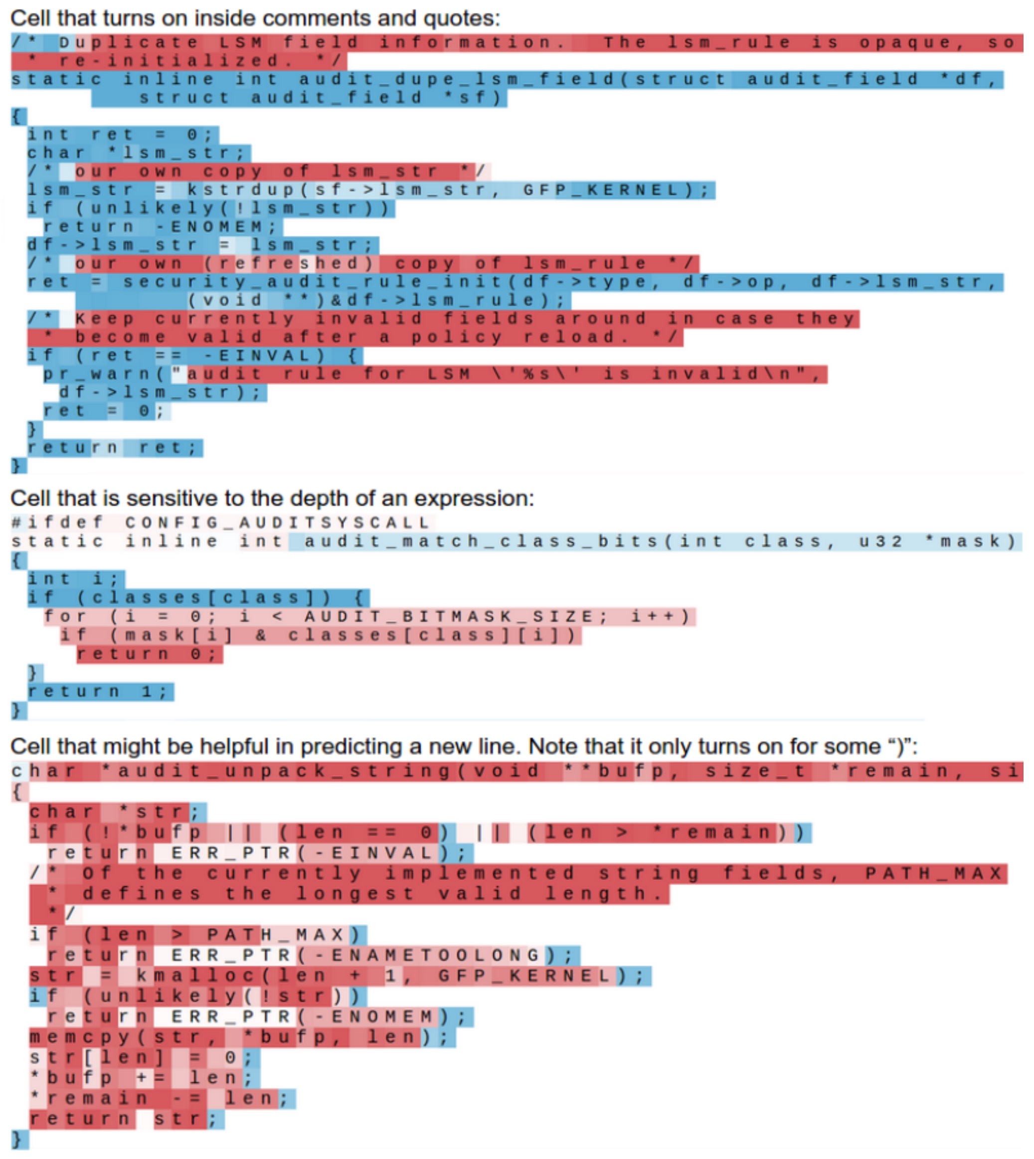
Image Captioning with RNNs
- One of the most influential applications of RNNs is image captioning, where the goal is to generate a natural language description for a given image. This task elegantly combines computer vision (understanding the image) with natural language processing (generating a descriptive sentence).
- In summary, RNN-based image captioning was a milestone in multimodal AI, showcasing how deep learning can combine vision and language. It also paved the way for modern vision-language architectures (e.g., CLIP, BLIP, Flamingo, and GPT-4V). Key early works include Mao et al., 2015, Vinyals et al., 2015, and Karpathy & Fei-Fei, 2015.
Problem Setup
- Input: An image (raw pixels).
- Output: A sequence of words forming a descriptive caption.
- Challenge: Unlike classification tasks with fixed outputs, captions are variable-length sequences that require sequential modeling of natural language.
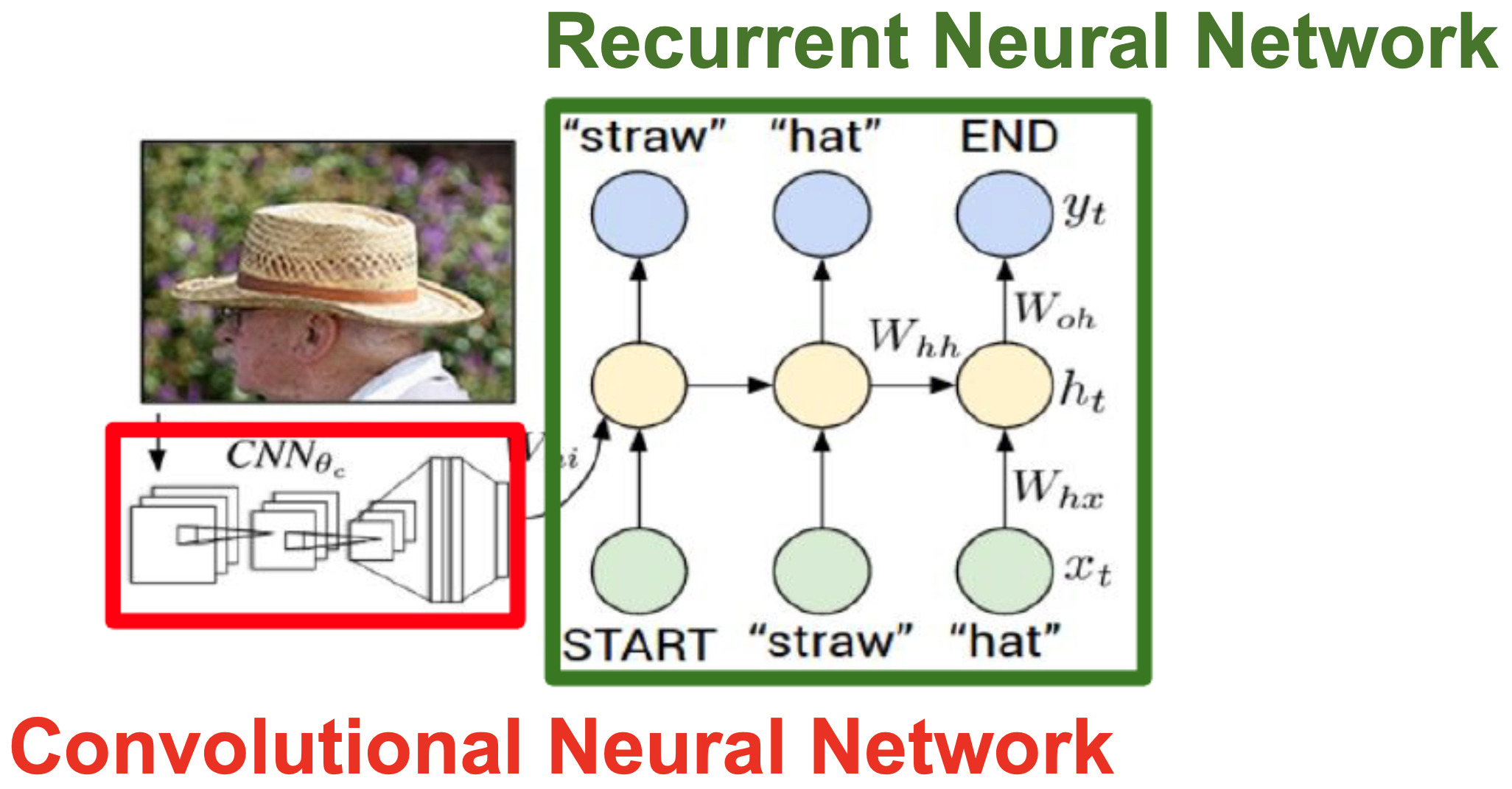
General Architecture
-
The most common framework follows a CNN \(\rightarrow\) RNN pipeline:
-
Feature Extraction with CNN
- The input image is passed through a convolutional neural network (CNN) such as ResNet, VGG, or Inception (Krizhevsky et al., 2012).
- Instead of using the final classification layer, we extract features from one of the later layers.
- These features encode high-level semantic information (objects, textures, context) from the image.
-
Sequence Generation with RNN
- The extracted feature vector is fed into an RNN (usually LSTM/GRU), acting as the initial hidden state.
-
At each timestep, the RNN generates one word conditioned on:
- The image embedding.
- The previously generated words.
- The output distribution is computed with a softmax layer over the vocabulary.
-
Training Strategies
-
End-to-End Training:
- The CNN and RNN are trained jointly.
- Gradients flow from the captioning loss back through the RNN into the CNN.
- This allows the CNN to learn features that are directly useful for captioning, not just classification.
-
Loss Function:
-
Typically, cross-entropy loss is used at each timestep:
\[L = - \sum_{t=1}^T \log P(y_t | y_{1:t-1}, \text{Image})\]
-
-
Teacher Forcing (Williams & Zipser, 1989):
- During training, instead of feeding the model’s prediction at timestep \(t-1\) into the RNN, we feed the ground-truth word.
- This speeds up convergence and stabilizes training.
-
Regularization:
- Dropout is often applied to prevent overfitting.
- Data augmentation on images helps improve generalization.
Inference (Caption Generation)
-
At test time, we cannot use teacher forcing. Instead, we must rely on the model’s own predictions:
- Greedy Decoding: Choose the most probable word at each timestep (argmax of softmax).
- Sampling: Randomly sample words from the predicted probability distribution.
- Beam Search (most popular): Explore multiple possible caption paths simultaneously, keeping the top \(k\) candidates at each timestep, and selecting the sequence with the highest overall probability (Sutskever et al., 2014).
-
Beam search significantly improves caption quality by balancing between local word choices and global sequence coherence.
Advantages of RNN-based Captioning
- Sequential Coherence: Captures grammar and syntax in natural language.
- Visual-Linguistic Fusion: CNN features provide semantic grounding, while RNNs generate structured language.
- Flexibility: Can handle captions of arbitrary length.
Extensions and Improvements
-
Attention Mechanisms: Instead of conditioning only on a single CNN feature vector, attention allows the RNN to focus on different spatial regions of the image at each timestep (Xu et al., 2015).
-
Reinforcement Learning: Optimizing captions for sequence-level metrics like BLEU, METEOR, or CIDEr rather than just next-word accuracy (Rennie et al., 2017).
-
Transformers: Replacing RNNs with transformer decoders (e.g., in modern models like Show, Attend and Tell, and later Vision-Language Transformers) (Vaswani et al., 2017).
-
The following figure illustrates the image captioning network: an image is passed through a CNN, and its semantic representation is fed into a one-to-many RNN to produce a caption.
Advanced RNN Architectures
- While vanilla RNNs provide the foundational framework for sequence modeling, they suffer from significant drawbacks, most notably the vanishing and exploding gradient problem. These limitations make it difficult for vanilla RNNs to capture long-term dependencies in sequences (e.g., remembering the subject of a sentence when predicting a verb many words later). To address these shortcomings, several advanced RNN architectures have been proposed: Long Short-Term Memory (LSTM), Gated Recurrent Units (GRU), and Attention-based RNNs.
Long Short-Term Memory (LSTM)
-
Motivation: Introduced by Hochreiter & Schmidhuber (1997), LSTMs explicitly address the vanishing gradient problem by introducing gates that regulate the flow of information through the network.
-
LSTMs maintain two states:
- Hidden state (\(h\_t\)): short-term representation.
- Cell state (\(C\_t\)): long-term memory, enabling preservation of information over many timesteps.
-
Equations: At each timestep \(t\):
- Forget gate (what to discard):
- Input gate (what new info to add):
- Cell state update:
- Output gate (what to reveal):
- where, \(\sigma\) is the sigmoid function, and \(\odot\) denotes element-wise multiplication.
-
Benefits:
- Can preserve long-term dependencies effectively.
- Mitigates vanishing gradients with its controlled gating mechanism.
- Achieves state-of-the-art performance on tasks like machine translation, speech recognition, and handwriting generation (Graves, 2013).
Gated Recurrent Unit (GRU)
-
Motivation: Introduced by Cho et al. (2014), GRUs are a simplified version of LSTMs, designed to achieve similar benefits with fewer parameters.
-
Unlike LSTMs, GRUs do not maintain a separate cell state. Instead, they merge the hidden and cell states into a single vector.
-
They use two gates:
- Update gate (\(z_t\)): controls how much of the past to keep.
- Reset gate (\(r_t\)): controls how much of the past to forget.
-
Equations:
- Update gate:
- Reset gate:
- Candidate hidden state:
- Final hidden state:
-
Benefits:
- Fewer parameters than LSTMs \(\rightarrow\) faster training.
- Performs comparably to LSTMs on many sequence tasks.
- Particularly effective in tasks like speech recognition, text classification, and conversational modeling (Chung et al., 2014).
Attention Mechanisms in RNNs
-
Motivation: Even with LSTMs and GRUs, encoding an entire input sequence into a single fixed-length vector is a bottleneck, especially for very long sequences (e.g., paragraph-level machine translation).
-
Core Idea: Instead of relying only on the final hidden state, attention allows the decoder to dynamically focus on relevant parts of the input sequence at each output step (Bahdanau et al., 2015).
-
Mathematics:
- Compute attention weights for each encoder hidden state:
-
\(s_{t-1}\): decoder state at time \(t-1\).
-
\(h_i\): encoder hidden state at position \(i\).
- Compute context vector:
- Use \(c_t\) along with \(s_{t-1}\) to predict the next output.
-
Benefits:
- Handles long sequences more effectively.
- Provides interpretability—we can visualize which parts of the input the model focuses on.
- Significantly improves tasks like neural machine translation, image captioning, and document summarization.
From Attention to Transformers
- Attention mechanisms in RNNs laid the groundwork for Transformers (Vaswani et al., 2017).
- Transformers remove recurrence entirely, replacing it with self-attention, enabling full parallelization and better long-range modeling.
- This shift led to modern architectures such as BERT, GPT, and Vision-Language Transformers.
Summary of Advanced RNNs
- LSTMs: Maintain long-term memory via gates and cell state; highly expressive but computationally heavier.
- GRUs: Simplified LSTMs with fewer gates and faster training; effective for many tasks.
- Attention: Removes the fixed-length bottleneck, allowing selective focus on relevant inputs; the precursor to Transformers.
Comparative Summary of RNN Architectures
- This comparative summary shows the evolution of sequence modeling architectures—from simple recurrent updates in Vanilla RNNs to sophisticated attention-driven models that inspired today’s large-scale Transformers. It highlights the core idea, mechanisms, strengths, limitations, and typical applications of each architecture.
Key Comparison Table
| Architecture | Core Idea | Equations / Mechanisms | Strengths | Limitations | Typical Applications |
|---|---|---|---|---|---|
| Vanilla RNN ([Elman, 1990](https://crl.ucsd.edu/~elman/Papers/fsit.pdf)) | Hidden state updated recursively across timesteps to capture sequential dependencies. | \(h_t = \tanh(W_{hh} h_{t-1} + W_{xh} x_t)\) | Simple and efficient for short sequences. Provides the conceptual foundation for advanced RNNs. | Suffers from vanishing/exploding gradients ([Bengio et al., 1994](https://www.iro.umontreal.ca/~bengioy/papers/trnn94.pdf)). | Language modeling (short sequences), basic sequence classification. |
| LSTM ([Hochreiter & Schmidhuber, 1997](https://www.bioinf.jku.at/publications/older/2604.pdf)) | Introduces cell state with input, forget, and output gates to manage long-term memory. | \(C_t = f_t \odot C_{t-1} + i_t \odot \tilde{C}_t,\quad h_t = o_t \odot \tanh(C_t)\) | Captures long-range dependencies. Mitigates vanishing gradient problem. Highly expressive. | Computationally heavier with more parameters. Slower training. | Machine translation, speech recognition, handwriting generation ([Graves, 2013](https://arxiv.org/abs/1308.0850)). |
| GRU ([Cho et al., 2014](https://arxiv.org/abs/1406.1078)) | Simplified LSTM with update and reset gates, merging hidden and cell states into one representation. | \(h_t = (1 - z_t) \odot h_{t-1} + z_t \odot \tilde{h}_t\) | Fewer parameters $$\rightarrow$$ faster training. Performs comparably to LSTMs on many tasks. | Slightly less expressive than LSTMs. May underperform on very long dependencies. | Text classification, conversational models, music generation ([Chung et al., 2014](https://arxiv.org/abs/1412.3555)). |
| Attention-based RNN ([Bahdanau et al., 2015](https://arxiv.org/abs/1409.0473)) | Dynamically focuses on relevant encoder states instead of compressing into a fixed vector. | \(c_t = \sum_i \alpha_{t,i} h_i, \quad \alpha_{t,i} = \text{softmax}(\text{score}(s_{t-1}, h_i))\) | Handles long sequences effectively. Provides interpretability. Removes fixed-length bottleneck. | More computationally expensive. Acts as a precursor to Transformers. | Neural machine translation, image captioning ([Xu et al., 2015](https://arxiv.org/abs/1502.03044)), document summarization. |
Takeaways
- Vanilla RNNs: Useful for intuition and short sequences but impractical for complex tasks.
- LSTMs: Powerful and expressive, widely adopted before Transformers became dominant.
- GRUs: Lightweight alternative to LSTMs, balancing speed and performance.
- Attention Mechanisms: Revolutionized sequence modeling by allowing selective focus, paving the way for Transformer architectures (Vaswani et al., 2017).
Citation
If you found our work useful, please cite it as:
@article{Chadha2020RecurrentNeuralNetworks,
  title   = {Recurrent Neural Networks},
  author  = {Chadha, Aman},
  journal = {Distilled Notes for Stanford CS231n: Convolutional Neural Networks for Visual Recognition},
  year    = {2020},
  note    = {\url{https://aman.ai}}
}