CS231n • Deep Reinforcement Learning
- Review: Supervised and Unsupervised Learning
- Reinforcement Learnings: The Basics
- What is Reinforcement Learning?
- Markov Decision Processes (MDPs)
- Q-Learning
- Further Reading
- Citation
Review: Supervised and Unsupervised Learning
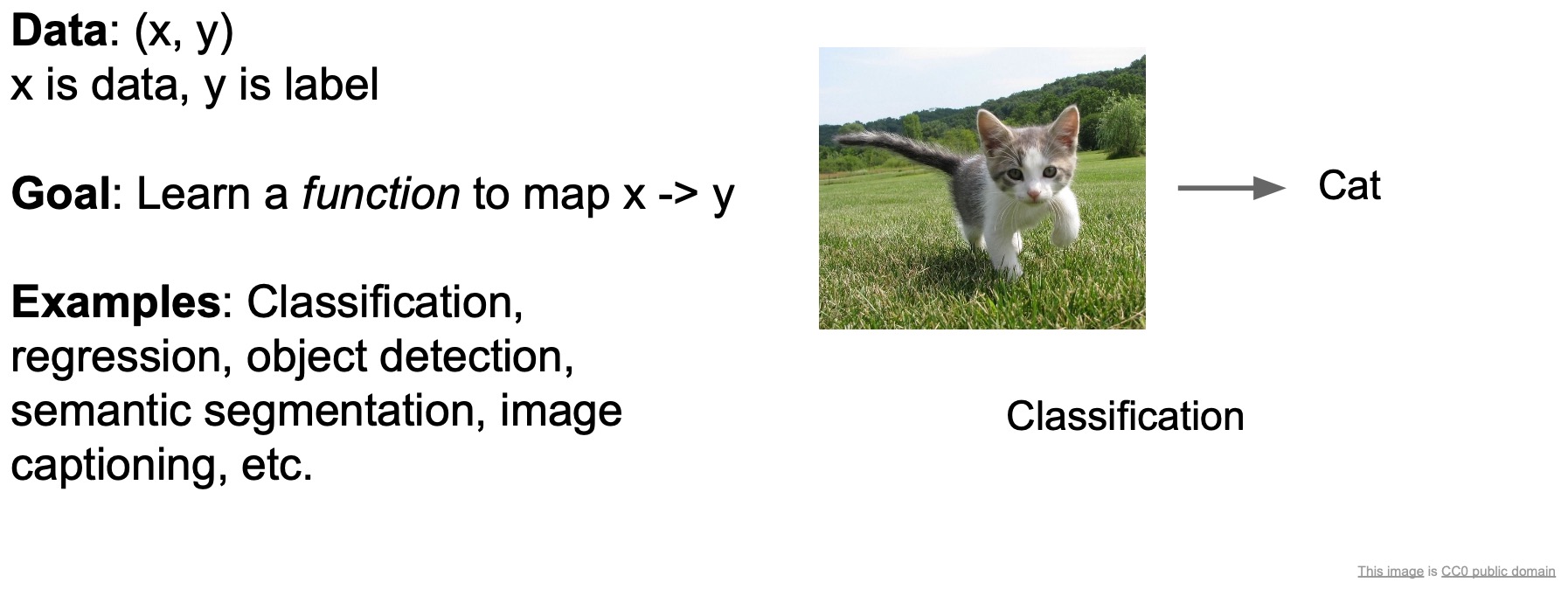
- So far we’be been talking about supervised learning. This is a problem where you have data \(X\) and labels \(Y\) and your goal is to learn a function that maps from the data \(X\) \(\rightarrow\) labels \(Y\). Some examples of this are classification, regression, object detection etc.
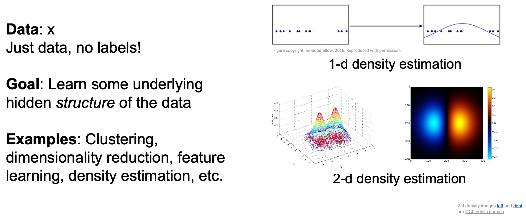
- We’ve also talked about unsupervised learning where you only have the data and no labels. The goal here is to learn some underlying hidden structure in the data. For e.g., clustering, dimensonality reduction, density estimation, generative models are pretty good examples of this type of learning.
- Today, we’re going to talk about a different type of problem – the reinforcement learning problem.
Reinforcement Learnings: The Basics
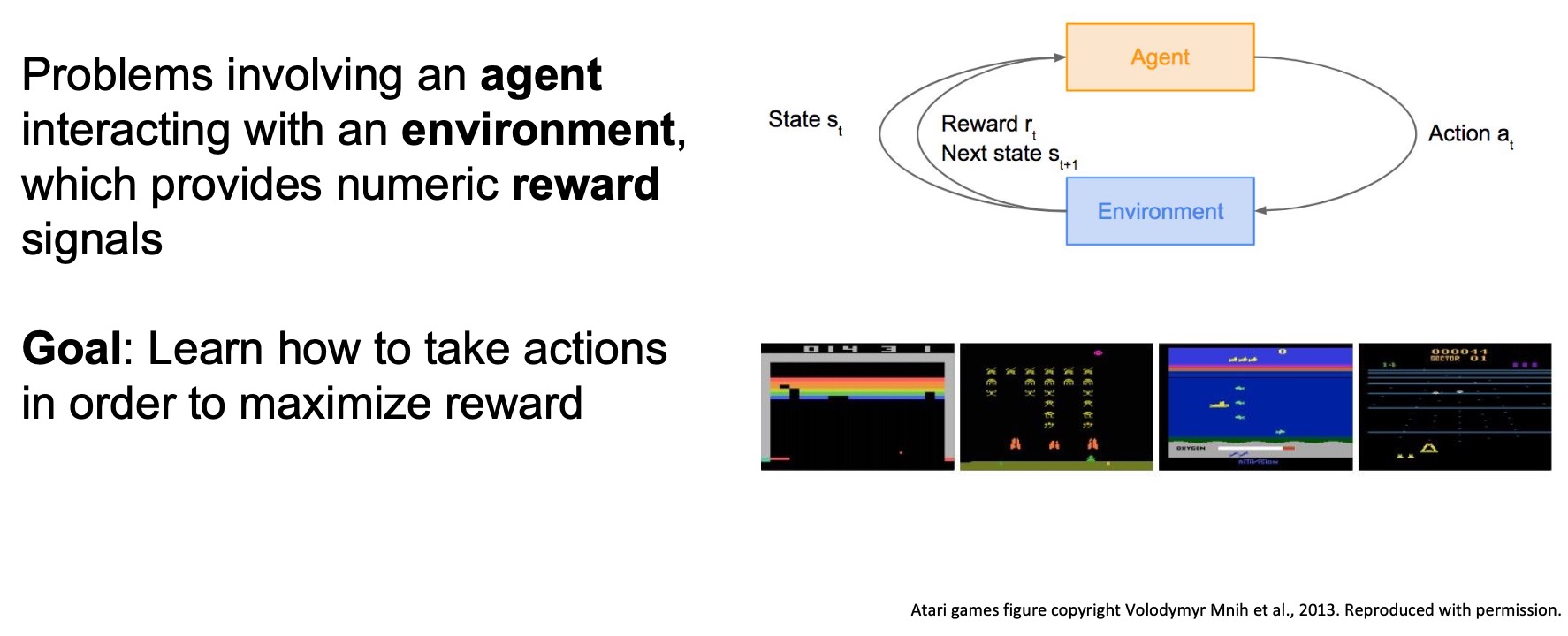
- In Reinforcement Learning (RL), we have an agent that can take actions in an environment and receive rewards for its actions. The goal is to learn how to take actions in a way that can maximizes the rewards that the agent sees.
- At a high level, this will be different from what you’ve seen before for a couple of reasons:
- There’s indirect supervision happening through this reward that the agent obtains
- The agent is actually responsible for collecting its own data so we’re not going to provide it data explicitly – it has to choose what data it encounters.
- The problem is sequential in nature.
What is Reinforcement Learning?
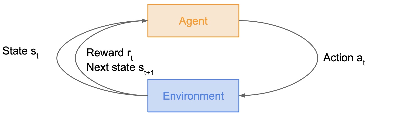
- In the RL setup, we have an agent and an environment and the agent is interacting with the environment.
- The figure below illustrates an episode of interaction between the agent and the environment:
- The environment gives the agent a state \(s_t\) for observation.
- The agent takes an action \(a_t\).
- The environment responds to this action by giving the agent a reward \(r_t\).
- The environment transitions to the next state \(s_{t+1}\).
- This process repeats until the environment reaches a terminal state/goal which ends the episode of interaction.
- RL problems are characterized by 6 parameters:
- Objective
- Agent
- Environment
- State
- Action
- Reward
Cart-Pole Problem
- Here’s a Cart-Pole problem where the objective is to for the agent to balance a pole on top of a moveable cart.
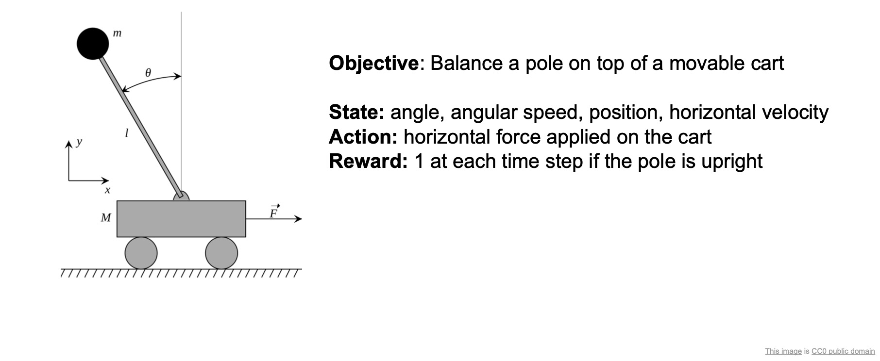
- The state can include things like the angle between the pole and the vertical, the angular speed of the pole, the position and horizontal velocity of the cart – these are all decision variables that you might need to have in order to make good decisions on what to do next.
- The action space includes the action of appplying a certain amount of horizontal force on the cart. This is what the agent has to decide at every time step – how much force should I apply to the cart?
- The reward is 1 for each time step if the pole is upright. So, maximizing this reward is going to ensure that the agent learns to keep the pole upright.
Robot Locomotion
- Another example is robot locomotion, as shown below.
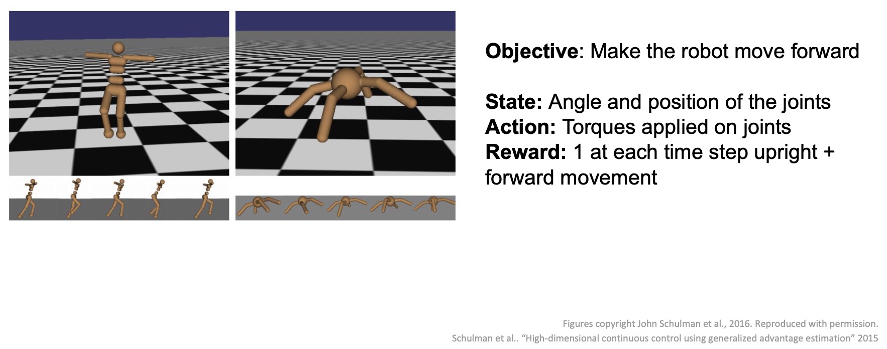
- There’s a humanoid robot and an ant-robot model shown here in the above diagram.
- The objective is to make the robot move forward.
- The states might be the angles and positions of each of the joints.
- The action would be the torque to apply to each joint in order to move the robot.
- The reward might be 1 for every time step the robot is upright and for every time step where he actually gets some forward movement.
Games
- Games are also a big class of problems that can be formulated with RL.
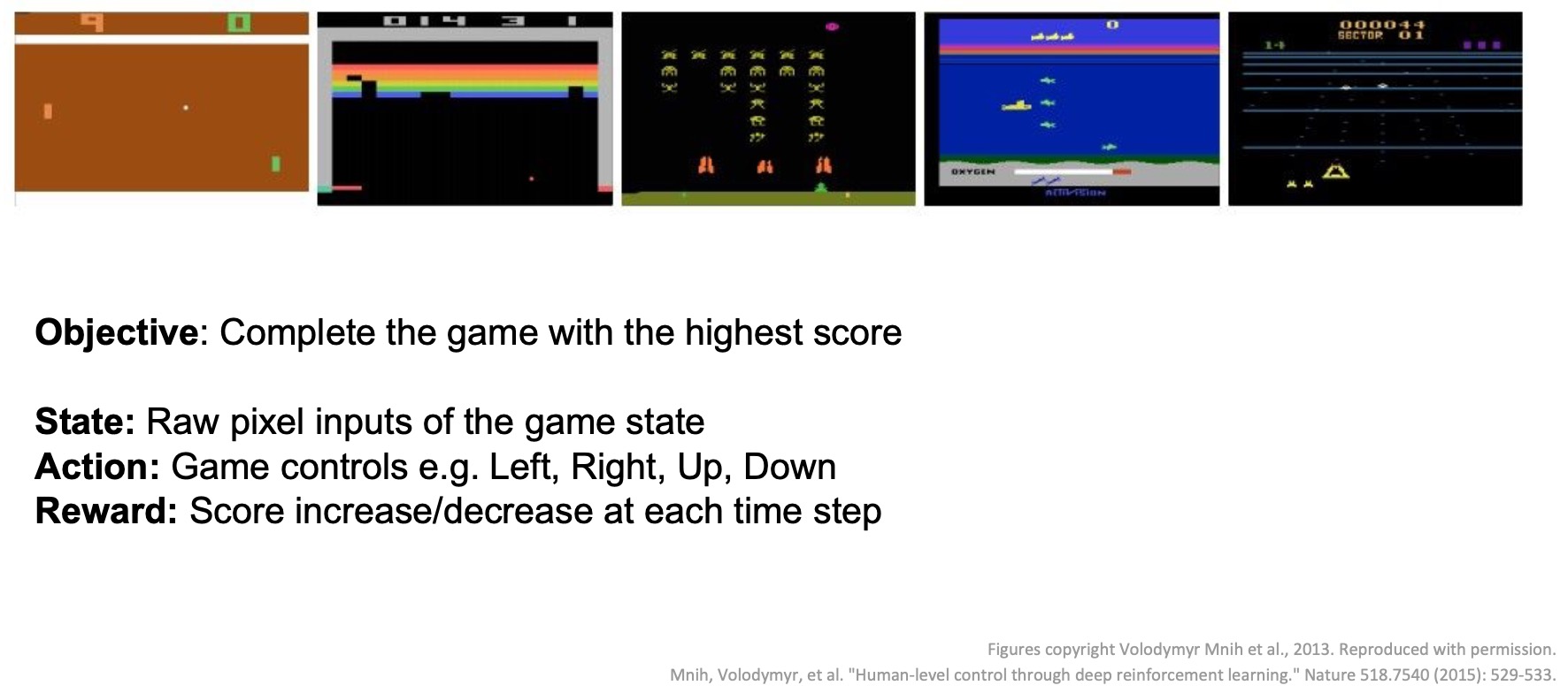
- For e.g., we have Atari games which are a well-known success of deep RL.
- The agent is a player trying to play these games using visual inputs and game controls.
- The objective is to maximize the score or play the game as well as you can.
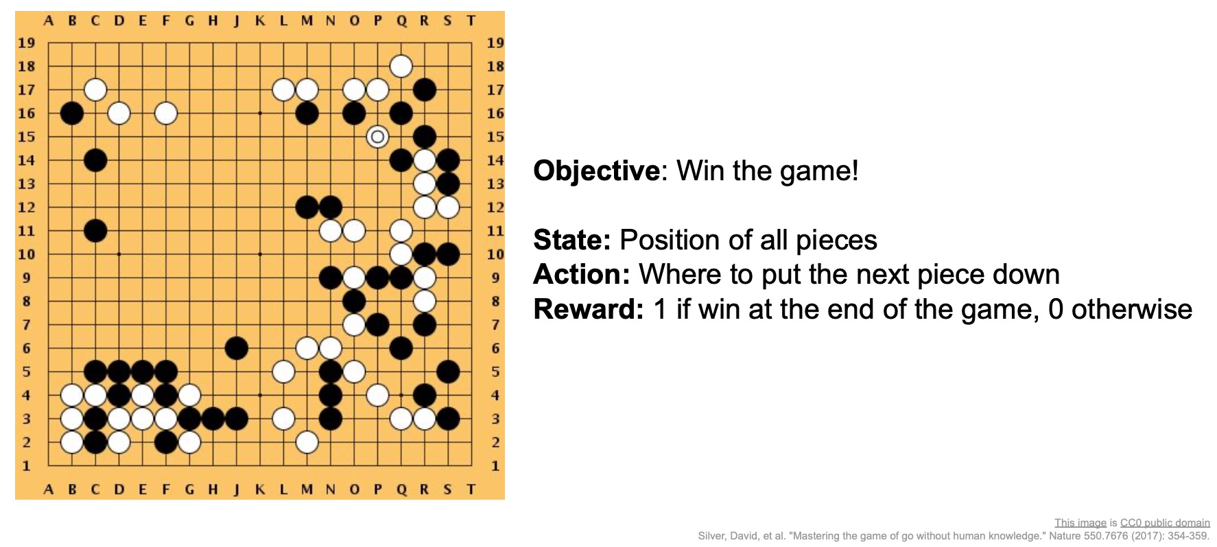
- In 2016, a huge milestone in this field was reached when DeepMind’s AlphaGo beat Lee Sedol, the best Go player in the history of the game.
- Playing the game of Go was formulated as a reinforcement learning problem.
- The state here was basically the position of all the pieces.
- The action was where to put the next piece down.
- The reward was 1 if you win the game or 0 otherwise.
Markov Decision Processes (MDPs)
- MDPs help formalize the RL problem, which is the sequential interaction between the agent and the environment.
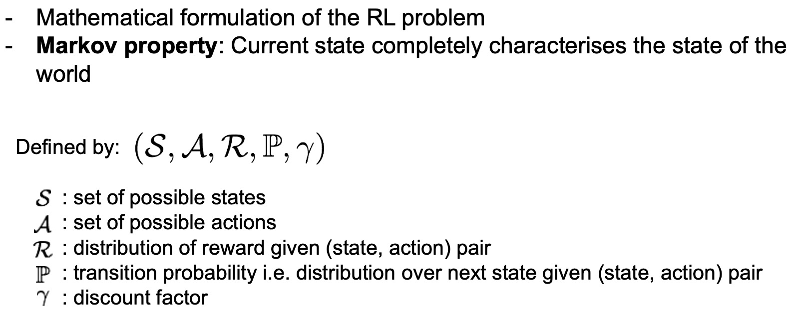
- Shown below is a mathematical formulation of the RL problem. MDPs satisfy the Markov property, a key property which says that the current environment state completely summarizes everything I need to know about the world and how it can change. In essence, that means that by only looking at the current state of the world, I’m able to make my decision in such a way that I can perform well at the task at hand.
- MDPs are defined by a tuple of objects: \((S,\,A,\,R,\,P,\,\gamma)\)
- where,
- \(S\) is the state space.
- \(A\) is the action space.
- \(R\) is the reward function or distribution, which is conditioned on state action pairs.
- \(P\) is the transition probability, which tells us how does the world transition from one state to the next conditioned on the current state and an action that the agent takes.
- \(\gamma\) is the discount factor, which tells us how much we value rewards now vs. later.
- where,
- Here’s how an episode of interaction works between the agent and environment:
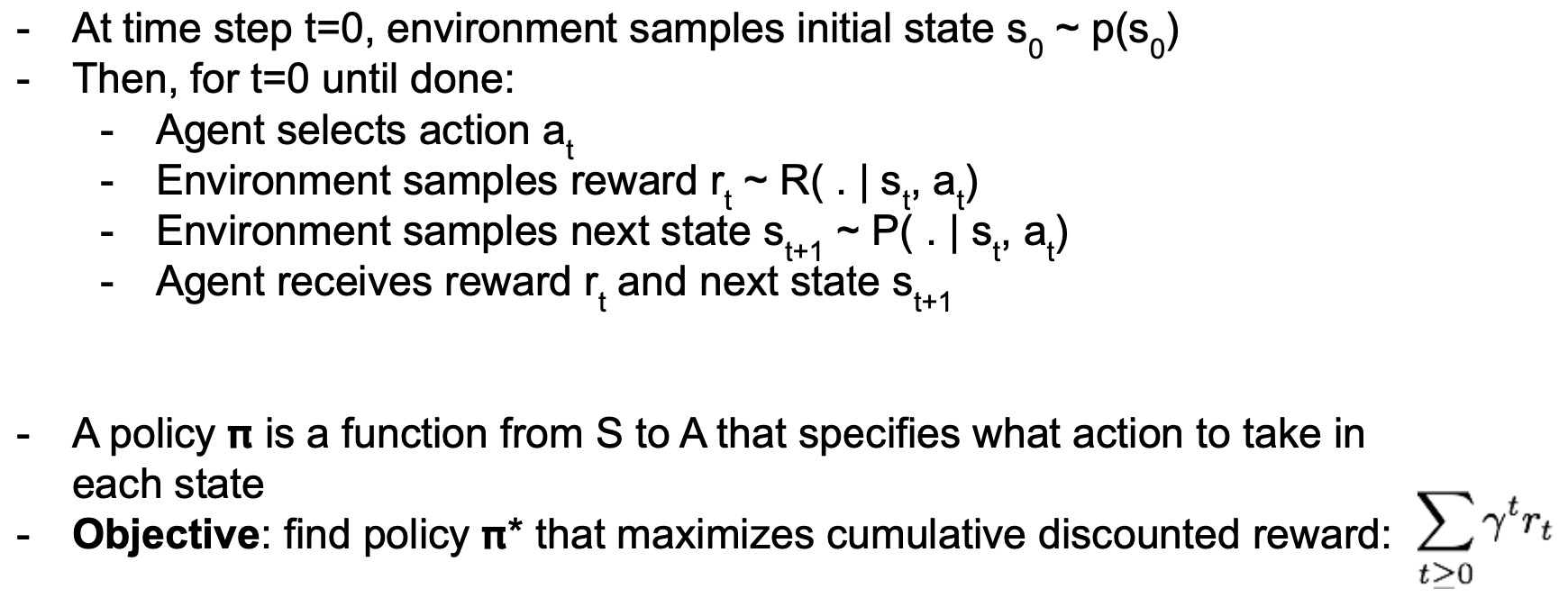
- At time step \(t\,=\,0\), we begin a new episode of interaction where the environment samples an initial state \(s_0\,\sim\,p(s_0)\) and places the agent in that state in the world.
- Next, we repeat the following:
- The agent selects an action \(a_t\).
- The environment then takes that action and responds with both our reward \(r_t\) and the next state \(s_{t+1}\) according to their world and transition distributions.
- The agent receives the reward \(r_t\) and the next state \(s_{t+1}\), and then selects the next action \(a_{t+1}\).
- This loop continues until the end of the episode.
- Next, let’s talk about an agent’s decision-making process.
- Policy:
- A policy is a function the maps \(states\,\rightarrow\,actions\) or more generally a distribution of actions conditioned on states.
- It’s basically a set of rules that tell the agent what to do in every conceivable situation.
- Note that some decision-making rules are going to be better in terms of maximizing your rewards than others.
- Objective:
- To find the best policy \(\pi^*\) or in other words, the best decision-making rule, that maximizes the cumulative discounted reward \(\sum\limits_{t\geq0} \gamma^t r_t\).
- The discount factor \(\gamma\) basically tells us how much do we care about rewards later vs. now.
- Policy:
Horizon of the Problem
- Does the horizon of the problem matter? Yes, it does!
- The horizon of the problem is defined by the number of steps the agent gets to interacts with the environment.
- When we talk about an MDP, a reward is offered at every single time step to the agent, but the agent has a certain horizon to play in the environment (characterized by the dicount \(\gamma\)) with the ultimate overarching goal of trying to maximize the sum of rewards.
- So the horizon definitely does matter. This has been one of the ongoing research questions in reinforcement learning which is how hard are longer horizon problems vs. shorter horizon problems.
- In the limiting case, if we just have to make a decision once and then we’re done with the episode, which seems intuitively a little bit easier, than having to make a long structured sequence of actions in order to achieve a task.
- In the theory of RL, the horizon of the problem does play an important role in both the definition and the difficulty of the problem.
The Problem of Spare Rewards
- In some cases, a reward can be sparse in a problem because we only know how to check success vs. failure but we don’t really know how to write down our reward function that will enable good behavior, i.e., which gives more dense supervision along the way.
- This is actually a classic problem especially in Robotics because sometimes we might know how to tell whether a task was successful or not, for e.g., if a robot has successfully lifted an object but knowing what type of reward function would guide the agent through this behavior isn’t straightforward. This can be hard because the agent needs to explore the action space and if it’s getting no rewards for the longest period of time until it accidentally lifts the object, it’s going to be a very hard problem to solve.
- Some fixes for this:
- Imitation learning: Learn the reward function from demonstrations of the task.
Simple MDP: Grid World
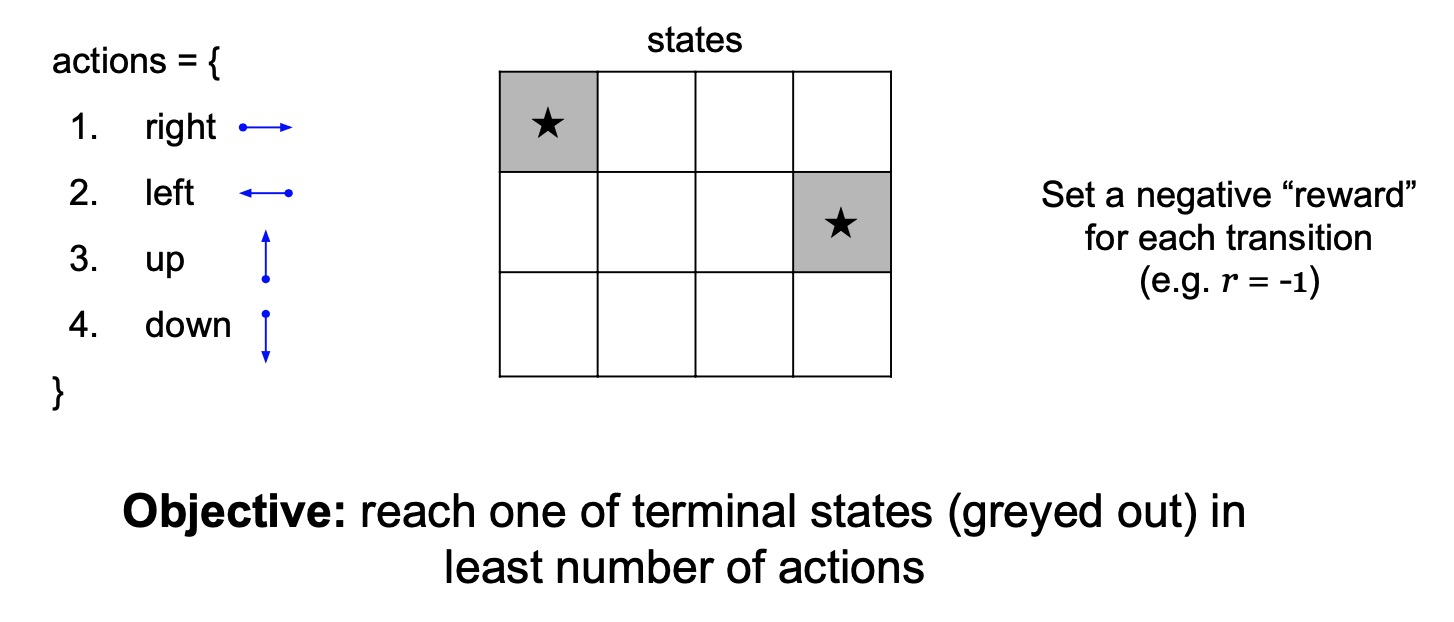
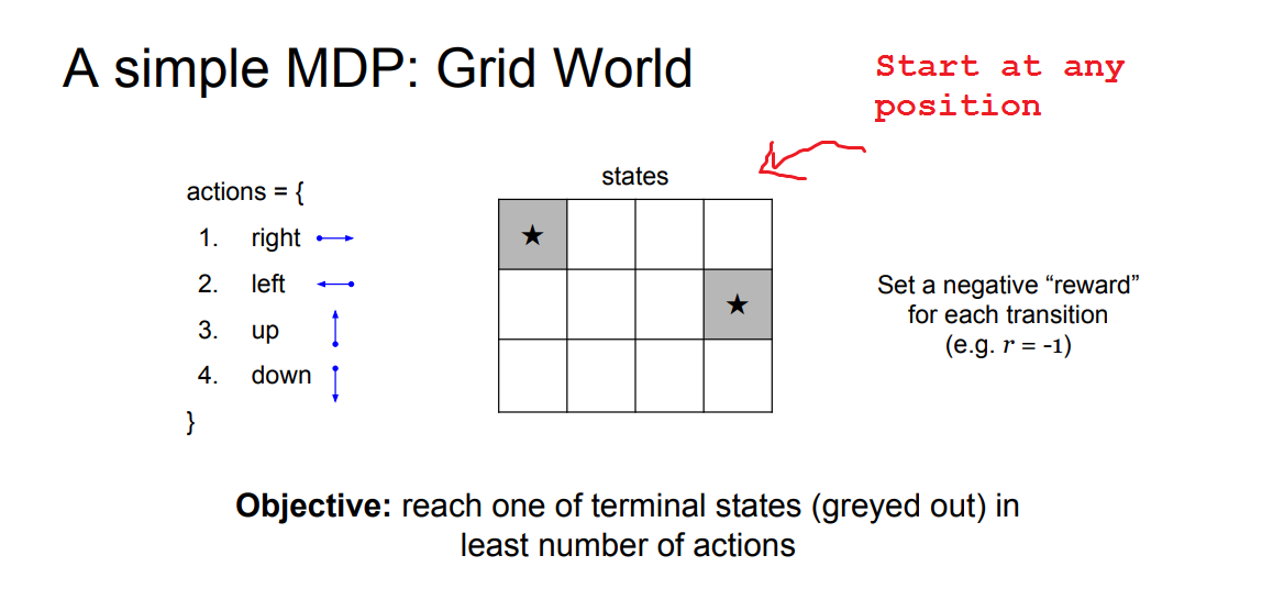
- Shown below is a simple grid world example of an MDP.
- RL problem characteristics:
- The states are a discrete set of cells.
- The actions are to move right left up or down in this grid world.
- The reward function is that we get a negative reward for each transition (which implies, that we should be using the least number of steps to get to our terminal state).
- The goal (terminal state) is to reach one of these gray states as fast as possible.
Simple MDP: Types of Policies
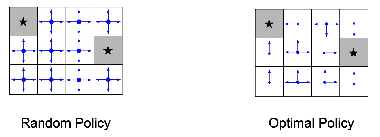
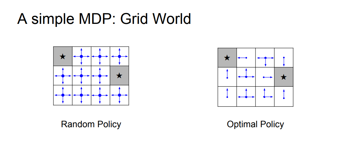
- We’re going to compare two different policies or decision-making rules here.
- Random policy: simply sample a random direction in every single grid cell at any given time step \(t\).
- Optimal policy: tells us what are the possible actions that can be taken in every single grid cell such that we’ll need minimum number of time steps to reach the goal.
Simple MDP: Finding the Optimal Policy
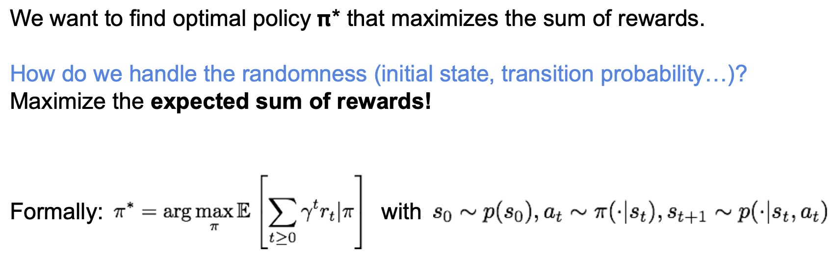
- We’re looking to find the optimal policy \(\pi^*\) that maximizes the sum of (discounted) rewards.
- This is going to be a decision-making rule that essentially tells us what to do in each grid cell.
- There can be a lot of randomness in the world with environmental aspects such as the initial state, the transitions, etc.
- Thus, the question arises: how can we characterize the performance of our policies given all these sources of randomness?
- Answer: We’ll maximize the expected some of the rewards.
- Formally, this is the RL problem (shown below). Our job is to find the best policy that maximizes the expected sum of rewards where we have randomness in the following:
- Start state
- Actions we choose if our policy as a distribution instead of a deterministic mapping
- How the world responds to our actions through the transition distribution.
- Before we talk about how to find the optimal policy, lets look into metrics that enable us to pick the best policy, namely the value function and Q function.
Value Function
-
The value function of a state \(s\) is the average sum of rewards, i.e., the average return, that you can get if you start at that state and follow the policy (or the decision making rule) \(\pi\).
- For a given policy (or decision-making rule), we sample many episodes of interaction starting from that start state. Next, we sum up all the rewards and average it out.
- Why is this useful?
- A value function offers an objective metric to compare one policy vs. another. Compare the value functions of two policies at a given state \(s\) can help us find the better policy, since it will have a higher value function at that state \(s\).
Q Function / Q-Value Function / State Action Value Function
- A Q value function (or state action value function) is very similar to the value function except that we can take a different action at the first time step.
- Why is this useful?
- Sometimes we want to consider what would happen if we deviate from our decision making rule for the first time step \(t\,=\,0\), by evaluating the impact of choosing a different action \(a\).
- Intuitively, if deviating from \(\pi\) by choosing a different action \(a\) achieves higher value, then \(\pi\) can’t be optimal since there’s actually a better strategy that exists.
Q-Learning
- Q-Learning and Policy Gradients are the two major classes of RL algorithms.
- The optimal Q-value function \(Q^*\) is given by the highest expected some rewards we can achieve in a given state \(s\), after following a given action \(a\).
- In other words, we’re looking to find the best policy/decision-making rule after a given action \(a\) that maximizes sum of the rewards with \(Q^*\) as the average return.
- Bellman equation
- One of the most fundamental ideas in RL the bellman equation.
- Given an optimal Q-value function \(Q*\) which is the best you can do in a given \((state, action)\) pair, at the next time step you would better continue doing the same thing.
- In other words, assume you take action \(a\) in state \(s\). When you end up in the next state \(s’\), the best thing for you to do is to select the action that maximizes my value which implies that we should maximize the Q function over actions in the next state.
- As always, we use an expectation because we’re going to have randomness over what state we’re going to end up in after taking that action \(a\) in the original state.
- If \(Q^*\) is the best you can do for any action, then the best policy is just going to take a maximum over actions at the current state. So the optimal policy \(\pi^*\) is just the best action that maximizes \(Q^*\).
- One of the big advantages of using value functions is that they remove the temporal aspect of the problem by summarizing everything that’s going to happen later so you can reduce it to a one step decision-making, which is simply to look at all your actions and pick the best one according to your Q function.
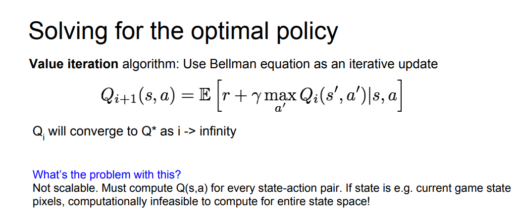
Solve for the optimal policy
- Given the bellman equation, how do we solve for the optimal policy?
- one x one algorithm is called value iteration and it uses the bellman equation as an iterative update so here’s what we do
- i initialize my current Q values for every state in action at random and then I’ll plug these Q values into the right-hand side of the bellman equation and use it to extract a new set of Q values that’s the left-hand side so this is just an iterative update and notice that when I reach a fixed point which means my current Q values don’t change after an iteration that means the left-hand side equals the right-hand side the Q funk u function all my Q values will satisfy this equation um that means that the fixed point of this update rule is the as a bellman equation and thus it must be optimal so now the natural question is can I be sure to always reach a fixed point by iteratively applying this update there’s a remarkable fact the bellman update is what’s known as a contraction mapping what this means is if I do this update again and again and again I’m guaranteed to converge feet to the fixed point which is also the optimal Q function Q star so that’s exactly what value iteration does what seems reasonable but what’s the problem with this it’s not scalable we saw the grid world earlier what if we had a huge grid lots of states and lots of actions possible per state or we had a continuous space instead of a discrete one like image observations in Atari we can’t store a table of Q values for every single state and every single action so what’s the potential solution to this well why not just throw a function approximator edit let’s learn a mapping between state action pairs and give values instead of storing every single pair of inputs and outputs in a table.
- Neural Networks can serve as effective function approximators, so let’s try that so we’re going to use a function approximator and this is what’s going to lead us to something called deep Q learning, a common part of modern era artificial intelligence.
- If the function approximator is the function approximator is parameterize by a set of weights theta so these conduces you can think of this as the weights of our neural network and by varying these weights of my neural network we’re going to obtain different cue functions and the cue learning problem is now going to be find me the best set of neural network weights the best theta that’s going to get closest to the optimal Q function in this Q start and consequently produce the best behavior for my agent so how can we learn that
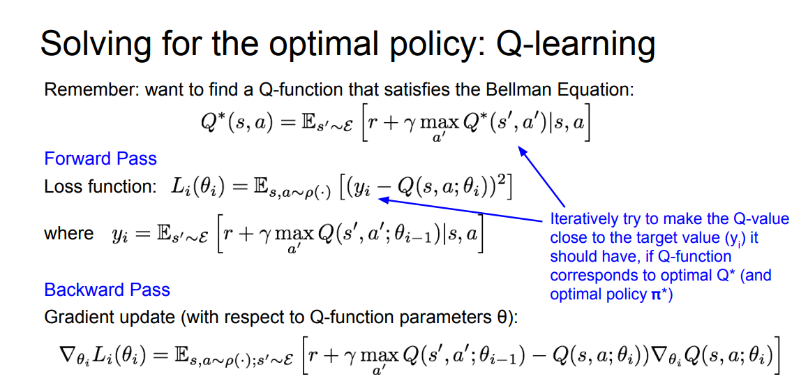
-
In RL almost everything is about the bellman equation so let’s start from there what we’re gonna do is we want to find a cute Q function that satisfies the bellman equation but and we would like to do something like value iteration but we don’t have a way to do an exact update we don’t know how to do this exact update in closed form but we do know how to do that propagation for neural networks so why don’t we just put a penalty on how much the current Q function D leads from the bellman equation I can look at the left-hand side and right-hand side of the bellman equation and I can say um how much does the current Q function how much error doesn’t achieve between the left hand right-hand side and I put an l2 loss on that so you can see here is y I is given by the right-hand side of the bellman equation it says with my current Q function what does the right-hand side look like and then the left-hand side is just my incurrent q function at the given state in action I put up a square L to us and I minimize that so that’s exactly what we’re gonna do and this is what is known as DQ learning I’m going to use a function approximator for my Q network and I’m going to approximately try and solve the bellman equation through a value iteration by keep by minimizing this l2 loss
-
okay I think it’s a good time to pause for questions well do you have any questions you like - yeah so there is a question that I think maybe need the longer answers we can leave that towards the end and there’s another question and maybe if it’s well err it’s what is the difference between an T P and Q learning bellman equation I assume the student means like the value function versus Q function and why is Q learning better I see so this is a good question and it can be sort of confusing at first why we want both the Q function and a value function the really nice thing about the Q function is that it lets you condition on state and action so this will let me evaluate how good my return is going to be for different choices of initial actions so this leads to a very nice way to extract a policy from a q function right if you go ahead and you hand me the best q function q sir my policy is just given by taking the max over all the actions to pick the best one um the value function I wouldn’t be able to immediately do that I need to do one more bellman back up to tell me which action to pick so that’s sort of a short answer along it’s longer answer would basically say that well let’s just leave it at that I think yeah that’s good yeah so the other question is basically on if we cannot find the equilibrium for the Markov chain what should we do but maybe we can assert that towards the end because it seems more yeah well we’ll say that one for the end okay cool Thanks I guess another here’s a case study she’s playing Atari games the objective was to complete the game with the highest score and this is what people did this is what did mine did actually they show that deep Q learning can work and you can get superhuman performance on Atari games from no prior domain knowledge so what did they do what they did is a parameter is the Q network using this type of you know deep convolutional network the input is a stack of four frames together the last four frames of the game and this is so that the network gets some information about things like movement like in breakout they have to it’s useful to get some information on which direction the ball is moving so then what they do is they process this stack of frames through some convolution layers and then some fully connected layers and finally the last fully connected layer has four outputs one output per action here there are four actions in the scheme and that corresponds to the different Q values per action so this is are really nice because we’re actually from one forward pass getting the Q values for all our actions so it’s efficient and just to mention here other Atari games can have action spaces between 4 and 18 so depending on that the change the the size of the last layer changes oh yeah this is what I already mentioned one single feed-forward pass you get all your actions action values so this is nice but there’s a few more tricks we need to actually hit the store can practice one big problem with the current way we formulated the problem is this sort of nasty regression we’re doing we’re doing minimizing this l2 loss but if you look closely at the right-hand side on the left-hand side the target values and your you know initial Q values you’re trying to optimize your having this you’re actually labeling your data with the same network that you’re trying to optimize the target values are a function of Q right you would use your Q network at your last iteration to get these Y eyes these target network values sorry its target values and so what we have is I’m trying to both update data using this class but also generate labels on my data using the same theta so it’s like trying to hit a moving target in motion in one direction might go back into the update any map might get this nasty positive feedback loop so this is non-stationary problem is it addressed by using a target q network which is a slow-moving version of the Q Network we are learning think of it as a another network that lags several iterations behind the sort of current Q network and this target network will then be used to generate my target Q values when training the Q Network one other thing used here in order to get this to work in practice that I want to mention is something called experience replay learning from batches of consecutive samples is problematic because if we’re just playing the game and taking actions and taking these consecutive at samples and learning from it these samples are incredibly correlated to my current decision-making strategy and the current Q Network will determine the next training samples and this will lead to more positive and bad positive feedback loops so for example that and I’m trying to move left the training samples will be dominated by samples that all were coming from the moving left actually so how can we address this issue to get a better learning distribution the trick that most people use is called experience replay they keep a replay memory which is a huge sort of data set of past transitions in the game and you can think this is like the last end episodes that the agent has played and then we randomly sample mini batches from this large experience replay and this is nice because it also allows each transition to be used more than once we keep the data around for multiple learning updates so we’re more efficient with the samples that the agent collects so let’s put it all together well initialize the redo play memory and the cue network and the agents is gonna play em episodes in total this is going to be in full game episodes will initialize a start state then for each time step of the game what we’re gonna do is we’re gonna let the agent act in the world to collect data and what we’ll do is we’ll do what’s known as epsilon greedy we’re gonna try and do the best thing that our current q network would say is the best thing to do but we’re going to with probability epsilon choose a random action instead and this allows us to explore the environment and collect new data instead of completely biasing our data towards our how good our current q network is then we’ll take the action and observe the next reward and the next state and then this transition gets stored in the replay memory we’ll sample a random mini batch of transitions and learn using gradient descent and here is a video of Google’s or deep mines deep you learning algorithm in action so what happens here is maybe I should skip urine what’s really nice about this as I mentioned earlier is that there’s no domain knowledge involved basically it starts with just a hue Network in an empty replay buffered or experience replay and it learns to play this game directly from raw pixels without knowing any concepts like what ball is or what those rainbow stripes mean it’s just collecting its own experience plotting it into the buffer and training using the DQ learning algorithm and so that’s that was I believe after 10 minutes of training and then after just two hours the training no it starts playing very very well you and then if I skip ahead after four hours of training it discovers a pretty awesome strategy which is that digging a tunnel through the wall if any of you guys have played breakout this is a pretty class of strategy um by digging the tunnel through this brick barrier you end up very efficiently clearing out multiple blocks as you can see there so this seems really cool but what’s there’s still an issue with Killoren which is that the q function can be very complicated so depending on what type of domain or what type of tasks you’re trying to solve this can be hard to learn for example imagine you have a robot that’s trying to grasp an object there’s a very high dimensional State great raw images of your robot and your robot arm in the object it’s hard to learn the exact value of every single state action pair you see but on the other hand maybe the the policy parameterization can be much simpler you know you see where the object is located and then you move your hand towards the object or maybe if you’re near the object all you need to do is close your gripper so some motivates the question of can we learn a policy directly instead of trying to model this value function first and then extracting the policy this is what’s gonna bring us to policy greetings so first let’s define a class of parameterize policies uppercase PI here what this is is think of this as I have a whole family of models given by a single neural network this neural network takes an estate and outputs either an action or a distribution of actions that’s what my policy is and I’m gonna represent it with my neural network for each policy now I’m gonna define its value for a given beta a given set of parameters you give me this equation is telling me on the this is the expected sum of rewards that is the same thing that we’ve been using as what we want to maximize so the problem should be really to maximize the sum of rewards to find the best theta which is spuntz of the best policy now how do we do this we’re going to use gradient ascent on this objective to move the policy parameters to optimize this sum of Q mu the sum of rewards so let’s talk about how we’re going to do this the algorithm that comes out is called the reinforced algorithm so mathematically we’re gonna write out sample trajectory work we’re gonna write out future reward of trajectories as an expectation over the trajectories from the current policy so let’s think we sample trajectories of experience gameplay that we talked about with our current policy pipe data for each trajectory I can use some of three words and computer returned and then if I average all those returns that’s what my objective is I want to know we’re starting with an objective function here that only depends on the parameters of interest through the sampling distribution what does this say this says I have a current policy according to data and then generate a bunch of trajectories by sampling those trajectories according to PI and then average the returns so the only way this objective depends on theta is because I sampled those trajectories from theta and we all know that sampling is non differentiable in general so this is already starting to sound like a hard problem I want to optimize this function that only depends on my parameters by sampling or through sampling trajectories okay so let’s just try and differentiate and see what happens what happens is that we end up with this sort of intractable Sun because if you see I tried to differentiate through the expectation and this expectation is over all possible trajectories that I could ever see this gradient theta of P of theta conditioned on sorry P of tau conditioned theta is saying for all possible trajectories measure how lightly it isn’t that that trajectory could have been generated by my current policy given a probability distribution sort of likelihood or score and then differentiate through that but something over all possible trajectories is just not feasible you however we’re going to use one of the most powerful tricks in all of Matt which is multiplying by 1 we’re going to multiply the top and bottom by P of town which is the probability of a directory and then what you’ll notice is that we can rewrite this as a gradient of the watt because you know that by the chain rule the gradient of the log of a function is equal to the gradient of the function over the function that’s what’s going on there now we can rewrite this gradient as another expectation but now this gradient can be computed with Monte Carlo sampling so this is really the core idea of reinforced the probability of that what I’ve written here is the probability of a trajectory of states and actions conditioned on the policy for conditioning on theta what we’re gonna do here is we’re gonna take a lot of books cents and then we’re gonna differentiate this because this is what we wanted in the previous if you look at the bottom of the slide we want to compute the gradient of log of P of tau so after differentiating what we see is that the this gradient doesn’t actually depend on the transition probabilities which is really good news because we don’t actually assume we know that right we we assume that the agent has to collect its own experience but it doesn’t know how the world works and we shouldn’t require our algorithm to know how the world works so therefore we now have a way to estimate what we’re gonna call here the policy gradient which is the gradient of the cumulative reward with respect to the policy parameters and we have a way to do this purely through just sampling trajectories from the policy and estimating returns so I want to take a moment to just talk about why this is really really powerful we started with an objective function that only depended on the policy parameters through the sampling of these trajectories which was non differentiable but now using this reinforced trick we have a way to optimize a subjective and also treat the Returns which are the things we really care about as a blackbox function if you notice I don’t need to differentiate through this through these rewards I don’t need to understand how the environment gives me my returns I can treat them as a black box that’s just numbers that my environment is gonna give me after I roll out my policy a few times or collect trajectories from my policy a few times and we don’t need to know anything about the MDV dynamics either so now let’s give some intuition for why this is the correct grading estimator you might remember for neither earlier in the quarter or from you may be 229 or another machine learning course if I give you a label dataset you usually try to maximize a lot likelihood at the outputs let’s say Y given the inputs X that’s what log of P of Y given X would be here what we see is we see the actions generated by a current policy given the states so the Y’s are like the actions and the X’s are like the states and this gradient estimator is basically saying you should still do maximum likely should still maximize the likelihood of actions conditioned on the states we you should read weight how important each sample is according to how much return they generated if you get hired rewards you should push up how important it is to maximize the likelihood of those actions and if the return is low don’t try so hard to maximize the likelihood of those actions so it might seem kind of simplistic to say that if the trajectory is good then all its actions are good but in expectation it averages out you can actually show that this is an unbiased estimator so one of the problems with this approach though is that it suffers from high variance because a credit assignment is really hard how do we know that one actually was really really important to give us this really nice high return it’s unclear because we’re training multiple sampling operations together so how many trajectory is what I need to collect to get stable estimates of this policy grading it’s probably probably a lot because of these change sampling operations if I go ahead and I collect - let’s say collect two samples right from the same initial state using my policy those two trajectories are probably going to look very different from one another and that’s what contributes to the Siberians for this grading estimator so we’re going to now talk about what happens what can we do to reduce the variance of this estimator but I think this is a good time to pause for questions and well are there any questions and people would like to you know there’s one new question but I saw mark Monte Carlo and so the question goes like this and with Monte Carlo we see that in order to get precise results we often have to calculate many many samples due to its slow rate of convergence so basically that’s the fact that we are using Monte Carlo means we don’t care about how precise our calculation of the gradient is I see I think another way to rephrase this question is exactly the high variance sort of issue in order to get a very stable grading estimate because of this high variance problem we’d have to collect a lot of samples from the policy at every iteration what we have to do to get a very good estimate of this policy grading is a collect a lot of trajectories because what happens for a high variance estimator is if I collect and trajectories once and then collect and trajectories again those two when I compute gradient estimators for those two different set of trajectories they’ll look very very different unless I know is sufficiently large so to get stable training I would need to collect a large number of trajectories because of the fact that we’re using Monte Carlo and because of the fact that the sampling procedure over time means that lots of different possibilities are possible and that’s why we want to reduce the variance of this estimator so we can get we don’t have to collect as many trajectories per iteration and we can have more stable learning where it’s not as stochastic well thank you god that slow any question about that’s here awesome so now let’s talk about very introduction it’s an important area of research and policy greetings let’s look at some first naive ways that we can do is first send you is that when you look at a given state action pair along the trajectory the whole return of that trajectory doesn’t matter because the whole processes of Markovian I should really only look at returns going on from that state I should pair and so what I can do is I can replace an inner return over the full trajectory with a truncated son which only looks forward from the current time step I’m considering why is this a good idea because having shorter sums over time will reduce the variance of these estimates because I’m doing less sampling chains over time here’s a second idea let’s use a discount factor to ignore delayed effects um so what this will do is it’ll say that what happens much later matters less and thus because you’re also down downplaying the imprints of later time steps this will lead to more stable estimates because you’re effectively summing over a shorter horizon there’s a third idea and his third idea is often called learning a baseline function to reduce the variance here’s the key idea only relative orderings matter when trend up wait or downwind action likelihoods basically we can first think about how much return we expect to see in a given state and then see what actions let us do better then then then what we see here and then what actions let us do worse than this baseline so concretely the estimator it looks like this now I take the sum of her words and then subtract the baseline value those that give us returns that are higher than the baseline value be up weighted those that are lower should be down so how can I choose this baseline a good baseline would tell us how much return to expect from a state does this sound familiar it should remind you of value functions basically we’re trying to learn or understand how much better is an action than the return we expect this is actually given by taking the state action value and then subtracting off the value so this is basically the q function minus the value function now if we plug this in as our scaling factor of how much we want to push up or down the probability of our actions we Candice estimate the term in the parentheses is often called the advantage function which is pretty clear it’s telling us the advantage of taking an action as opposed to going with what the policy would have done now the problem is that we don’t know Q and B can we learn them and the answer is yes by using humor we can combine Paul’s ingredients with Q learning by both training and actor the policy and a critic the key function as opposed to key learning this critic only needs to learn what’s good and bad local to data generated by the actor in order to compute these scale factors so it’s not as difficult as Q learning where you had to learn a value function that really tells us what’s best everywhere because the policy needs to be derived from that q function here we’re learning the actor or the policy separately and the critic or Q function is only telling us what’s good and what’s that and of course he can also include all these different key learning tricks like experience replay so here’s a full actor critic algorithm in this reinforced framework will sample M trajectories under the current policy and then for each time step of each trajectory will compute the advantage function and scaled a log likelihood policy actions with this advantage function and we’ll backdrop on this last update the policy then we’ll update the critic using these observed Monte Carlo returns so this is doing regression to fit the critic all right so here’s reinforced in action this is a recurrent attention model and this is a very cool example of rainforests these models are often referred to as Hart attention and they’ve recently been seen in a lot of computer vision tasks for various purposes so the idea is this this model is going to learn a classification how to classify different numbers based on the glimpses of the image because only different parts of the image might be relevant to classifying whether this number is a - it’s got some inspiration from human perception and eye movements when I look at an image I might attend to very discrete parts of the image to understand what I’m looking at and the key thing here is that these glimpses are non differentiable because I need to select how to carve out a crop of this image and how after choosing that crop I might want to choose another crop and another crop all of which are non differentiable actions so this sound starts to sound a lot like reinforce we should learn a policy for how to take these glimps actions using reinforced such that I maximize my class classification accuracy and that’s what we’re gonna do um we look at a series of glimpses this is almost like an NDP right at every single state which is the current image I’m going to look at choosing another glimpse and so this is what it looks like in practice I’m going to basically choose a series of coins and quinces using this RNN such that I maximize my classification score I think I can pause for questions here yeah so there is one more new question Arthur Williams is same as say 10 C Maps hmm so these glimpses are sort of different because these glimpses are basically telling us it’s it’s a heart it’s also called heart attention rate as long as we’re precisely do I want to look so to discrete decision um saline C maps are sort of or these sort of like heat maps are a little bit more soft in that they’ll cover the full image it’s sort of more related to soft attention where I’m going to place weights on different parts of the image um this is heart attention this is saying I’m actually going to make you force force me to choose a little crop of the image that you want to pay attention to that’s the only question for now cool okay so now we’re going to talk about some more recent deep RL methods that have been used quite a bit recently the first is called proximal policy optimization and I want to quickly note that there are two versions in this algorithm and I’m only describing one and for lack of time and for trying to make it more understandable so the if you remember this is our policy gradient with a baseline function right it’s basically weighted maximum likelihood where the weights are coming from the advantage function now we’ve got this new objective for approximate for PTO I mean this objective comes from something called conservative policy iteration so let’s take a look and decompose what’s going on here this objective function says well I’m still gonna keep my advantage weights but the way I measure instead of maximizing likelihood I’m going to maximize the ratio of the lighten that the probability mass of my current policy to my old policy my old policy is a policy from the previous iteration and basically what this says is if my advantage weights are high I should try to place more probability mass on this state action pair compared to my what my old policy would have done and if my advantage weights aren’t that good then I shouldn’t place as much importance over increasing the probability of mass at that state action there and now I also have a constraint this constraint says don’t move your policy too much iteration to iteration keep the KL divergence between your old policy and your new iterate small and so what we’re gonna do is we’re going to take this objective and we’re gonna relax it this is a commonly used trick in optimizations to turn a hard constraint into a soft constraint so we’ve got this relaxation where I basically took this pretty much the Lagrange multiplier beta and moved it into the objective and now PPO adds one more key optimization which is we can tune this penalty with beta on how much I care about minimizing the KL divergence between my old and new policy adaptively based on the kale violation if my kale violation becomes very very small I can reduce my penalty and if money Cayla by elation it becomes much becomes too large then I can increase my penalty that’s a typo at the bottom it should be a greater than sign we’ll fix it later but basically the intuition is that this is going to work better than just having a fixed penalty we should increase the penalty when we when the KL violation becomes too large and then we should decrease the penalty when the kale violation becomes too small there has been many recent efforts to scale up our Elle and here’s one from Oban e eye on the game of dota 2 where they applied ppl at scale they collected basically their agents would collect 180 years of self play per day and they used a lot of compute 256 GPUs and 128 thousand CPU cores and they ran this in this whole distributed reinforcement learning framework where they’re basically scale up the amount of data they could collect through policy rules that put it all on the collect all there’s all this data and then they learn from it using the PPO objective so basically a really nice sort of takeaway from this is that with relatively simple algorithms that we have today if you scale them up it might be possible to achieve some pretty impressive things another recent algorithm is called soft doctor critic hide they operate in this framework of entropy regularized RL which is becoming more and more relevant today or more and more let’s say there’s a lot of recent works that use this paradigm the idea is forward the policy for producing multimodal actions policies have receive an entropy bonus entropy reward bonus for making sure that they don’t converge to a single action too quickly so under entropy regularization we can learn a hue function and this is often called a soft cue function the reason is gonna become clear in a second usually when we have a cue function we know the best thing to do to get the best policy is to maximize that cue function with respect to the actions but because of this entropy bonus in this case the best policy is a soft match to distribution over all the Q values um this is basically saying I the best thing to do is no longer to just pick the best or maximize the Q function with respect to the action but pick actions with probability proportional to the exponential of Q why does this make sense it makes sense because I’m rewarded for producing some entropy in my distribution I’m rewarded for maintaining some level of multi-modality and randomness in my actions and I should know this also really helps for exploration because I’m rewarded for not converging to actions single actions too quickly so it’s really cool that this algorithm has been used to Train physical robot policies in a matter of hours how you can see that robot at the bottom left learns to walk um this other robot learns to manipulate and turn this belt and in the middle that was learned from very low dimensional paste logic Nations you can see in the bottom right and then on the very rate you can see that this hosoi robot arm learns to stack Lego blocks so I also want to very briefly mention an application of RL which is policy learning and robotics this is a hard domain for several reasons there is a high dimensional action span or state space because if you’re trying to learn from images when you’re doing visual motor control these images are very can be much higher resolution or a much compared to just low dimensional observations of like let’s say the robot joints the robot needs to perceive the whole workspace and understand and identify what objects are important in order to accomplish the test so that can be pretty difficult the continuum that actions face is also continuous often we usually eye well it’s not like a target where I can just choose to go left right up or down now the the policy might need to choose a hold vector of actions such as how do I actually every single joint of my robot arm in order to reach different places and do what I want the robot to do of this it can also be hard for exploration how can we make sure that the policy is going to collect good and useful data when doing ha rel if I just use of completely random actions of the beginning how do I ensure that the arms even going to start making progress towards a table we’re all the good but where it’s likely I’m gonna need to manipulate this can be difficult and finally sample efficiency if I want to put this algorithm directly on a real robot I can’t have it just operate for days I mean you guys saw in there in the open AI five PT of application they needed to collect a hundred eighty years of experience simulated experience every day but in the real world we only have so many robot arms and you’re bottlenecked at the rate at which you can do data collection so sample efficiency becomes extremely key and also you don’t want to break your own arms so safety can be in issue as well so I just want to mention a few recent or you know lines of work that try and address this problem for robotics in the context of our l1 notion what approaches into real so in this approach you train with RL in many randomized simulation rooms and then you hope to generalize to the real world in this case the policy has even robust to perturbations at the end so here you can see a what they called a plush giraffe perturbation where an open a I trained this robot arm to solve a Rubik’s Cube another approach is annotation learning could imagine collecting data on a physical robot arm by letting a human to operate the robot arm using either a lid like a virtual reality device a smartphone or other input devices and then from this data we can train a policy using supervised learning to mimic or imitate what the human supervisor did and this could even be combined with RL right you can learn an okay policy from here and then you can start doing RL on top of that and that can get you a very good starting point from which you can start doing RL and I should also mention that this can also help in the case where someone brought up sometimes you have sparse award functions on if you have sparse or work functions in the real world this will maybe make it more likely that you’ve achieved the task with some random exploration some of the time and start to get useful feedback in the RL process a third approach or line of work is called batch reinforcement learning and this is where policies are trained from large experience buffers so that are not necessarily expert data and this has been becoming more and more popular just as recently as this year in last year and the idea you can think of this as what if I take my DQ Network right and I look at the experience buffer and I take that experience buffer and just treat that as a dataset and my goal is to back out a policy without any additional data collection is to do as well as I can from looking at that experience buffer from past episodes of interaction and trying to filter out what is good data and what is that date there’s a whole line of work on playing the game of go also in competing with humans whole line of work has gone mostly through deep mind and they had some really awesome successes where they mainly trained their algorithms first was alphago where they move instruct from human play right so this is similar to using imitation learning first and then doing reinforcement learning on top of it and then they had alphago zero where they simplified their version of alphago where they don’t need human play anymore there’s a completely used self play data where in an agent plays against itself many many times to understand what’s good and what’s not good and they had more updates on top of that and Lisa Dahl retired just a few months ago it’s a slightly sad story about how advances in a I might have adverse effects so just to summarize um policy gradients are very general because you’re directly taking gradient doing gradient descent on the policy parameters and the the main drawback though is that they suffer from high variance so it requires for a lot of samples to learn efficiently um the challenge here is sample efficiency by contrast there’s QQ learning which doesn’t always work because it can be hard to model the value function instead of directly learning a policy but when it does work it’s usually a lot more simple efficient because you can have a whole experience replay and you can reuse your data and you have a more stable learning a trip objective that doesn’t vary as much but the challenge here can also be exploration ashen mission exploration is a challenge in both cases and RL in general and as far as theoretical guarantees on policy gradients are guaranteed to converge to a local minima of our objective which is you know the returns of the policy often this can be good enough and q-learning by contrast has zero guarantees because you’re learning with this incredibly biased update of this bellman update approximating the bellman equation with this complicated function approximator and in fact a lot of recent work has gone into explaining how how unstable this type of learning is and why combining function approximation with a bellman equation can lead to pretty strong divergence in terms of what you want to learn and yeah I guess we can pause for questions here see people are questions oh cool so I believe this is kinda the second to last slide of the day right hmm okay so maybe we’ll help out too by student life question as well wait if anyone wants to ask a question please raise your hand and up meet you as always and yeah so first quick question I guess though for the heart attention part is the grams initialized randomly or I guess is asking how do we choose the first glimps I guess I believe it’s initialized randomly in the sense that I don’t think they they train using any sort of annotation I believe it’s straight from scratch and then the second question is is that the one we put it off till the question goes like this after otis veto it’s the optimal policy in in this case related to the Calabrian distribution tie for a Markov chain if so what are called what occurs in the case if our Markov chain is recurrent orphans that transient and has has no equilibrium distribution okay trying to unpack so I believe that when we talk about equilibrium distribution of Markov chain um the thing is that this Markov decision processes are a little bit more general than just a simple Markov chain because you can think of it as when you supply me a policy then I get a Markov chain because when you give me a policy you’ve told me how you plan to act in every single state so now the transition dynamics for the Markov chain only depend on the current state like we’ve removed the actions completely from the process so in that sense is the optimal policy related to the equilibrium distribution for the Markov chain um not really I guess if you any policy induces an equilibrium distribution for the Markov chain in a sense and it depending on you know what it chooses to do right it might be for example let’s say that you’re trying to in the grid world example right um the optimal policy always chooses to go to one of the two goal states depending on where it’s initialized right so once you given me that optimal policy you’ve induced a equilibrium distribution where no matter where I start I’m going to end up in those states in that sense it is related to equilibrium distribution because that policy the way it acts is no matter where you start I’m going to converge to those states Thanks that’s the last question does anyone want to ask a question life okay I think yeah I don’t see anyone raising their hand so okay it’s actually hi so I just had a quick question in terms of is this policy kind of related to determining like the transition probability of the mark of Inman yeah you mean policy learning in general or demean so yeah like when we when we choose like our policy and then is that decide just kind of give us the transition probability for that time step on terms of power of like how we act so I kind of like how it relates to because like in regards to what you just said in terms of how it relates to like we have like we choose a policy and then that kind of relates to like getting us like an equilibrium distribution so like if we choose a policy does that relate to like the transition probability and like this Markov chain kind of is that like am i interpreting that correctly or is that yeah let me let me go to the slide where we define the what a Markov decision process so you can you can see here right um that at when we sample the next state right that’s given by this transition distribution right P of s prime given s and a right so my comment was basically generally when you talk about standard Markov chains you only have this transition like matrix or distribution right here best friend given s just how does the next state fall from the current state in this case we have a transition distribution that’s conditioned on what actions you choose to take but if someone already hands you a policy pi events right now I can just treat this as a new just Markov chain right because once you’ve given me the rule of how to act everywhere I’ve essentially got a new transition distribution right s prime equals R is given by P of s prime conditioned on s and PI or s effectively because PI will always determine the action set make sense basically you can turn an MVP into just a Markov chain if you give me a policy or a rule that tells me what i’m going to do in every single state god i’m existence thank you you I just needed a nose um sorry could you please repeat the intuition with me huh find the balance equation again thank you sure okay so the bellman equation intuition is this it’s it’s this in his temporal consistency saying someone tells you that they’ve given you the optimal Q function okay Q star so that is the best thing we can do in a state after taking an action right um so if someone tells you that’s the best we can do this is the bellman equation literally is a recursion recursion relation and in fact this is also this general bellman equation goes into something larger called dynamic programming it’s got obvious relationships - like dynamic programming in computer science so because of this recursion but it’s basically telling us that if you tell me that this is the best I can do at this state in action then it better be consistent with what happens at the next state right if this is the best then at the next state the value at the next state is gonna be given by maximizing my Q function at the next state over all actions if I didn’t have that Maxim maximization then this could not be the best right so just multi-step consistency saying that if I look at the next time step on my net my next time step decision-making is consistent with money current time step you it put and put otherwise it’s saying that my value the value of this fate and action is equal to the reward I get from this state in action plus the value I get from all subsequent time steps and the value of all subsequent time steps is given by V of s prime or max over a prime Q of s prime apron make sense thank you you if you have any please feel free to raise your hand someone to submit a question by a QA the question goes like this in robotics what are some good scenarios of using discrete action space versus using continuous action space especially things softer critics seems to work pretty good ok so it’s a good question um in most cases with closed-loop visual motor control that I’ve seen people choose to use continuous action spaces but you can imagine discrete action spaces in different scenarios right like maybe if I’m doing robot navigation maybe I can have a discrete action space of moving left right up or down right or there’s always ways to turn continuous action spaces into discrete action spaces um sometimes I can treat the problem of robotic grasping as of this production space too because if I’m always doing top-down grasping I only need to choose a grasp angle like I can discretize the grasp angle into bins and say make it a discrete action for which bin you want to pick which corresponds to how much you want to rotate your gripper before you move down and try and grasp enough object um with regards to soft dr. credit seeming to work pretty good um I should mention that these are all scenarios that these tasks are relatively short horizon and exploration can lead to some pretty decent results right off the bat right so if you look at the Sawyer I’m on the very right it already starts with the Lego brick in hand right you didn’t need to worry about picking up that first Lego brick um and it only works or as far as I know it only works in this configuration so if you start changing the configurations like where the Lego block brick is placed it would need to learn the new mapping so basically the the complexity of what you’re trying to learn can have a big impact on how what what algorithm will work well and what learning method can can give you good results on the problem um we briefly talked about how time horizon can also play play defect rate these tests are relatively short horizon right you don’t need many time steps to act for many time steps to put the Lego brick on top of the other Lego brick but if you think about other more complex scenarios um for example um how might we learn this sort of longer horizon task where the robot arm actually uncover scible rods of bread grabs the bulb and then puts it in the oven and then closes the oven door this sequential interaction can be a lot more challenging to learn via something like pure reinforcement learning and it can be a hard exploration problem and there are other methods that people have looked at for learning such situations and people have also been looking at not using RL from in its entirety what we what people call ended end but using it for different pieces and using other solutions and combining it with other solutions to work so that maybe RL shouldn’t be the only thing that we use as a problem-solving method but something that can fit into another method or group of methods I think that’s a great okay now is there any more question it’s like learn to be pretty good on time it’s not for this lecture cool I believe that should be it thanks for the lecture it’s really right I also learned a lot sorry and for next week we will have seen grass visual dino from Ranchi I believe cool
- Reinforcement learning problems are involving an agent interacting with an environment, which provides numeric reward signals.
- Steps are:
- Environment –> State
s[t]–> Agent –> Actiona[t]–> Environment –>Reward r[t]+ Next states[t+1]–> Agent –> and so on..
- Environment –> State
- Our goal is learn how to take actions in order to maximize reward.
- An example is Robot Locomotion:
- Objective: Make the robot move forward
- State: Angle and position of the joints
- Action: Torques applied on joints
- 1 at each time step upright + forward movement
- Another example is Atari Games:
- Deep learning has a good state of art in this problem.
- Objective: Complete the game with the highest score.
- State: Raw pixel inputs of the game state.
- Action: Game controls e.g. Left, Right, Up, Down
- Reward: Score increase/decrease at each time step
- Go game is another example which AlphaGo team won in the last year (2016) was a big achievement for AI and deep learning because the problem was so hard.
- We can mathematically formulate the RL (reinforcement learning) by using **Markov Decision Process**
- Markov Decision Process
- Defined by (
S,A,R,P,Y) where:S: set of possible states.A: set of possible actionsR: distribution of reward given (state, action) pairP: transition probability i.e. distribution over next state given (state, action) pairY: discount factor# How much we value rewards coming up soon verses later on.
- Algorithm:
- At time step
t=0, environment samples initial states[0] - Then, for t=0 until done:
- Agent selects action
a[t] - Environment samples reward from
Rwith (s[t],a[t]) - Environment samples next state from
Pwith (s[t],a[t]) - Agent receives reward
r[t]and next states[t+1]
- Agent selects action
- At time step
- A policy
piis a function from S to A that specifies what action to take in each state. - Objective: find policy
pi*that maximizes cumulative discounted reward:Sum(Y^t * r[t], t>0) - For example:
- Solution would be:
- Defined by (
- The value function at state
s, is the expected cumulative reward from following the policy from states:V[pi](s) = Sum(Y^t * r[t], t>0) given s0 = s, pi
- The Q-value function at state s and action
a, is the expected cumulative reward from taking actionain statesand then following the policy:Q[pi](s,a) = Sum(Y^t * r[t], t>0) given s0 = s,a0 = a, pi
- The optimal Q-value function
Q*is the maximum expected cumulative reward achievable from a given (state, action) pair:Q*[s,a] = Max(for all of pi on (Sum(Y^t * r[t], t>0) given s0 = s,a0 = a, pi))
- Bellman equation
- Important thing is RL.
- Given any state action pair (s,a) the value of this pair is going to be the reward that you are going to get r plus the value of the state that you end in.
Q*[s,a] = r + Y * max Q*(s',a') given s,a # Hint there is no policy in the equation- The optimal policy
pi*corresponds to taking the best action in any state as specified byQ*
- We can get the optimal policy using the value iteration algorithm that uses the Bellman equation as an iterative update
- Due to the huge space dimensions in real world applications we will use a function approximator to estimate
Q(s,a). E.g. a neural network! this is called Q-learning- Any time we have a complex function that we cannot represent we use Neural networks!
- Q-learning
- The first deep learning algorithm that solves the RL.
- Use a function approximator to estimate the action-value function
- If the function approximator is a deep neural network => deep q-learning
- The loss function:
- Now lets consider the “Playing Atari Games” problem:
- Our total reward are usually the reward we are seeing in the top of the screen.
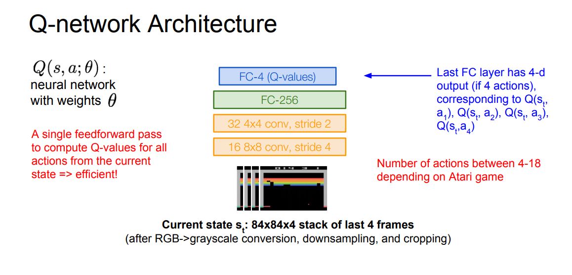
- Q-network Architecture:
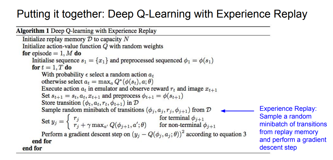
- Learning from batches of consecutive samples is a problem. If we recorded a training data and set the NN to work with it, if the data aren’t enough we will go to a high bias error. so we should use “experience replay” instead of consecutive samples where the NN will try the game again and again until it masters it.
- Continually update a replay memory table of transitions (
s[t],a[t],r[t],s[t+1]) as game (experience) episodes are played. - Train Q-network on random minibatches of transitions from the replay memory, instead of consecutive samples.
- The full algorithm:
- A video that demonstrate the algorithm on Atari game can be found here: “https://www.youtube.com/watch?v=V1eYniJ0Rnk”
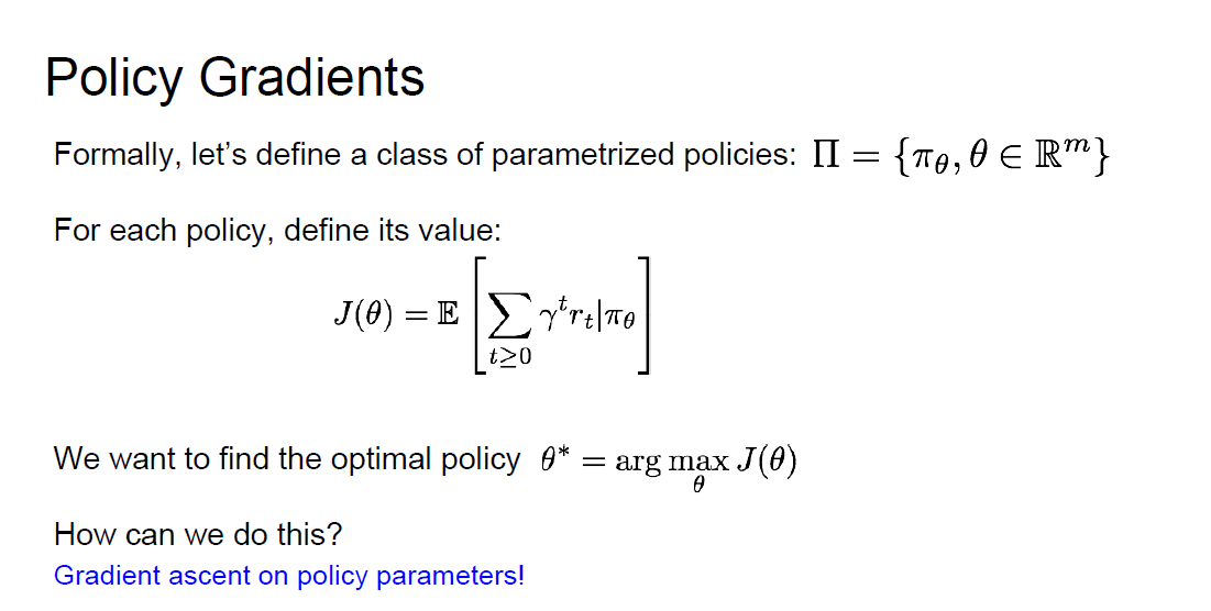
- Policy Gradients
- The second deep learning algorithm that solves the RL.
- The problem with Q-function is that the Q-function can be very complicated.
- Example: a robot grasping an object has a very high-dimensional state.
- But the policy can be much simpler: just close your hand.
- Can we learn a policy directly, e.g. finding the best policy from a collection of policies?
- Policy Gradients equations:
- Converges to a local minima of
J(ceta), often good enough! - REINFORCE algorithm is the algorithm that will get/predict us the best policy
- Equation and intuition of the Reinforce algorithm:
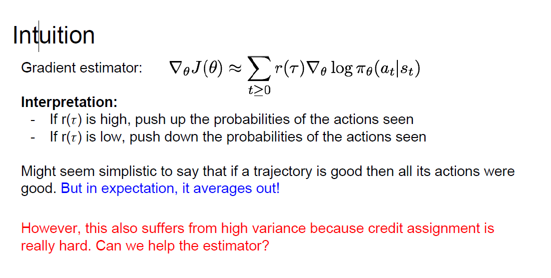
- the problem was high variance with this equation can we solve this?
- variance reduction is an active research area!
- Recurrent Attention Model (RAM) is an algorithm that are based on REINFORCE algorithm and is used for image classification problems:
- Take a sequence of “glimpses” selectively focusing on regions of the image, to predict class
- Inspiration from human perception and eye movements.
- Saves computational resources => scalability
- If an image with high resolution you can save a lot of computations
- Able to ignore clutter / irrelevant parts of image
- RAM is used now in a lot of tasks: including fine-grained image recognition, image captioning, and visual question-answering
- Take a sequence of “glimpses” selectively focusing on regions of the image, to predict class
- AlphaGo are using a mix of supervised learning and reinforcement learning, It also using policy gradients.
- A good course from Standford on deep reinforcement learning
- http://web.stanford.edu/class/cs234/index.html
- https://www.youtube.com/playlist?list=PLkFD6_40KJIwTmSbCv9OVJB3YaO4sFwkX
- A good course on deep reinforcement learning (2017)
- http://rll.berkeley.edu/deeprlcourse/
- https://www.youtube.com/playlist?list=PLkFD6_40KJIznC9CDbVTjAF2oyt8_VAe3
- A good article
- https://www.kdnuggets.com/2017/09/5-ways-get-started-reinforcement-learning.html
Further Reading
Here are some (optional) links you may find interesting for further reading:
- Receptive field to learn about the concept of receptive field and effective receptive field.
- Introduction to t-SNE to learn implementation details about t-SNE.
- Adversarial Examples and Adversarial Training to learn more about this adversarial training and examples.
Citation
If you found our work useful, please cite it as:
@article{Chadha2020DistilledDeepReinforcementLearning,
  title   = {Deep Reinforcement Learning},
  author  = {Chadha, Aman},
  journal = {Distilled Notes for Stanford CS231n: Convolutional Neural Networks for Visual Recognition},
  year    = {2020",
  note    = {\url{https://aman.ai}}
}