CS231n • Neural Networks and Backpropagation
Overview
-
At their core, neural networks are functions that transform inputs into outputs through a sequence of mathematical operations. A simple linear model has the form
\[f(x; W) = W x,\]- where \(x\) is the input and \(W\) is a weight matrix. While linear functions are powerful in some contexts, they are fundamentally limited: they cannot capture complex, nonlinear relationships.
-
To overcome this limitation, neural networks introduce nonlinearities between layers of linear transformations. For example, a two-layer neural network can be written as:
\[f(x; W_1, W_2) = W_2 \, \max(0, W_1 x),\]- where the function \(\max(0, \cdot)\) is the Rectified Linear Unit (ReLU) activation (Nair & Hinton, 2010), the most commonly used nonlinearity in modern deep learning. Nonlinearities allow neural networks to approximate highly complex functions, going far beyond what linear models can capture.
-
Without the nonlinearity, the model would collapse back to a single linear transformation:
\[f(x; W_1, W_2) = (W_2 W_1) x,\]- which is equivalent to a one-layer linear model with combined weights. Thus, nonlinearities are the essential ingredient that make neural networks expressive.
Hidden Layers and Depth
-
Each additional set of weights corresponds to a new layer. Layers between the input and output are called hidden layers, and the number of hidden layers is referred to as the depth of the network. For instance:
- A 2-layer network has one hidden layer and one output layer.
- A 3-layer network has two hidden layers and one output layer.
-
By increasing the depth and number of neurons per layer, we increase the representational capacity of the model.
Example: CIFAR-10 Network
-
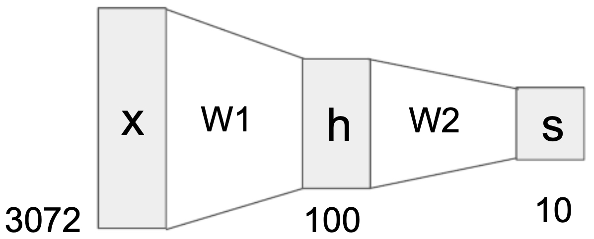
Consider the CIFAR-10 dataset, where each input image is represented as a vector of size 3072 (32 × 32 × 3). If we design a two-layer neural network with a hidden layer of 100 neurons and an output layer of 10 neurons (corresponding to the 10 classes), then:
- \(W_1 \in \mathbb{R}^{100 \times 3072}\) maps the input to the hidden layer,
- \(W_2 \in \mathbb{R}^{10 \times 100}\) maps hidden features to class scores.
-
The following figure shows the structure of a 2-layer neural network for CIFAR-10, where the input vector is mapped to 100 hidden neurons, and then to 10 class outputs.
Computational Graphs
-
Neural networks can be understood in terms of computational graphs, which are directed acyclic graphs where nodes represent mathematical operations (addition, multiplication, activation functions, etc.), and edges represent the flow of data (scalars, vectors, or tensors). This perspective provides a structured and visual way to represent both the forward pass (computing outputs) and the backward pass (computing gradients).
-
Computational graphs are extremely useful because they enable automatic differentiation. Modern deep learning frameworks such as TensorFlow and PyTorch build these graphs internally, storing intermediate values during the forward pass and then applying the chain rule of calculus during the backward pass to compute gradients efficiently.
Hinge Loss as a Computational Graph
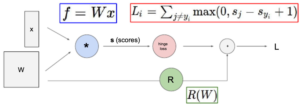
- To illustrate, consider the hinge loss function, commonly used in classification tasks. Given an input vector \(x\), class scores are computed as
- where \(W\) is the weight matrix. The hinge loss for a training example is then:
-
where \(s_y\) is the score for the correct class, \(s_j\) is the score of an incorrect class, and \(R(W)\) is a regularization term that penalizes large weights.
-
This loss can be decomposed into a series of primitive operations—matrix multiplication, subtraction, maximum, and addition—that naturally form a computational graph. Each node in the graph computes a local operation, and together they define the overall function.
-
The following figure illustrates how the hinge loss calculation can be represented as a computational graph, highlighting how scores are computed, passed through the hinge loss, and then combined with the regularization term.. Note that this representation is not unique: multiple computational graphs could represent the same function, depending on how we expand the operations.
Backpropagation
-
Backpropagation is the algorithm that enables efficient training of neural networks by systematically applying the chain rule of calculus across computational graphs (Rumelhart, Hinton & Williams, 1986). While often described as a separate algorithm, backpropagation is simply a way to compute gradients of a complex function expressed as a graph.
-
The process involves two passes:
- Forward pass: The network computes outputs layer by layer, storing intermediate results at each node.
- Backward pass: Starting from the final loss, gradients are propagated backward through the graph by multiplying local gradients (derivatives of each operation) with upstream gradients (coming from later nodes).
-
This modular design allows us to scale the method across very deep and complex networks, as each node only needs information from its immediate neighbors.
A Simple Example
-
Consider the function
\[f(x, y, z) = (x + y)z, \quad q = x + y.\] -
In the forward pass, we compute:
- \[q = x + y\]
- \[f = qz\]
-
In the backward pass, derivatives are calculated as:
-
This demonstrates how backpropagation distributes derivatives across multiple inputs using the chain rule.
-
The following figure shows the computational graph for this example with both forward values (green) and backward gradients (red).
Local and Upstream Gradients
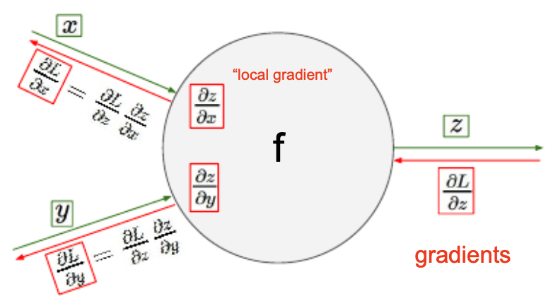
- Backpropagation generalizes by combining local gradients with upstream gradients. Suppose a node computes \(z = g(x)\), and the upstream gradient is \(\frac{\partial f}{\partial z}\). Then:
-
This means each node only requires information from its neighbors to compute the gradient, which makes the process scalable across large graphs.
-
The following figure shows how, during both forward and backward passes, each node’s computation depends only on its local neighbors.
Worked Numerical Example
-
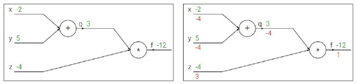
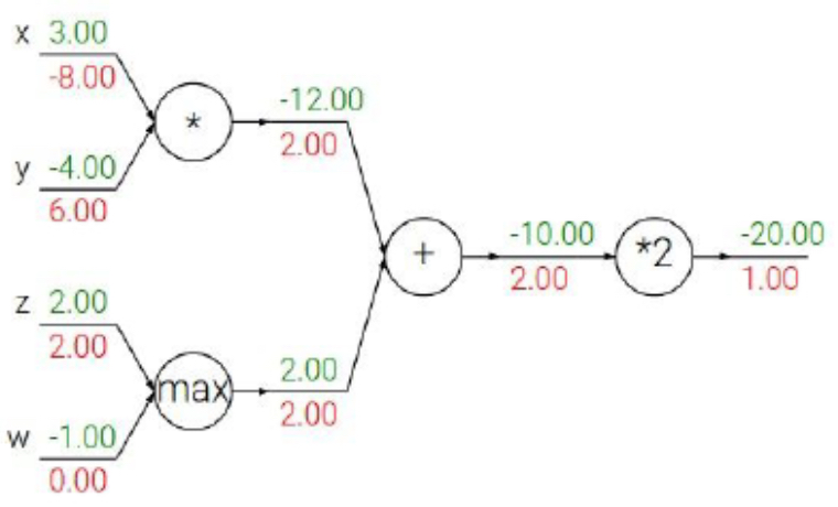
To illustrate a more concrete case, let us evaluate the function \(f(x,y,z) = (x+y)z\), with specific values: \(x = 2, y = 5, z = 4\).
-
Forward pass:
- \[q = x + y = 2 + 5 = 7\]
- \[f = qz = 7 \cdot 4 = 28\]
-
Backward pass:
- \[\frac{\partial f}{\partial z} = q = 7\]
- \[\frac{\partial f}{\partial x} = z = 4\]
- \[\frac{\partial f}{\partial y} = z = 4\]
-
The following figure shows this worked-out computational graph with explicit values in green (forward) and derivatives in red (backward).
A Logistic (Sigmoid) Example
-
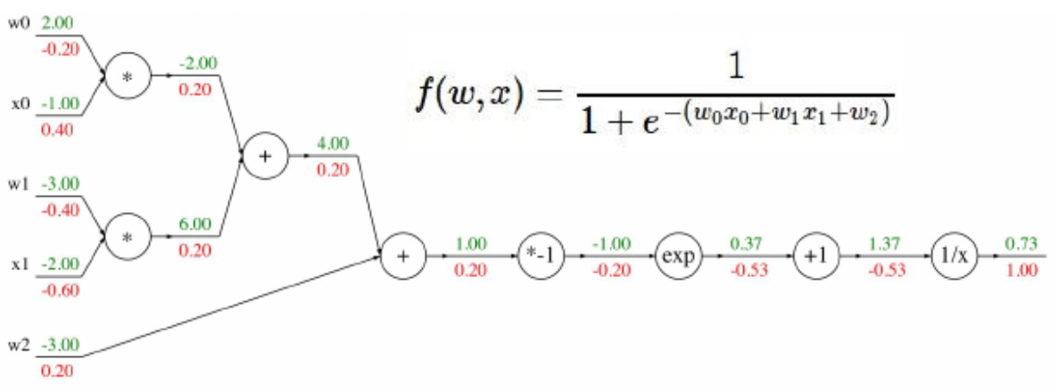
For more complex nonlinear functions such as the logistic sigmoid, backpropagation proceeds in the same modular fashion. Consider \(f(w, x) = \frac{1}{1 + e^{-(w_0 x_0 + w_1 x_1 + w_2)}}\) with initial values:
- \[w_0 = 2, \; x_0 = 1\]
- \[w_1 = 3, \; x_1 = 2\]
- \[w_2 = 3\]
-
The computation graph first evaluates the linear combination, then applies the exponential, addition, reciprocal, and finally the sigmoid. At each step, local derivatives are calculated and multiplied backward via the chain rule. This avoids needing a closed-form derivative of the entire function.
-
The following figure shows the computational graph for the sigmoid example, with forward values in green and backward gradients in red.
Common Backpropagation Gates
-
Many operations in neural networks reduce to a small set of primitive gates with well-known derivative rules:
- Addition gate: distributes gradient equally to each input.
- Multiplication gate: gradient flows proportionally to the other input.
- Max gate: passes gradient to the larger input, zero to the smaller one.
-
The following figure shows how inputs to max, multiply, and addition gates affect both forward output and backward gradients.
Branching in Backpropagation
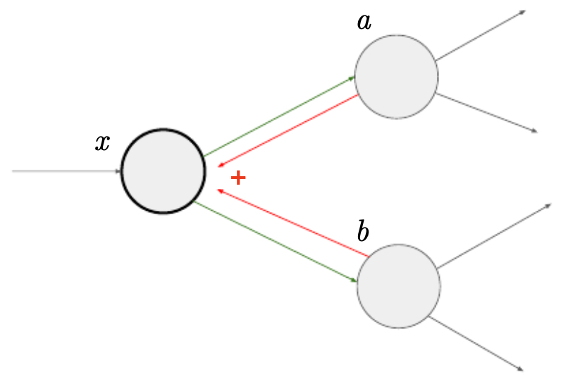
- Sometimes a single input branches into multiple functions. Suppose an input \(x\) is used in two downstream functions \(a(x)\) and \(b(x)\). If both affect final output \(f\), then by the multivariate chain rule:
- The following figure illustrates how an input branching into two functions requires summing contributions from each branch during gradient flow.
Vectorized Backpropagation
- In practice, networks operate on vectors, matrices, and tensors. Gradients generalize to Jacobians. For a function \(f: \mathbb{R}^n \to \mathbb{R}^m\), the Jacobian is:
-
During backpropagation, the upstream gradient (a vector) is multiplied by this Jacobian to yield the downstream gradient. This makes the process compatible with high-dimensional data such as images and sequences.
-
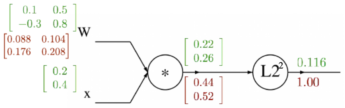
The following figure shows the computational graph for a quadratic form \(f(W, x) = \lVert W x \rVert_2^2\), demonstrating vectorized backpropagation.
Modular Implementations
-
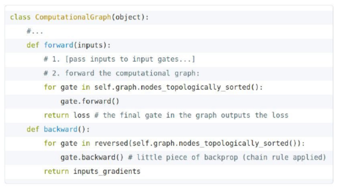
Modern frameworks implement backpropagation modularly, with explicit forward and backward passes defined per node or layer. For example:
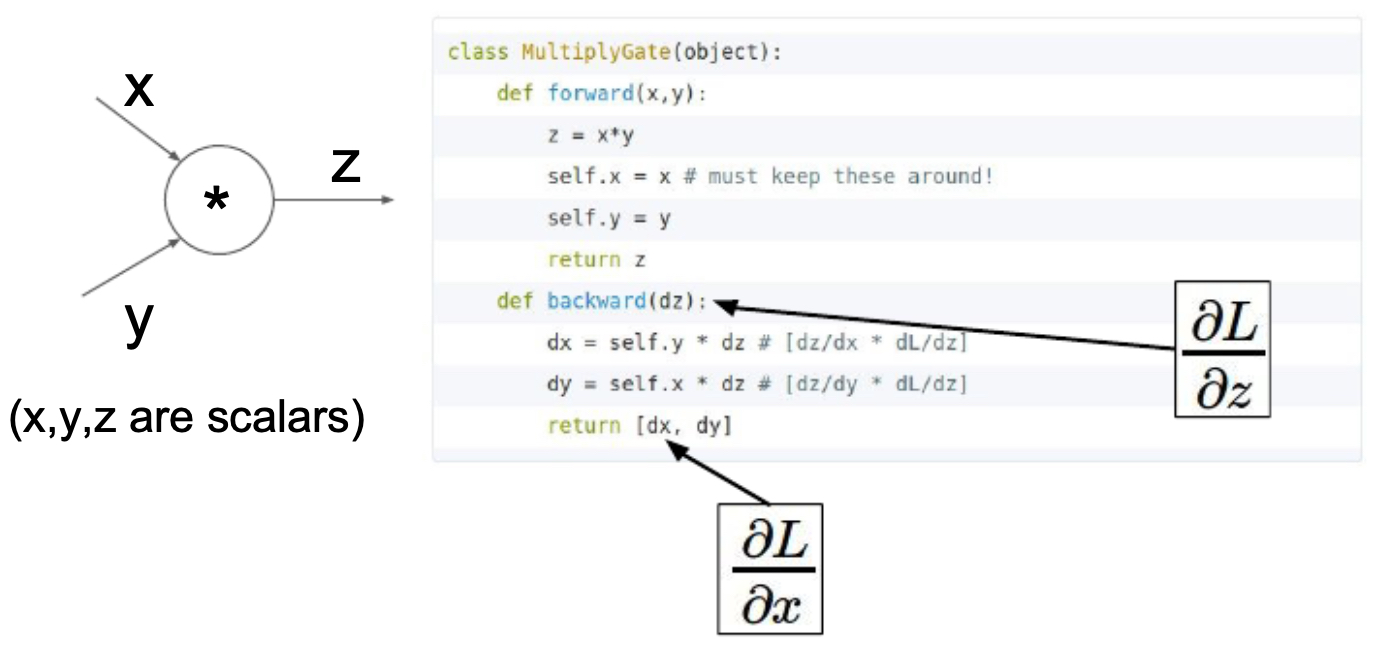
- Multiplication gate: defines both forward computation and gradient rules.
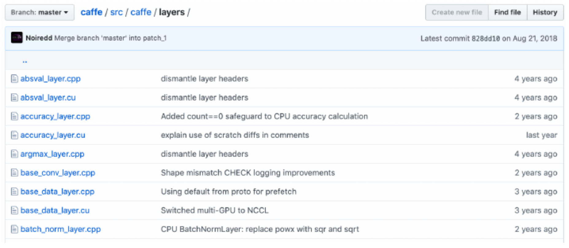
- Caffe framework: defines each layer (e.g., convolution, sigmoid) as a class with forward and backward functions.
-
The following figure shows pseudocode for a modularized computational-graph class.
- The following figure shows a multiplication gate implementation with forward and backward functions.
- The following figure shows several layers available in the Caffe deep learning framework, each with built-in forward/backward logic.
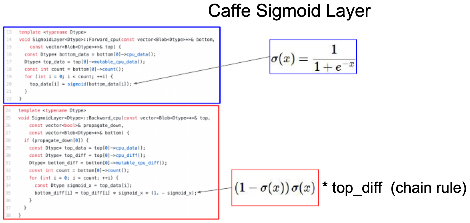
- The following figure shows the Sigmoid layer implementation in Caffe, with explicit forward and backward computations.
Backpropagation in a Neuron
-
At the level of a single neuron, the forward pass computes:
\[s = w^T x + b, \quad y = f(s),\]- where \(w\) is the weight vector, \(x\) the input, \(b\) the bias, and \(f\) a nonlinear activation (e.g., sigmoid, ReLU).
-
In the backward pass, gradients flow with respect to \(w\), \(b\), and \(x\), ensuring that each parameter can be updated through gradient descent.
Types of Neural Networks
- Neural networks come in a variety of architectures, each designed to exploit the structure of different types of data. While the foundation of feedforward computation remains the same, architectural variations determine their effectiveness across tasks such as image classification, sequential modeling, and natural language understanding.
Feedforward Neural Networks (FNNs)
-
The simplest neural network is the feedforward neural network (FNN), where data flows in a single direction: from input, through hidden layers, to output. These consist of affine transformations followed by nonlinear activation functions. Despite their simplicity, FNNs are powerful: the Universal Approximation Theorem guarantees that they can approximate any continuous function given sufficient hidden units.
-
However, without nonlinear activation functions, stacked linear layers collapse into a single linear transformation:
\[f(W) = W_2 \cdot (W_1 x) = (W_2 W_1) x,\]- which is no more expressive than a single linear layer. Nonlinearities such as ReLU (Rectified Linear Unit) Nair & Hinton, 2010 enable networks to capture complex decision boundaries.
-
The following figure shows a schematic of a simple feedforward neural network.
Connection to the Brain
-
Neural networks derive their name from their loose analogy to biological neurons. Although artificial neurons are much simpler than real ones, the analogy provides historical context and intuition.
-
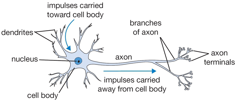
In a biological neuron:
- Dendrites receive signals from other neurons.
- The cell body integrates these signals.
- If the combined signal exceeds a threshold, the neuron fires, sending an electrical impulse through the axon to downstream neurons.
- The axon branches into synaptic terminals, which transmit signals to other neurons.
-
The following figure shows a labeled schematic of a biological neuron with dendrites, cell body, axon, and synaptic terminals.
-
Artificial neurons mimic this behavior:
- Weights act like dendrites, aggregating inputs.
- The activation function acts like the cell body, deciding whether the neuron “fires.”
- The output corresponds to the axon transmitting the signal forward.
-
The following figure illustrates this comparison between parts of a biological neuron and components of an artificial neural network.
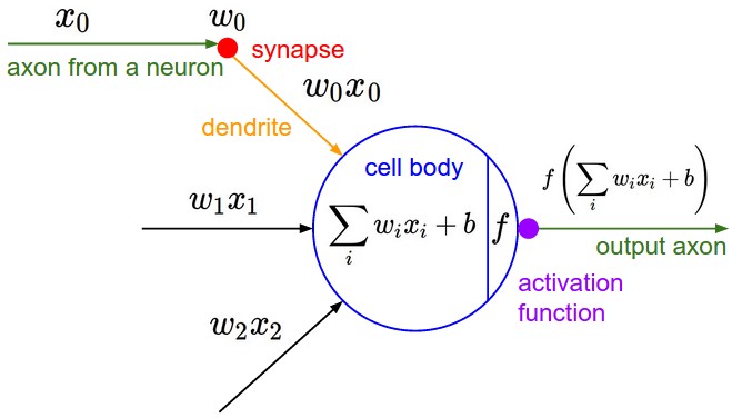
- More broadly, modern networks diverge significantly from biology. Biological neurons can perform highly nonlinear computations even within their dendrites London & Häusser, 2005. Thus, while the analogy is instructive, artificial neural networks are best viewed as flexible mathematical function approximators rather than strict biological models.
Computational Graph Perspective
- Another perspective is to view neural networks directly as computational graphs, where nodes represent operations and edges carry activations. This lens emphasizes modularity, making it straightforward to connect architectures to backpropagation.
Convolutional Neural Networks (CNNs)
-
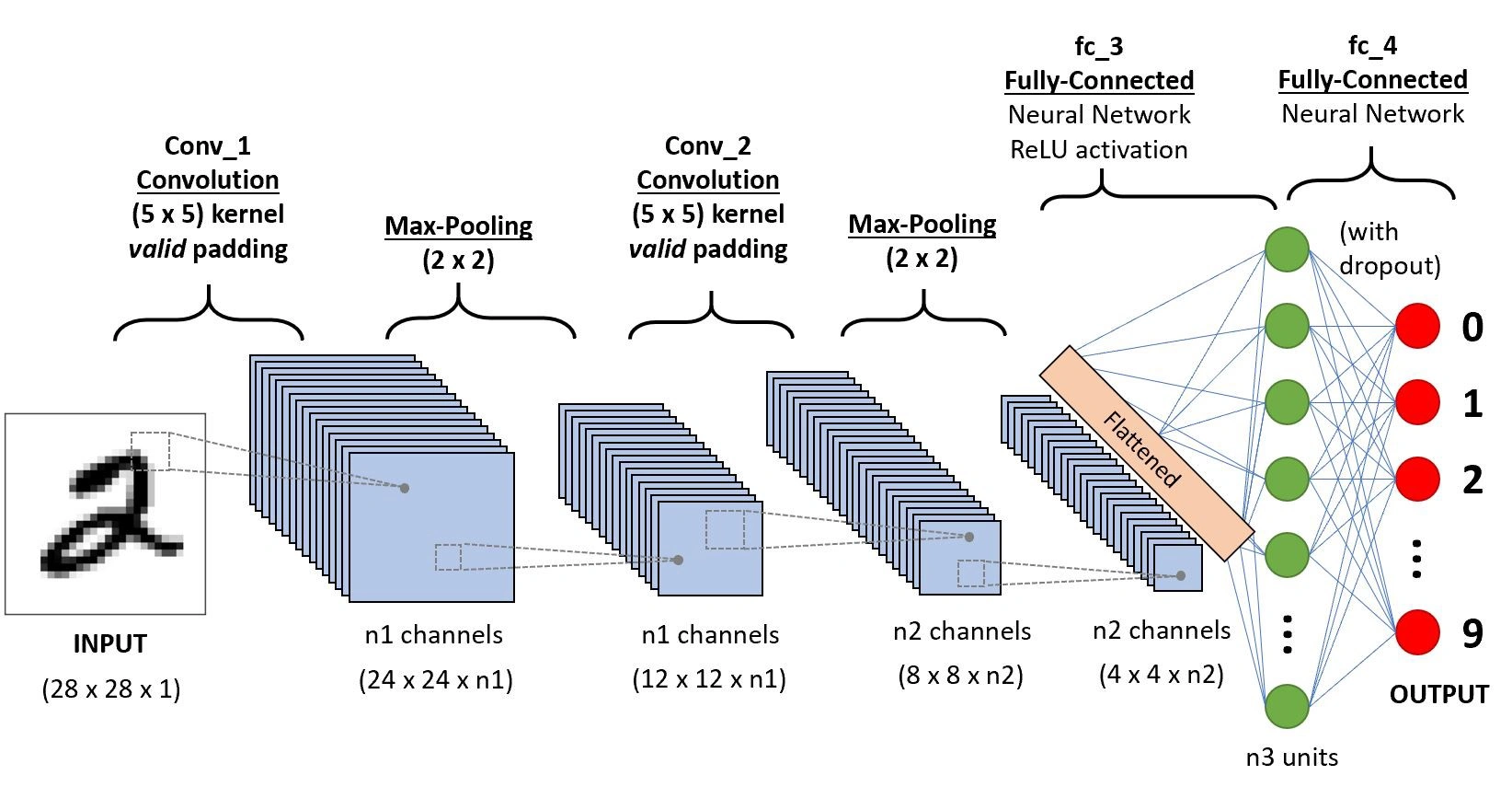
For image data, which has a grid-like spatial structure, Convolutional Neural Networks (CNNs) are the dominant architecture. They leverage:
- Convolutional layers: Learn spatially localized filters that detect edges, textures, and higher-level features.
- Pooling layers: Downsample feature maps, reducing spatial resolution while preserving salient information.
- Fully connected layers: Aggregate high-level features into final predictions.
-
CNNs exploit weight sharing, making them computationally efficient and translation-invariant. Their success was highlighted in the landmark ImageNet result by Krizhevsky et al., 2012.
-
The following figure shows a generic CNN architecture, with convolutional, pooling, and fully connected stages.
Recurrent Neural Networks (RNNs)
-
For sequential data such as text, audio, or time-series, Recurrent Neural Networks (RNNs) are designed to handle temporal dependencies. They introduce cycles in their connections, allowing hidden states to persist over time. At time step \(t\), the hidden state is updated as:
\[h_t = f(W_{hh} h_{t-1} + W_{xh} x_t + b_h),\]- where \(h_t\) is the hidden state, \(x_t\) the input at time \(t\), and \(f\) a nonlinearity (e.g., sigmoid, tanh, or ReLU). This recurrence allows information to flow across time, enabling modeling of dependencies spanning multiple steps. However, RNNs are prone to vanishing and exploding gradients, which limit their ability to model long sequences (a problem partially solved by LSTMs and GRUs).
-
The following figure shows an unfolded RNN, where the same weights are reused across time steps to process sequences.

Word Embeddings
-
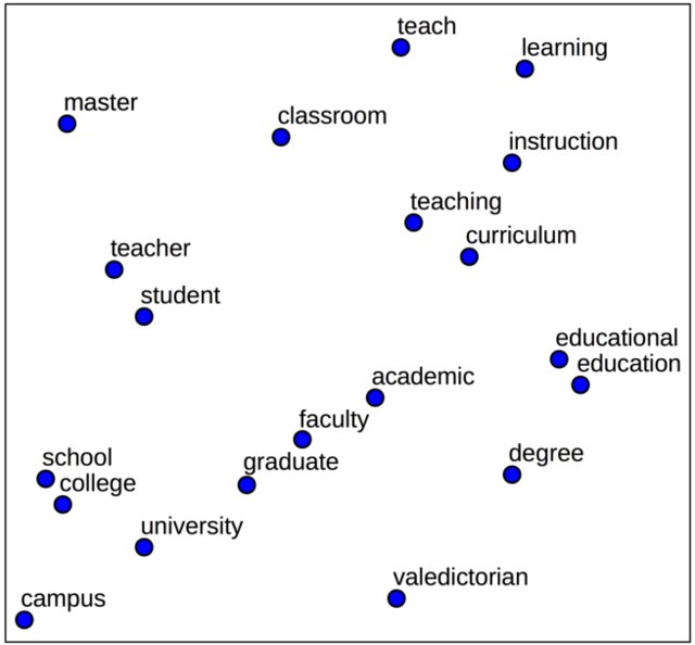
In natural language processing, raw words cannot be directly fed into networks. Instead, they are mapped to word embeddings, which represent words in continuous vector spaces where semantic similarity corresponds to geometric proximity.
-
Models such as Word2Vec (Mikolov et al., 2013) and GloVe (Pennington et al., 2014) learn embeddings that capture meaningful relationships. For example:
- The following figure shows a 2D projection of embeddings, where semantically related words cluster together.
Citation
If you found our work useful, please cite it as:
@article{Chadha2020NeuralNetworksAndBackpropagation,
  title   = {Neural Networks and Backpropagation},
  author  = {Chadha, Aman},
  journal = {Distilled Notes for Stanford CS231n: Convolutional Neural Networks for Visual Recognition},
  year    = {2020},
  note    = {\url{https://aman.ai}}
}