CS231n • Loss Functions
- Overview
- Why is the loss function important?
- Binary Classifier (Logistic Regression)
- Softmax Classifier (Multinomial Logistic Regression)
- Multiclass SVM Loss (“Hinge Loss”)
- Comparing SVM and Softmax
- Regularization
- Optimization
- Gradient Descent Variants
- The Optimization Loop
- Citation
Overview
-
A loss function, sometimes referred to as a cost function or objective function, is the cornerstone of nearly all machine learning algorithms. It provides a quantitative measure of how wrong a model’s predictions are compared to the true outcomes. Without a loss function, there is no way to guide the training process, since the model would not know how to adjust its parameters to improve performance.
-
In supervised learning, the goal is to learn a mapping from inputs to outputs. Suppose we are training a classifier on a dataset of images. Each training example consists of an input image, denoted by \(x_i\), and its corresponding ground-truth label, denoted by \(y_i\). The model, parameterized by weights \(W\) and biases \(b\), produces a vector of scores:
\[s = f(x_i; W, b)\]- where \(s\) is a vector of raw scores (sometimes called logits), one for each possible class. The loss function then compares these predicted scores against the true label \(y_i\).
-
Formally, for a dataset with \(N\) examples, the overall loss is defined as the average of the individual per-example losses:
\[L = \frac{1}{N} \sum_{i=1}^N L_i(f(x_i; W, b), y_i)\]-
where:
- \(L_i\) represents the loss for a single training example.
- \(f(x_i; W, b)\) are the scores (or probabilities) the model produces for input \(x_i\).
- The summation averages across all training samples, ensuring that the loss does not scale with dataset size.
-
-
This average loss, often called the empirical risk, is the value that optimization algorithms attempt to minimize during training (Vapnik, 1998).
-
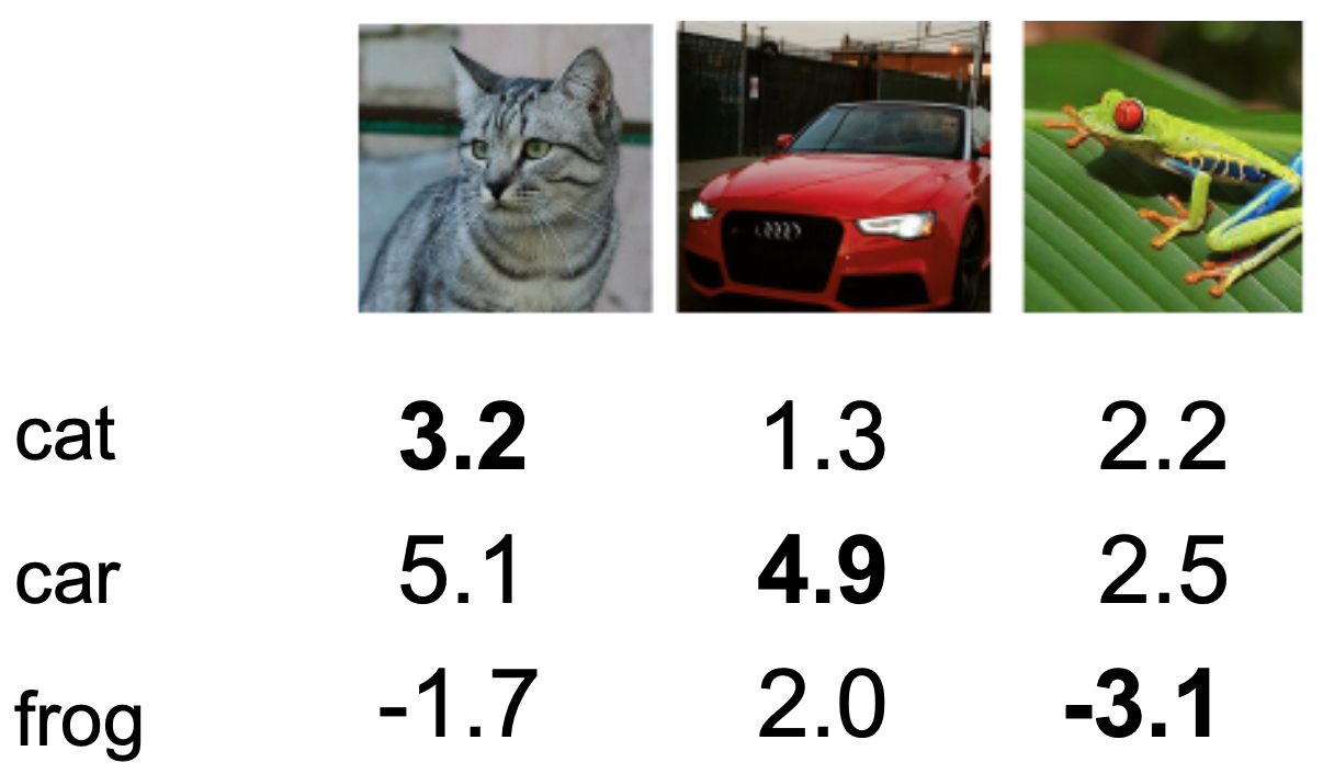
The following figure illustrates an example of the raw scores produced by a linear classifier for three classes (cat, car, frog). Each entry corresponds to the unnormalized score for a class, and the loss function will ensure that the score for the correct class is maximized while the others are minimized.
Why is the loss function important?
- The loss function is central because it translates model performance into a numerical value that can be optimized. Without it, learning would be unguided. Its importance can be broken down into several dimensions:
Guides optimization
- The loss function provides a direction for gradient-based optimization. Gradients are computed with respect to the loss, and these gradients tell us how to update weights \(W\) and biases \(b\).
- Instead of searching randomly through possible parameter configurations — which would be infeasible in high-dimensional spaces with millions of parameters — the loss function acts like a landscape, guiding the optimization process downhill toward better models (Cauchy, 1847).
Encodes model goals
-
The choice of loss function reflects what we care about:
- Regression tasks: Mean Squared Error (MSE) (Gauss, 1821).
- Classification tasks: Cross-Entropy (Shannon, 1948) or Hinge loss (Cortes & Vapnik, 1995).
-
Structured outputs: More specialized losses may be used for ranking, segmentation, or translation.
-
Different loss functions induce different training dynamics and learning behaviors. For example, hinge loss enforces margins, while cross-entropy encourages probabilistic confidence.
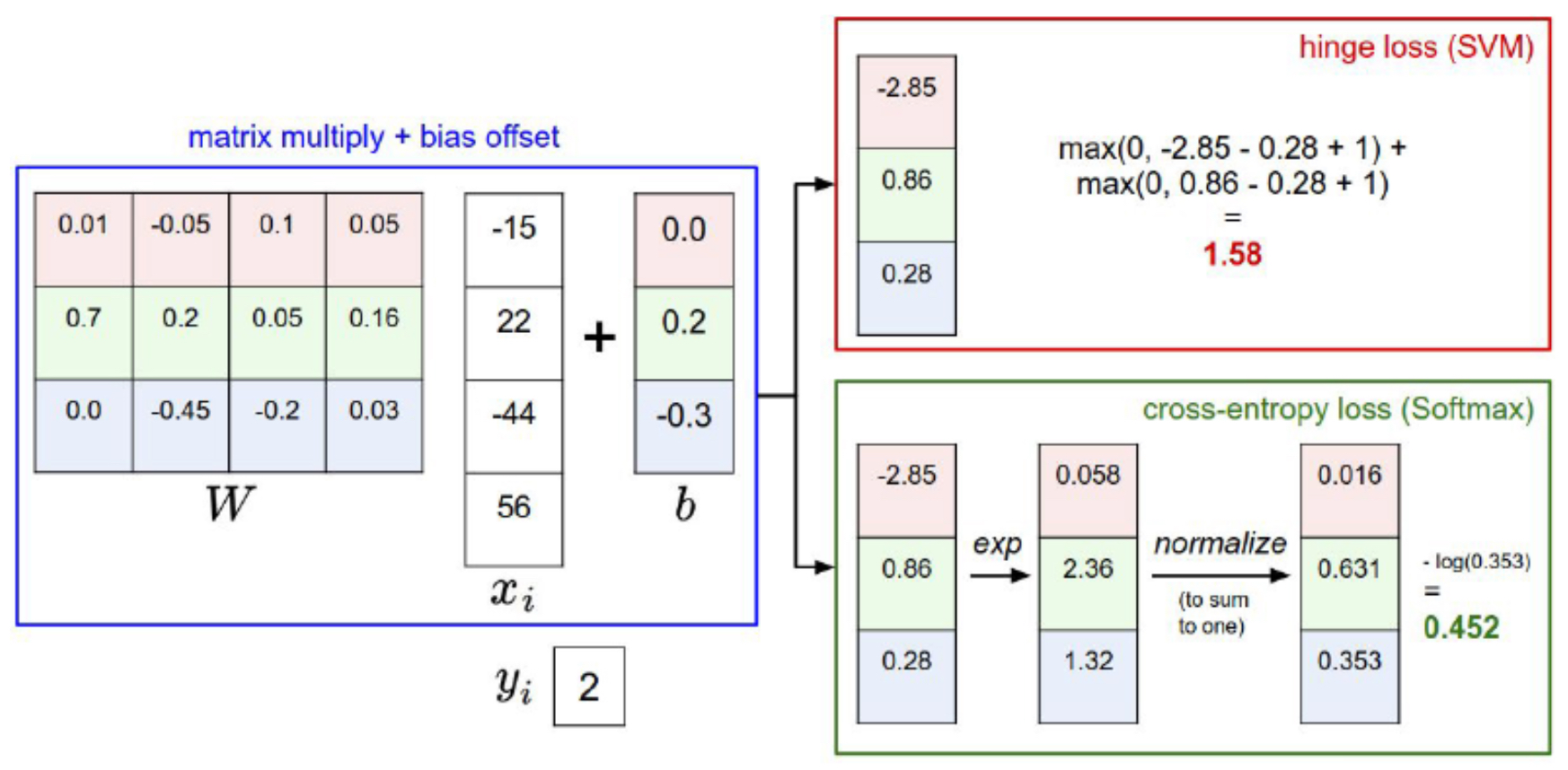
- The following figure illustrates how different loss formulations interpret and act on the scores of correct and incorrect classes. While hinge loss focuses on enforcing a margin, cross-entropy loss continues to push probabilities closer to certainty, even if the correct class is already higher.
Balances accuracy vs. generalization
-
Loss functions can include not only data loss (how well we fit the training set) but also regularization penalties, which encourage simpler models that generalize better (Tikhonov, 1963).
-
This reflects Occam’s Razor — the principle that, among competing hypotheses, the simplest is often best. By penalizing overly complex models (e.g., with L2 or L1 regularization), we prevent overfitting while retaining explanatory power.
Key takeaway
- Loss functions are not arbitrary; they are design choices that encode what “success” means for a model. A poorly chosen loss can misalign optimization with the actual task, while the right one ensures learning progresses efficiently and meaningfully.
Binary Classifier (Logistic Regression)
-
Before diving into multiclass settings such as SVM or Softmax, it is useful to first study the binary classification problem, where there are only two possible outcomes (e.g., “cat” vs. “not cat”). Many of the principles in multiclass classification extend from this simpler case.
-
In binary classification, we typically assign labels as \(y_i \in \{0, 1\}\) or equivalently \(y_i \in \{-1, +1\}\). Given an input \(x_i\), the model predicts a scalar score:
- This score is then mapped to a probability that the input belongs to the positive class.
Logistic Regression Model
-
The most common binary classifier is Logistic Regression (Cox, 1958). Logistic regression models the conditional probability of class membership using the sigmoid (logistic) function:
\[P(Y = 1 \mid X = x_i) = \sigma(s) = \frac{1}{1 + e^{-s}}\]-
where:
- \(s = W^T x_i + b\) is the linear score.
- The sigmoid squashes any real-valued score into the interval \((0, 1)\), making it interpretable as a probability.
-
-
If \(P(Y=1 \mid X=x_i) > 0.5\), the model predicts the positive class; otherwise, it predicts the negative class.
Loss Function: Binary Cross-Entropy
- To train logistic regression, we minimize the Binary Cross-Entropy loss (also called Log Loss) (Shannon, 1948):
-
Interpretation:
- If \(y_i = 1\), the loss reduces to \(-\log(\sigma(s))\), penalizing the model if the predicted probability of the positive class is low.
- If \(y_i = 0\), the loss reduces to \(-\log(1 - \sigma(s))\), penalizing the model if the predicted probability of the negative class is low.
- The loss is minimized when the predicted probability matches the true label.
-
For a dataset of \(N\) examples, the total loss is the average:
Geometric View
-
Logistic regression learns a linear decision boundary between the two classes:
\[W^T x + b = 0\]- The weights \(W\) define the orientation of the boundary.
- The bias \(b\) shifts it.
- The sigmoid ensures that confidence grows smoothly as points move farther from the boundary.
-
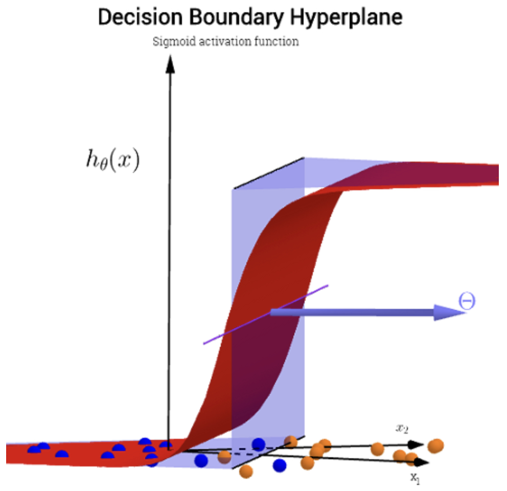
The following figure (source) shows how a linear decision boundary separates two classes in a 2D feature space, and how the sigmoid transitions scores into probabilities.
Worked Example
-
Suppose we want to classify emails as spam (\(y=1\)) or not spam (\(y=0\)) using features like word frequency. If the score for an email is \(s=2.0\):
-
Predicted probability: \(\sigma(2.0) = \frac{1}{1+e^{-2}} \approx 0.88\)
-
If \(y=1\) (spam), loss = \(-\log(0.88) \approx 0.13\) (good prediction).
-
If \(y=0\) (not spam), loss = \(-\log(1 - 0.88) \approx 2.13\) (bad prediction).
-
Key Properties
- Probabilistic interpretation: Logistic regression directly models \(P(Y \mid X)\), which is useful for applications requiring uncertainty estimates.
- Convex optimization: The binary cross-entropy loss is convex in \(W, b\), ensuring global optima can be found efficiently with gradient descent.
- Simplicity and interpretability: Each weight in \(W\) indicates how strongly a feature contributes to predicting the positive class.
- Limitations: The linear decision boundary restricts its expressiveness; it cannot separate classes that are not linearly separable. Extensions like polynomial features or kernels can address this.
Softmax Classifier (Multinomial Logistic Regression)
-
The Softmax classifier offers a fundamentally different perspective from hinge loss. While SVM loss enforces a margin-based separation, the Softmax classifier interprets scores in a probabilistic framework (Bishop, 2006), providing outputs that can be directly interpreted as probabilities. This makes it especially attractive in tasks where calibrated confidence estimates are important.
-
The idea is to take the unbounded raw scores (logits) produced by the model, and transform them into a normalized probability distribution over all possible classes.
The Softmax Function
- Given a score vector \(s = f(x_i; W, b)\) for input \(x_i\), the probability that the input belongs to class \(k\) is:
- The numerator exponentiates the raw score of class \(k\). Larger scores yield larger exponentials, making high-scoring classes more dominant.
- The denominator sums over exponentials of all class scores, ensuring the output probabilities are normalized and sum to 1.
-
The transformation is smooth and differentiable, making it ideal for gradient-based optimization.
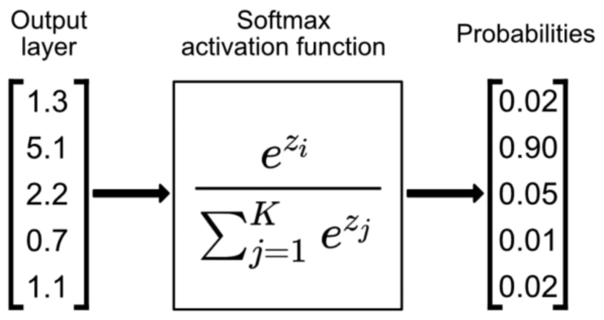
- The following figure (source) illustrates how raw class scores are transformed into normalized probabilities using Softmax.
Cross-Entropy Loss
- To train the Softmax classifier, we use the Cross-Entropy Loss, which compares the predicted probability distribution with the true distribution. For a single example, where the correct class is \(y_i\):
-
This can be rewritten as:
\[L_i = -s_{y_i} + \log \left( \sum_j e^{s_j} \right)\]-
where:
- The first term penalizes the model if the score of the correct class is low.
- The second term ensures normalization and prevents trivial solutions where all scores go to negative infinity.
-
-
The loss is minimized when the predicted probability for the correct class approaches 1.
Worked Example
-
Using the example scores from a linear classifier (Cat: 3.2, Car: 5.1, Frog: –1.7):
- Exponentiate each score:
- Compute the sum of exponentials:
- Normalize to probabilities:
- If the true class is Cat, the loss is:
-
This example shows how even though the car class receives a higher score, the cross-entropy loss punishes the model heavily for assigning low probability to the true class.
-
The following figure contrasts how multiclass SVM and Softmax loss respond to scores. SVM loss is flat once the margin is satisfied, while Softmax loss always encourages further probability concentration on the correct class.
Key Properties
- Probabilistic interpretation: Each score is converted into a probability, enabling uncertainty estimates.
- Smooth gradients: Unlike hinge loss, which is piecewise linear, Softmax + Cross-Entropy provides smooth gradients everywhere, which often helps optimization.
- Unbounded confidence drive: The loss decreases as the model pushes \(s_{y_i}\) further above others. Unlike hinge loss, there is no plateau — the model is always incentivized to increase its confidence in the correct class.
- Common in deep learning: Cross-Entropy with Softmax is the standard choice for classification tasks in modern neural networks.
Multiclass SVM Loss (“Hinge Loss”)
-
The Multiclass Support Vector Machine (SVM) loss, commonly known as Hinge loss, is one of the earliest and most influential loss functions for classification tasks (Cortes & Vapnik, 1995).
-
Its central idea is not just to predict the correct class with the highest score, but to do so with a sufficient safety margin. This makes the classifier more robust, since it requires the correct prediction to be confidently separated from incorrect ones.
-
At its core, the hinge loss encourages a decision boundary where the score for the true class is at least a margin \(\Delta\) larger than every incorrect class score. Unlike probabilistic methods (e.g., Softmax), the SVM approach is margin-based, explicitly focusing on geometric separation between classes.
Formal Definition
-
Suppose the model produces a score vector \(s = f(x_i; W, b)\) for input \(x_i\). Let \(s_{y_i}\) denote the score of the true class and \(s_j\) denote the score for an incorrect class \(j\). The multiclass SVM loss for a single training example is:
\[L_i = \sum_{j \ne y_i} \max(0, s_j - s_{y_i} + \Delta)\]-
where:
- The term \(s_j - s_{y_i} + \Delta\) measures how much the incorrect class \(j\) violates the margin requirement.
- If \(s_{y_i} \geq s_j + \Delta\), the margin is satisfied and the contribution to the loss for that class is zero.
- If \(s_{y_i} < s_j + \Delta\), the margin is violated and the loss grows linearly with the violation.
-
-
The margin parameter \(\Delta > 0\) is usually set to 1. It does not drastically affect the final performance but ensures predictions are not only correct, but confidently correct.
-
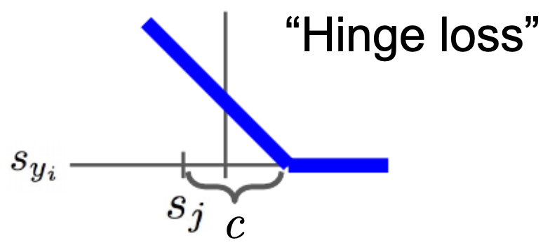
The following figure shows why hinge loss gets its name: the loss curve resembles the shape of a hinge when plotted against the score difference between correct and incorrect classes, i.e., by plotting \(L_i\) as a function of \(s_{y_i}\), parameterized by \(s_j\) and margin \(\Delta\).
Worked Examples
-
Consider the score table below, produced by a linear classifier for three classes: Cat, Car, and Frog.
-
The following figure illustrates arbitrary example scores from a linear classifier across three classes. Each row represents the raw outputs (logits) for a different input.
-
Let’s compute losses with \(\Delta = 1\).
-
Example 1: Cat (correct score: 3.2)
\[L_i = \max(0, 5.1 - 3.2 + 1) + \max(0, -1.7 - 3.2 + 1)\] \[= \max(0, 2.9) + \max(0, -3.9) = 2.9 + 0 = 2.9\] -
Example 2: Car (correct score: 2.2)
\[L_i = \max(0, -3.1 - 2.2 + 1) + \max(0, 2.5 - 2.2 + 1)\] \[= \max(0, -4.3) + \max(0, 1.3) = 0 + 1.3 = 1.3\] -
Example 3: Frog (correct score: 1.3)
\[L_i = \max(0, 4.9 - 1.3 + 1) + \max(0, 2.0 - 1.3 + 1)\] \[= \max(0, 4.6) + \max(0, 1.7) = 6.3\] -
Notice how only the classes that violate the margin contribute to the loss.
Geometric Intuition
-
Hinge loss reflects the geometric principle of SVMs: maximize the margin between the decision boundary and data points.
-
Intuitively, the classifier prefers solutions where data points are not just classified correctly, but are far away from the boundary that separates classes. This reduces sensitivity to noise or small perturbations in the data.
-
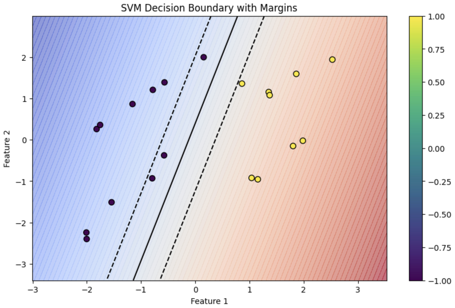
The following figure (source) illustrates the geometric separation enforced by hinge loss. Data points are classified not only correctly but with a buffer zone (the margin) around the boundary.
Python Implementation (Vectorized)
- Here’s a simple vectorized implementation in Python-like pseudocode:
def L_i(x, y, W):
    scores = W.dot(x)
    margins = np.maximum(0, scores - scores[y] + 1)
    margins[y] = 0
    loss_i = np.sum(margins)
    return loss_i
-
This highlights two key facts:
- Many different \(W, b\) combinations may achieve zero hinge loss (scaling invariance).
- Without regularization, the model could overfit — hence why hinge loss is often combined with regularization terms (e.g., L2).
Key Properties
- Zero-loss regions: Once the margin is satisfied, hinge loss is zero — the classifier stops “caring” about further increasing \(s_{y_i}\).
- Piecewise linearity: The loss increases linearly when the margin is violated, creating simple gradients for optimization.
- Robustness: By demanding confident predictions, hinge loss reduces the risk of misclassification under small perturbations.
Comparing SVM and Softmax
-
Both the Multiclass SVM loss (hinge loss) and the Softmax loss (cross-entropy) are widely used for classification. At first glance, they may appear quite different: one is rooted in geometric margins, while the other is grounded in probability theory. However, both ultimately encourage the model to assign higher scores to the correct class and lower scores to incorrect ones. The key lies in how they enforce this preference.
-
The following figure illustrates how the loss is calculated under the multiclass SVM formulation compared to the Softmax formulation. While SVM loss flattens out once the margin requirement is satisfied, Softmax loss continues to push probabilities closer to certainty in the process of aiming to maximize the likelihood of the correct class.
Conceptual Difference
-
SVM Loss (Margin-Based Objective): The multiclass hinge loss enforces that the correct class score \(s_{y_i}\) is at least \(\Delta\) higher than every incorrect score \(s_j\). Once this margin requirement is satisfied, the loss becomes zero. In other words, hinge loss focuses on relative separation and stops caring about absolute magnitudes beyond the margin.
-
Softmax Loss (Probability-Based Objective): The cross-entropy loss never reaches zero unless the predicted probability of the correct class is exactly 1. It encourages the model to continually increase \(s_{y_i}\) relative to the others, making the predicted probability of the correct class approach 1. This leads to stronger incentives for confidence maximization.
Visual Analogy
-
Imagine a race between athletes (the classes):
- The SVM says: “As long as my favorite athlete is ahead of everyone else by at least \(\Delta\) seconds, I am satisfied and will not push them to run faster.”
- The Softmax says: “I always want my favorite athlete to be faster than everyone else — the bigger the gap, the happier I am. There is no upper limit to my encouragement.”
Practical Implications
-
SVM Loss:
- Good at ensuring clear decision boundaries.
- Robust once the margin is satisfied (no incentive to over-optimize).
- Can be less smooth for optimization since its gradient is piecewise.
-
Softmax Loss:
- Produces calibrated probabilities that can be interpreted as confidence scores.
- Encourages continual improvement of correct class scores.
- Smooth and differentiable everywhere, which generally helps optimization with gradient-based methods.
Performance in Practice
-
Despite their theoretical differences, both SVM and Softmax classifiers often yield very similar performance on real-world tasks. This is because both losses push the model in the same general direction: to increase \(s_{y_i}\) relative to other scores.
-
However, Softmax loss has become the default choice in deep learning, mainly because:
- It provides probabilistic outputs.
- Its smooth gradient makes optimization easier.
- It integrates seamlessly into neural networks where probabilities are required (e.g., language models, image classifiers).
-
SVM losses, while historically important, are less common in modern deep learning pipelines but remain conceptually useful and are still applied in certain margin-based contexts such as structured prediction.
Regularization
-
In machine learning, there is always a tension between fitting the training data perfectly and generalizing to unseen data. A model with too much capacity can memorize the training set, achieving very low training loss but failing to perform well on new inputs — a phenomenon called overfitting.
-
Regularization provides a systematic way to combat overfitting by penalizing overly complex models. This idea resonates with Occam’s Razor (William of Ockham, 1300s): “Among competing hypotheses, the simplest is the best.”
Regularized Loss Function
- The general form of a regularized loss function is:
- The data loss (first term) measures how well the model fits the training data.
- The regularization loss (second term) penalizes the complexity of the model.
-
\(\lambda\) is a hyperparameter that controls the trade-off:
- Large \(\lambda\) emphasizes regularization, possibly underfitting the data.
- Small \(\lambda\) reduces the effect of regularization, risking overfitting.
- This combined objective ensures that the model learns not only to minimize error but also to remain simple and robust.
Types of Regularization
-
Several forms of regularization are used in practice:
-
L2 Regularization (Weight Decay):
\[R(W) = \sum_{k,l} W_{k,l}^2\]Penalizes large weights by encouraging them to shrink smoothly toward zero.
-
L1 Regularization (Lasso):
\[R(W) = \sum_{k,l} |W_{k,l}|\]Encourages sparsity, meaning many weights become exactly zero.
-
Elastic Net (L1 + L2):
\[R(W) = \sum_{k,l} \left( \beta W_{k,l}^2 + |W_{k,l}| \right)\]Balances sparsity (from L1) and smooth shrinkage (from L2).
-
-
Other forms: Max-norm constraints, dropout, batch normalization, and stochastic depth are modern extensions that serve similar purposes.
Why L2 Regularization Helps
- Stability: Large weights can cause the model to react strongly to small input changes, making it sensitive and unstable. By penalizing large weights, L2 regularization promotes stability.
- Smoother decision boundaries: With smaller weights, boundaries are less sharp, reducing overfitting to noise.
-
Optimization behavior: During gradient descent, the regularization term adds a gradient component that continuously pulls weights toward zero (“weight decay”).
-
The update rule becomes:
\[W_{\text{new}} = W_{\text{current}} - \eta \left( \frac{\partial L_{\text{data}}}{\partial W} + 2\lambda W \right)\]- where, the term \(2\lambda W\) ensures each update slightly shrinks the weights, even when the data gradient is zero.
Example: Comparing Weight Rows
- Consider two weight vectors:
-
With input \(x = [1, 1, 1, 1]\), both yield the same score (\(w^T x = 1\)).
-
Under L2 regularization:
\[R(w_1) = 1, \quad R(w_2) = 0.25\]- The smoother distribution of weights in \(w_2\) is preferred.
-
Under L1 regularization:
\[R(w_1) = 1, \quad R(w_2) = 1\]- Both are equal, but L1 would favor solutions with fewer non-zero weights (sparse).
-
This illustrates how L2 favors evenly distributed weights, while L1 favors sparsity.
Key Properties
-
L2 Regularization
- Shrinks weights smoothly toward zero.
- Does not produce exact sparsity (unlike L1).
- Cheap to implement and universally applied in deep learning.
-
L1 Regularization
- Produces sparse weight matrices.
- Useful in feature selection and compressed models.
-
Elastic Net
- Hybrid method balancing L1’s sparsity and L2’s smoothness.
-
Overall, L2 regularization remains the default method in modern deep learning frameworks, often referred to as weight decay.
Optimization
-
At the heart of machine learning is the process of optimization — the search for model parameters (weights \(W\) and biases \(b\)) that minimize the loss function. This framework, particularly Gradient Descent, was first formalized in applied mathematics (Cauchy, 1847), later adapted into modern machine learning (Robbins & Monro, 1951).
-
Without optimization, defining a loss function would be pointless, since the model would have no systematic way of improving its predictions.
Optimization, together with well-defined loss functions, forms the engine of learning. While the loss tells us what to improve, optimization tells us how to improve it.
The Goal of Optimization
-
Formally, we want to solve:
\[W^{*}, b^{*} = \arg \min_{W, b} L(W, b)\]- where:
- \(L(W, b)\) is the loss function over the dataset.
- The solution corresponds to the parameter values that minimize average loss across all training examples.
- where:
-
In deep learning, however, loss functions are typically non-convex and defined over extremely high-dimensional parameter spaces (millions of parameters). These cannot be solved analytically, so we rely on iterative optimization algorithms.
The Valley Analogy
-
Optimization can be visualized as navigating a mountainous landscape:
- Each point corresponds to a parameter setting.
- The altitude represents the loss.
- The goal is to find the lowest valley (minimum loss).
-
If we start at a poor set of parameters (a hilltop), the loss is high. Our challenge is to move step by step downhill until we approach a low-loss region.
-
The following figure illustrates this analogy — optimization is like standing somewhere in a valley and searching for the path down to the bottom. The loss function provides the “altitude,” and gradients indicate which way slopes downward most steeply.

Gradients as a Guide
- The mathematical tool guiding optimization is the gradient of the loss function. For weights \(W\), the gradient is:
- The gradient points in the direction of steepest ascent (uphill).
-
To minimize the loss, we move in the opposite direction of the gradient.
- This forms the basis of Gradient Descent, the most widely used optimization algorithm.
Gradient Descent Update Rule
-
For a single parameter \(W\), the update rule is:
\[W_{\text{new}} = W_{\text{current}} - \eta \frac{\partial L}{\partial W}\]- where:
- \(\eta\) is the learning rate (step size).
- If \(\eta\) is too small, training will be very slow.
- If \(\eta\) is too large, updates overshoot and fail to converge.
- where:
-
Finding a good learning rate is one of the most critical hyperparameter choices in practice.
Approximating Gradients
- A naïve approach to estimating the gradient is to use the finite difference method:
-
For weights \(W\), this means perturbing each dimension by a small \(h\) and observing the change in loss.
-
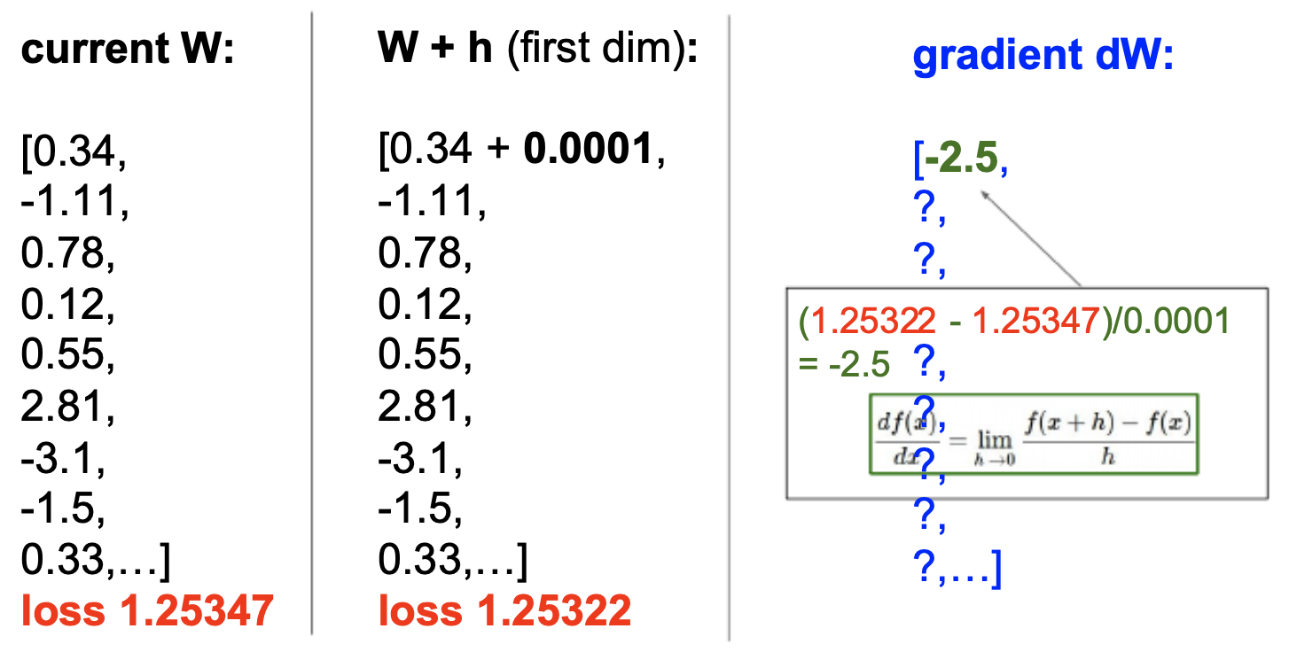
The following figure shows this process: by adding a small offset (\(h = 0.0001\)) to a parameter and recomputing the loss, we approximate the gradient.
-
This method provides accurate approximations but is computationally very slow, since it requires recomputing the loss for each parameter. In practice, it is mainly used for gradient checking (debugging whether backpropagation is implemented correctly).
-
Instead, modern training uses calculus-based derivations (backpropagation) to compute exact gradients efficiently.
Updating Weights
-
Once we have the gradient, we update the weights as:
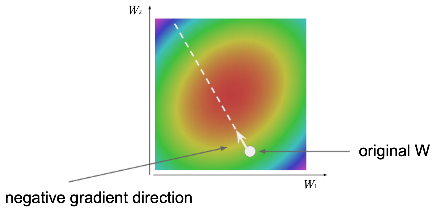
\[W := W - \alpha \nabla_W L\]- where \(\alpha\) is the learning rate. This step can be visualized as moving along the negative gradient direction in a contour plot of the loss function.
Valley Analogy Revisited
-
We can again picture optimization as standing somewhere in a valley of the loss landscape. Each update corresponds to taking a step downhill, guided by gradients.
-
The following figure illustrates the process of minimizing the loss function — gradient descent navigates the valley by repeatedly adjusting weights in the direction of steepest descent, with step size controlled by the learning rate \(\alpha\).
Challenges in Optimization
- Local minima and saddle points: Non-convex landscapes may contain many low regions. Saddle points (flat zones where gradients vanish) are often more problematic than true local minima.
- Vanishing/exploding gradients: In very deep networks, gradients may shrink toward zero or explode uncontrollably, disrupting training.
- High dimensionality: Modern models with millions of parameters require efficient algorithms and hardware acceleration.
Gradient Descent Variants
- Gradient Descent is the cornerstone of optimization in machine learning. While the basic idea — updating parameters in the opposite direction of the gradient — is simple, there are several practical ways to compute and apply gradients. These approaches trade off accuracy of gradient estimation against computational efficiency.
Batch Gradient Descent
- In Batch Gradient Descent, the gradient is computed using the entire training dataset of size \(N\):
- The update rule becomes:
-
Advantages:
- Provides the exact gradient of the loss over the dataset.
- Guarantees a stable and smooth path toward convergence.
-
Disadvantages:
- Extremely expensive for large datasets (millions of examples).
- Requires storing the entire dataset in memory, which is often impractical.
-
For this reason, pure batch gradient descent is rarely used in modern deep learning.
Stochastic Gradient Descent (SGD)
- Stochastic Gradient Descent improves computational efficiency by computing the gradient using only one randomly chosen training example:
- Update rule:
-
Advantages:
- Very fast updates — only one example is needed at a time.
- Introduces randomness, which helps escape saddle points and poor local minima.
-
Disadvantages:
- The gradient is a noisy approximation of the true gradient.
- The optimization path zig-zags heavily, which may slow convergence.
-
Despite its noisy updates, SGD has been incredibly influential because of its scalability to large datasets.
-
The figure below illustrates the calculation of partial derivatives to approximate the gradient. In practice, SGD computes gradients from only one or a few data points at a time, introducing randomness but keeping computations efficient.
Mini-Batch Gradient Descent
- Mini-Batch Gradient Descent is the most widely used compromise between batch and stochastic approaches. Instead of using the full dataset or just a single example, it uses a small batch of size \(M\):
- Update rule:
-
Advantages:
- Balances stability (less noisy than SGD) with efficiency (faster than full batch).
- Exploits hardware parallelism (GPUs and TPUs handle matrix operations on batches efficiently).
- Improves generalization by adding a mild amount of stochasticity.
-
Disadvantages:
- Still involves hyperparameter tuning for batch size and learning rate.
-
Typical mini-batch sizes range from 32 to 256, depending on memory capacity and the problem.
Comparing the Variants
- Batch GD: Precise but impractical for very large datasets.
- SGD: Very fast, noisy, but good for escaping bad regions.
-
Mini-Batch GD: The standard in deep learning — stable, efficient, and scalable.
- In modern practice, when people say “SGD,” they usually mean Mini-Batch SGD, often enhanced with advanced techniques such as momentum, adaptive learning rates, or gradient clipping.
The Optimization Loop
-
Training a neural network is an iterative process: parameters are repeatedly adjusted to minimize the loss. This cycle of forward passes, loss computation, backward passes, and parameter updates forms the backbone of all modern deep learning.
-
The loss tells us what to improve, while optimization decides how to improve it. Iterating this loop over many epochs gradually transforms raw parameters into a model that captures meaningful patterns in data.
The General Training Procedure
-
Initialize Parameters
- Start with random (or carefully designed) weights \(W\) and biases \(b\).
- Initialization matters: poor choices can lead to vanishing/exploding gradients or slow convergence.
-
Loop Over Epochs An epoch is one complete pass over the training dataset. Models typically train for many epochs.
- Shuffle Data: Randomizing prevents systematic bias in mini-batch composition.
-
Loop Over Mini-Batches: For each batch of size \(M\):
-
Forward Pass: Compute predictions
\[s = f(x; W, b)\] -
Loss Calculation:
\[L = \frac{1}{M} \sum_{i=1}^M L_i(f(x_i; W, b), y_i)\] - Backward Pass: Compute gradients via backpropagation.
-
Parameter Update: Adjust weights:
\[W_{\text{new}} = W - \eta \nabla_W L\]
-
-
Validation Step Evaluate periodically on held-out validation data:
- Monitors generalization.
- Enables early stopping before overfitting.
Key Considerations in the Loop
-
Learning Rate Scheduling A fixed \(\eta\) may be inefficient. Common schedules include exponential decay, cosine annealing, and step decay.
-
Number of Epochs Too few → underfitting; too many → overfitting. The optimal point is found via validation monitoring.
-
Regularization During Training Techniques like dropout, weight decay, and batch normalization are often integrated into the loop to boost generalization.
-
Checkpointing Saving weights at intervals prevents loss of progress and allows resuming training.
-
The optimization loop is thus the engine of learning: loss functions define the destination, gradients indicate direction, and the iterative loop provides the mechanism to get there.
Citation
If you found our work useful, please cite it as:
@article{Chadha2020LossFunctions,
  title   = {Loss Functions},
  author  = {Chadha, Aman},
  journal = {Distilled Notes for Stanford CS231n: Convolutional Neural Networks for Visual Recognition},
  year    = {2020},
  note    = {\url{https://aman.ai}}
}