CS231n • Introduction to Computer Vision
- Overview
- Why is Computer Vision Hard?
- Image Features
- The Rise of Neural Networks
- A Data-driven Approach
- The Computer Vision Pipeline
- Citation
Overview
-
Computer vision, at its core, is a field that aims to teach computers how to understand and interpret images. The fundamental goal is to replicate, and in many cases surpass, the human ability to perceive and analyze visual information. With the explosion of image data available today from sources like smartphones, drones, satellites, surveillance cameras, and autonomous vehicles, the development of algorithms to analyze this information has become crucial. For context, Cisco predicted that by 2022, video would account for approximately 82% of all internet traffic, and as of 2019, YouTube alone produced about 500 hours of new content every minute. Such scale makes it humanly impossible to monitor or annotate even a fraction of this data, highlighting the need for algorithms capable of perception at massive scale.
-
The field of computer vision is highly interdisciplinary. It draws from neuroscience (to understand biological vision systems), optics (to model imaging processes), robotics (to apply perception for decision-making and control), machine learning (to extract patterns and generalize), and graphics (to simulate and reconstruct).
-
At its core, computer vision sits at the intersection of mathematics, computer science, psychology, biology, physics, and engineering. Foundational works in vision such as Marr’s Vision: A Computational Investigation emphasized that perception should be studied as an information processing problem—a perspective that continues to influence modern approaches.
Vision in Evolution
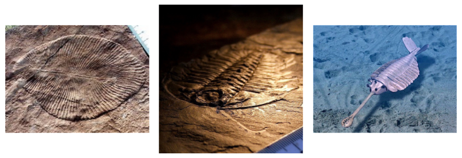
- To appreciate the profound importance of vision, one can look back to around 540 million years ago, during the Cambrian explosion, when the number of animal species on Earth dramatically increased from a few to hundreds of thousands over a short period of about 10 million years. This event is known as evolution’s “big bang”.
- Andrew Parker proposed in his book In the Blink of an Eye that this rapid evolutionary burst was catalyzed by the development of vision. Once animals could see, they gained powerful advantages: finding prey, avoiding predators, and navigating more complex environments. This forced other species to evolve rapidly, creating an evolutionary arms race.
- The following figure presents fossils of animals that existed around 540 million years ago.
From Biological Vision to Cameras
-
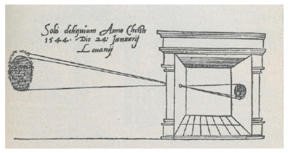
Around 2000 years ago, the early mechanisms of animal vision inspired devices that led to the invention of the camera. By the mid-1550s, the camera obscura became a pivotal tool in both art and science. It consisted of a darkened room or box with a small pinhole that projected an inverted image of the outside scene onto a surface inside. Artists like Johannes Vermeer are thought to have used this device to aid in their paintings. From this humble beginning, cameras evolved dramatically—first chemically (film photography) and later digitally (CCD and CMOS sensors). Today, cameras are so ubiquitous that it is estimated there are more cameras than humans on Earth, enabling the collection of visual data on an unprecedented scale.
-
The following figure presents work from 1544 on the creation of the pinhole image or camera obscura.
Neuroscience Foundations
-
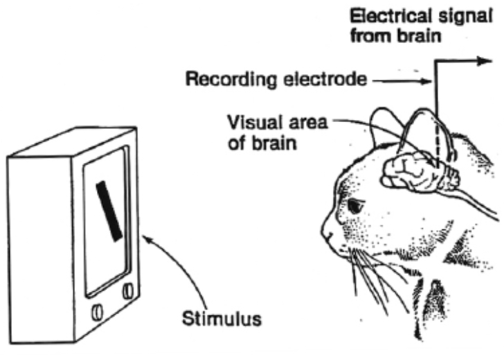
The scientific understanding of vision took a leap forward in the 20th century. In 1959, David Hubel and Torsten Wiesel conducted landmark experiments on cats’ visual cortices. By implanting microelectrodes, they observed that neurons in the visual cortex responded selectively to oriented edges and lines. This work, later earning them the Nobel Prize in Physiology or Medicine in 1981, revealed that biological vision operates in a hierarchical manner: early layers detect simple features (edges, orientations, motion), while higher layers combine these into more complex representations (shapes, textures, and eventually objects).
-
This principle directly inspired the architecture of modern artificial neural networks for vision, particularly convolutional neural networks (CNNs) (LeCun et al., 1989). The notion of hierarchically organized processing units in artificial systems can be traced back to this biological insight.
-
The following figure presents a photo of Hubel and Wiesel, who received the Nobel Prize in Physiology or Medicine in 1981 for their discoveries concerning information processing in the visual system.
Why is Computer Vision Hard?
-
Despite its long history, computer vision remains one of the most challenging problems in artificial intelligence. Unlike structured data such as text, where symbols (letters or words) have discrete boundaries and relatively consistent representations, images are continuous signals. They can vary widely in appearance due to countless environmental and contextual factors. This introduces a huge amount of variability in the input data, making it difficult for algorithms to generalize effectively.
-
A robust computer vision system must recognize an object regardless of its appearance, orientation, or background. The key challenge is building invariant representations—representations that are insensitive to irrelevant variations (lighting, scale, occlusion) but still capture the essential features of an object. Early frameworks, such as Marr’s theory of vision (Marr, 1982), conceptualized vision as a series of representational stages, from raw input to abstract 3D structures. This idea continues to guide modern deep learning systems.
Early Attempts: From Geometric Worlds to Real Images
-
The field of computer vision formally began in the early 1960s. One of the first doctoral theses in the area was by Larry Roberts (1963), who attempted to reconstruct and recognize primitive 3D shapes from simple 2D drawings (Roberts, 1963). Just a few years later, in 1966, MIT’s Artificial Intelligence Group ambitiously launched the Summer Vision Project, which proposed that a group of students could build a significant part of a visual system in a single summer (Minsky, 1966). The project underestimated the complexity of vision but spurred decades of research.
-
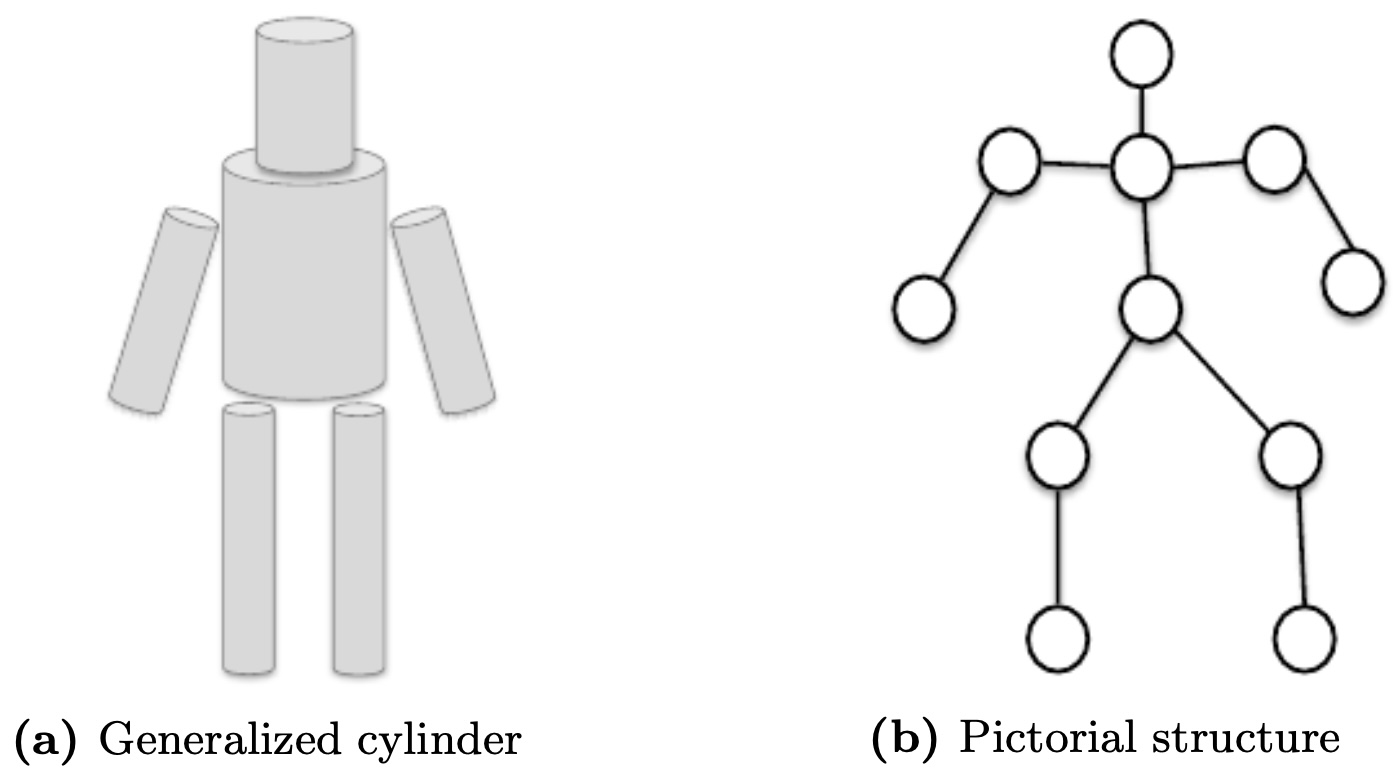
By the 1970s, researchers moved beyond toy environments of geometric primitives and began exploring ways to represent real-world objects. Among the most influential ideas were generalized cylinders and pictorial structures (Fischler & Elschlager, 1973), which decomposed objects into parts with geometric relations. These abstractions foreshadowed part-based models in the 2000s and deep networks today.
-
The following figure presents different ways of representing an object using generalized cylinders and pictorial structures.
Marr’s Framework
-
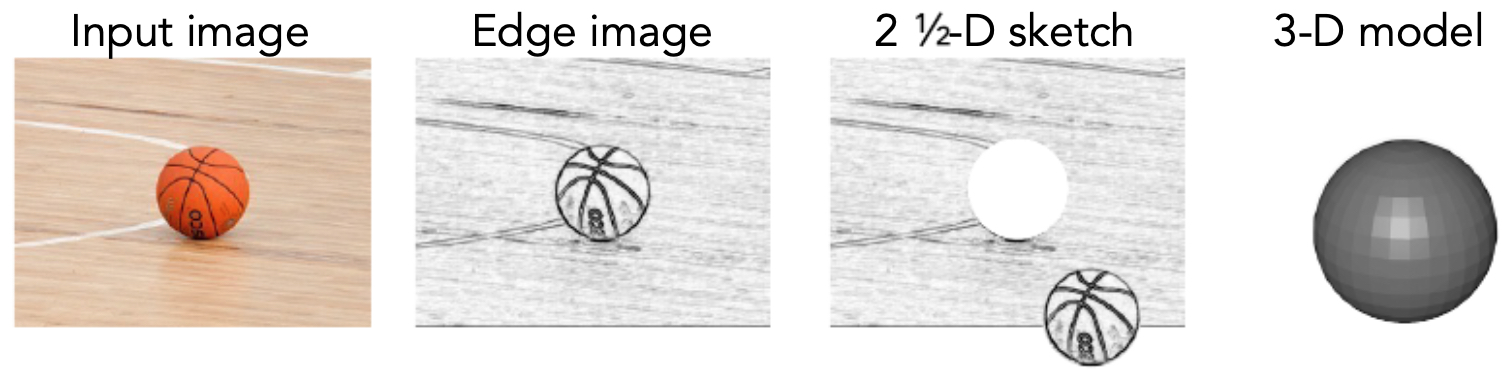
In 1982, David Marr’s influential book formalized a framework for visual perception. He described vision as a computational process of representations. Starting from an input image, the visual system extracts edges, curves, and other local structures to form a primal sketch. From there, depth cues are combined into what Marr called a 2.5D sketch, which encodes surfaces and their orientations relative to the viewer. Finally, these intermediate representations are assembled into a full 3D model that supports recognition and reasoning.
-
This hierarchical view closely matches both biological findings (Hubel & Wiesel) and modern artificial networks, where shallow layers capture edges, middle layers capture shapes, and deep layers build semantic categories.
-
The following figure presents the Marr framework, which describes the process of visual representation from raw image to 3D structure.
The Role of Segmentation
-
By the late 1990s, researchers realized that recognition could not succeed without solving segmentation—the problem of partitioning an image into meaningful regions. For example, a self-driving car must separate pedestrians, vehicles, roads, and signs from raw pixels. Segmentation provided a stepping stone from low-level features to higher-level understanding (Shi & Malik, 2000).
-
The following figure presents an example of image segmentation, with the original image on the left and its segmented counterpart on the right.

Sources of Variation
-
Even with segmentation, recognition faces immense variability. Below are the major sources that make vision hard:
- Viewpoint Variation: The same object looks drastically different from different perspectives. A car from the front shows headlights, while from the side it shows doors. Datasets such as Pascal VOC and MS COCO were designed to capture this diversity.
- Scale Variation: The size of objects changes with distance. Multi-scale methods like feature pyramids (Lin et al., 2017) address this.
- Illumination Variation: Lighting conditions profoundly affect appearance. Normalization and data augmentation attempt to overcome this.
- Deformation: Biological objects (e.g., people, cats) change shape constantly. Deformable part models (Felzenszwalb et al., 2010) were one early solution.
- Occlusion: Objects are often partially hidden (e.g., pedestrians behind cars). This remains a key challenge in safety-critical domains.
- Intra-class Variation: Members of the same category can look very different (e.g., Chihuahua vs. Great Dane). Large datasets like ImageNet capture this diversity.
- Background Clutter: Recognizing objects amid noisy or overlapping scenes is far harder than in clean backgrounds.
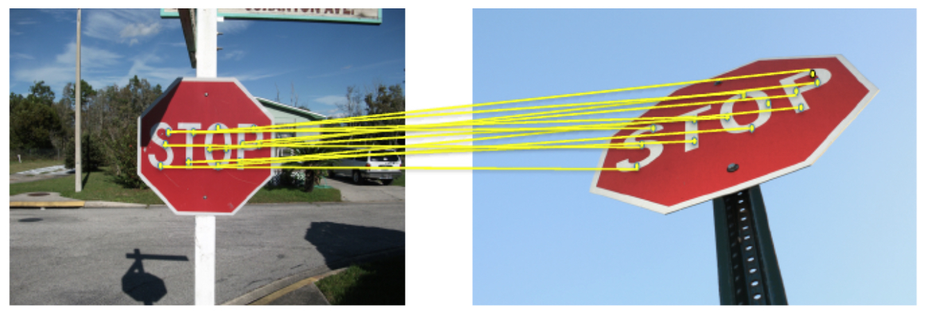
-
The following figure illustrates identifying features on two images of the same object with different variance, demonstrating the difficulty of building invariant representations.
Dataset Benchmarks
-
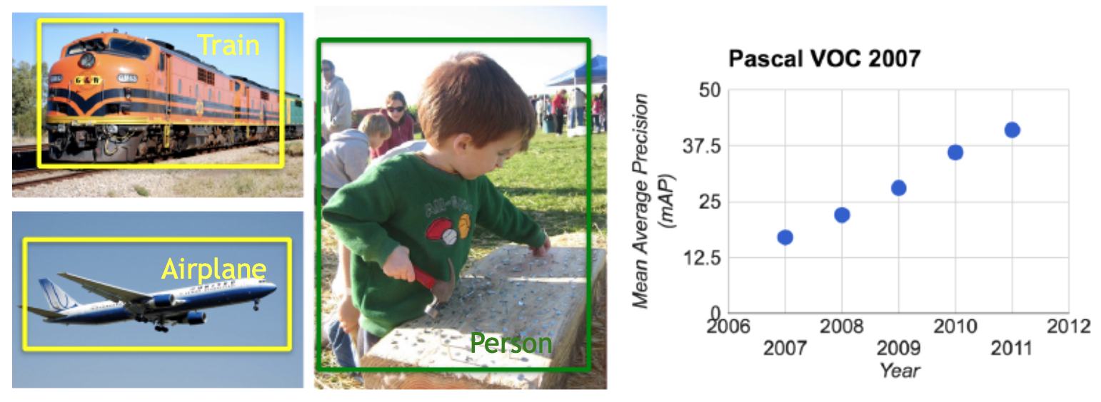
To measure progress and expose difficulties, benchmark datasets became essential. In the 2000s, the PASCAL Visual Object Classes Challenge (VOC) became a standard, covering 20 object categories with varied viewpoints, occlusions, and clutter. This benchmark revealed wide performance gaps between algorithms and human perception, motivating advances in feature extraction and learning methods.
-
The following figure shows examples from the PASCAL dataset (left) and the performance trajectory of algorithms on this benchmark (right).
Limitations of Current Systems
- Even state-of-the-art systems remain brittle. A striking demonstration comes from adversarial examples (Szegedy et al., 2013): tiny, imperceptible changes to pixel patterns can completely flip a model’s prediction. This fragility underscores that, despite tremendous progress, computer vision is far from solved. The inherent variability, ambiguity, and complexity of visual input ensure that perception remains one of the hardest challenges in AI.
Image Features
-
Before the deep learning revolution, computer vision systems relied heavily on handcrafted features rather than learning directly from raw pixel data. The central idea was to transform raw pixel intensities into more structured and meaningful representations that a classifier (such as an SVM or logistic regression) could use effectively.
-
These methods dominated the 1990s and 2000s, shaping applications like face detection, object recognition, and image retrieval. Among the most influential were:
- Color Histograms (Swain & Ballard, 1991) – summarized distributions of colors in an image.
- HOG (Histogram of Oriented Gradients) (Dalal & Triggs, 2005) – encoded edge orientations for robust object detection.
- SIFT (Scale-Invariant Feature Transform) (Lowe, 2004) – detected keypoints and descriptors invariant to scale and rotation.
- Bag of Visual Words (BoW) (Csurka et al., 2004) – aggregated local descriptors into histograms for classification.
-
One of the landmark algorithms from this era was the Viola–Jones face detector (2001) (Viola & Jones, 2001). Using a boosting framework over Haar-like features, it enabled real-time face detection on consumer hardware—so successful that it was quickly integrated into digital cameras. Around the same time, David Lowe’s SIFT algorithm transformed recognition by allowing robust matching of local features between images, enabling applications such as object recognition, panorama stitching, and 3D reconstruction.
-
While handcrafted features were powerful, they required enormous domain expertise and were often task-specific. A feature that worked well for face detection might fail completely for recognizing vehicles or animals. This “engineering bottleneck” motivated the eventual shift to data-driven deep learning approaches.
Why Extract Features?
-
Raw images are simply grids of pixel values. For instance, a grayscale image of size \(100 \times 100\) contains 10,000 intensity values, while an RGB image triples this number. These values alone are not very informative for a linear classifier, since small changes in lighting, rotation, or viewpoint could drastically alter pixel values while the semantic meaning (e.g., a cat) remains the same.
-
Image features aimed to solve this by capturing invariant properties of images:
- Edges and contours that describe shapes.
- Color distributions that capture the overall appearance.
- Texture patterns that characterize surfaces (e.g., fur, grass).
-
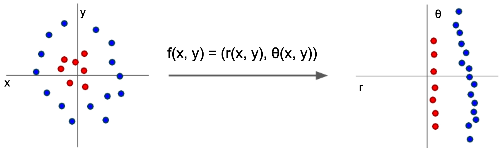
The figure illustrates how feature extraction transforms raw data into a feature space where classification becomes easier. On the left, raw pixel intensities may not be linearly separable. On the right, with meaningful features, a simple linear classifier can separate the classes effectively.
Examples of Handcrafted Features
-
Color Histograms Capture the distribution of colors across an image. They ignore spatial arrangement but provide a robust summary of appearance.
-
Histogram of Oriented Gradients (HOG) Encode edges and gradient directions, useful for recognizing shapes and outlines (e.g., pedestrians, animals).
-
Bag of Visual Words (BoW) Treats local features as “visual words” and builds a histogram representation, analogous to how text documents are modeled in natural language processing.
Strengths of Handcrafted Features
- Computationally efficient to calculate.
- Often invariant to basic transformations like scaling, translation, or rotation.
- Effective for traditional machine learning classifiers.
Limitations
- Task-specific: Features had to be carefully designed for each application. A feature that works well for face detection might fail for vehicle recognition.
- Limited expressiveness: Handcrafted features cannot easily capture higher-level semantic concepts (e.g., “this is a cat sitting on a chair”).
- Engineering burden: Designing, tuning, and combining features required significant human expertise.
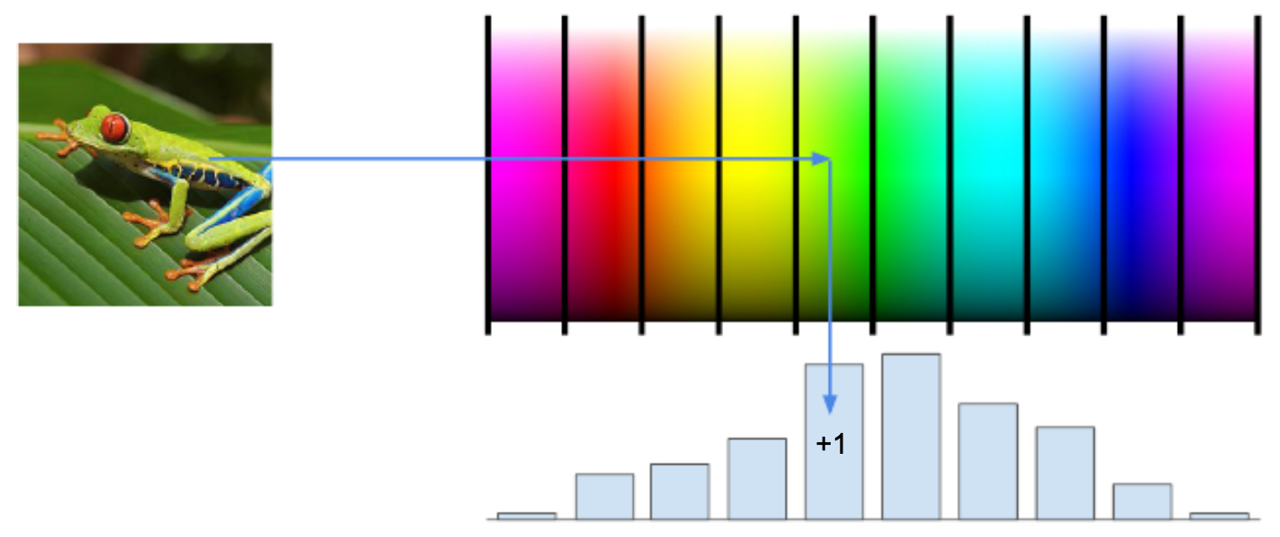
Color Histogram
- A Color Histogram is one of the simplest yet most widely used feature descriptors in early computer vision. It captures the distribution of colors in an image, essentially summarizing which colors are present and in what proportion. Importantly, it disregards the spatial arrangement of colors — only their frequency matters.
- While limited in expressive power, color histograms represented an important step in bridging raw pixel data and useful visual features. They are often combined with other descriptors (like texture or edges) to form richer representations.
How It Works
-
Define Color Bins
- The color range (e.g., 0–255 for each RGB channel) is divided into discrete bins.
- For instance, splitting each channel into 16 bins results in a total of \(16 \times 3 = 48\) features.
-
Count Pixels
- For each pixel in the image, determine which bin its value falls into.
- Increment the count for that bin.
-
Normalize
- Normalize the histogram so that it becomes invariant to image size.
- This ensures a small thumbnail and a large high-resolution version of the same image yield comparable histograms.
- The figure illustrates feature extraction using color histograms. Each pixel contributes to bins corresponding to Red, Green, and Blue intensities. The final histogram encodes the overall color distribution of the image.
Strengths
- Simplicity: Very fast to compute and easy to implement.
- Invariant to rotation and scaling: Since only color counts are considered, transformations like rotation do not change the histogram.
- Effective for coarse tasks: Works well in distinguishing broad categories like “day vs. night,” “indoor vs. outdoor,” or identifying objects with distinctive color schemes (e.g., sky, vegetation, road).
Weaknesses
- No spatial information: A picture of a blue sky and a blue car on a road could have similar color histograms, even though the content is very different.
- Sensitive to illumination: Lighting changes can shift color distributions, making histograms less reliable under varied conditions.
- Limited discriminative power: Different objects with similar color palettes (e.g., a red apple and a red car) may be indistinguishable using histograms alone.
Use Cases
- Image retrieval: Searching databases for images with similar color distributions.
- Scene classification: Differentiating between categories like “forest,” “desert,” or “ocean.”
- Tracking in videos: Tracking a colored object (e.g., a red ball) by maintaining its histogram across frames.
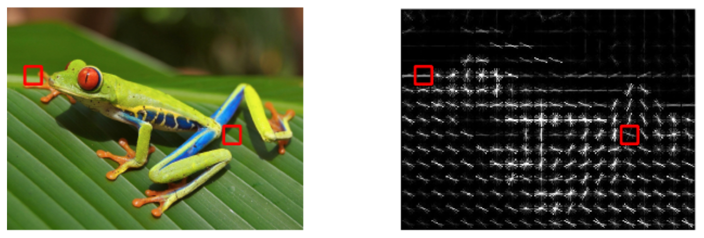
Histogram of Oriented Gradients (HOG)
- The Histogram of Oriented Gradients (HOG) is a more sophisticated feature descriptor than color histograms, designed to capture the shape and structure of objects within an image. Instead of focusing on colors, HOG encodes the distribution of edge directions and gradient intensities. This makes it especially effective for object detection, since the outline and silhouette of objects are often more discriminative than their color.
- HOG represented a significant leap forward in feature engineering. By focusing on local edge structures, it provided classifiers with rich information about object geometry. However, like color histograms, HOG has largely been replaced by features automatically learned by deep convolutional networks — which can capture not only edges but also progressively higher-level concepts.
How It Works
-
Divide the Image into Cells
- The image is split into small regions, typically \(8 \times 8\) or \(16 \times 16\) pixels.
- Each cell will produce its own local histogram of gradient directions.
-
Compute Gradients
-
For every pixel in a cell, compute the horizontal and vertical gradients: \(G_x = I(x+1, y) - I(x-1, y)\) \(G_y = I(x, y+1) - I(x, y-1)\)
-
From these, calculate gradient magnitude and orientation: \(\text{magnitude} = \sqrt{G_x^2 + G_y^2}, \quad \text{orientation} = \arctan\left(\frac{G_y}{G_x}\right)\)
-
-
Bin the Orientations
- Divide orientations into bins (e.g., 9 bins for \(0^\circ\)–\(180^\circ\)).
- Each pixel votes for a bin based on its gradient orientation, weighted by its gradient magnitude.
-
Normalize Blocks
- To reduce the effect of illumination or contrast changes, group neighboring cells into larger blocks (e.g., \(2 \times 2\) cells).
- Normalize the histograms within each block.
-
Concatenate Histograms
- Finally, concatenate histograms from all blocks into a long feature vector that represents the entire image.
- The figure illustrates how gradient orientations are extracted and binned into histograms. Unlike color histograms, which focus on pixel intensity distributions, HOG emphasizes local edge patterns that describe object shapes.
Strengths
- Captures shape information: By encoding edges and gradients, HOG provides a strong description of object outlines and silhouettes.
- Illumination robustness: Normalization makes the feature less sensitive to changes in lighting or contrast.
- Proven effectiveness: HOG was famously used in the Dalal–Triggs pedestrian detector (2005), which set a new benchmark for detecting people in images.
Weaknesses
- Scale sensitivity: Objects of different sizes may produce different HOG representations unless scale-invariant techniques are added.
- Computational cost: More expensive to compute than simple color histograms, especially for high-resolution images.
- No semantic understanding: Like other handcrafted features, HOG captures low-level patterns but not higher-level concepts.
Use Cases
- Pedestrian detection: One of the most famous applications of HOG, enabling robust detection of people in surveillance and driving scenes.
- Object detection in general: Applied to vehicles, animals, and other structured objects where shape matters more than color.
- Texture recognition: Useful in differentiating surfaces with distinct edge distributions (e.g., bricks vs. grass).
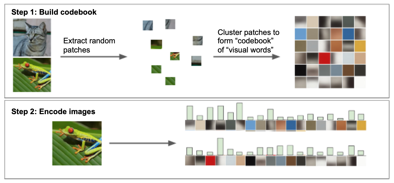
Bag of Words for Visual Recognition
- The Bag of Words (BoW) model is an approach that draws inspiration from natural language processing. In text analysis, a document can be represented as a histogram of word frequencies, disregarding the order of words but retaining their presence and relative importance. Similarly, in computer vision, the BoW model represents an image as a histogram of “visual words,” constructed from local feature descriptors.
- This method was a major advance before deep learning, as it allowed large image collections to be represented and compared efficiently.
- Although highly influential, BoW ultimately reached a performance ceiling due to its loss of spatial structure. Deep learning later surpassed it by automatically learning hierarchical features that preserved both local and global context. Nevertheless, BoW remains an important historical step in computer vision and is still used in some lightweight or resource-constrained applications.
The Process
-
Feature Extraction
- Local features (e.g., corners, edges, or distinctive patches) are extracted from each image.
- Common algorithms include SIFT (Scale-Invariant Feature Transform) and SURF (Speeded-Up Robust Features), which generate descriptors for image keypoints.
-
Visual Vocabulary Construction
- Combine local descriptors from many training images.
- Use clustering algorithms (commonly K-means) to group descriptors into clusters.
- Each cluster center becomes a visual word in the vocabulary.
- The vocabulary size \(K\) (typically hundreds or thousands) is a hyperparameter that controls granularity.
-
Mapping Features to Words
- For a new image, each extracted local descriptor is matched to the nearest cluster center (visual word).
- This step “quantizes” continuous descriptors into discrete categories.
-
Histogram Creation
- Count the occurrences of each visual word in the image.
- This count histogram becomes the image’s BoW feature vector.
- The figure illustrates the Bag of Words pipeline. Local features are clustered into a “visual vocabulary,” and each image is then represented as a histogram of visual word occurrences. This transforms raw local descriptors into a fixed-length vector suitable for classifiers.
Strengths
- Fixed-length representation: Regardless of image size or number of features, each image is represented as a \(K\)-dimensional vector.
- Translation and rotation invariance: Since spatial arrangement is ignored, shifting or rotating objects does not significantly change the histogram.
- Scalability: Enables efficient indexing and retrieval of large image databases.
Weaknesses
- Loss of spatial information: The arrangement of features is discarded. For example, the histogram cannot distinguish between a face (eyes above nose above mouth) and a scrambled arrangement of the same parts.
- Choice of vocabulary size: Too few clusters = overly coarse representation; too many clusters = overfitting and computational inefficiency.
- Dependence on feature extractors: The quality of BoW representations relies heavily on the robustness of the underlying local descriptors (e.g., SIFT).
Use Cases
- Image classification: BoW histograms can be fed into classifiers like SVMs for object recognition.
- Image retrieval systems: Efficiently matching histograms enables searching for visually similar images in large datasets.
- Scene recognition: Used for distinguishing categories like “beach,” “forest,” or “city” where global arrangements are less important than recurring local patterns.
The Rise of Neural Networks
-
For much of its history, computer vision relied on hand-engineered features. Researchers manually designed descriptors intended to capture important structures in an image—edges, corners, textures, or shapes—that would remain stable under changes in scale, rotation, or lighting. While powerful in controlled domains (e.g., face detection, document analysis), these handcrafted approaches faced two major limitations:
- Lack of generalization — features that worked for one task often failed in different settings.
- Human intuition bottleneck — progress depended on clever feature design rather than learning from data.
-
This paradigm shifted dramatically with the rise of neural networks, particularly convolutional neural networks (CNNs).
Why CNNs Were Revolutionary
-
Unlike handcrafted approaches, CNNs learn features automatically from raw data. Instead of defining what features to look for, researchers define an architecture, and the model learns to discover the most useful features during training.
-
Several factors catalyzed this breakthrough around the early 2010s:
- Massive labeled datasets such as ImageNet (Deng et al., 2009) with millions of images across thousands of categories.
- Increased computational power, especially GPUs, which allowed training deep networks at scale.
- Better optimization techniques, such as stochastic gradient descent with momentum and dropout regularization.
-
At the computational level, an image is simply a tensor (multi-dimensional array) of pixel values. For example, a 32 × 32 pixel RGB image is represented as:
\[32 \times 32 \times 3\]- where the last dimension corresponds to the color channels (Red, Green, Blue). Each entry is an intensity value (0–255). To a human, this is a cat or a car; to a computer, it is just numbers. The challenge is mapping this grid of values to semantic meaning.
Hierarchical Feature Learning
-
CNNs mirror the hierarchical organization of biological vision, first revealed by Hubel and Wiesel’s experiments on cats (Hubel & Wiesel, 1959):
- Early layers learn simple, low-level features (edges, corners, color gradients).
- Intermediate layers combine these into textures, contours, and object parts.
- Deeper layers capture abstract concepts like “cat face” or “car wheel.”
-
This hierarchy allows CNNs to progressively transform pixel values into semantic concepts.
From Pixels to Concepts
-
The goal of a CNN in classification tasks is to transform raw image tensors into class scores. The final layer often uses the softmax function to convert scores into probabilities:
\[p_j = \frac{e^{s_j}}{\sum_k e^{s_k}}\]- where \(s_j\) is the score for class \(j\), and \(p_j\) is its predicted probability. Networks are trained to maximize the probability of the correct label via loss functions such as cross-entropy.
The Breakthrough: AlexNet
-
The transformative moment came in 2012 with AlexNet (Krizhevsky et al., 2012). Submitted to the ImageNet Large Scale Visual Recognition Challenge (ILSVRC), AlexNet reduced classification error rates by nearly half compared to the best handcrafted systems. Its innovations included:
- Deep architecture (8 layers, unprecedented at the time).
- GPU acceleration for large-scale training.
- ReLU activations for faster convergence.
- Dropout regularization to combat overfitting.
-
This single model marked the beginning of the deep learning revolution in computer vision.
-
The following figure presents the evolution of ImageNet top-5 error rates year after year, highlighting the dramatic performance leap achieved by AlexNet in 2012 and the rapid improvements that followed.
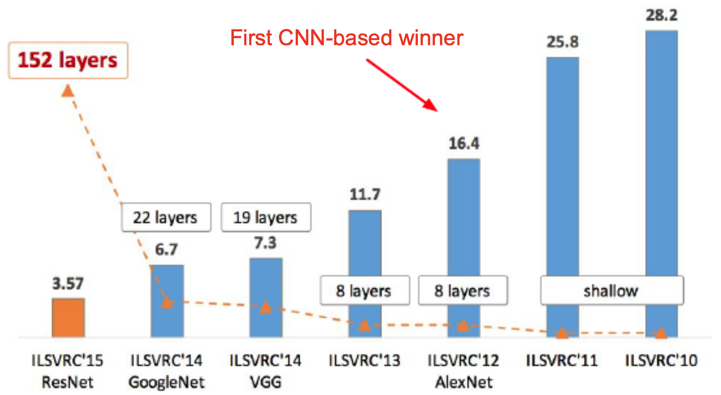
Beyond AlexNet
-
After AlexNet, progress accelerated rapidly:
- VGG (Simonyan & Zisserman, 2014) showed that simply increasing network depth (up to 19 layers) could improve accuracy.
- ResNet (He et al., 2015) introduced residual connections, enabling the training of extremely deep models (100+ layers).
- Vision Transformers (ViTs) (Dosovitskiy et al., 2020) departed from convolution entirely, using self-attention to capture long-range dependencies across an image.
-
These advances pushed performance beyond human accuracy on benchmark recognition tasks, while also opening new frontiers in detection, segmentation, and generative modeling.
A Data-driven Approach
-
The modern paradigm in computer vision is data-driven. Instead of handcrafting features or rules, researchers now rely on learning from vast datasets. This shift became especially clear in the 2000s: small datasets with a few thousand examples often led to overfitting, where models performed well in training but failed on unseen data (Torralba & Efros, 2011). To address this, researchers created large-scale datasets capable of capturing the diversity and variance present in real-world images.
-
The most influential was ImageNet (Deng et al., 2009), which contained over 14 million labeled images across 22,000 categories. The associated ImageNet Large Scale Visual Recognition Challenge (ILSVRC), introduced in 2010, required algorithms to classify among 1,000 categories, measuring success by whether the correct label appeared in the top-5 predictions. This benchmark created a global competition that drove rapid progress and culminated in the breakthrough of AlexNet (2012).
-
Other benchmarks also shaped the field:
- COCO (Common Objects in Context) (Lin et al., 2014) – focused on object detection, segmentation, and captioning.
- PASCAL VOC (Everingham et al., 2010) – provided a standardized testbed for recognition with varied viewpoints and occlusions.
- Open Images (Kuznetsova et al., 2020) – extended large-scale labeling to detection and segmentation tasks.
The Role of Data
- Data is the lifeblood of modern vision systems. The more diverse and extensive the dataset, the better a trained model can generalize to unseen conditions. However, models are only as good as their training distributions. For example, a network trained on daylight driving images often fails at nighttime or in rain. This makes dataset diversity and domain adaptation central concerns in modern research.
Scoring Functions and Hypothesis Spaces
-
At the core of any learning system is a scoring function (or hypothesis class).
-
In traditional machine learning, this might be a linear classifier:
\[s = w^T x + b\]- where \(x\) is the feature vector, and \(w\) and \(b\) are learned parameters.
-
In deep learning, the scoring function is parameterized by millions (or billions) of weights distributed across multiple layers. This massive hypothesis space allows CNNs, ResNets, and Transformers to model highly complex, nonlinear relationships between pixels and semantic labels.
Loss Functions and Learning Objectives
-
Learning requires a way to measure how well a model’s predictions match reality. This is the role of the loss function.
-
For classification, the most widely used is cross-entropy loss:
\[L = -\sum_j y_j \log p_j\]- where \(y_j\) is the ground-truth label (one-hot encoded), and \(p_j\) is the predicted probability for class \(j\).
-
For other tasks, alternative losses apply:
- Smooth L1 Loss for bounding-box regression in detection.
- Dice Loss / IoU Loss for segmentation masks.
- Adversarial Loss for generative adversarial networks (GANs) (Goodfellow et al., 2014).
-
The choice of loss function fundamentally shapes model behavior.
Why This Paradigm Works
-
This triad — large datasets, expressive scoring functions, and well-designed loss functions — defines supervised learning in computer vision. Their interaction explains the dramatic progress of the past decade:
- Bigger datasets → better generalization.
- More powerful scoring functions → ability to capture complex relationships.
- Appropriate loss functions → meaningful and stable training.
-
This paradigm scales naturally: as data availability grows and compute accelerates, models continue to improve in accuracy, robustness, and versatility. The trajectory of progress has shown that, given enough data and the right architectures, models can often exceed human performance on benchmark recognition tasks.
The Computer Vision Pipeline
-
Training a computer vision model can be thought of as a pipeline, where raw sensory input (images) is gradually transformed into useful outputs (labels, detections, or segmentations). This pipeline embodies the data-driven methodology described earlier, integrating representation learning, optimization, and inference into a unified framework.
-
While details vary by task (classification, detection, segmentation, generation), the underlying loop remains consistent:
input → representation → classification → optimization → inference → deployment
-
This framework evolved from early handcrafted approaches, through segmentation-based methods in the 1990s, to today’s large-scale deep networks.
Step 1: Input
-
The pipeline begins with raw image data, represented as a tensor of pixel intensities:
\[I \in \mathbb{R}^{H \times W \times C}\]- where \(H\) is the image height, \(W\) the width, and \(C\) the number of color channels (typically 3 for RGB).
-
Before feeding images into a model, preprocessing is crucial. Common operations include:
- Resizing (e.g., scaling all images to 224 × 224 for ImageNet-trained CNNs).
- Normalization (subtracting dataset mean, dividing by standard deviation).
- Data augmentation: random crops, horizontal flips, color jittering, Gaussian noise, etc.
-
Augmentations, first popularized in AlexNet (Krizhevsky et al., 2012), simulate real-world variability, making models more robust to changes in viewpoint, lighting, and occlusion.
Step 2: Feature Extraction
-
Once images are input, the next stage is feature extraction. In classical vision, feature extraction relied on hand-engineered descriptors:
- Edges (Canny, Sobel filters).
- Local features (SIFT, SURF).
-
Part-based models (generalized cylinders, pictorial structures).
-
Automatic feature engineering is the heart of modern neural networks, which learn hierarchical representations:
- Early layers capture low-level features: edges, corners, textures.
- Intermediate layers capture mid-level features: contours, parts, shapes.
- Deeper layers capture high-level semantics: objects, categories, scene context.
-
This hierarchical representation allows the network to build invariance (ignoring irrelevant changes, such as lighting) while retaining discriminative power (preserving object identity).
-
For example:
- ResNet (He et al., 2015) showed that deeper hierarchies, when stabilized with residual connections, dramatically improve performance.
- Vision Transformers (ViTs) (Dosovitskiy et al., 2020) replaced convolution with self-attention, allowing direct modeling of long-range dependencies in images.
- This stage is analogous to biological vision, where neurons in early visual cortex detect oriented edges (Hubel & Wiesel, 1959).
Step 3: Classification, Detection, Recognition, etc.
- Classification:
-
The extracted feature representation is fed into a classifier, which maps features to category scores.
-
In simple terms:
\[s_j = w_j^T f(x) + b_j\]- where \(f(x)\) is the learned feature vector, \(w_j\) and \(b_j\) are classifier parameters, and \(s_j\) is the score for class \(j\).
-
To convert these scores into probabilities, we use the softmax function:
- The predicted probability distribution is then compared against the true label using a loss function such as cross-entropy. This step ensures the model learns to maximize the probability of the correct class.
-
-
Detection and Recognition: Beyond classification, vision often requires localizing and identifying objects. Early breakthroughs included:
- Viola–Jones face detector (2001) (Viola & Jones), which used Haar-like features and boosting to enable real-time face detection.
- SIFT (1999–2004) (Lowe), which enabled matching features across images despite scale or rotation differences.
Modern approaches extend this to general object detection:
- Faster R-CNN (Ren et al., 2015).
- YOLO (Redmon et al., 2016).
These architectures integrate detection directly into the pipeline.
Step 4: Optimization and Learning Loop
-
Training is iterative. The core loop is:
- Forward pass: Compute predictions.
- Loss calculation: Compare predictions to ground truth.
- Backpropagation: Compute gradients of loss w.r.t. parameters.
- Parameter update: Adjust parameters via an optimizer (SGD, Adam, etc.).
-
Formally, parameters \(\theta\) are updated as:
\[\theta \leftarrow \theta - \eta \nabla_\theta L(\theta)\]- where \(\eta\) is the learning rate, and \(L\) the loss function.
-
Repeated over many epochs, this loop gradually refines the model.
Step 5: Inference
-
Once trained, the model is deployed for inference on unseen data. The same pipeline applies, but without gradient updates—only forward passes are performed.
-
Depending on the architecture, inference can serve multiple tasks:
- Classification (e.g., ResNet on ImageNet).
- Object detection (e.g., Faster R-CNN (Ren et al., 2015), YOLO (Redmon et al., 2016)).
- Semantic segmentation (e.g., U-Net (Ronneberger et al., 2015)).
- Image generation/reconstruction (e.g., GANs (Goodfellow et al., 2014), diffusion models (Ho et al., 2020)).
Step 6: Deployment and Feedback
-
In real-world applications (autonomous driving, medical imaging, industrial inspection), deployment is not the end. Models must be continuously monitored for performance degradation.
- Distribution shift (data differing from training distribution) can cause failures.
- Feedback loops (collecting new data from deployment environments) enable retraining and domain adaptation.
-
Active learning and continual learning approaches help models remain robust in changing environments.
- This cyclical pipeline—training, deployment, monitoring, retraining—ensures that vision systems remain effective in dynamic, unpredictable real-world conditions.
Citation
If you found our work useful, please cite it as:
@article{Chadha2020IntroductionToComputerVision,
  title   = {Introduction to Computer Vision},
  author  = {Chadha, Aman},
  journal = {Distilled Notes for Stanford CS231n: Convolutional Neural Networks for Visual Recognition},
  year    = {2020},
  note    = {\url{https://aman.ai}}
}