CS231n • Image Classification
- Overview
- K-nearest neighbors
- Linear classifiers
- Neural Networks
- Convolutional Neural Networks (CNNs)
- Vision Transformers (ViTs)
- Modern Trends in Vision
- Citation
Overview
-
Image classification is a foundational task in computer vision where the goal is to assign a single label to an image from a predefined set of categories. At its core, the problem is deceptively simple: given an image, determine what object or scene it contains. For example, given a photo of a cat, the desired output is the label “cat”. Despite this apparent simplicity, the task is challenging because computers and humans perceive images in fundamentally different ways.
-
Most digital images are represented using pixels, which can be thought of as the smallest indivisible units of an image. Each pixel encodes three values corresponding to the intensities of red, green, and blue (RGB) channels. By combining these three channels, we can approximate the full spectrum of colors visible to the human eye. Thus, an image can be represented as a 3D tensor of numbers: height × width × 3 color channels. For example, a \(32 \times 32\) RGB image is represented as a tensor of shape (32, 32, 3). When flattened, this becomes a long vector, but flattening erases much of the spatial information that makes vision intuitive to humans.
-
The following figure shows how images are represented as a matrix of pixels when stored on a computer:
![]()
- While this tensor representation is mathematically convenient, it creates what is known as the semantic gap: humans perceive meaning (objects, scenes, relationships), but the computer only sees arrays of numbers. Bridging this gap is the central difficulty in image classification and related vision problems (Marr, 1982).
Challenges in Image Classification
-
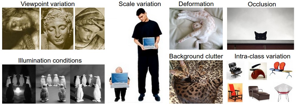
Unlike controlled laboratory conditions, real-world images vary drastically. Even images of the same object category can differ due to numerous factors:
- Viewpoint variation: An object looks different when seen from different angles.
- Scale variation: The size of the object changes depending on how far it is from the camera.
- Deformation: Some objects, like humans or animals, can bend or change shape.
- Occlusion: Objects may be partially hidden by other objects.
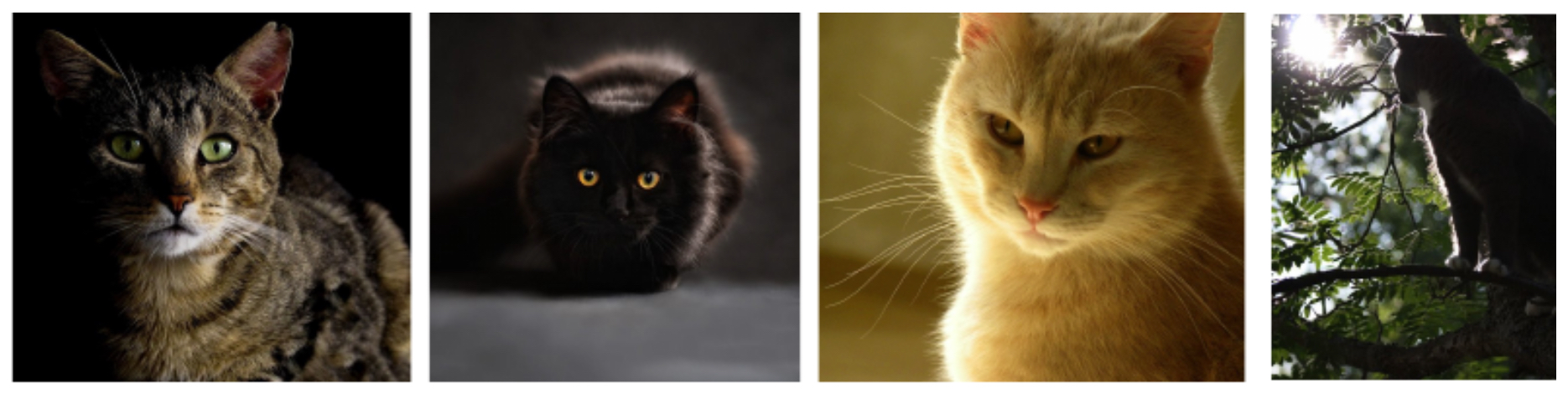
- Illumination changes: Lighting conditions alter pixel values dramatically.
- Background clutter: Objects often appear against distracting or noisy backgrounds.
- Intra-class variation: Different instances of the same category can look very different (e.g., different breeds of dogs).
-
The following figure visualizes these challenges, which make classification a non-trivial problem:
- For example, illumination alone can alter the intensity distribution of an image enough to make a simple algorithm fail. A white cat in dim lighting may appear visually closer to a gray dog under bright light. The following figure illustrates how lighting variation changes the pixel values of the same object:
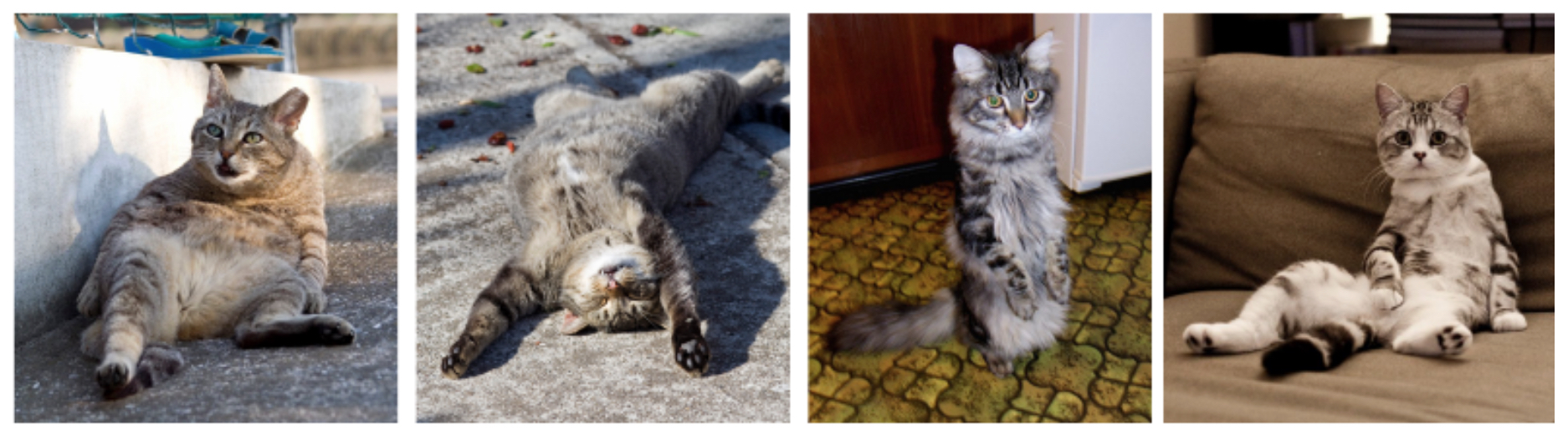
- Similarly, objects can take on multiple formations. For example, a human sitting, standing, or lying down should all be classified as “human”. The following figure demonstrates this challenge:
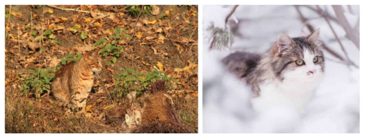
- Even when the object itself remains the same, background variation adds complexity. A single class, such as “car”, might appear on a highway, in a garage, or parked in a crowded city street. The following figure illustrates this challenge:
Early Attempts at Image Classification
-
Hard-coding the image classification problem with if-then rules turned out to be extremely difficult. Early methods relied on extracting hand-crafted features, such as edges and corners, using tools like the Canny edge detector or Harris corner detector (Lowe, 2004). The hope was that by detecting edges and corners, one could uniquely identify objects based on geometry, scale, or arrangement. However, this approach suffered from severe limitations because of real-world variability—objects in different lighting, poses, or backgrounds often share edges and corners with irrelevant regions.
-
The following figure shows an example of these early hard-coded attempts, where edges and corners were extracted in the hope of defining image categories:
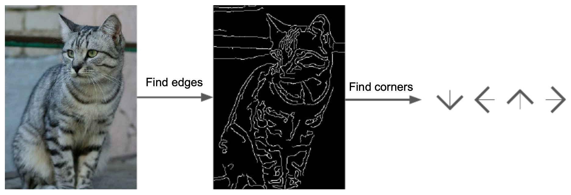
- These methods proved brittle and did not generalize well. They also required defining a set of features for each possible class label, which is infeasible given the vast variability of the visual world. This brittleness motivated the shift toward supervised learning approaches, where a dataset of labeled images is used to train a classifier. In supervised learning, the model learns mappings between pixel values and labels from data, allowing it to generalize to new unseen examples. This idea laid the foundation for the machine learning approaches that dominate computer vision today.
K-nearest neighbors
-
A key shift from early rule-based methods to modern computer vision was the adoption of data-driven algorithms. Instead of encoding rigid rules, researchers began to ask: what if we simply let the data define the rules? One of the earliest approaches in this paradigm was the nearest neighbor classifier (Cover & Hart, 1967).
-
The nearest neighbor algorithm works as follows: given a new image, we compare it to every image in the training set. The class label of the most similar training image is assigned to the test image. However, this naive version suffers greatly from the variance problem: two images of the same category can look very different due to changes in illumination, pose, background, and occlusion.
-
To mitigate this, researchers developed the K-nearest neighbors (KNN) algorithm. Instead of relying on just one closest example, KNN considers the K nearest training samples and assigns the majority label among them. This makes the model more robust to outliers and noise.
Computational complexity
-
The nearest neighbor approach has an unusual computational profile. Training consists of simply storing all training images, which is extremely fast (complexity of order O(1)). However, prediction requires comparing a test image to every training image, yielding runtime complexity of O(n), where n is the number of training samples. This is the opposite of what we typically want in practice: fast inference is more important than fast training, since deployed models must classify many test inputs efficiently.
-
Modern models like convolutional neural networks (CNNs) invert this tradeoff: they require long training times but produce extremely fast predictions at test time (LeCun et al., 1998).
Components of KNN
-
To implement KNN for image classification, two key components are required:
- A distance metric to measure similarity between images.
- A search algorithm to efficiently find the nearest neighbors.
-
The most common similarity measure is the Euclidean distance (the L2 norm). For two images \(I_1\) and \(I_2\), each represented as vectors of pixel intensities:
\[D(I_1, I_2) = \sqrt{\sum_{p} (I_1^p - I_2^p)^2}\]- where \(p\) indexes pixels. Conceptually, this computes the straight-line distance in high-dimensional space.
-
Another option is the Manhattan distance (the L1 norm):
- More generally, any Lp norm can be used:
-
The choice of metric significantly impacts classifier performance (Weinberger & Saul, 2009).
-
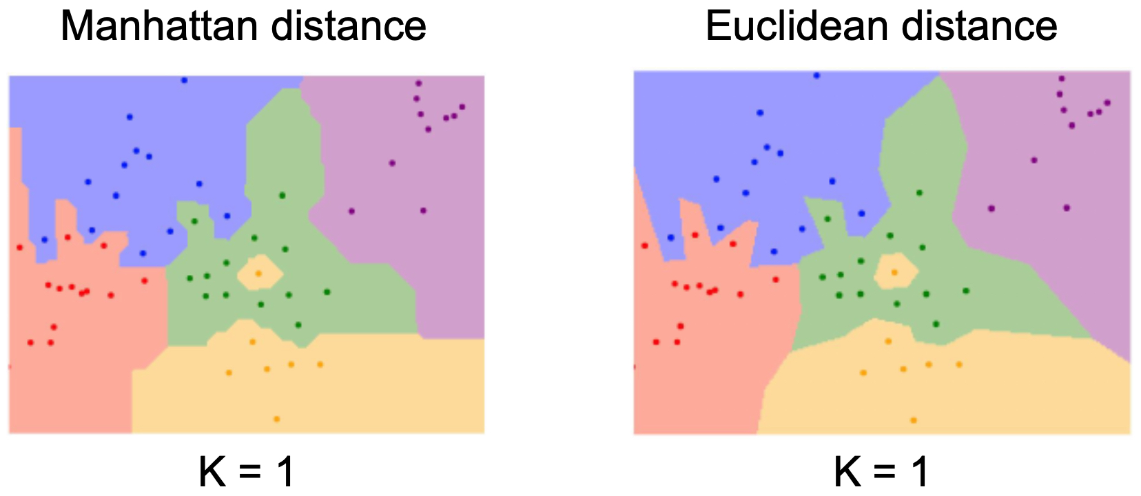
The following figure shows how the choice of distance metric (Euclidean vs. Manhattan) changes the resulting decision boundaries:
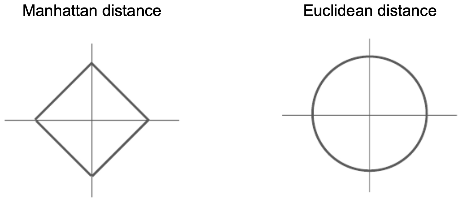
- The following figure illustrates the geometry of these metrics: L1 (Manhattan) equidistant points form a diamond, while L2 (Euclidean) equidistant points form a circle:
Training and Evaluation
-
KNN is a non-parametric model: it does not learn parameters such as weights, but instead memorizes the training set. This leads to several challenges:
- If \(K=1\), the classifier is highly sensitive to mislabeled or noisy training points.
- If \(K\) is too large, predictions are dominated by distant or irrelevant neighbors.
-
Choosing the best value of \(K\) is a hyperparameter optimization problem. To do this properly, the dataset is typically split into:
- Training set: used to store labeled examples.
- Validation set: used to tune hyperparameters such as \(K\) or the choice of distance metric.
- Test set: used only once, after hyperparameters are chosen, to evaluate generalization.
-
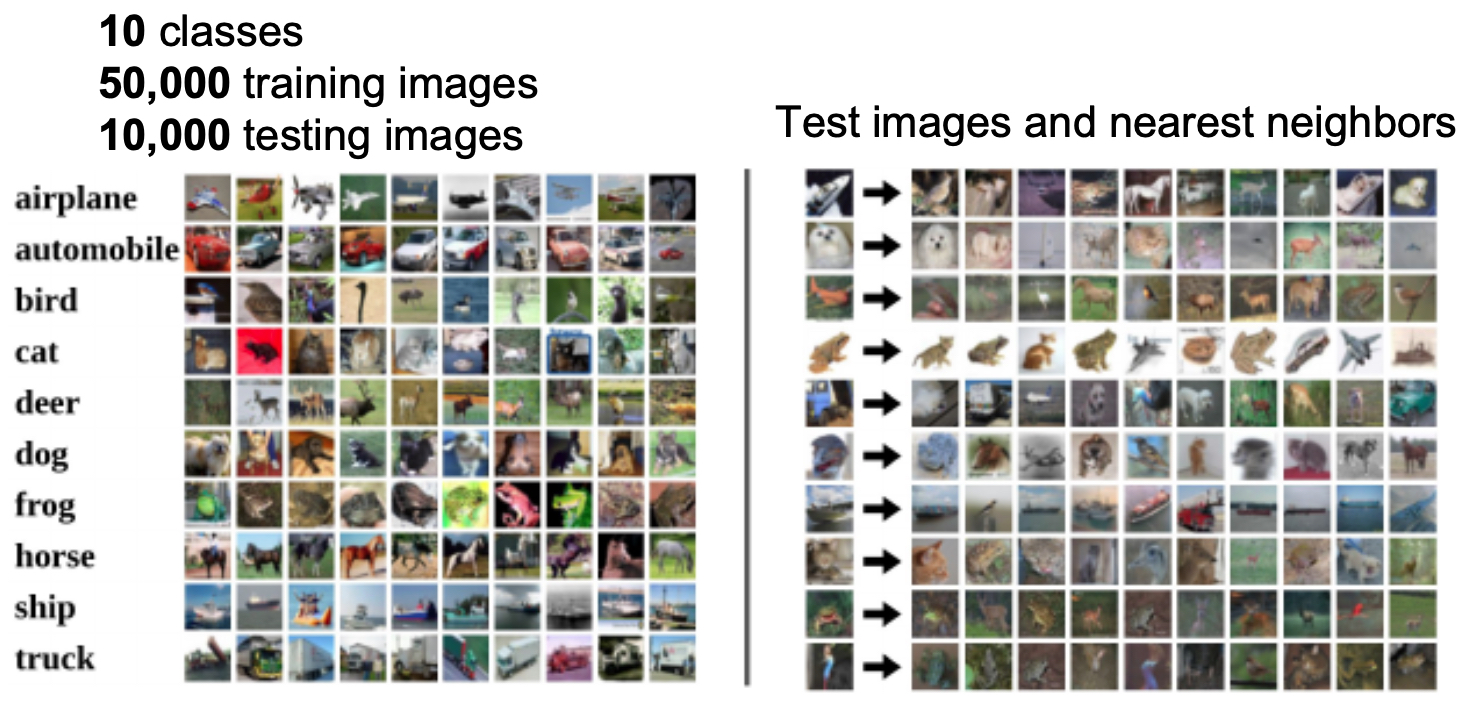
The following figure illustrates this process using the CIFAR-10 dataset, where test images (left) are matched to their nearest training images (right). Classification is determined by majority vote:
- In addition to train/validation/test splits, another common approach is cross-validation, where the dataset is partitioned into K folds. The model is trained on K-1 folds and validated on the remaining one, cycling through all folds. Cross-validation provides robust performance estimates but is rarely used in deep learning due to computational cost.
Decision Boundaries with varying \(K\)
-
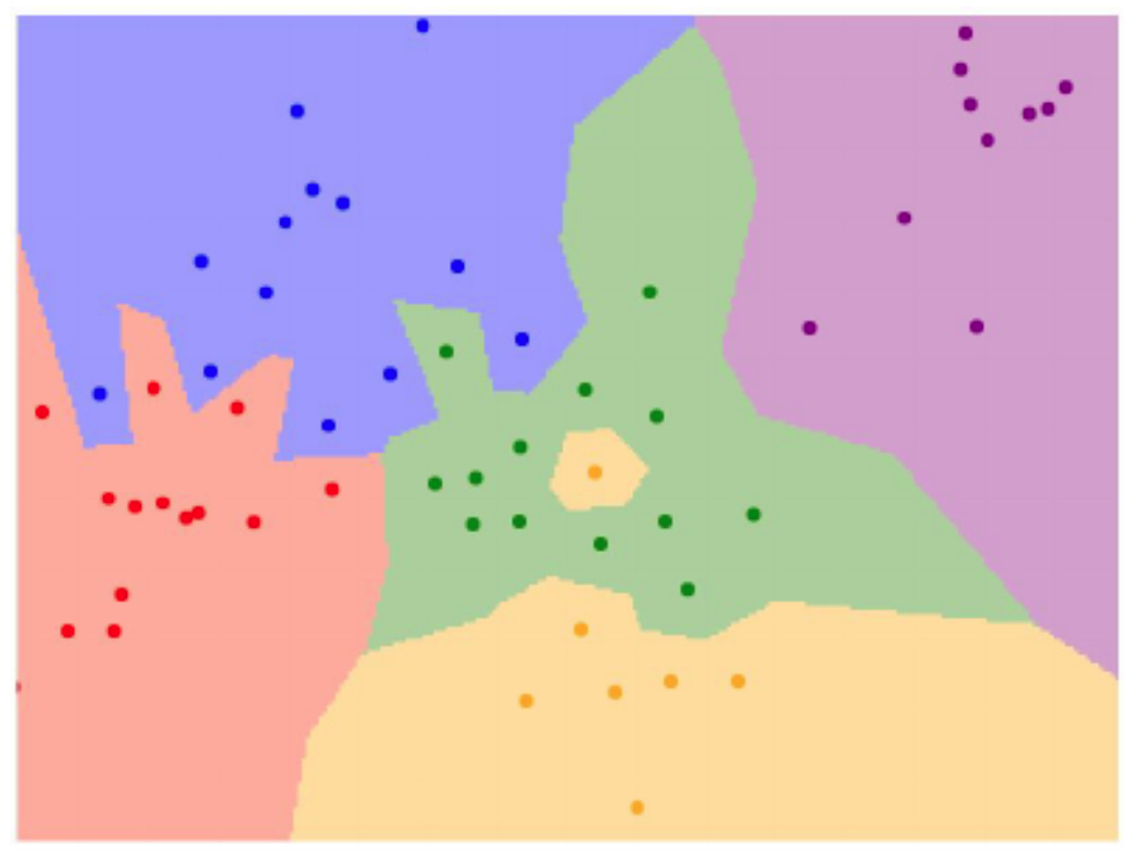
To better understand KNN, it helps to visualize it on a simple 2D dataset with three classes. Each data point is a colored dot, and the classifier assigns labels based on neighbor voting.
-
The figure below illustrates KNN in with the dots representing training instances and the colored regions representing the predictions given if a point were to be tested in that region.
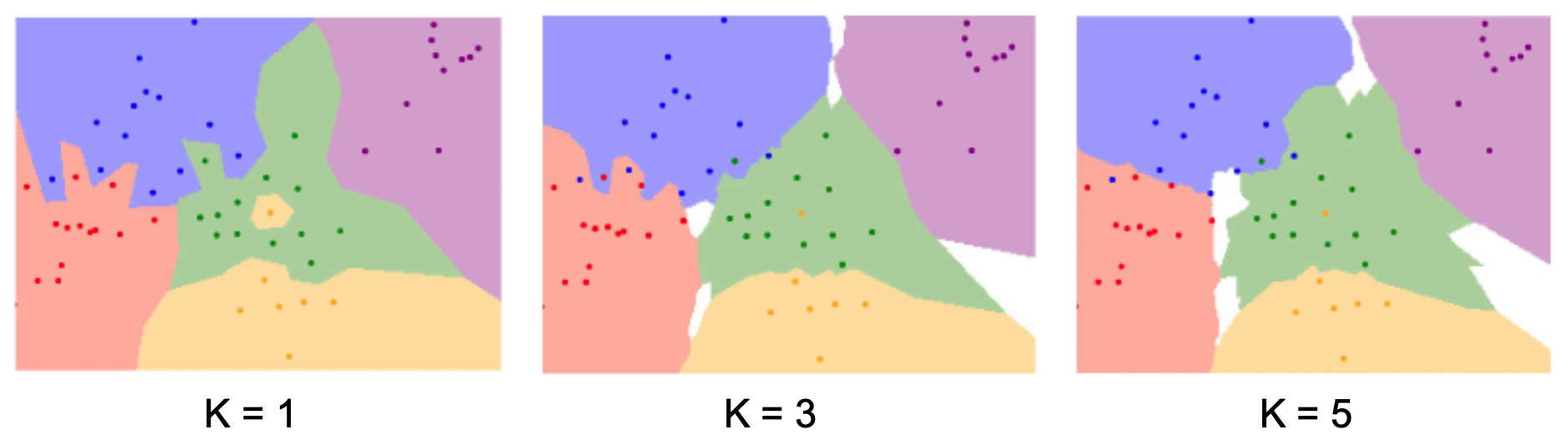
- The figure below illustrates the fact that when using a small \(K\), decision boundaries become very sharp, essentially memorizing the training data. In other words, the figure demonstrates overfitting when using 1-nearest neighbor. The regions are tightly bound to training examples, creating sharp decision boundaries. However, increasing \(K\) smooths the boundaries, improving generalization. Hence, \(K=3\) or \(K=5\) produces softer, more robust decision regions. With even more complex data distributions, the resulting boundaries can take on irregular, jagged forms. This flexibility is a strength of KNN, but it also means performance is highly dataset-dependent. The following figure shows how KNN adapts to such scenarios, though at the cost of interpretability.
Curse of dimensionality
- KNN suffers heavily from the curse of dimensionality. As input dimensionality grows, distances between points become less meaningful.
- For example, consider a relatively small image of size \(128 \times 128 \times 3\) (RGB). Each pixel can take 256 values, leading to roughly \((128 \times 128 \times 3) \times (256 \times 256 \times 256) \approx 8.25 \times 10^{11}\) possible unique images. Even with large datasets, the training set can cover only a vanishingly small fraction of this space. As a result, nearest neighbors found in high dimensions may not be semantically meaningful.
Strengths and Limitations
-
Strengths:
- Simple and intuitive to implement.
- No explicit training cost beyond storing examples.
- Naturally handles multi-class classification.
- Works well for low-dimensional problems.
-
Limitations:
- Scalability: prediction requires distance computations against all training samples, which is prohibitive for large datasets like ImageNet (Deng et al., 2009).
- Curse of dimensionality: in high dimensions, distances lose interpretability.
- Storage cost: requires keeping the entire training set.
- Lack of interpretability: decision boundaries are irregular and dataset-dependent.
-
Despite these drawbacks, KNN remains a valuable teaching tool. It illustrates the principles of data-driven learning, hyperparameter tuning, and the tradeoff between memorization and generalization. More importantly, it serves as a bridge to parametric models such as linear classifiers, which compress training data into compact parameters and provide faster inference.
Linear classifiers
-
While K-nearest neighbors offers a simple data-driven approach, it scales poorly to large datasets because every new test image must be compared with all training images. This inefficiency motivates parametric models, which compress knowledge from training data into a fixed set of parameters. Once trained, such models can classify new images much faster. One of the simplest yet powerful parametric approaches is the linear classifier.
-
A linear classifier maps an input image \(x\) (flattened into a vector) to a vector of class scores using weights \(W\) and biases \(b\):
\[f(x, W, b) = Wx + b\]- where,
- \(x \in \mathbb{R}^D\) is the input image reshaped into a \(D \times 1\) vector (e.g., a \(32 \times 32 \times 3\) image becomes \(D=3072\)).
- \(W \in \mathbb{R}^{C \times D}\) is the weight matrix, where each row corresponds to one of the \(C\) classes.
- \(b \in \mathbb{R}^C\) is the bias vector, shifting the decision boundaries independently of pixel values.
- The output \(f(x, W, b) \in \mathbb{R}^C\) is a vector of class scores.
- where,
-
This is efficient to compute: only a matrix multiplication and a vector addition.
-
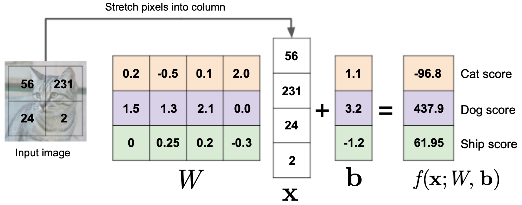
The following figure illustrates a toy version of a linear classifier on a tiny 2×2 RGB image with three classes (cat, dog, ship). Each pixel value contributes to the weighted score for each class:
Intuitive interpretation
-
A helpful way to interpret the weight matrix \(W\) is as a set of templates or class prototypes. Each row of \(W\) can be reshaped back into an image, forming an “average” representation of a class. When computing the dot product \(Wx\), the model measures the similarity of the input image \(x\) to each class template. The higher the score, the more similar the input is to that class.
-
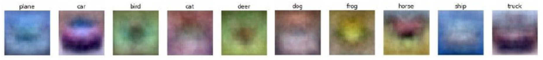
The following figure shows a real example: after training on CIFAR-10, each row of \(W\) produces an activation map that highlights which pixels most strongly drive classification for each category. These resemble crude templates:
-
This interpretation highlights both the power and the limitations of linear classifiers:
- Power: If data is linearly separable in pixel space (i.e., classes can be divided by a hyperplane), the linear classifier works well.
- Limitation: Real-world data is rarely linearly separable. A single template per class cannot capture intra-class variability (e.g., different dog breeds or car models).
-
The bias vector \(b\) further adjusts class preferences by shifting decision scores globally.
Learning the parameters: the loss function
- The challenge lies in learning good values of \(W\) and \(b\). This is done by minimizing a loss function that measures discrepancy between predicted scores and true labels:
-
Two widely used losses for linear classification are:
- Multiclass SVM loss (Cortes & Vapnik, 1995), which enforces margins between correct and incorrect classes.
- Cross-entropy loss with softmax normalization (Goodfellow et al., 2016), which interprets outputs as probabilities.
-
Optimization is typically done with gradient descent or its variants (SGD, Adam). The gradients of the loss with respect to \(W\) and \(b\) guide updates, iteratively improving classification.
-
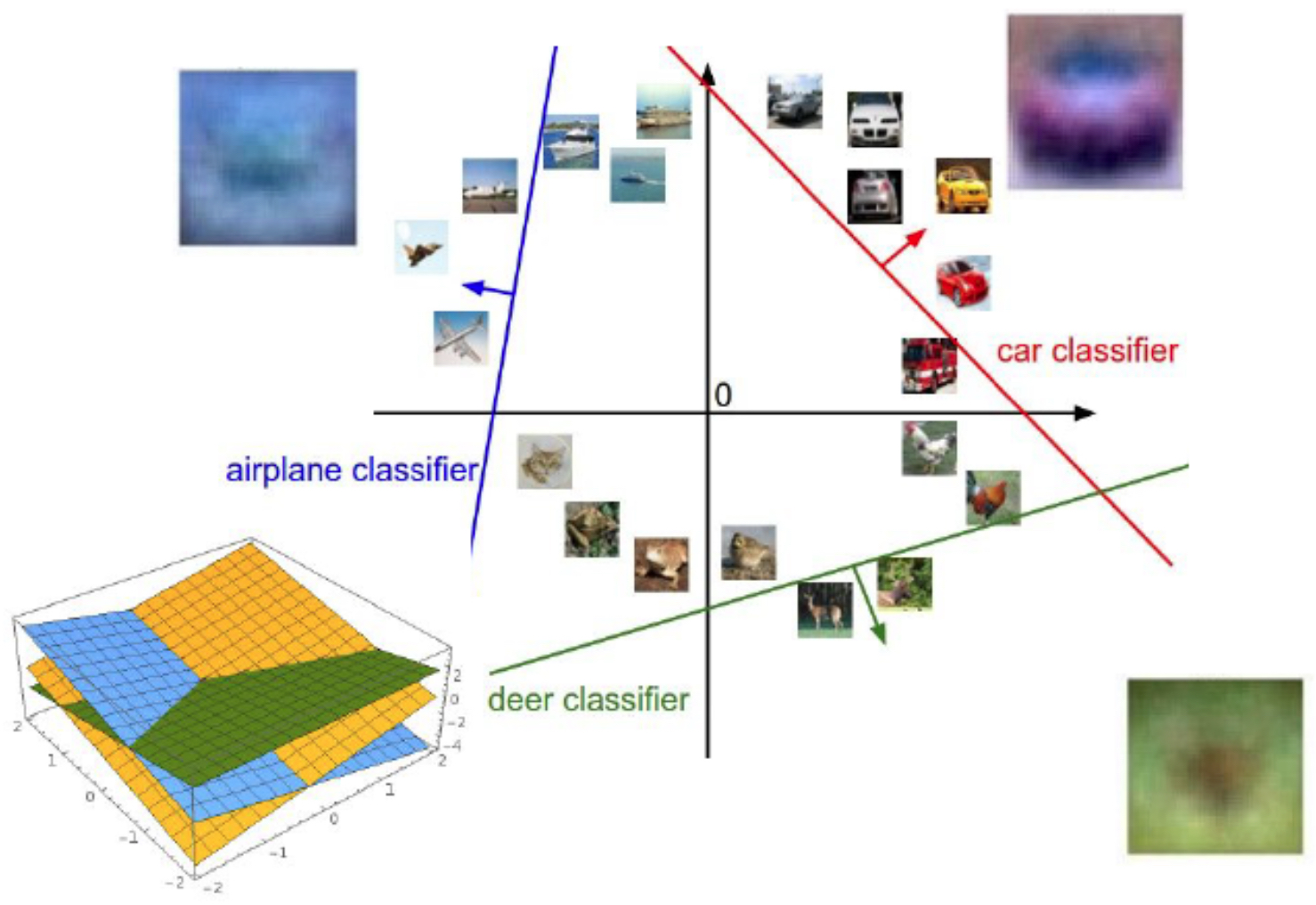
The following figure illustrates the concept geometrically: linear classifiers learn hyperplanes that separate different classes in feature space. A new test point is classified according to which side of the hyperplane it falls on:
The limitation of linear decision boundaries
-
If we plot each pixel of an image in its own dimension, the linear classifier carves the space into regions with hyperplanes. This works well only if the data can be separated linearly.
-
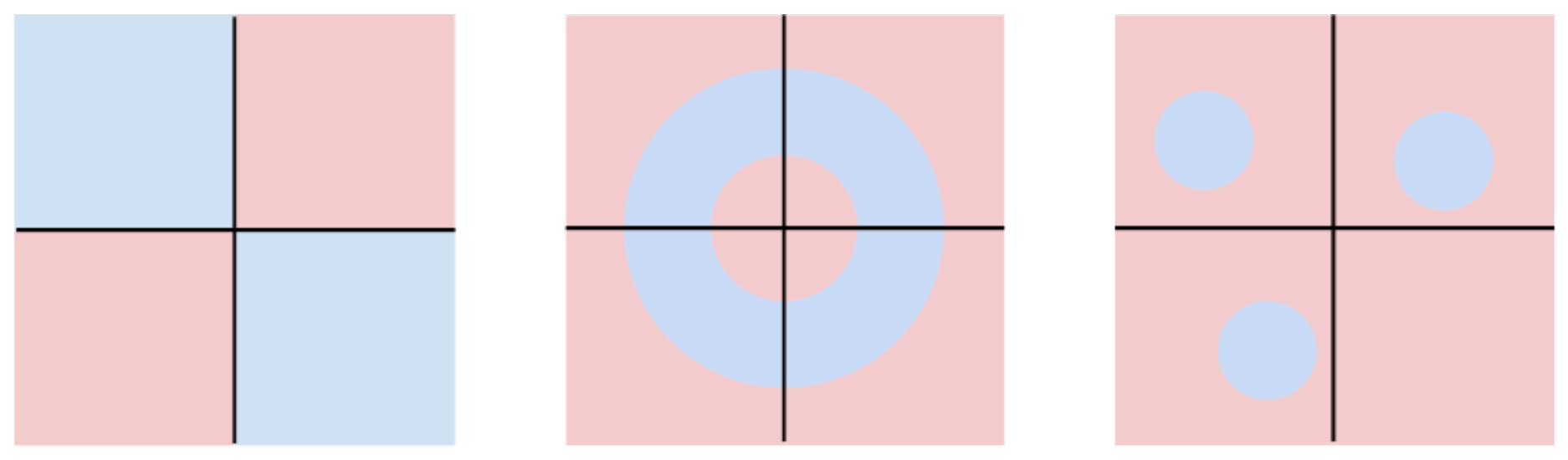
The following figure illustrates this limitation: two classes (blue vs. pink) are separated by a nonlinear boundary. A linear classifier fails to distinguish them:
-
This is a fundamental shortcoming, as many real-world vision tasks involve highly nonlinear relationships between pixels and labels. Factors such as shape, pose, viewpoint, and background often cannot be separated with a single linear hyperplane.
-
These limitations directly motivated the development of neural networks, which extend linear classifiers by stacking multiple layers and introducing nonlinear activation functions. With enough layers, neural networks can approximate arbitrarily complex functions (Hornik, 1991).
Takeaways
- Linear classifiers compress training data into a fixed weight matrix \(W\) and bias vector \(b\).
- They offer fast inference compared to KNN.
- They are interpretable in terms of class templates.
- Their main limitation is linearity: they fail when data is not linearly separable.
-
They serve as the building block of neural networks.
- The following figure shows a schematic overview: a \(2 \times 2\) image of a cat, dog, or ship is passed through a linear function to produce class scores for each of the three class labels:
- Thus, linear classifiers mark the transition from simple, interpretable models toward the deep neural architectures that now dominate computer vision.
Neural Networks
- The limitations of linear classifiers reveal a crucial insight: real-world visual data often requires nonlinear decision boundaries. To address this, researchers developed neural networks, which extend linear models by stacking multiple layers of linear classifiers with nonlinear activation functions in between. This stacking allows the model to approximate arbitrarily complex functions (Hornik, 1991).
From linear to deep models
- Mathematically, a single-layer linear classifier computes:
- A two-layer neural network introduces an intermediate representation \(h\), with a nonlinearity \(\sigma(\cdot)\):
- This architecture allows the network to build more abstract features from raw pixels. While the first layer might detect simple edges, deeper layers can detect textures, shapes, and eventually entire objects (LeCun et al., 1998).
Biological inspiration
- Neural networks are loosely inspired by the brain’s structure. Each neuron takes inputs, applies a weight and bias, passes the result through a nonlinearity, and outputs a signal to the next layer. While vastly simplified compared to real neurons, this abstraction has proven powerful in modeling perception.
Activation functions
-
The power of neural networks comes from the introduction of nonlinear activation functions, which allow them to model complex decision surfaces. Common choices include:
-
Sigmoid:
- Hyperbolic tangent (tanh):
- Rectified Linear Unit (ReLU) (Nair & Hinton, 2010):
Training neural networks
- Training a neural network involves minimizing a loss function (e.g., cross-entropy loss) using gradient descent. The key innovation is backpropagation (Rumelhart et al., 1986), which efficiently computes gradients of the loss with respect to all parameters by applying the chain rule through the network layers.
Depth and expressivity
- The central insight of deep learning is that stacking multiple layers exponentially increases representational capacity. Shallow networks can model only limited classes of functions, while deeper ones can capture hierarchical structures in data: from pixels → edges → textures → objects.
Takeaways
- Neural networks extend linear classifiers by introducing nonlinear transformations.
- Each layer progressively extracts more abstract features from raw input.
- Backpropagation enables efficient training of networks with many layers.
- Activation functions like ReLU make deep models practical and scalable.
-
By increasing depth, neural networks achieve the expressive power needed for real-world visual recognition.
- This transition from linear classifiers to deep neural networks paved the way for breakthroughs in computer vision, culminating in convolutional neural networks (CNNs), which we explore next.
Convolutional Neural Networks (CNNs)
-
While fully connected neural networks can, in principle, model complex visual decision boundaries, they scale poorly for images. A single 32 × 32 × 3 RGB image already has 3,072 input dimensions; connecting this to even one hidden layer of 1,000 neurons requires over 3 million parameters. For larger images, parameter counts explode, leading to overfitting and inefficiency.
-
Convolutional Neural Networks (CNNs) solve this by leveraging two key ideas:
- Local connectivity: Instead of connecting every pixel to every neuron, CNNs use filters (kernels) that focus on local neighborhoods.
- Parameter sharing: The same filter slides (convolves) across the entire image, drastically reducing parameters while exploiting translation invariance.
-
This architecture makes CNNs far more efficient and well-suited for images, where local patterns (edges, textures) repeat across spatial locations.
The convolution operation
-
Mathematically, a convolution between an input image \(I\) and a filter \(F\) is:
\[S(i, j) = (I * F)(i, j) = \sum_m \sum_n I(i+m, j+n) \cdot F(m, n)\]- where \((i,j)\) indexes spatial locations and \((m,n)\) indexes filter elements. Each output \(S(i,j)\) represents how strongly the filter matches the input region around \((i,j)\).
Pooling layers
- CNNs also use pooling layers (e.g., max pooling, average pooling) to reduce spatial resolution while retaining important features. Pooling introduces invariance to small translations and distortions, which is crucial for robust image classification.
Historical breakthroughs
-
CNNs have a rich history:
- LeNet-5 (LeCun et al., 1998) demonstrated CNNs on handwritten digit recognition, achieving state-of-the-art results on MNIST.
- AlexNet (Krizhevsky et al., 2012) revolutionized computer vision by winning the ImageNet challenge with a massive margin, powered by deeper CNNs, ReLU activations, dropout, and GPU training.
- Successive architectures — VGG (Simonyan & Zisserman, 2015), ResNet (He et al., 2016), and beyond — pushed depth and efficiency further, enabling large-scale recognition.
Hierarchical feature learning
-
One of CNNs’ greatest strengths is their ability to learn hierarchical representations:
- Lower layers detect edges and simple textures.
- Middle layers detect shapes and parts of objects.
- Higher layers detect semantic objects (faces, cars, animals).
Computational considerations
- Parameter efficiency: CNNs reduce parameters by sharing filters, compared to dense fully connected layers.
- Translation invariance: Learned filters generalize across image positions.
-
Hardware acceleration: CNNs map well to GPUs and TPUs due to highly parallelizable convolution operations.
- These properties make CNNs the backbone of modern computer vision systems.
Takeaways
- CNNs introduce convolution and pooling layers to efficiently extract spatial features from images.
- They exploit local connectivity and parameter sharing, dramatically reducing the number of parameters.
- Hierarchical representations allow CNNs to progress from pixels to objects.
- Breakthroughs like LeNet and AlexNet established CNNs as the dominant paradigm in vision.
-
Modern architectures like ResNet and DenseNet push these ideas further, enabling ever deeper and more accurate models.
- CNNs remain the foundation of most state-of-the-art computer vision pipelines, and they pave the way toward more advanced architectures like transformers for vision.
Vision Transformers (ViTs)
- Although CNNs have dominated computer vision for decades, they come with certain limitations: they rely heavily on local convolutional filters and handcrafted design choices such as pooling. Meanwhile, in natural language processing (NLP), transformers (Vaswani et al., 2017) revolutionized the field by relying purely on self-attention mechanisms, without convolutions or recurrence. Researchers soon adapted these ideas to vision, leading to the Vision Transformer (ViT) (Dosovitskiy et al., 2020).
From images to sequences
-
Transformers expect sequential input (like words in a sentence). To use them for images, ViTs divide an image into fixed-size patches (e.g., 16×16 pixels). Each patch is flattened and linearly projected into a vector, then position embeddings are added to retain spatial information.
-
Formally, for an image \(x \in \mathbb{R}^{H \times W \times C}\), it is split into \(N = \frac{HW}{P^2}\) patches of size \(P \times P\), which are then mapped to embeddings:
\[z_0 = [x_{\text{class}}; x_p^1 E; x_p^2 E; \dots; x_p^N E] + E_{\text{pos}}\]- where \(x_{\text{class}}\) is a special classification token, \(E\) is the patch embedding matrix, and \(E_{\text{pos}}\) are positional encodings.
Self-attention mechanism
-
At the core of transformers is the multi-head self-attention mechanism, which allows the model to weigh interactions between all patches:
\[\text{Attention}(Q, K, V) = \text{softmax}\left(\frac{QK^T}{\sqrt{d_k}}\right) V\]- where \(Q, K, V\) are query, key, and value matrices derived from input embeddings, and \(d_k\) is the key dimensionality. This mechanism enables global reasoning: each patch can directly attend to every other patch, unlike CNNs, which only see local neighborhoods.
Hierarchical features: CNNs vs. ViTs
- While CNNs build hierarchy by stacking convolutions, ViTs rely on attention layers to capture both local and global dependencies. Early layers may attend to edges and textures, while later layers focus on object-level structure. Importantly, attention is adaptive: different images induce different connectivity patterns, unlike the fixed filters of CNNs.
Training challenges
-
ViTs were initially found to require very large datasets (e.g., JFT-300M) to outperform CNNs. This is because transformers, unlike CNNs, do not encode strong inductive biases like locality or translation invariance. Subsequent work introduced hybrid models and improved training recipes (e.g., data augmentation, distillation, better optimizers) that made ViTs competitive on smaller datasets such as ImageNet-1k.
-
Notable follow-ups include:
- DeiT (Touvron et al., 2021): Efficient training of ViTs on ImageNet without massive external data.
- Swin Transformer (Liu et al., 2021): Introduced hierarchical attention windows, combining CNN-like efficiency with transformer flexibility.
Performance and interpretability
- ViTs now match or surpass CNNs on many benchmarks (e.g., ImageNet, COCO, ADE20K). They also offer improved interpretability: attention maps reveal which regions the model focuses on, offering insight into its decision process.
Takeaways
- Vision Transformers (ViTs) adapt transformer architectures from NLP to vision by treating images as sequences of patches.
- Self-attention enables global receptive fields from the start, unlike CNNs which rely on local filters.
- ViTs require large-scale data and careful training but have become competitive with — and often superior to — CNNs.
- Variants like DeiT and Swin Transformers improve data efficiency and scalability.
-
Transformers now play a central role in state-of-the-art vision systems, and hybrid CNN-transformer models are increasingly common.
- ViTs represent a paradigm shift: from hand-crafted inductive biases in CNNs to flexible, data-driven architectures where attention mechanisms discover relationships directly from data.
Modern Trends in Vision
-
The trajectory from linear classifiers → neural networks → CNNs → Vision Transformers (ViTs) illustrates how computer vision has evolved toward increasingly flexible and powerful models. Modern research now combines these ideas with three major trends:
- Hybrid architectures that blend CNNs and transformers.
- Self-supervised and unsupervised learning.
- Multimodal models that unify vision and language.
Hybrid CNN-Transformer architectures
-
While pure ViTs offer flexibility, they lack the strong inductive biases (locality, translation invariance) that make CNNs efficient on small datasets. Modern models combine the strengths of both worlds:
- Swin Transformer (Liu et al., 2021) introduces hierarchical attention windows, mimicking CNNs’ locality while maintaining transformer flexibility.
- ConvNeXt (Liu et al., 2022) revisits CNNs with design choices borrowed from transformers, achieving competitive results.
Self-supervised learning
-
Traditional supervised learning requires massive labeled datasets like ImageNet. However, labeling millions of images is costly and often infeasible. Self-supervised learning (SSL) bypasses this by creating pretext tasks that exploit the structure of unlabeled data.
-
Prominent SSL approaches include:
- Contrastive learning (e.g., SimCLR Chen et al., 2020, MoCo He et al., 2020): Learn embeddings by bringing augmented views of the same image closer while pushing apart different images.
- Masked image modeling (e.g., BEiT Bao et al., 2021, MAE He et al., 2022): Mask parts of an image and train the model to reconstruct them, inspired by masked language modeling in NLP.
-
Self-supervision has become the dominant pretraining paradigm, enabling models to leverage billions of unlabeled images and transfer knowledge to downstream tasks.
Multimodal vision-language models
-
A striking modern trend is the unification of vision and language in multimodal models. The core idea is to train models jointly on paired image–text data, allowing them to align visual and linguistic representations.
-
Key breakthroughs include:
- CLIP (Radford et al., 2021): Trained on 400M image-text pairs, learning joint embeddings where images and captions that “match” are close in vector space. CLIP enables zero-shot recognition: a model can classify images into categories simply by comparing them to text prompts.
- ALIGN (Jia et al., 2021) and LiT (Zhai et al., 2022): Scale this paradigm to billions of examples, further improving performance.
- Flamingo (Alayrac et al., 2022) and BLIP-2 (Li et al., 2023): Extend vision-language alignment to generative tasks, enabling image captioning, visual question answering, and beyond.
Toward foundation models
-
Modern vision systems are increasingly trained as foundation models: large-scale pre-trained networks that can be adapted to many downstream tasks with minimal fine-tuning. By leveraging billions of images (with or without labels) and multimodal data, these models achieve remarkable generalization.
-
Examples include:
- DALL·E (Ramesh et al., 2021) and Stable Diffusion (Rombach et al., 2022) for image generation.
- PaLI (Chen et al., 2022) for multilingual vision-language tasks.
- Segment Anything Model (SAM) (Kirillov et al., 2023) for general-purpose segmentation.
Takeaways
- Hybrid CNN-Transformer architectures combine efficiency with flexibility.
- Self-supervised learning unlocks vast unlabeled data, reducing reliance on manual annotation.
- Multimodal models like CLIP align vision and language, enabling zero-shot and generative tasks.
-
Vision is moving toward foundation models, trained on massive datasets and adaptable across domains.
- These trends mark a new era of computer vision: from narrow classifiers trained on specific datasets to general-purpose, multimodal AI systems that perceive and reason about the world across modalities.
Citation
If you found our work useful, please cite it as:
@article{Chadha2020ImageClassification,
  title   = {Image Classification},
  author  = {Chadha, Aman},
  journal = {Distilled Notes for Stanford CS231n: Convolutional Neural Networks for Visual Recognition},
  year    = {2020},
  note    = {\url{https://aman.ai}}
}