CS231n • Deep Learning Hardware and Software

• Overview
  • CPU, GPU, and TPU
• Deep Learning Frameworks
  • PyTorch
  • TensorFlow
• The Software Stack and Optimization
  • CUDA: The Foundation of GPU Programming
  • Benchmarking CUDA Performance
  • OpenCL: A Cross-Platform Alternative
  • Data Transfer Bottlenecks
  • The Layered Ecosystem
• PyTorch in Depth: Autograd and Model Building
  • Autograd and Computational Graphs
  • Defining Models: From Sequential to Custom Modules
  • Training Workflow
  • Visualization and Monitoring
  • Pretrained Models and Transfer Learning
  • Why PyTorch?
• TensorFlow in Depth: From Static Graphs to Keras
  • Keras: The High-Level API
  • Built-In Datasets and Preprocessing
  • Model Compilation, Training, and Evaluation
  • Inspecting Models
  • Integration with TPUs and Deployment
• Performance and Cost-Efficiency Trends
  • FLOPs per Dollar
  • Hardware Comparisons
  • Benchmarks and Optimizations
  • Economic and Research Implications
• Data Pipelines and Efficiency Strategies
  • The Memory Transfer Bottleneck
  • Mitigating Data Transfer Delays
  • Framework-Level Solutions
  • Batch Size and Throughput
  • Data Augmentation and On-the-Fly Processing
  • The End-to-End Pipeline
• Scaling Laws and the Historical Trajectory of Deep Learning
  • The Emergence of Scaling Laws
  • Hardware and Cost as Enablers
  • Historical Progression
  • Implications of Scaling Laws
• Citation

Overview

• Deep learning models, particularly convolutional neural networks (CNNs) and large-scale transformers, require massive computational power. The complexity of these models—often involving billions of parameters—demands specialized hardware for training and inference. This section explores the trajectory from traditional general-purpose CPUs to GPUs and TPUs, as well as the frameworks that make deep learning accessible to researchers and engineers.

• As we will see, the story of deep learning hardware is a story of specialization: from CPUs designed for general-purpose sequential computing, to GPUs designed for highly parallel tasks, and finally to TPUs—application-specific chips optimized for tensor algebra and large-scale matrix multiplications. These developments have been central to enabling the rapid progress of the field.

CPU, GPU, and TPU

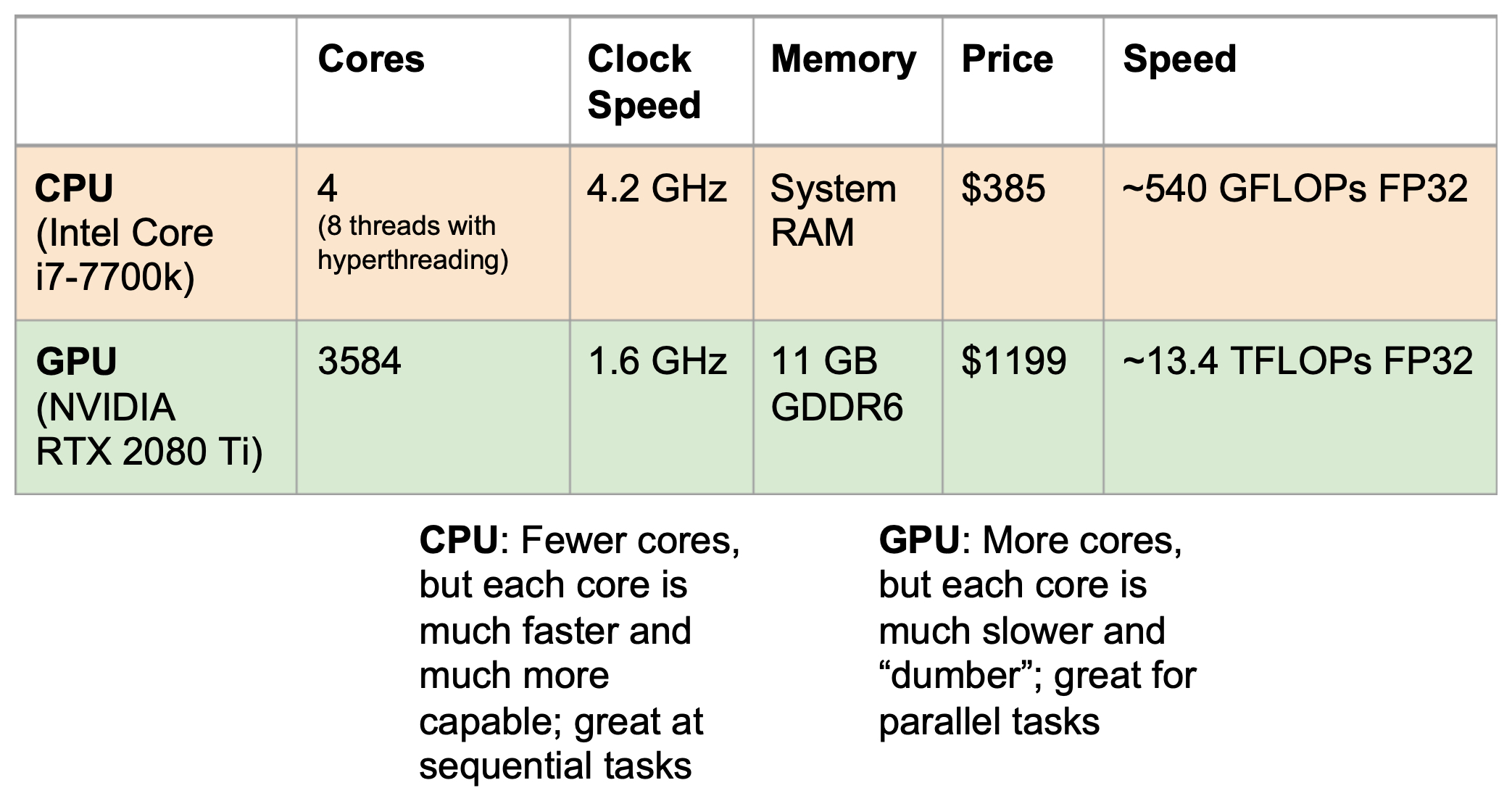
• At the heart of every computing system lies the Central Processing Unit (CPU). CPUs are optimized for sequential tasks: each core is powerful, capable of handling complex operations with high clock speeds. However, they generally have fewer cores, which makes them less effective at highly parallelizable operations like those in deep learning. A typical Intel Core i7-7700k, for example, has 4 cores (8 threads with hyperthreading) running at 4.2 GHz, delivering roughly 540 GFLOPs in single precision (FP32).

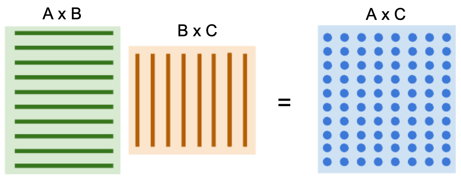
• By contrast, Graphics Processing Units (GPUs) excel at massively parallel tasks. Originally designed for rendering images, GPUs have thousands of smaller, simpler cores. A GPU like the NVIDIA RTX 2080 Ti, with 3584 CUDA cores, runs at 1.6 GHz with 11 GB of GDDR6 memory, offering up to 13.4 TFLOPs FP32 performance. This architecture makes GPUs exceptionally well-suited for the matrix multiplications and tensor operations central to neural networks. For instance, multiplying two matrices involves calculating many dot products between rows and columns, each of which can be computed independently—a task GPUs are tailored for.

• The following figure shows a comparison between a state-of-the-art CPU and GPU, including cores, clock speed, memory, price, and computational throughput.

• The following figure illustrates how matrix multiplication can be decomposed into dot products of rows and columns, a process that is naturally parallelizable and therefore highly efficient on GPUs.

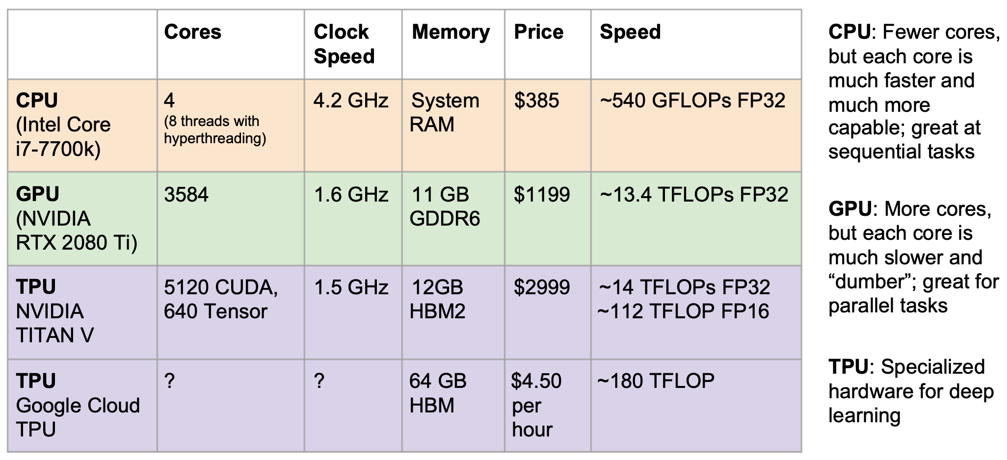
• With the rise of deep learning, GPUs became the hardware of choice. However, as models scaled further, Tensor Processing Units (TPUs) were introduced by Google. TPUs are Application-Specific Integrated Circuits (ASICs) designed explicitly for tensor operations and large-scale deep learning workloads. For example, the NVIDIA Titan V with 5120 CUDA cores and 640 Tensor cores provides ~14 TFLOPs FP32 and ~112 TFLOPs FP16, while Google Cloud TPUs (available on demand at $4.50/hour) offer up to ~180 TFLOPs performance.

• The following figure compares CPU, GPU, and TPU architectures, highlighting their respective trade-offs: CPUs excel at sequential logic, GPUs at parallel operations, and TPUs at specialized tensor operations.

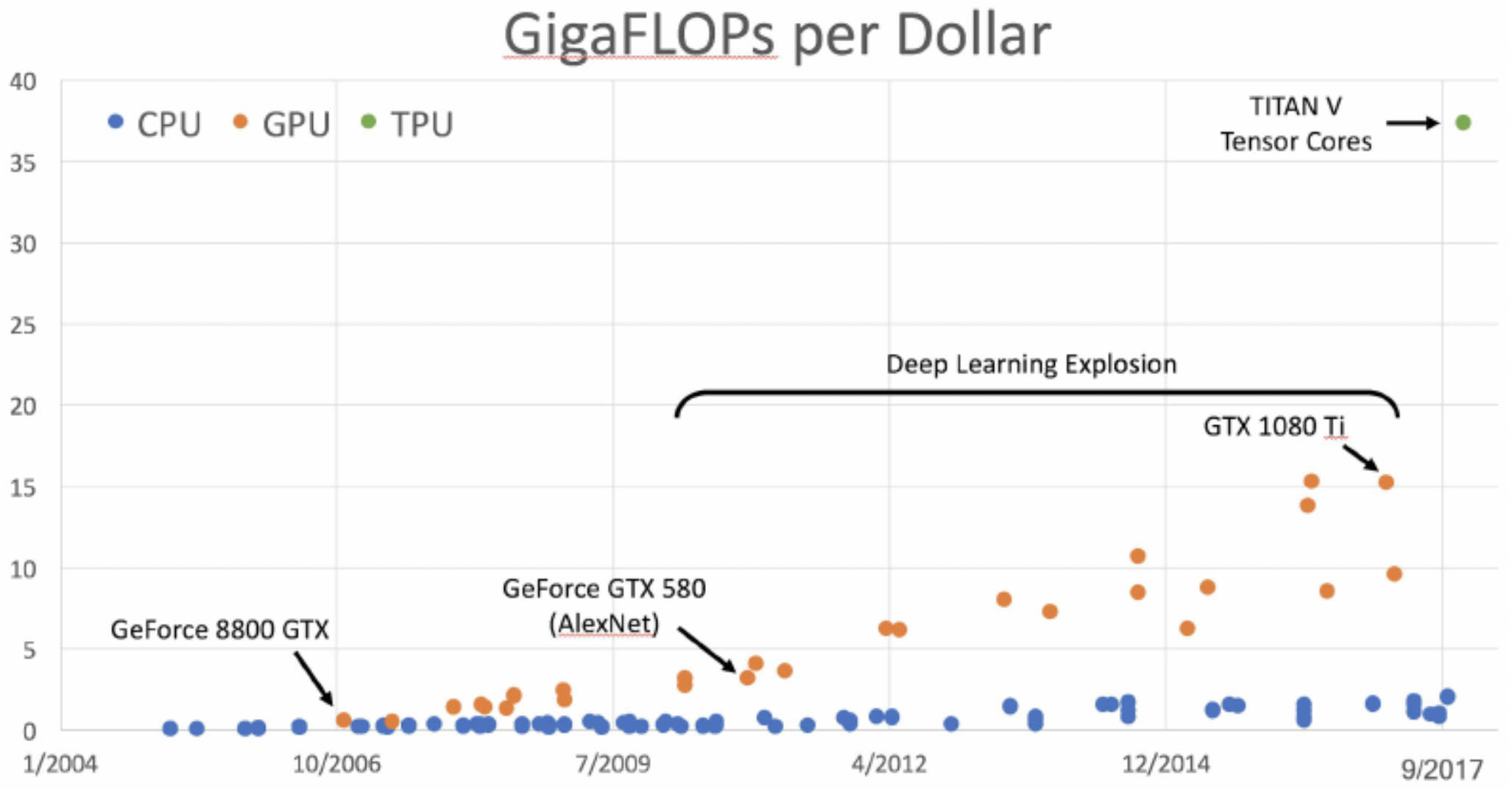
• Another critical metric is cost-efficiency. The number of floating-point operations per dollar (FLOPs/$) has improved dramatically, lowering the economic barrier to training large-scale models.

• The following figure shows how GigaFLOPs per dollar have scaled with the explosion of deep learning.

• To take full advantage of GPUs, low-level programming frameworks like CUDA (developed by NVIDIA) allow writing C-like code that runs directly on the GPU. However, hand-optimizing CUDA kernels is notoriously difficult. Higher-level APIs such as cuBLAS (for linear algebra), cuFFT (for fast Fourier transforms), and cuDNN (for deep neural network primitives) provide optimized routines. These significantly improve performance compared to non-optimized implementations. OpenCL offers a vendor-neutral alternative, but on NVIDIA hardware it is generally slower than CUDA.

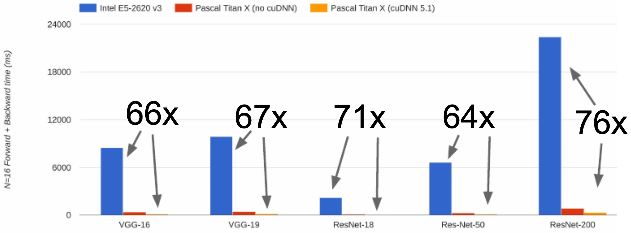
• The following figure presents CNN benchmark comparisons between optimized CUDA code versus a CPU, demonstrating orders-of-magnitude speedups.

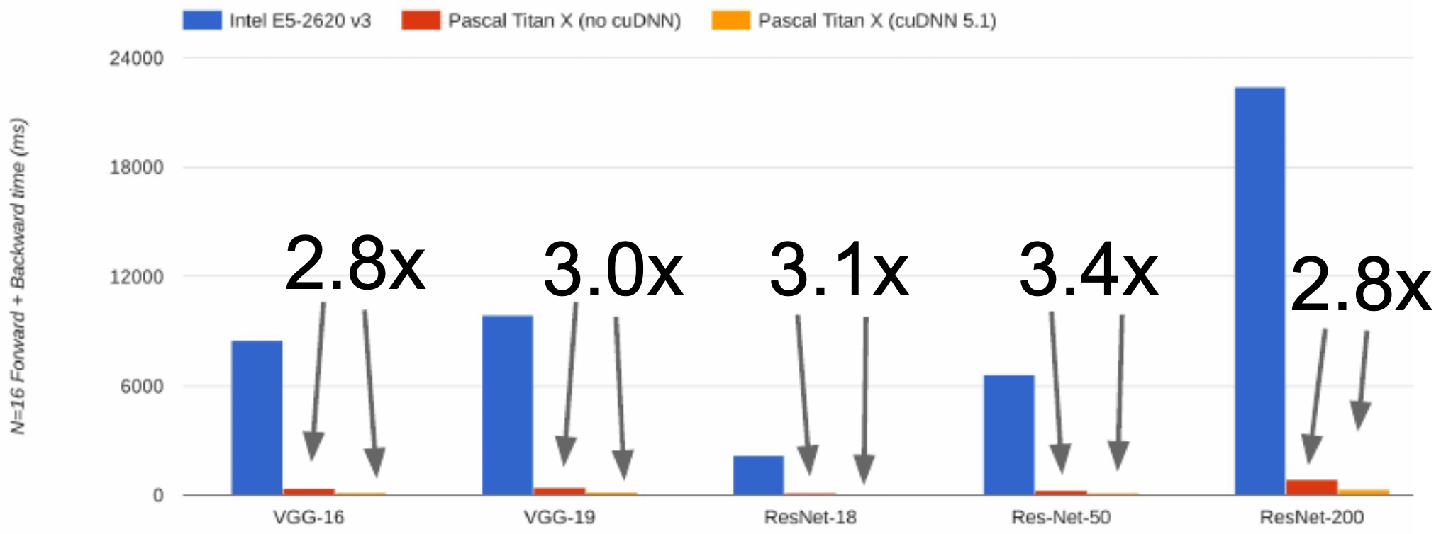
• The following figure presents CNN benchmark comparisons between optimized and non-optimized CUDA code, showing the importance of low-level optimizations.

• Beyond raw computation, practical concerns arise: transferring data between system memory and GPU memory can become a bottleneck. Strategies to mitigate this include preloading data into RAM, using SSDs instead of HDDs, and prefetching data with multithreaded CPU workers.

• These developments highlight a central trend: specialized hardware has been indispensable to deep learning’s success. From CPUs to GPUs to TPUs, each hardware generation has unlocked new possibilities in model scale and complexity.

Deep Learning Frameworks

• The progress of deep learning has been enabled not only by advances in hardware but also by the development of powerful software frameworks. These frameworks abstract away the complexities of writing low-level code for GPUs or TPUs, making it possible for researchers to focus on architecture design, experimentation, and deployment. Instead of manually implementing backpropagation and gradient updates, modern frameworks handle these details automatically through computational graphs and automatic differentiation.

• The primary goals of frameworks such as PyTorch and TensorFlow are to allow researchers to:

  1. Rapidly prototype and test new ideas.
  2. Automatically update network parameters through efficient gradient propagation.
  3. Run seamlessly on GPUs, and increasingly, on TPUs.

• Frameworks represent a critical bridge between high-level model specification and low-level hardware execution. Libraries like CUDA, cuBLAS, and cuDNN remain central, but most practitioners now interact primarily with PyTorch, TensorFlow, or similar frameworks like MXNet (Chen et al., 2015).

PyTorch

• PyTorch, developed by Facebook AI Research (Paszke et al., 2019), has become a favorite among academics and researchers due to its dynamic computation graph and Pythonic design. Unlike static graph frameworks, PyTorch builds computation graphs on the fly, which allows for more intuitive debugging and flexible experimentation. This flexibility has made PyTorch particularly well-suited for tasks in natural language processing and computer vision.

• Originally, PyTorch was created as a GPU-enabled extension of NumPy. Indeed, the syntax between the two is nearly identical. Consider the computational graph for

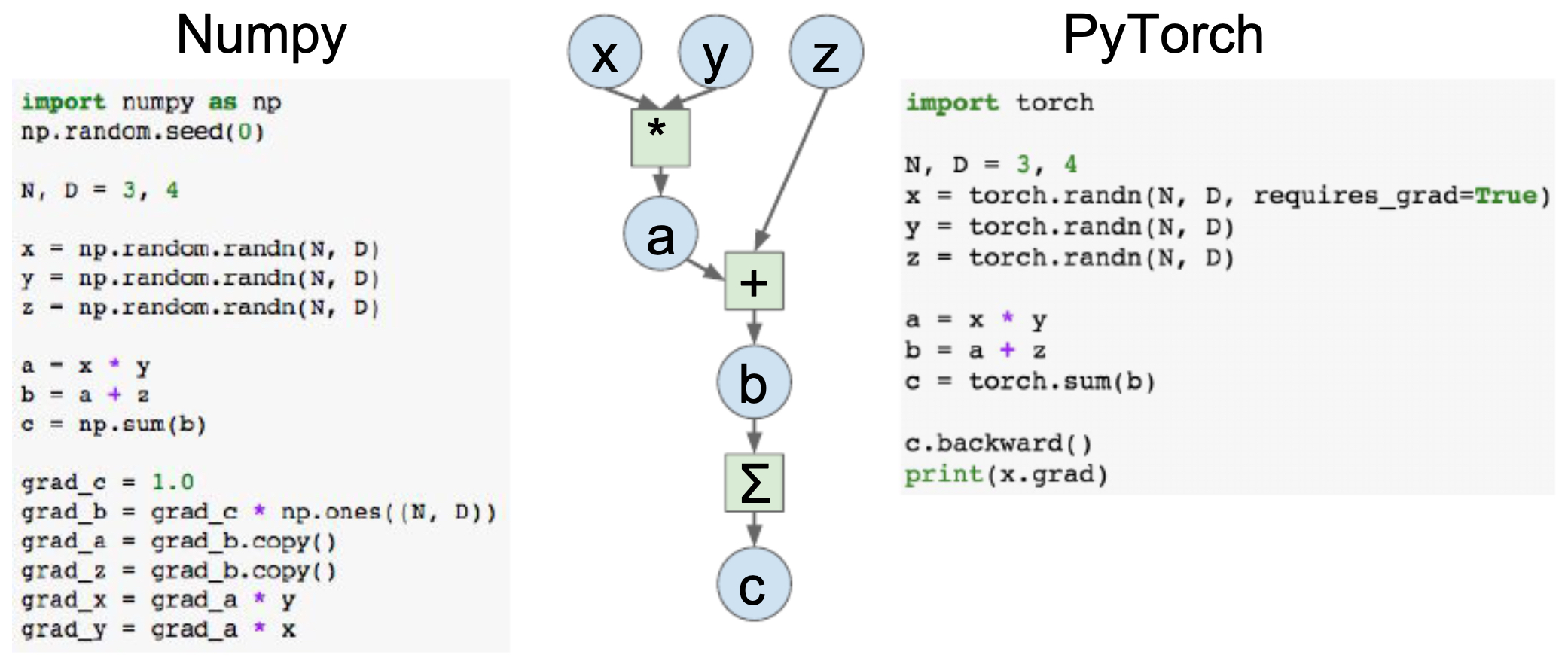
• In NumPy, we must explicitly compute gradients, whereas in PyTorch the autograd engine handles it automatically by setting requires_grad=True.

• The following figure illustrates forward and backward propagation in NumPy versus PyTorch, demonstrating how PyTorch abstracts away much of the manual gradient computation.

• PyTorch also enables seamless GPU acceleration. By simply moving tensors to a CUDA device, computations run on the GPU without further modification. This ease of transition makes PyTorch highly practical for both research and production experiments.

• A major strength of PyTorch lies in its modular design for neural networks. Using torch.nn.Sequential, researchers can define models in just a few lines of code, while custom architectures can be built by subclassing torch.nn.Module. Optimizers such as SGD and Adam are available through torch.optim, reducing the complexity of training loops.

• PyTorch further provides convenient utilities:

• DataLoader and Dataset APIs for batching, shuffling, and multiprocessing.
• torchvision package for pretrained models such as ResNet, VGG, and Inception.

• Visualization tools such as Visdom (for interactive dashboards) and tensorboardX (a TensorBoard wrapper).

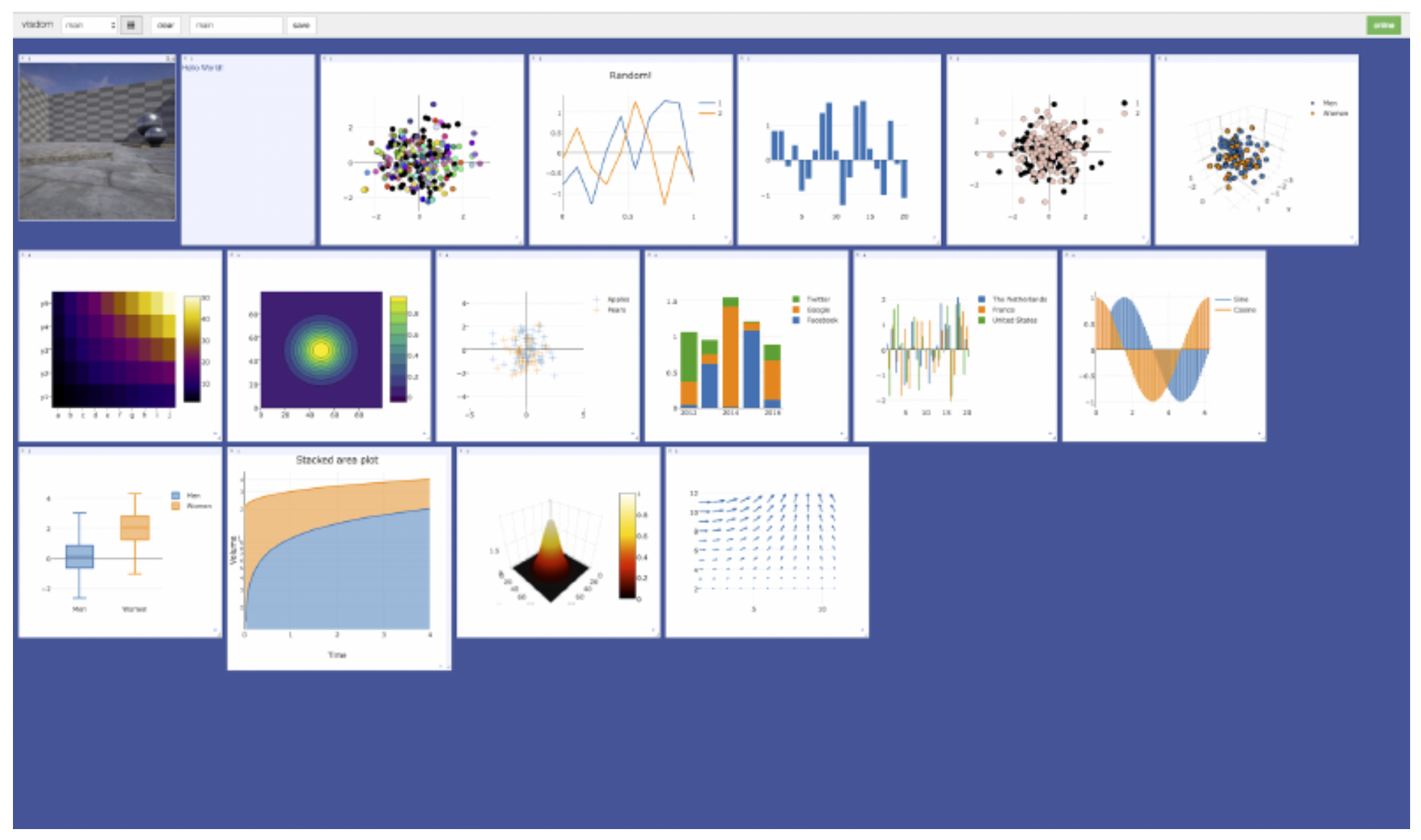
• The following figure shows example interactive visualizations created in PyTorch using the Visdom package.

• Overall, PyTorch’s philosophy is clear: provide a Pythonic, dynamic, and flexible environment for research, while maintaining efficiency at scale.

TensorFlow

• TensorFlow, introduced by Google Brain (Abadi et al., 2016), was designed with scalability and production deployment in mind. Early versions relied on static computation graphs, which enabled compiler-level optimizations such as graph pruning and operator fusion, but made experimentation less intuitive compared to PyTorch. With TensorFlow 2.0, dynamic graph execution (via Eager Execution) became the default, narrowing the usability gap with PyTorch.

• TensorFlow integrates tightly with Google’s cloud ecosystem and TPUs, making it particularly strong for large-scale industrial applications. Its high-level API, Keras, provides a user-friendly, modular interface for constructing networks. A simple model can be created using Sequential, while more complex architectures can be defined with the Model class.

• TensorFlow/Keras also provide built-in datasets such as MNIST, CIFAR-10, and IMDB, making it easy to experiment without additional data preprocessing.

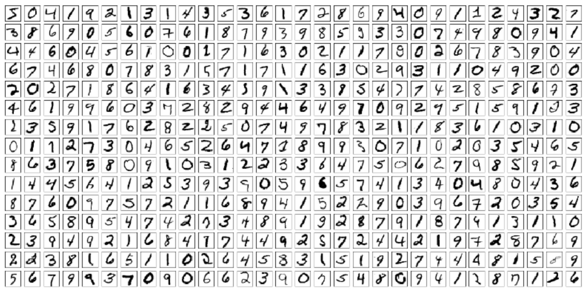
• The following figure shows a visualization of the MNIST dataset using TensorFlow/Keras utilities and Matplotlib. Here, the first 450 training images are displayed in a grid.

• Once data is prepared, TensorFlow models can be compiled with optimizers (e.g., Adam), loss functions (e.g., cross-entropy), and metrics (e.g., accuracy). Training then proceeds with model.fit(), while evaluation uses model.evaluate(). This makes TensorFlow/Keras particularly appealing for practitioners entering the field. Excellent — let’s now build out the Software Stack & Optimization section. I’ve integrated the higher-level treatment from primer1 with the detailed discussion from primer2 (CUDA, cuBLAS, cuFFT, cuDNN, OpenCL, and data transfer bottlenecks). Image placeholders are retained in sequence with richer cover lines.

The Software Stack and Optimization

• While CPUs, GPUs, and TPUs provide the raw computational horsepower for deep learning, it is the software stack that enables this hardware to be used efficiently. Modern deep learning frameworks such as PyTorch and TensorFlow sit at the top of this stack, abstracting away hardware-specific complexities and providing researchers with accessible APIs. Underneath these frameworks lies a carefully engineered set of libraries and tools that maximize performance.
• The optimization story of deep learning is not just about raw FLOPs but also about software efficiency and memory management. CUDA and its ecosystem libraries provide the foundation for modern deep learning frameworks, while higher-level APIs democratize access. By abstracting complexity without sacrificing speed, the software stack has enabled rapid progress in AI research and deployment.

CUDA: The Foundation of GPU Programming

• At the lowest level of the stack is CUDA (Compute Unified Device Architecture), NVIDIA’s proprietary parallel computing platform. CUDA allows developers to write C-like code that runs directly on NVIDIA GPUs, unlocking the ability to exploit thousands of cores for parallel workloads.

• However, writing perfectly optimized CUDA kernels is challenging. Even small inefficiencies in memory access patterns or thread synchronization can cause massive slowdowns. To address this, NVIDIA and the broader ecosystem have built higher-level CUDA libraries optimized for common operations:

• cuBLAS – GPU-accelerated implementation of BLAS (Basic Linear Algebra Subprograms).
• cuFFT – Optimized Fast Fourier Transform (FFT) library.

• cuDNN – The CUDA Deep Neural Network library, optimized for primitives such as convolution, pooling, and normalization.

• Deep learning frameworks rely heavily on these libraries. For example, when PyTorch calls a convolutional layer, it delegates the operation to cuDNN, ensuring highly optimized performance without requiring the researcher to manually write CUDA code.

Benchmarking CUDA Performance

• The impact of these optimizations is striking. CNN benchmarks consistently show orders-of-magnitude improvements when running with optimized CUDA kernels compared to CPU-bound implementations. Even within GPU runs, the difference between optimized versus non-optimized CUDA code is significant.

• The following figure shows CNN benchmark comparisons between optimized CUDA kernels and CPU execution, demonstrating the superiority of GPUs for parallelized deep learning tasks.

• The following figure shows CNN benchmark comparisons between optimized and non-optimized CUDA kernels on GPUs, highlighting the necessity of library-level optimizations for practical deep learning workloads.

OpenCL: A Cross-Platform Alternative

• While CUDA is dominant in the NVIDIA ecosystem, OpenCL (Open Computing Language) provides a vendor-neutral programming framework that runs across GPUs from different manufacturers. However, on NVIDIA GPUs, OpenCL implementations typically run slower than CUDA because NVIDIA’s tooling and optimizations are designed first and foremost for CUDA. In practice, deep learning researchers almost exclusively use CUDA when working with NVIDIA hardware.

Data Transfer Bottlenecks

• Even with optimized libraries, deep learning performance is not determined solely by raw compute power. Data transfer between system memory and GPU memory can become a bottleneck if not managed carefully. For instance:

  • Moving large datasets from RAM to GPU VRAM repeatedly can stall training.
  • Disk read speed also matters: using an SSD (rather than an HDD) can significantly reduce input pipeline delays.
  • Prefetching and caching data with multiple CPU threads helps keep GPUs saturated with data, avoiding idle cycles.

• Frameworks like PyTorch and TensorFlow mitigate these issues with DataLoader and tf.data utilities, which handle prefetching, parallel I/O, and on-the-fly data augmentation. This ensures that GPUs spend their time on compute rather than waiting for inputs.

The Layered Ecosystem

• Putting this together, the modern deep learning software stack can be seen as layered abstraction:

  1. Hardware – CPUs, GPUs, TPUs.
  2. Low-level programming – CUDA (NVIDIA) or OpenCL.
  3. Optimized libraries – cuBLAS, cuFFT, cuDNN (specialized primitives).
  4. Framework backends – PyTorch, TensorFlow, MXNet, JAX.
  5. High-level APIs – Keras, torch.nn, HuggingFace Transformers.

• This layered design has been crucial to deep learning’s success. Researchers can experiment with billions of parameters without needing to optimize GPU kernels themselves, while still benefiting from hardware-level performance gains.

PyTorch in Depth: Autograd and Model Building

• While the previous section introduced PyTorch conceptually, it is important to understand why PyTorch has become the dominant research framework. Its success stems from the way it handles automatic differentiation (autograd), flexible model definition, and GPU-first design.

Autograd and Computational Graphs

• In traditional NumPy code, one must manually calculate gradients during backpropagation. PyTorch eliminates this burden through its autograd engine, which dynamically constructs a computational graph as operations are performed. Each tensor can be flagged with requires_grad=True, and PyTorch automatically tracks dependencies so that calling .backward() computes gradients.

• Consider the equation:

• In NumPy, both the forward pass and the gradient calculations must be explicitly implemented. In PyTorch, however, only the forward computation is specified, while gradients are inferred automatically.

• The following figure illustrates the computational graph for forward and backward propagation in NumPy versus PyTorch, demonstrating how PyTorch simplifies gradient handling.

Defining Models: From Sequential to Custom Modules

• PyTorch offers multiple levels of abstraction for defining models:

  1. Low-level (manual gradients) – One can manually implement forward and backward passes for didactic purposes.
  2. Autograd functions – Users can create custom functions by subclassing torch.autograd.Function and specifying forward/backward computations. This is useful for operations not covered by built-in PyTorch layers.
  3. Sequential API – Simple models can be expressed as a sequence of layers (torch.nn.Sequential).
  4. Custom Modules – For complex architectures, subclassing torch.nn.Module allows users to define flexible forward passes while automatically managing learnable parameters.

• This layered approach balances teaching clarity with research flexibility.

Training Workflow

• Training a neural network in PyTorch typically follows a clear loop:

  1. Data Preparation

     • Load datasets using torch.utils.data.Dataset and DataLoader.
     • Supports batching, shuffling, and multiprocessing.

  2. Model Definition

     • Construct using nn.Sequential or a custom nn.Module.

  3. Forward Pass

     • Compute predictions by passing inputs through the model.

  4. Loss Calculation

     • Compute error (e.g., mean squared error, cross-entropy).

  5. Backward Pass

     • Call .backward() on the loss to compute gradients.

  6. Parameter Update

     • Use optimizers from torch.optim (e.g., SGD, Adam) to update weights.
     • Call .zero_grad() after each update to clear accumulated gradients.

• This explicit workflow is one of PyTorch’s pedagogical strengths. It exposes students to the full training loop while still offering abstractions for production use.

Visualization and Monitoring

• PyTorch offers strong ecosystem support for visualization:

  • Visdom: An interactive dashboard for plotting losses, images, and text streams.
  • tensorboardX: A TensorBoard wrapper for PyTorch that enables dynamic graph visualization and training logs.

• The following figure shows example interactive visuals generated using Visdom with PyTorch tensors and NumPy arrays.

• These tools are particularly valuable for monitoring experiments in real time, debugging issues, and communicating results.

Pretrained Models and Transfer Learning

• Through the torchvision package, PyTorch provides direct access to pretrained models such as ResNet, VGG, SqueezeNet, DenseNet, and Inception. These can be used for fine-tuning on custom datasets, greatly accelerating research. Transfer learning has become a central paradigm in modern AI, and PyTorch’s simple APIs (e.g., torchvision.models.resnet18(pretrained=True)) make it accessible to beginners and experts alike.

Why PyTorch?

• In summary, PyTorch stands out because it:

  • Offers dynamic computation graphs, enabling flexible and intuitive experimentation.
  • Provides seamless GPU integration, requiring minimal code changes.
  • Supports both low-level control and high-level abstraction for diverse use cases.
  • Integrates with a broad ecosystem of visualization, pretrained models, and optimization tools.

• This combination explains why PyTorch dominates in academic research and prototype development, while still increasingly being adopted in production systems.

TensorFlow in Depth: From Static Graphs to Keras

• TensorFlow, originally introduced by Google Brain (Abadi et al., 2016), was designed as a production-first deep learning framework. Its initial strength lay in static computation graphs, which allowed compiler-level optimizations such as operator fusion and deployment portability across CPUs, GPUs, and TPUs. However, static graphs also made the framework less intuitive compared to PyTorch’s dynamic execution.

• With TensorFlow 2.0, this gap narrowed significantly. The framework now defaults to Eager Execution, enabling dynamic computation graphs similar to PyTorch, while still retaining the option for graph optimizations when needed. This transition has made TensorFlow more user-friendly, aligning it with the needs of both researchers and industry practitioners.

• TensorFlow’s evolution can be summarized as a move from rigid but highly optimized static graphs to a dynamic, user-friendly ecosystem that emphasizes both scalability and production deployment. Keras simplifies the research workflow, while integration with TPUs and deployment tools makes TensorFlow an attractive choice for enterprise-scale machine learning systems.

Keras: The High-Level API

• TensorFlow’s high-level interface is Keras, which abstracts model building into a modular, Pythonic API. With Keras, defining a neural network often involves just a few lines of code using either:

  • Sequential API: A linear stack of layers.
  • Functional API: A more flexible way to build complex architectures, such as multi-input/multi-output models.

• For example, a two-layer neural network with a ReLU hidden layer and softmax output can be defined as:

from tensorflow.keras import layers, models

model = models.Sequential([
    layers.Flatten(input_shape=(28, 28)),
    layers.Dense(100, activation='relu'),
    layers.Dense(10, activation='softmax')
])

• Keras integrates smoothly with NumPy, allowing direct use of NumPy arrays for training. This lowers the barrier for researchers transitioning from classical machine learning or scientific computing.

Built-In Datasets and Preprocessing

• TensorFlow/Keras provides built-in datasets such as MNIST, CIFAR-10, CIFAR-100, IMDB, and Fashion-MNIST. These can be loaded with a single call (datasets.mnist.load_data()), returning NumPy arrays. Standard preprocessing steps—such as normalizing pixel values to the range \([0, 1]\)—can then be applied to ease optimization.

• The following figure shows the first 450 images of the MNIST dataset displayed in a grid using Matplotlib, illustrating how TensorFlow and Keras make dataset visualization straightforward.

• Visual inspection of training data is a best practice: it helps confirm correct preprocessing and offers intuition about the dataset’s structure.

Model Compilation, Training, and Evaluation

• Once a model is defined, TensorFlow requires it to be compiled with:

  • An optimizer (e.g., Adam, SGD).
  • A loss function (e.g., categorical cross-entropy).
  • Evaluation metrics (e.g., accuracy).

model.compile(
    optimizer='adam',
    loss='sparse_categorical_crossentropy',
    metrics=['accuracy']
)

• Training then proceeds with model.fit(training_data, training_labels, epochs=N), while evaluation is done using model.evaluate(test_data, test_labels). For the MNIST dataset, even a simple feedforward network achieves test accuracy exceeding 97%.

Inspecting Models

• TensorFlow provides introspection utilities such as model.summary(), which prints each layer, its output shape, and the number of parameters. For example, a simple MNIST classifier might report:

  • Flatten layer: 0 parameters.
  • Dense (100 units): ~78,500 parameters.
  • Dense (10 units): ~1,010 parameters.
  • Total: ~79,510 trainable parameters.

• This transparency makes TensorFlow suitable not only for rapid prototyping but also for educational settings, where understanding layer dimensions and parameter counts is critical.

Integration with TPUs and Deployment

• One of TensorFlow’s strongest differentiators is its tight integration with Google Cloud TPUs, making it possible to scale from local GPU experiments to large distributed TPU clusters with minimal code changes. Additionally, TensorFlow offers deployment pathways to mobile (TensorFlow Lite), web (TensorFlow.js), and production pipelines (TF-Serving).

• This end-to-end ecosystem has made TensorFlow the framework of choice in many industrial settings, even as PyTorch has dominated academic research.

Performance and Cost-Efficiency Trends

• The trajectory of deep learning has been driven not only by innovations in algorithms and architectures, but also by improvements in hardware performance and cost efficiency. Scaling laws in deep learning suggest that increases in available compute directly translate into improvements in model quality (Kaplan et al., 2020). Thus, tracking the evolution of performance and cost metrics provides insight into why deep learning has advanced so rapidly in the past decade.

• Performance and cost-efficiency improvements have been as transformative to deep learning as algorithmic breakthroughs. FLOPs per dollar have improved by orders of magnitude, GPUs and TPUs have eclipsed CPUs for parallel workloads, and optimized software stacks have squeezed further gains from hardware. This virtuous cycle of cheaper compute enabling larger models has been a defining factor in the modern AI era.

FLOPs per Dollar

• A key measure of hardware efficiency is the number of floating-point operations per dollar (FLOPs/$). Over the last decade, FLOPs/$ has improved dramatically, reducing the economic barrier to training increasingly large models. For example, GPUs that once delivered gigaflops (GFLOPs) at high costs now deliver teraflops (TFLOPs) at affordable prices, and TPUs extend this trend even further.

• The following figure shows how GigaFLOPs per dollar have scaled with the explosion of deep learning. Notice the steep acceleration beginning in the 2010s, coinciding with the widespread adoption of GPUs for neural networks.

• This trend parallels the economics of Moore’s Law, but with a sharper trajectory driven by the demand for deep learning. It has enabled researchers at both large labs and smaller institutions to train increasingly sophisticated models.

Hardware Comparisons

• To contextualize cost and performance, let us compare representative hardware across CPU, GPU, and TPU classes:

  • CPU (Intel Core i7-7700k): 4 cores (8 threads with hyperthreading), 4.2 GHz, ~$385, ~540 GFLOPs FP32.
  • GPU (NVIDIA RTX 2080 Ti): 3584 CUDA cores, 1.6 GHz, 11 GB GDDR6, ~$1199, ~13.4 TFLOPs FP32.
  • GPU (NVIDIA Titan V): 5120 CUDA cores, 640 Tensor cores, 1.5 GHz, 12 GB HBM2, ~$2999, ~14 TFLOPs FP32, ~112 TFLOPs FP16.
  • TPU (Google Cloud TPU v2/v3): 64 GB HBM, cloud rental ~$4.50/hr, ~180 TFLOPs.

• The differences are striking: GPUs provide over an order of magnitude more compute than CPUs at similar price scales, while TPUs push the frontier further with specialization for tensor workloads.

Benchmarks and Optimizations

• Raw FLOPs are not the only factor. Optimized software stacks can yield massive performance improvements:

  • Optimized CUDA kernels vs CPU – GPUs achieve tens of times faster performance on CNN benchmarks when compared against CPU-only implementations.
  • Optimized vs non-optimized CUDA kernels – Even within GPU usage, fine-tuned libraries such as cuDNN deliver 2–3x speedups compared to naïve CUDA code.

• The following figure shows CNN benchmark comparisons between optimized CUDA code and CPU execution, highlighting the vast hardware advantage of GPUs.

• The following figure shows CNN benchmark comparisons between optimized and non-optimized CUDA code on GPUs, emphasizing the necessity of software-level optimization.

Economic and Research Implications

• The reduction in compute cost has had several critical implications:

  1. Accessibility – Research groups without access to large-scale supercomputers can now train models of significant scale using commodity GPUs or cloud-based TPUs.
  2. Scaling Laws – Studies have shown that model performance improves predictably with more parameters, data, and compute (Kaplan et al., 2020). Cheaper FLOPs have allowed these scaling laws to be exploited in practice.
  3. Industry Competition – Cloud providers (Google, Amazon, Microsoft) compete on cost-effective training infrastructure, driving further optimization.
  4. Algorithmic Innovation – As hardware enabled bigger models, innovations like transformers (Vaswani et al., 2017) flourished, since their training became computationally feasible.

Data Pipelines and Efficiency Strategies

• While raw compute power is critical to deep learning, real-world training often becomes bottlenecked by data movement rather than arithmetic. Even the most powerful GPUs or TPUs can sit idle if they are not fed data at sufficient throughput. Designing efficient data pipelines has therefore become a key consideration in both research and production systems.
• Efficient data pipelines are just as important as raw compute when training deep learning models. By leveraging SSDs, prefetching, parallel loading, and framework utilities like PyTorch DataLoader and TensorFlow tf.data, practitioners can maximize throughput and minimize idle GPU time. As datasets grow larger and models more complex, pipeline optimization will remain a critical determinant of training efficiency.

The Memory Transfer Bottleneck

• Training workloads typically involve multiple layers of memory hierarchy:

  1. Disk Storage (HDD/SSD) – Persistent storage where raw datasets reside.
  2. System RAM – Staging area for data once loaded from disk.
  3. GPU/TPU VRAM – High-bandwidth memory directly accessible by accelerators.

• Moving data from disk to GPU memory is costly relative to compute time. For instance:

  • Reading from an HDD is orders of magnitude slower than from an SSD.
  • Copying large batches repeatedly between CPU RAM and GPU VRAM can dominate runtime if not managed carefully.

Mitigating Data Transfer Delays

• Several strategies are commonly employed to reduce stalls caused by data movement:

  • Preloading into RAM – Keeping frequently used datasets in system memory avoids repeated disk I/O.
  • Using SSDs instead of HDDs – SSDs drastically reduce latency in accessing large image or text corpora.
  • Prefetching with multiple CPU threads – Overlapping data loading with GPU computation ensures that new batches are ready before the accelerator finishes the current step.
  • Pinned Memory – Allocating page-locked memory allows faster host-to-device transfers.

• In modern frameworks, many of these strategies are abstracted away into utilities, making best practices accessible to practitioners.

Framework-Level Solutions

• Both PyTorch and TensorFlow provide high-level APIs to handle efficient data loading:

  • PyTorch DataLoader – Supports batching, shuffling, multiprocessing, and pinned memory flags. Custom Dataset classes allow streaming from large on-disk corpora without exhausting RAM.
  • TensorFlow tf.data – A pipeline abstraction that enables prefetching, shuffling, parallel reading, caching, and on-the-fly transformations. TensorFlow automatically overlaps these with GPU execution when possible.

• These utilities are crucial when training on large datasets such as ImageNet, COCO, or large-scale text corpora used in transformer models.

Batch Size and Throughput

• Another central factor is batch size, which determines how much data is processed per training step:

  • Larger batch sizes improve throughput by better utilizing GPU cores, but require more memory.
  • Smaller batch sizes may improve generalization in some cases (Keskar et al., 2017), but risk under-utilizing hardware.
  • Gradient accumulation strategies can emulate large batch sizes without requiring massive VRAM.

• Optimizing batch size is therefore a trade-off between statistical efficiency and hardware utilization.

Data Augmentation and On-the-Fly Processing

• For domains like computer vision and speech, data augmentation is essential to prevent overfitting. However, augmentations (rotations, cropping, noise addition, spectrogram transforms) can be computationally heavy. Best practices include:

  • Performing augmentations on CPU threads in parallel with GPU training.
  • Using libraries like Albumentations (CV) or torchaudio for efficient transformations.
  • Leveraging GPU-accelerated augmentations (e.g., NVIDIA DALI) for extreme throughput.

• This ensures that augmentations do not create new bottlenecks in the pipeline.

The End-to-End Pipeline

• Modern deep learning pipelines can be conceptualized as:

  1. Storage – Datasets on disk or cloud.
  2. Preprocessing – Normalization, augmentation, tokenization.
  3. Staging – Prefetching and caching into RAM.
  4. Batching – Packing data into GPU-sized batches.
  5. Accelerator Feed – Transferring data into VRAM with pinned memory.
  6. Compute – Model forward pass, backward pass, optimizer updates.

• Each stage must be tuned to ensure accelerators remain saturated with work. In practice, profiling tools (e.g., NVIDIA Nsight, TensorBoard profiler) help identify bottlenecks across these stages.

Scaling Laws and the Historical Trajectory of Deep Learning

• The remarkable progress of deep learning over the past decade cannot be explained by algorithmic innovations alone. Instead, much of the trajectory can be understood through scaling laws: empirical regularities showing that model performance improves predictably as a function of model size, dataset size, and compute.
• Scaling laws provide a unifying perspective on the rapid rise of deep learning. They show that progress has been as much about hardware, cost efficiency, and pipeline optimization as about new algorithms. By making larger models feasible, improvements in compute have enabled the transformer revolution, foundation models, and the current wave of generative AI. Looking forward, scaling laws suggest that unless fundamental bottlenecks in compute, data, or energy are reached, deep learning progress will continue to be driven by scale.

The Emergence of Scaling Laws

• Early studies (Hestness et al., 2017) observed that test error decreases as a power law with increasing training data. More recently, Kaplan et al. (2020) demonstrated that for language models, performance follows smooth power-law scaling in three key variables:

  1. Model size (parameters)
  2. Dataset size (tokens)
  3. Compute (FLOPs)

• These results suggest that deep learning systems do not “saturate” abruptly, but instead continue improving as resources scale, at least until constrained by optimization stability or data availability.

• Mathematically, the scaling relation for loss can be expressed as:

  \[L(N) = L_\infty + k \cdot N^{-\alpha}\]

  • where:

    • \(L(N)\) is the loss at scale \(N\) (parameters, tokens, or FLOPs),
    • \(L_\infty\) is the irreducible loss (Bayes error),
    • \(k\) is a constant,
    • \(\alpha\) is the scaling exponent.

• This empirical law has been validated across multiple domains including vision, language, and reinforcement learning.

Hardware and Cost as Enablers

• Scaling laws can only be exploited when compute and memory resources are available at scale. Improvements in FLOPs per dollar, the advent of GPU/TPU accelerators, and pipeline optimizations have been decisive in making it possible to train models with:

  • Billions of parameters (e.g., GPT-3, with 175B parameters Brown et al., 2020).
  • Datasets with trillions of tokens (e.g., The Pile, curated for large language models).
  • Training runs consuming petaflop-days of compute.

• Without the exponential reduction in cost per FLOP (as shown earlier in Figure 8.1.4), such scaling would have been economically prohibitive.

Historical Progression

• The history of deep learning hardware and model growth reflects a co-evolutionary cycle:

  1. CPUs era (pre-2010) – Early neural networks trained on CPUs, limited to millions of parameters.
  2. GPU era (2012 onward) – The success of AlexNet on ImageNet (Krizhevsky et al., 2012) demonstrated GPUs’ power, enabling deeper CNNs.
  3. TPU era (2016 onward) – Google’s TPUs accelerated tensor workloads and reduced training costs for industrial-scale models.
  4. Foundation model era (2018 onward) – Transformers, combined with GPU/TPU clusters, enabled massive autoregressive models such as BERT (Devlin et al., 2019) and GPT-3.
  5. Current trajectory – Scaling continues, with models like GPT-4 and beyond trained on unprecedented compute budgets, exploiting the predictable gains suggested by scaling laws.

Implications of Scaling Laws

• Scaling laws have several key implications:

  • Predictability – Performance can be forecast in advance, guiding investment in compute resources.
  • Inevitability – As long as compute cost declines, larger models will continue to outperform smaller ones.
  • Data hunger – Training ever-larger models requires not just compute but vast, high-quality datasets.
  • Efficiency research – Work on techniques like mixture-of-experts, sparsity, and retrieval-augmented models aims to “bend” the scaling curve by achieving similar performance at lower compute.

Citation

If you found our work useful, please cite it as:

@article{Chadha2020DeepLearningHWSW,
  title   = {Deep Learning Hardware and Software},
  author  = {Chadha, Aman},
  journal = {Distilled Notes for Stanford CS231n: Convolutional Neural Networks for Visual Recognition},
  year    = {2020},
  note    = {\url{https://aman.ai}}
}