CS231n • CNN Architectures

• Background: CNN Architectures
• AlexNet
  • Key Innovations
  • Architecture
  • Historical Significance
• ZFNet
  • Key Contributions
  • Architecture
  • Historical Impact
• VGGNet
  • Core Contributions
  • Architectures: VGG16 vs VGG19
  • Architectural Comparisons
  • Historical Significance
• GoogLeNet / Inception
  • The Inception Module
  • Computational Cost and Bottleneck Layers
  • Auxiliary Classifiers
  • Overall Architecture
  • Historical Impact
• ResNet
  • The Degradation Problem
  • Core Idea: Residual Learning
  • The Residual Block
  • Training and Optimization
  • Full Architecture
  • Why Residuals Work
  • Historical Impact
• DenseNet
  • Core Contributions
  • Architecture
  • Impact
  • Historical Position
• Additional Architectures
  • Network in Network (NiN)
  • Wide ResNet
  • ResNeXt
  • Stochastic Depth
  • FractalNet
  • SqueezeNet
  • Summary of Additional Contributions
• The Future of CNNs: Efficiency and Beyond
  • Historical Trends
  • Efficient Architectures
  • Hybrid Architectures: Inception-ResNet
  • Looking Ahead
  • Legacy
• Citation

Background: CNN Architectures

• Convolutional Neural Networks (CNNs) have revolutionized computer vision by providing a way to learn hierarchical feature representations directly from raw image data. Their design leverages three key building blocks:

  • Convolutional layers: which apply learnable filters to extract spatial features such as edges, corners, and textures.
  • Pooling layers: which progressively reduce the spatial dimensions while preserving salient information, making computation more efficient and invariant to small translations.
  • Fully connected layers: which map the learned features into decision boundaries for classification tasks.

• The hierarchy of features learned in CNNs progresses from simple local structures in the early layers to increasingly abstract concepts in deeper layers. This architectural innovation makes CNNs particularly suited for tasks like image classification, semantic segmentation, and object detection.

• Over the years, multiple landmark CNN architectures have been proposed, each improving performance, interpretability, and efficiency. Starting with AlexNet in 2012, which first demonstrated the power of deep learning on large-scale datasets, subsequent models such as ZFNet (Zeiler and Fergus, 2014), VGGNet (Simonyan and Zisserman, 2015), GoogLeNet (Szegedy et al., 2015), ResNet (He et al., 2016), and DenseNet (Huang et al., 2017) have fundamentally shaped modern deep learning.

• The following sections provide a detailed exploration of these architectures, situating each within the broader trajectory of CNN development.

AlexNet

• AlexNet, introduced by Krizhevsky, Sutskever, and Hinton in 2012 (Krizhevsky et al., 2012), was the first deep convolutional network to decisively outperform all competitors in the ImageNet Large-Scale Visual Recognition Challenge (ILSVRC). Its impact cannot be overstated: it reduced the top-5 error rate from 26% to 15% (later refined to 16.4% with ensembling), a staggering improvement over prior approaches, and triggered the modern deep learning revolution in computer vision.

Key Innovations

1. Non-linear activation (ReLU) Instead of the traditional sigmoid or tanh, AlexNet used the Rectified Linear Unit (ReLU), which mitigated the vanishing gradient problem and accelerated convergence. This choice directly influenced nearly all subsequent neural network designs.

2. Regularization

   • Dropout regularization with a probability of 0.5 in fully connected layers, reducing overfitting by preventing co-adaptation of neurons.
   • Data augmentation, including random translations and horizontal flips, to artificially enlarge the dataset.
   • L2 weight decay, with regularization hyperparameter set to \(5 \times 10^{-4}\).

3. Normalization AlexNet employed Local Response Normalization (LRN), inspired by lateral inhibition in biological neurons. Though later superseded by batch normalization, it was instrumental in the early success of deep CNNs.

4. Training strategy

   • Optimized with stochastic gradient descent (SGD) with momentum \(\beta = 0.9\).
   • Batch size of 128.
   • Initial learning rate of \(10^{-2}\), reduced manually by a factor of 10 whenever validation accuracy plateaued.
   • To further boost accuracy, the authors trained seven CNN ensembles, lowering the top-5 error from ~18.2% to ~15.4%.

5. Hardware parallelization The network was too large to fit into a single GPU (each available with only 3GB of memory). The authors split the model across two GPUs, assigning half of the neurons to each GPU, with limited cross-GPU communication. This parallel training strategy foreshadowed today’s large-scale distributed training.

Architecture

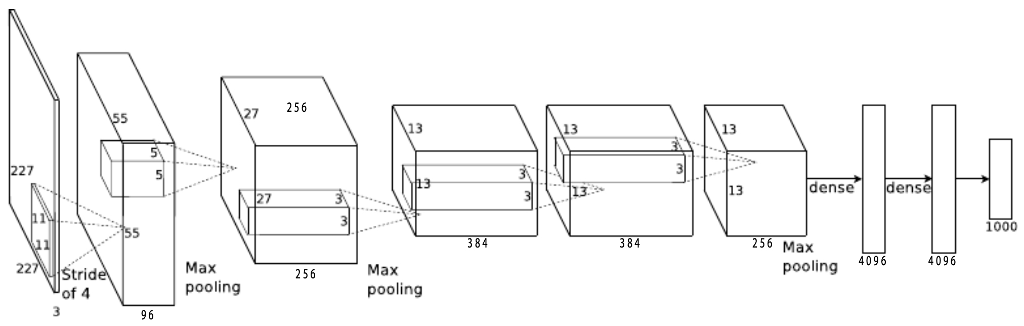
• Structurally, AlexNet consists of 5 convolutional layers followed by 3 fully connected layers, capped with a softmax classifier. Its design is reminiscent of earlier architectures such as LeNet-5 (LeCun et al., 1998), but scaled up dramatically in depth, parameter count, and dataset size. Importantly, it integrated ReLU activations, dropout, and LRN as critical innovations.

• The following figure offers an overview of AlexNet. It highlights the convolutional layers, pooling operations, and fully connected classifier. The simplified diagram shown here condenses the dual-GPU implementation described in the original paper into a single computational pipeline.

Historical Significance

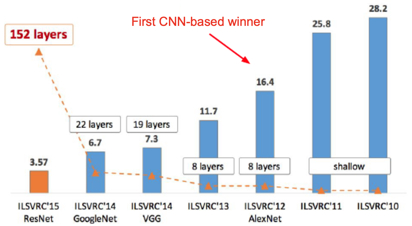
• AlexNet’s success was a turning point for deep learning. For the first time, a CNN decisively won the ImageNet challenge, achieving a 16.4% top-5 error rate compared to the 25.8% of the previous year’s best model.
• This victory established CNNs as the dominant paradigm for computer vision and directly inspired architectures like ZFNet, VGG, GoogLeNet, and ResNet.
• The figure below provides historical context, showing winners of ILSVRC from 2010–2015, with AlexNet as the first CNN-based winner of ILSVRC, setting the stage for the CNN revolution.

ZFNet

• Following AlexNet’s groundbreaking success, researchers asked a critical question: What exactly are CNNs learning inside their layers? This question was answered in 2013 by Matthew Zeiler and Rob Fergus with the introduction of ZFNet (Zeiler and Fergus, 2014), which won the ILSVRC 2013 competition.

• While architecturally similar to AlexNet, ZFNet’s primary contributions were in interpretability and refined design choices that significantly improved both performance and understanding.

Key Contributions

1. Deconvolutional Networks (Deconvnets)

   • Zeiler and Fergus pioneered the use of deconvnets to visualize feature activations.
   • These visualizations projected intermediate feature maps back into pixel space, revealing what each layer was “looking at.”

   • Insights from this method showed:

     • AlexNet’s first-layer filters included not only edge and texture detectors but also high-frequency noise-like patterns.
     • Some filters were poorly tuned and wasted capacity.
   • This interpretability work provided a diagnostic tool, enabling researchers to refine CNN architectures based on what the network was actually learning.

2. Refined Hyperparameters

   • The first convolutional filter was changed from AlexNet’s \(11 \times 11\) with stride 4 to a smaller \(7 \times 7\) with stride 2.
   • This captured more fine-grained spatial information in the early layers.

   • The number of convolutional filters in deeper layers was also increased:

     • Layer 3: from 384 \(\rightarrow\) 512
     • Layer 4: from 384 \(\rightarrow\) 1024
     • Layer 5: from 256 \(\rightarrow\) 512
   • These changes led to more expressive filters and improved representational power.

3. Performance Improvements

   • AlexNet achieved a top-5 error rate of 16.4%.
   • ZFNet lowered this to 11.7% top-5 error rate, a substantial improvement, primarily from better filter design and improved spatial retention.

Architecture

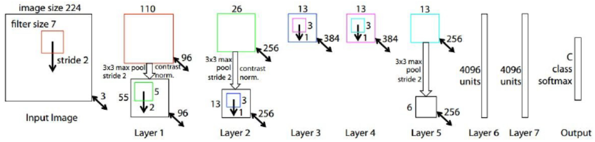
• Structurally, ZFNet retained the same number and ordering of layers as AlexNet (5 convolutional + 3 fully connected). The improvements were primarily in filter sizes, strides, and channel counts.

• The following figure shows the ZFNet architecture, highlighting the progression from convolutional layers to fully connected classification. Compared to AlexNet, the key differences lie in the first convolutional layer and the refinements that yield clearer, more interpretable filters.

Historical Impact

• ZFNet demonstrated two major lessons that profoundly influenced CNN research:

  1. Visualization matters. Neural networks were not black boxes — feature visualization could explain what layers learned, diagnose failures, and guide architectural refinements. This marked the beginning of a broader movement in interpretable deep learning.

  2. Architectural refinements can yield large performance gains. ZFNet was not a radical departure from AlexNet but rather an informed optimization. Yet, this refinement reduced the error rate by almost 5 percentage points on ImageNet, underscoring the importance of thoughtful design.

• Together, these contributions made ZFNet not just a better-performing network but also a scientific lens for understanding CNNs, laying the groundwork for systematic explorations in VGG, GoogLeNet, and beyond.

VGGNet

• The VGG network, introduced by Karen Simonyan and Andrew Zisserman of the Visual Geometry Group at Oxford (Simonyan and Zisserman, 2015), was a landmark step in CNN development. Entered in the ILSVRC 2014 challenge, VGG achieved second place with a top-5 error rate of 7.3%, improving upon ZFNet and demonstrating the power of depth with small filters.

• Although not the most efficient architecture, VGG profoundly influenced subsequent CNN design due to its elegance, systematic construction, and strong performance.

Core Contributions

1. Systematic use of small filters

   • Instead of large convolutional filters such as AlexNet’s \(11 \times 11\) or ZFNet’s \(7 \times 7\), VGG exclusively used stacks of \(3 \times 3\) convolutions with stride 1 and padding 1.
   • Pooling layers were uniformly \(2 \times 2\) with stride 2.
   • Depth was increased significantly — up to 16 or 19 weight layers (VGG16 and VGG19).
2. Effective Receptive Field Expansion

   • Stacking small filters simulates larger receptive fields while maintaining fewer parameters.

   • Two stacked \(3 \times 3\) filters yield a receptive field equivalent to \(5 \times 5\).

   • Three stacked \(3 \times 3\) filters yield a receptive field equivalent to \(7 \times 7\).

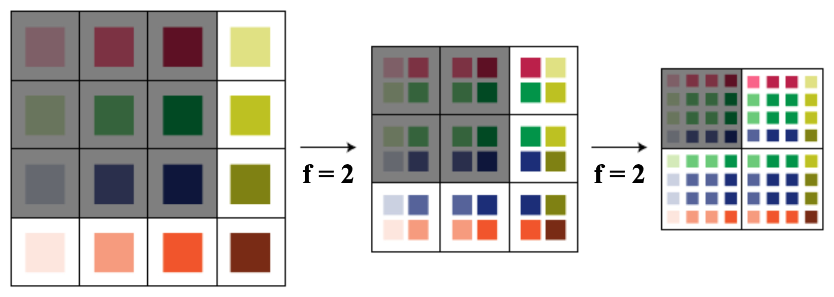
   • In general, if each layer has kernel size \(k\) and stride 1, stacking \(n\) such layers produces an effective receptive field:
   \[k_{\text{eff}} = (k - 1)\cdot n + 1\]
   • For three \(3 \times 3\) convolutions:
   \[k_{\text{eff}} = (3-1)\cdot 3 + 1 = 7\]
   • The following figure illustrates this principle using smaller filters (here with \(2 \times 2\) stacked twice yielding a \(3 \times 3\) receptive field):

   

3. Parameter Efficiency

   • Smaller stacked filters use significantly fewer parameters:

     • A single \(7 \times 7\) filter across \(C\) channels requires \(49C\) weights.
     • Three stacked \(3 \times 3\) filters require \(27C\) weights.
     • Since \(27C < 49C\), VGG achieved efficiency while introducing more non-linearities via additional ReLU activations.
4. Uniform Architecture
   • Unlike AlexNet or GoogLeNet, which used a mix of filter sizes and irregular hyperparameters, VGG employed a clean, homogeneous design: repeating stacks of \(3 \times 3\) convolutions followed by pooling. This simplicity made VGG attractive for transfer learning and practical applications.

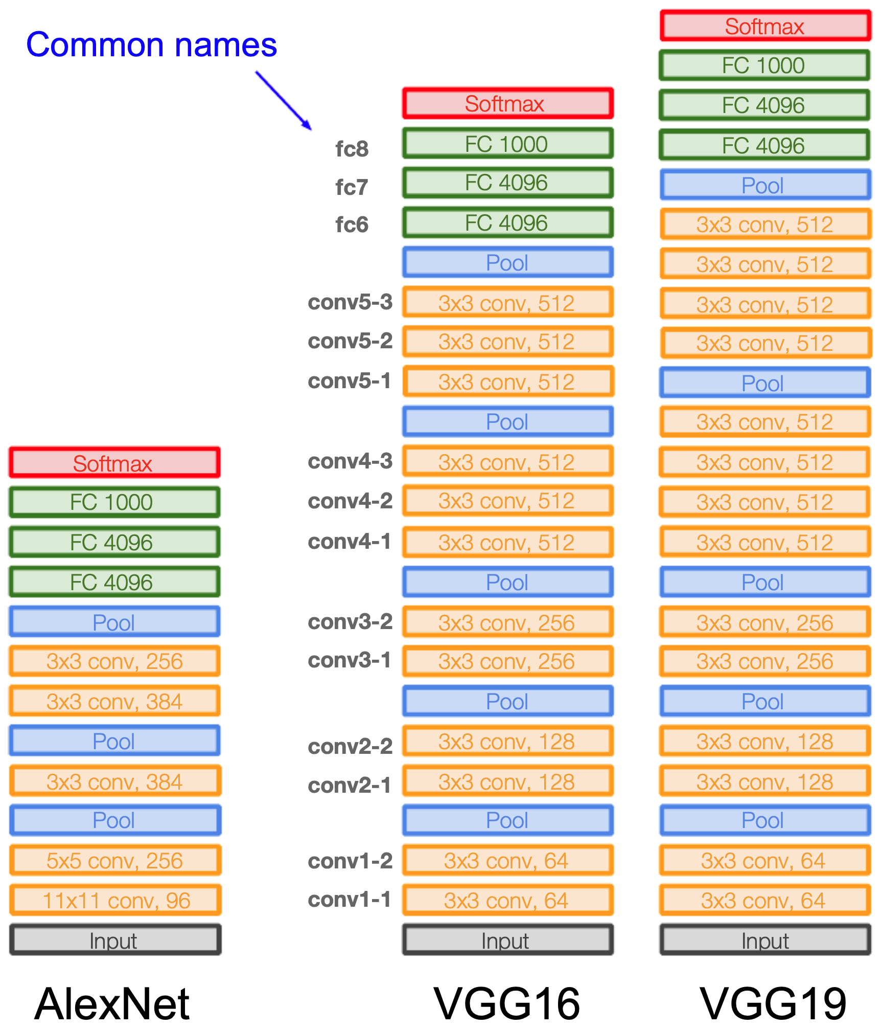
Architectures: VGG16 vs VGG19

• VGG16: 13 convolutional layers + 3 fully connected layers.

• VGG19: 16 convolutional layers + 3 fully connected layers.

• The difference is minor: three extra convolutional layers toward the end of VGG19. Performance improved only slightly, at the cost of higher memory consumption.

• Both networks are considerably deeper than AlexNet’s 8 layers, but they were also computationally expensive — requiring over 138M parameters. This made them slower and more memory-intensive, especially before modern hardware optimizations.

Architectural Comparisons

• The following figure compares AlexNet, VGG16, and VGG19, highlighting how depth was systematically increased in VGG while keeping the filter size small and uniform.

Historical Significance

• VGG proved that depth and small, uniform filters could dramatically improve performance. Although parameter-heavy and inefficient by today’s standards, its simplicity, modularity, and transferability made it one of the most widely used CNN backbones for nearly a decade. VGG’s design became the foundation for countless applications in computer vision, from medical imaging to object detection, until more efficient models like GoogLeNet and ResNet emerged.

GoogLeNet / Inception

• The winner of the ILSVRC 2014 competition was GoogLeNet, introduced by Szegedy et al. (Szegedy et al., 2015). With a top-5 error rate of 6.7%, it outperformed VGG while using far fewer parameters. Its hallmark contribution was the Inception module, which fundamentally changed CNN design by enabling multi-scale feature extraction with high computational efficiency.

The Inception Module

• Instead of committing to a single filter size (as in VGG’s uniform \(3 \times 3\)), GoogLeNet introduced parallel branches of convolutions and pooling within a single module:

  • \(1 \times 1\) convolution (feature reduction, non-linearity introduction)
  • \(3 \times 3\) convolution (mid-scale receptive fields)
  • \(5 \times 5\) convolution (large context capture)
  • \(3 \times 3\) max pooling (local invariance)

• The outputs of all branches were concatenated depth-wise into a single tensor.

• The following figure presents a naïve implementation of an inception module, showing the parallel filter branches (\(1 \times 1\), \(3 \times 3\), \(5 \times 5\), pooling) and their concatenation.

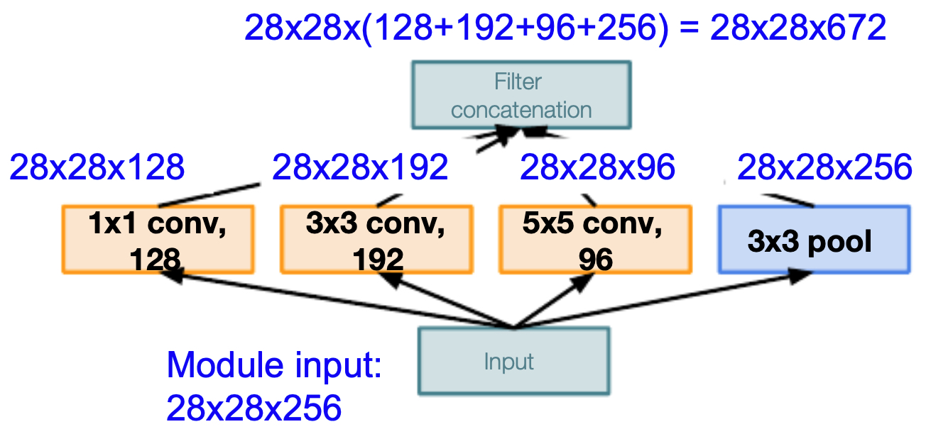
• This design allowed GoogLeNet to capture multi-scale features simultaneously.

Computational Cost and Bottleneck Layers

• Naïvely, large filters like \(5 \times 5\) across many channels lead to prohibitively large parameter counts. As an example:

• For an input of size \(28 \times 28 \times 256\):

  • Applying 192 filters of size \(3 \times 3\) directly requires ~347M operations.
  • Applying 96 filters of size \(5 \times 5\) directly requires ~482M operations.
  • Total cost for the module exceeded 850M operations, which was unsustainable.

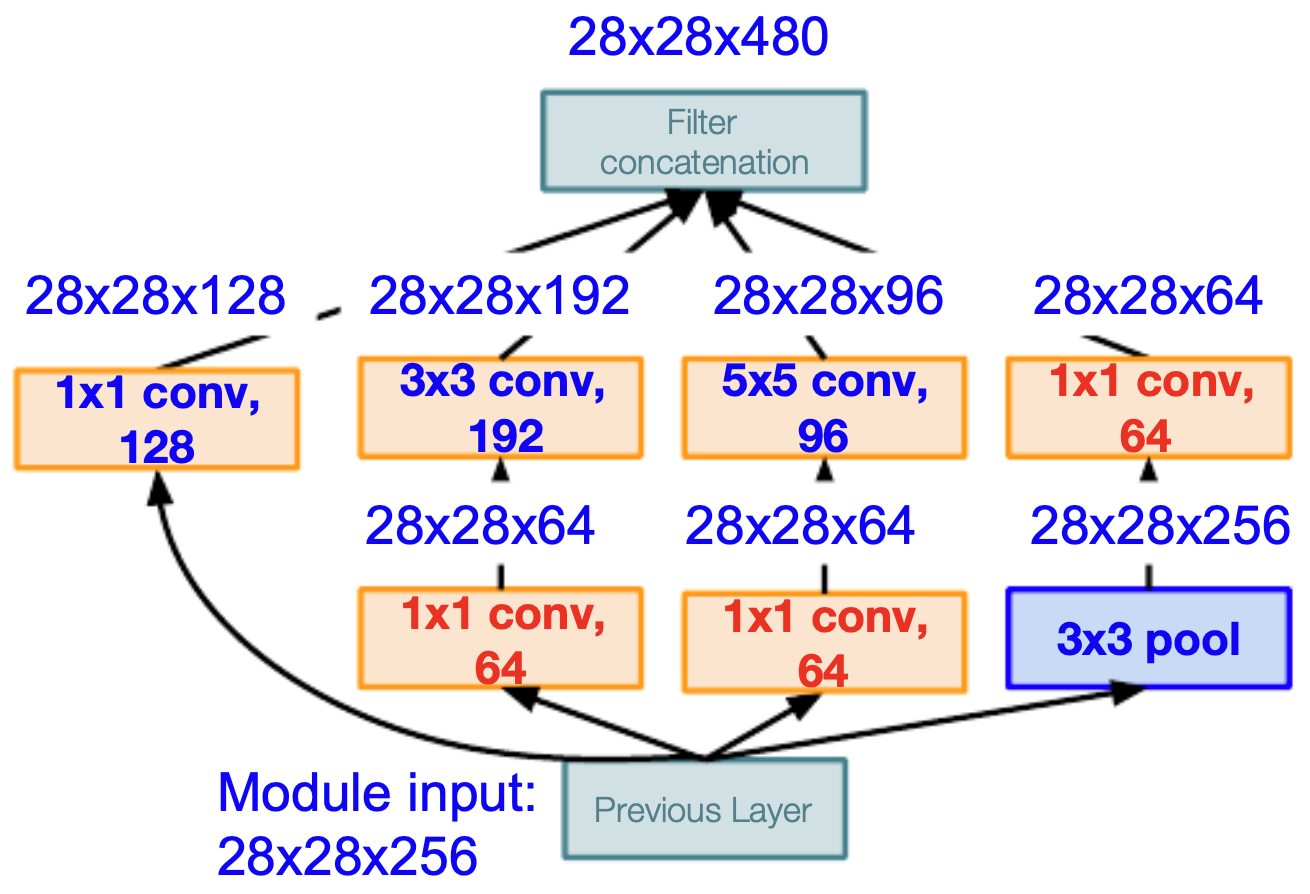
• To address this, GoogLeNet introduced \(1 \times 1\) convolutions as bottleneck layers, reducing the depth before applying costly larger filters.

• For example:

• Since \(C_{\text{red}} \ll C_{\text{in}}\), the parameter cost shrinks dramatically.

• The improved module with \(1 \times 1\) reductions reduced total cost from ~850M to ~260M operations — a 3× efficiency gain without losing expressive power.

• The following figure shows an improved implementation of an inception module by stacking \(1 \times 1\) convolution operations (i.e., “bottleneck layers”).

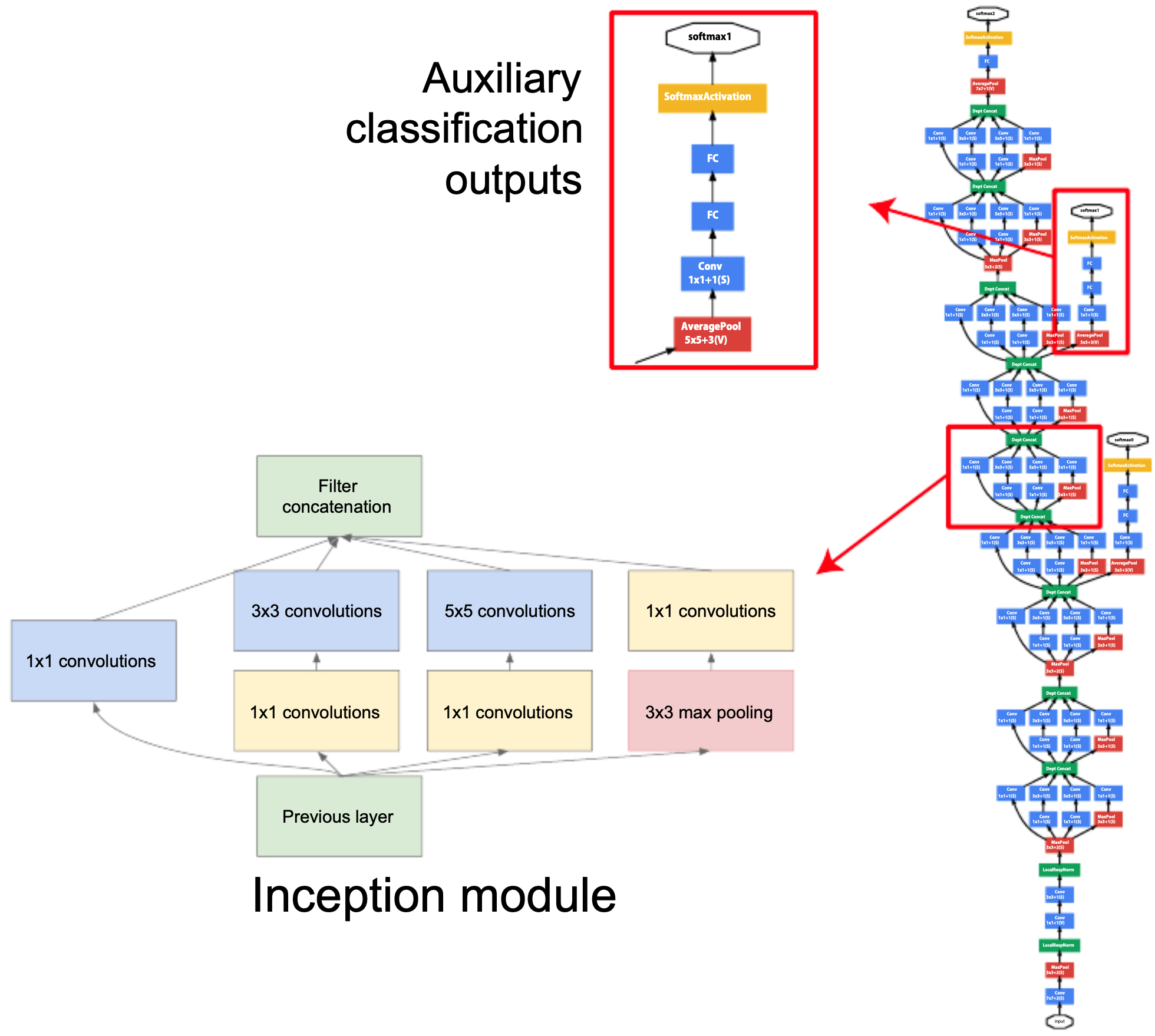
Auxiliary Classifiers

• Training very deep networks often suffers from vanishing gradients. To mitigate this, GoogLeNet introduced auxiliary classifiers attached to intermediate layers:

  • These small classifiers made predictions during training.
  • Their outputs were not used at test time but contributed to the loss during training, improving gradient flow and acting as a regularizer.

• This idea foreshadowed modern deep supervision strategies used in architectures like transformers.

Overall Architecture

• GoogLeNet was 22 layers deep, yet used only ~4M parameters (compared to VGG’s 138M). This was achieved by:

  • Eliminating fully connected layers (replaced with global average pooling).
  • Using inception modules with bottleneck layers.
  • Auxiliary classifiers for gradient stability.

• The following figure shows that the architecture of GoogLeNet, which consists of stacked inception modules with two auxiliary classification outputs.

Historical Impact

1. Shift in design philosophy: GoogLeNet showed that depth could be combined with architectural motifs (modules) rather than blindly stacking convolutional layers.
2. Efficiency: At ~15× fewer parameters than AlexNet, GoogLeNet enabled high performance on limited compute.
3. Scalability: The inception idea was extended into Inception-v3, Inception-v4, and Inception-ResNet, bridging CNNs with residual learning.

• GoogLeNet established a new paradigm: networks could be deep, wide, and computationally efficient.

ResNet

• The Residual Network (ResNet), introduced by He et al. (He et al., 2016), was a milestone in deep learning. It won the ILSVRC 2015 classification challenge with a top-5 error rate of 3.57%, surpassing the estimated human-level error rate of ~5% (Russakovsky et al., 2015). Beyond ImageNet, ResNet swept nearly every major vision benchmark that year, dominating detection, localization, and segmentation tasks.

The Degradation Problem

• Before ResNet, researchers attempted to improve accuracy by simply stacking more layers. Surprisingly, this often increased training error, not just test error. This was not due to overfitting but rather an optimization failure — deeper networks were harder to train effectively.

• The following figure illustrates that by simply stacking more layers onto a neural network, the authors of ResNet showed that the performance of the network will actually be worse.

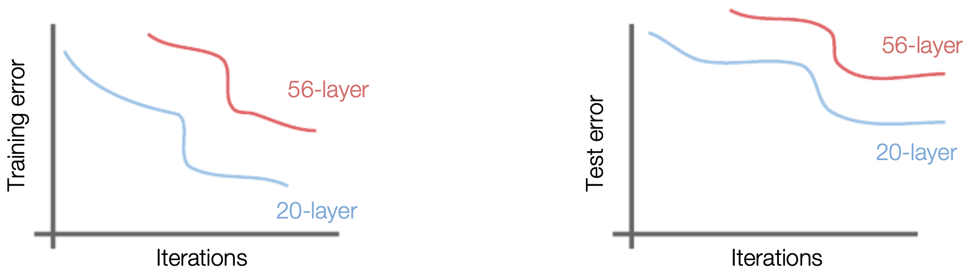
• This phenomenon, called the degradation problem, suggested that additional layers should have been able to learn at least as well as shallower ones — but in practice, optimization failed.

Core Idea: Residual Learning

• ResNet introduced skip connections (residual connections) to address this.

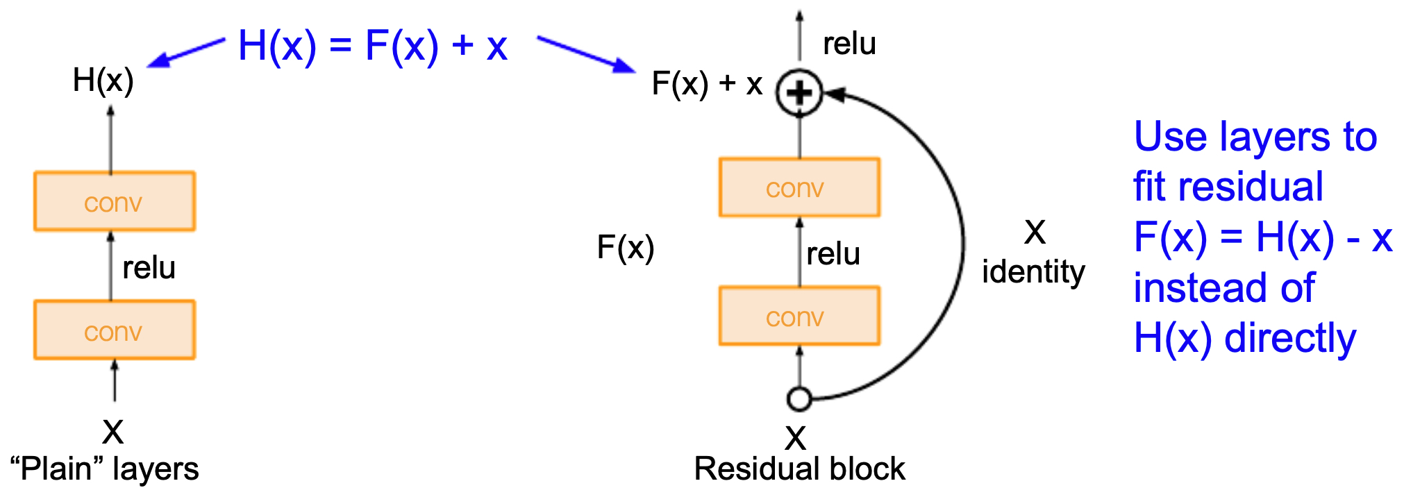
• A standard block learns a mapping \(H(x)\).
• ResNet reformulates this as learning a residual function:

• so that

• The input \(x\) is directly added to the block’s output, creating a shortcut.

• This makes it easier for the optimizer to approximate the identity mapping (when extra layers are unnecessary), stabilizing training even in very deep networks.

The Residual Block

• A basic residual block consists of two or three convolutional layers (each with BatchNorm and ReLU), plus the skip connection:

• If input and output dimensions match: skip is an identity mapping.

• If dimensions differ (e.g., downsampling), a \(1 \times 1\) convolution is used to align them.

• The following figure presents “plain” v/s residual blocks, with the skip connection bypassing convolutional layers.

• For networks deeper than 50 layers, ResNet introduced bottleneck blocks:

  • A \(1 \times 1\) convolution reduces dimensionality.
  • A \(3 \times 3\) convolution processes features.
  • Another \(1 \times 1\) convolution restores dimensionality.

• This reduced computation while maintaining expressivity.

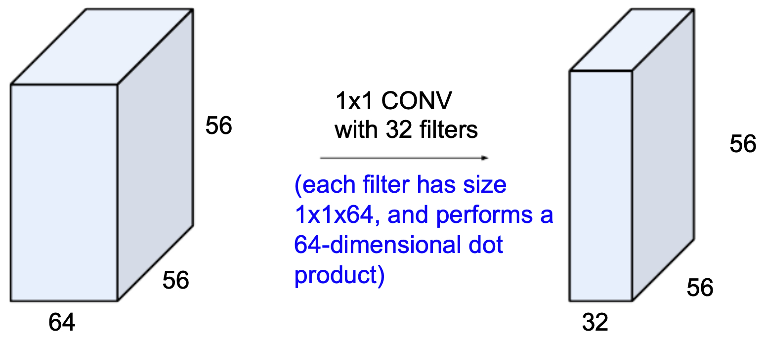
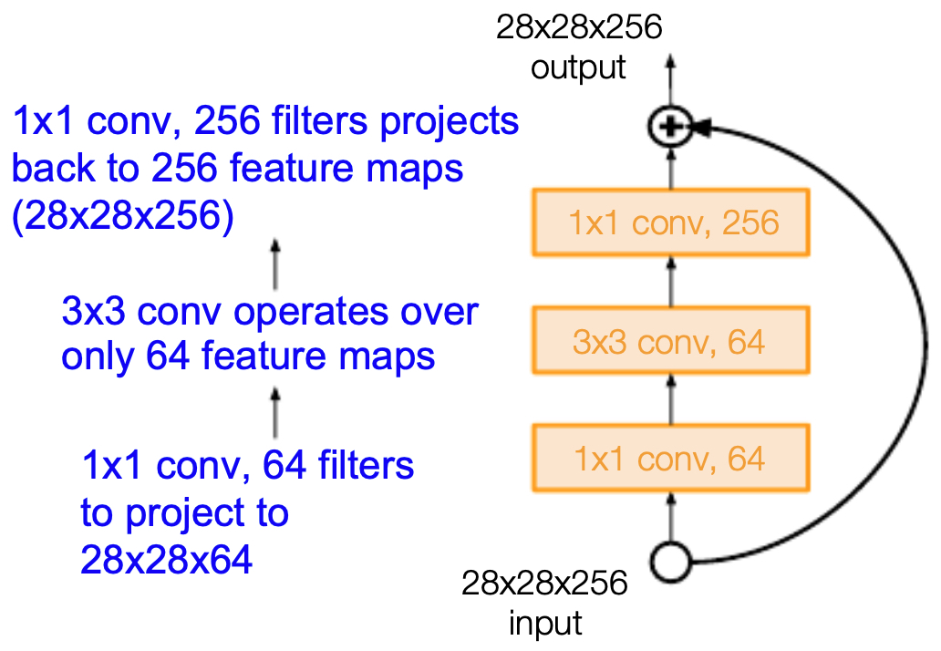
• The following figure shows bottleneck residual block: efficiency through \(1 \times 1\) convolutions by reducing dimensionality. The example below shows that applying a \(1 \times 1\) convolution with 32 filters to a \(56 \times 56 \times 64\) input produces a \(56 \times 56 \times 32\) output.

Training and Optimization

• ResNet’s success was not only architectural but also methodological. The authors employed:

  • Initialization: Xavier initialization for stable gradient flow.
  • Batch Normalization after each convolution.
  • Optimizer: SGD with momentum (0.9).
  • Learning rate schedule: initial 0.1, reduced by factor 10 at validation plateaus.
  • Batch size: 256.
  • Weight decay: \(10^{-5}\).

• These choices, coupled with residual learning, allowed networks as deep as 152 layers to be trained successfully — previously unthinkable.

Full Architecture

• ResNet architectures were proposed in variants of 34, 50, 101, and 152 layers. The deeper models used bottlenecks for efficiency.

• The following figures shows the full ResNet architecture: stacks of residual blocks with increasing depth.

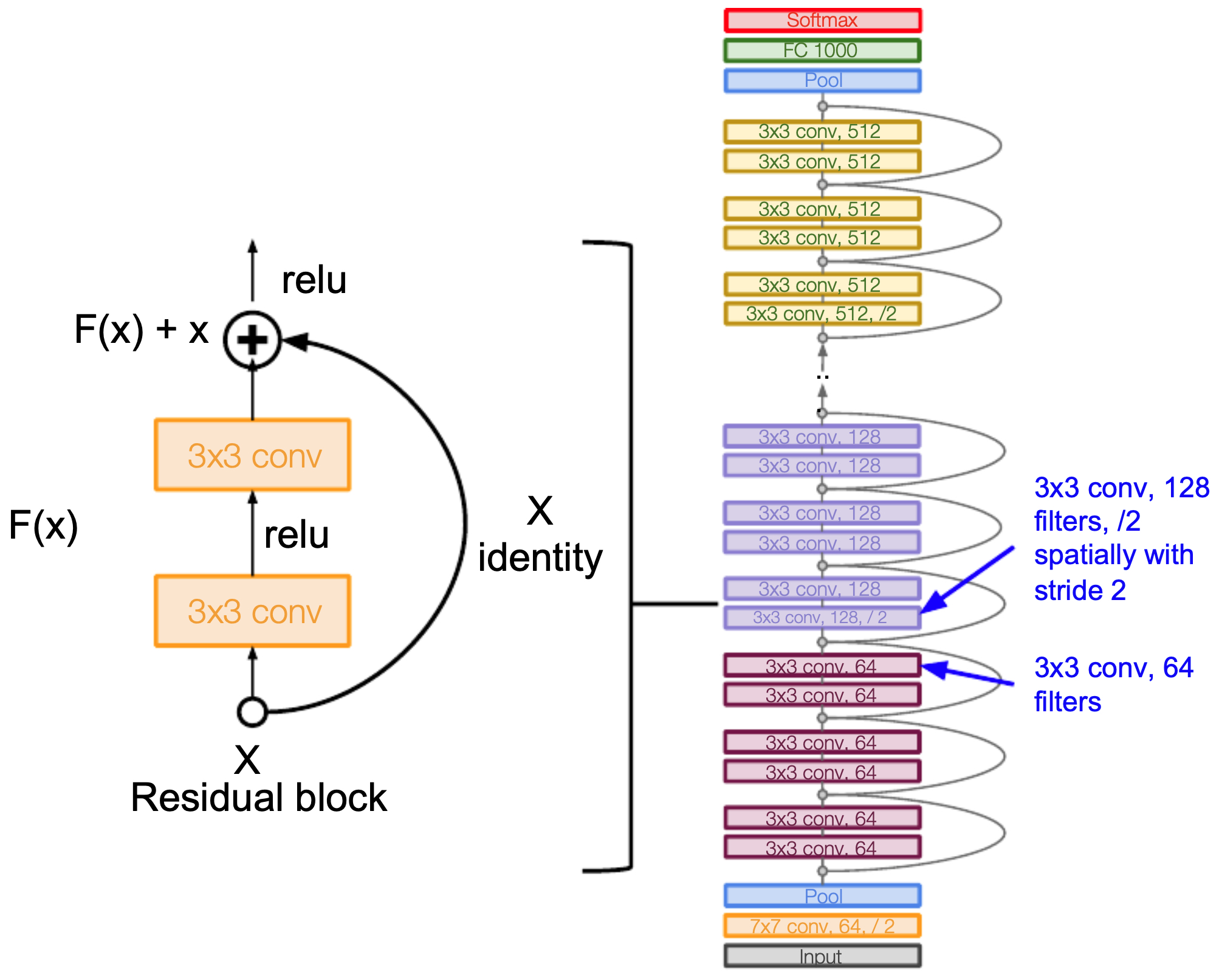
• For all of the models with ResNet models with over 50 layers, bottlenecking (the use of \(1 \times 1\) convolutions to change the depth of a network) was used to improve efficiency, as shown in the figure below.

Why Residuals Work

1. Improved gradient flow: Skip connections provide direct paths for gradients, reducing vanishing/exploding gradient issues.
2. Identity mappings: If deeper layers don’t help, residual blocks can learn \(F(x) = 0\), reverting to identity.
3. Ensemble-like behavior: ResNet behaves like an ensemble of shallower networks, where some paths bypass many layers.

Historical Impact

• ResNet revolutionized neural network design:

  • It made ultra-deep networks trainable, paving the way for 100+ and even 1000+ layer models.
  • It inspired architectures such as DenseNet, Inception-ResNet, and even influenced transformers (e.g., skip connections in BERT and Vision Transformers).
  • Beyond ImageNet, ResNet variants became default backbones in object detection (Faster R-CNN, Mask R-CNN), segmentation, and transfer learning.

• ResNet marked a paradigm shift: depth with skip connections, rather than plain stacking, became the new normal in deep learning.

DenseNet

• The Densely Connected Convolutional Network (DenseNet), introduced by Huang et al. (Huang et al., 2017), extended ResNet’s philosophy of skip connections. While ResNet introduced shortcuts between blocks, DenseNet pushed this further: every layer is directly connected to every other layer within a dense block.

• This design fundamentally rethought information flow in CNNs, enabling highly parameter-efficient, deeply connected models.

Core Contributions

1. Dense Connectivity Pattern

   • In a dense block with \(L\) layers, the \(l^{th}\) layer receives as input the feature maps of all preceding layers:

     \[x_l = H_l([x_0, x_1, \dots, x_{l-1}])\]
     • where \([ \cdot ]\) denotes concatenation and \(H_l\) is a composite operation (BatchNorm \(\rightarrow\) ReLU \(\rightarrow\) Convolution).

   • This design ensures maximum information flow between layers.

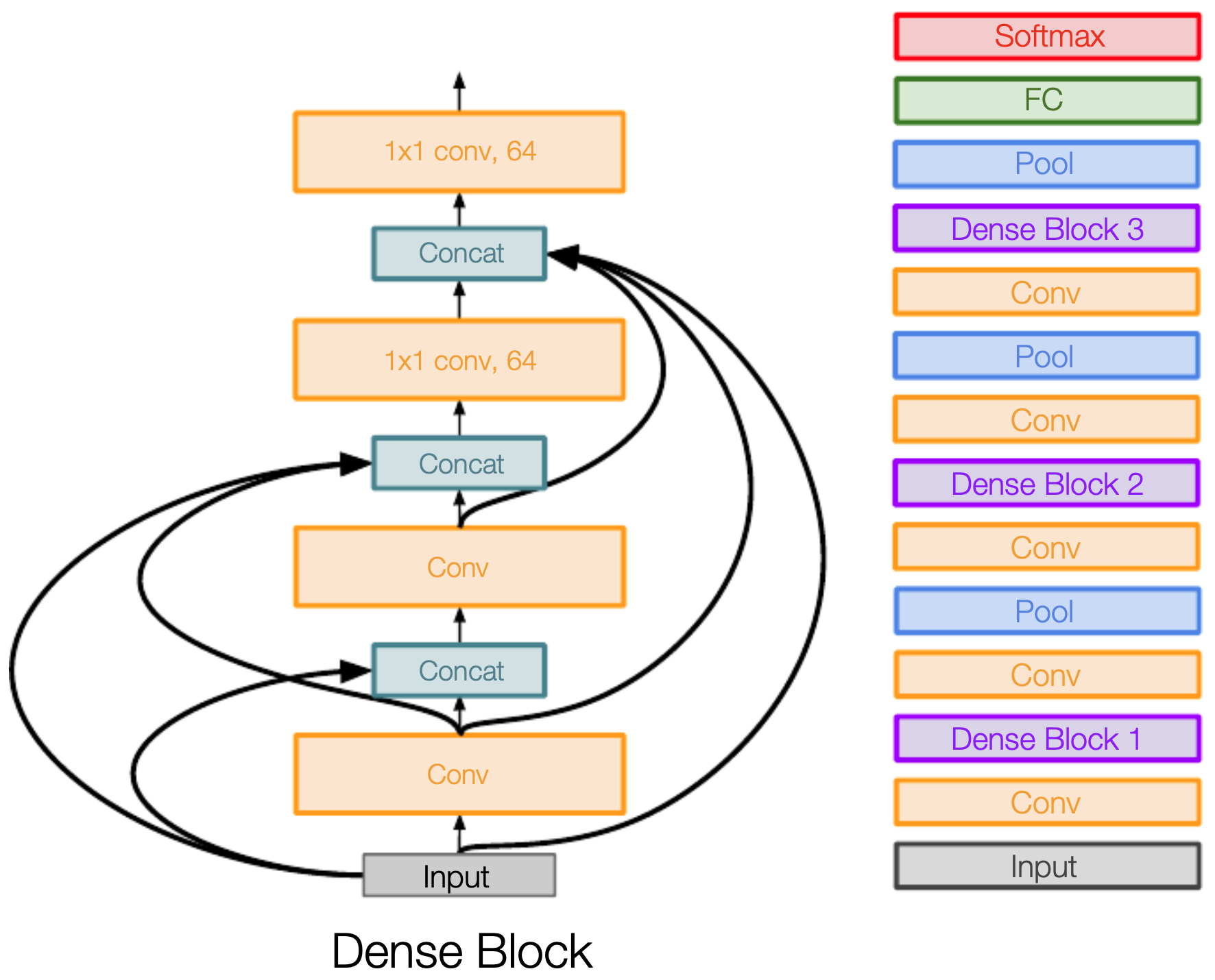
   • The following figure shows the DenseNet architecture. Each layer receives inputs from all previous layers (i.e., dense blocks concatenate all of the previous inputs into the input in later layers), leading to a web of connections within each dense block.

   

2. Feature Reuse

   • Instead of relearning redundant features, DenseNet promotes reuse of earlier representations.
   • Low-level features (edges, textures) are accessible to deeper layers without being re-extracted.

3. Mitigating Vanishing Gradients

   • Similar to ResNet, DenseNet strengthens gradient flow, but even more aggressively.
   • Direct connections ensure shallow layers receive supervisory signals during backpropagation.

4. Parameter Efficiency

   • Each layer only contributes a small number of new feature maps (the growth rate \(k\)).
   • Because features are reused, DenseNet requires fewer parameters than ResNet while maintaining high accuracy.

Architecture

• DenseNet is composed of two main components:

  • Dense Blocks: Sequences of densely connected layers.
  • Transition Layers: Between dense blocks, transition layers use \(1 \times 1\) convolutions and pooling to reduce feature-map sizes and prevent uncontrolled growth.

• The concatenation mechanism means that feature map dimensionality grows linearly with depth inside each block. Transition layers keep this growth tractable.

Impact

• DenseNet demonstrated that:

  1. Connectivity can matter more than depth. Instead of pushing to hundreds of layers, smarter connectivity patterns yielded superior performance.
  2. Efficiency and performance are not mutually exclusive. DenseNet achieved state-of-the-art results with fewer FLOPs and parameters compared to ResNet.
  3. Transfer learning strength. DenseNet became a widely used backbone in medical imaging and other fields where parameter efficiency was essential.

Historical Position

• ResNet (2015): Skip connections across blocks solved degradation.

• DenseNet (2017): Skip connections across all layers enabled maximal feature reuse.

• Together, they shifted CNN design toward connectivity-driven architectures rather than blind depth escalation.

Additional Architectures

• Beyond AlexNet, VGG, GoogLeNet, ResNet, and DenseNet, researchers proposed several innovative CNN variants between 2013 and 2017. These architectures explored new motifs, connectivity patterns, and training strategies, often addressing specific weaknesses of earlier designs.

Network in Network (NiN)

• Introduced by Lin et al. (Lin et al., 2013), NiN replaced traditional convolutional layers with micro multilayer perceptrons (MLPs) applied in a sliding-window fashion.

• The key idea was to use 1×1 convolutions not just for dimensionality reduction, but as learnable nonlinear projections.
• This allowed the network to model more complex functions while preserving spatial information.

• NiN set the stage for later architectures like GoogLeNet and ResNet, where 1×1 convolutions became fundamental building blocks (bottlenecks).

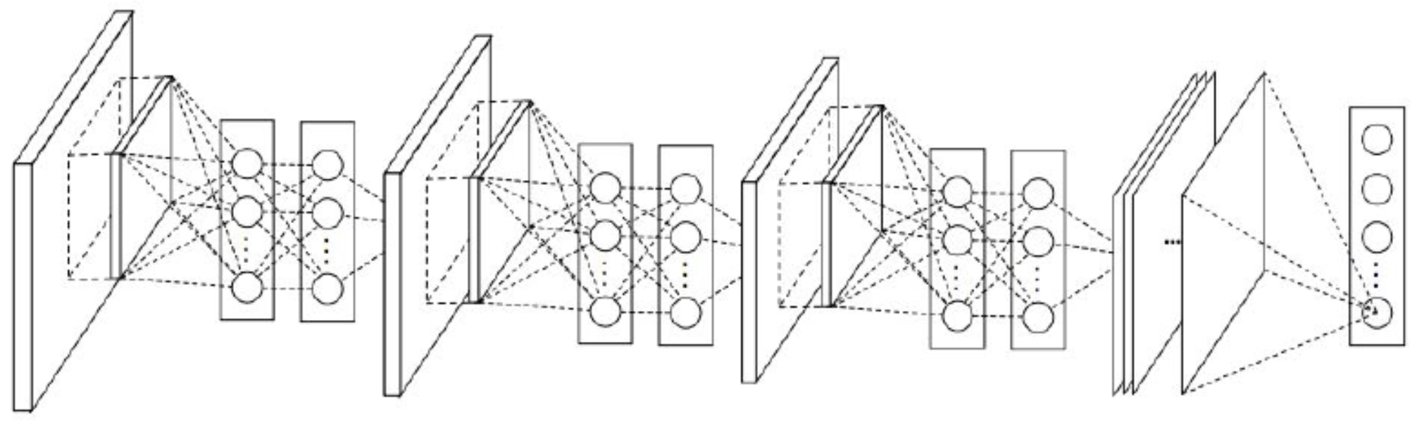
• The following figure shows the NiN architecture, where the fully-connected layers in the image represent the 1 1 convolution operations.

Wide ResNet

• Proposed by Zagoruyko and Komodakis, 2016, Wide ResNet’s premise is based on the fact that depth is not the only factor in ResNet’s success. Instead, they hypothesized that the residual block structure itself was more important than sheer layer count.

• Wide ResNet (WRN) increased the width (number of channels) of residual blocks while reducing depth.
• This improved parameter efficiency: fewer sequential layers, but more expressive filters per layer.

• WRNs achieved competitive or superior accuracy compared to 152-layer ResNets, while being easier to train and faster to run (better parallelization).

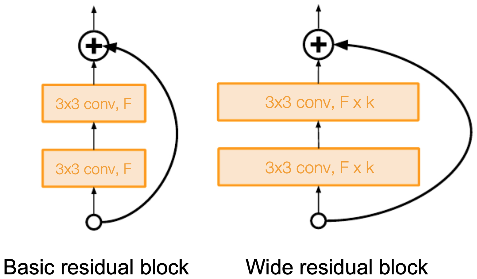
• The following figure shows Wide ResNet’s improved residual block design: fewer layers but wider channels.

ResNeXt

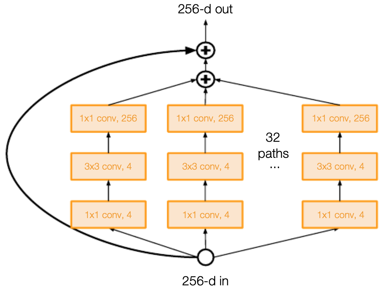
• Proposed by Xie et al., 2017, ResNeXt extended ResNet by adding a new dimension: cardinality, or the number of parallel paths in a block.

• Each ResNeXt block is a split-transform-merge structure: input features are split into parallel groups, each processed by its own transformation, and then aggregated.
• This design is conceptually similar to Inception modules but with a more homogeneous, scalable design.

• Empirically, increasing cardinality proved more effective than simply increasing depth or width.

• The following figure illustrates that adding cardinality to ResNet was the main contribution of ResNeXt. The ResNeXt block involved parallel paths (cardinality) combined within the residual framework.

Stochastic Depth

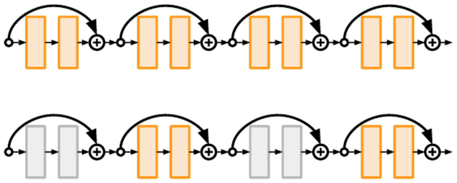
• Proposed by Huang et al., 2016, stochastic depth introduced a regularization method for very deep ResNets.

• During training, a random subset of residual blocks is skipped in each forward pass.
• This is analogous to dropout, but applied at the layer level rather than neuron level.
• At test time, the full network is used.

• Benefits:

  • Reduced training time (shorter expected path length).
  • Implicit ensemble of shallower subnetworks.
  • Improved generalization.
• The following figure illustrates that the original ResNet kept all the residual blocks activated during the training phase (top) while ResNet with stochastic depth turns off a random sample of residual blocks during each training pass (bottom).

FractalNet

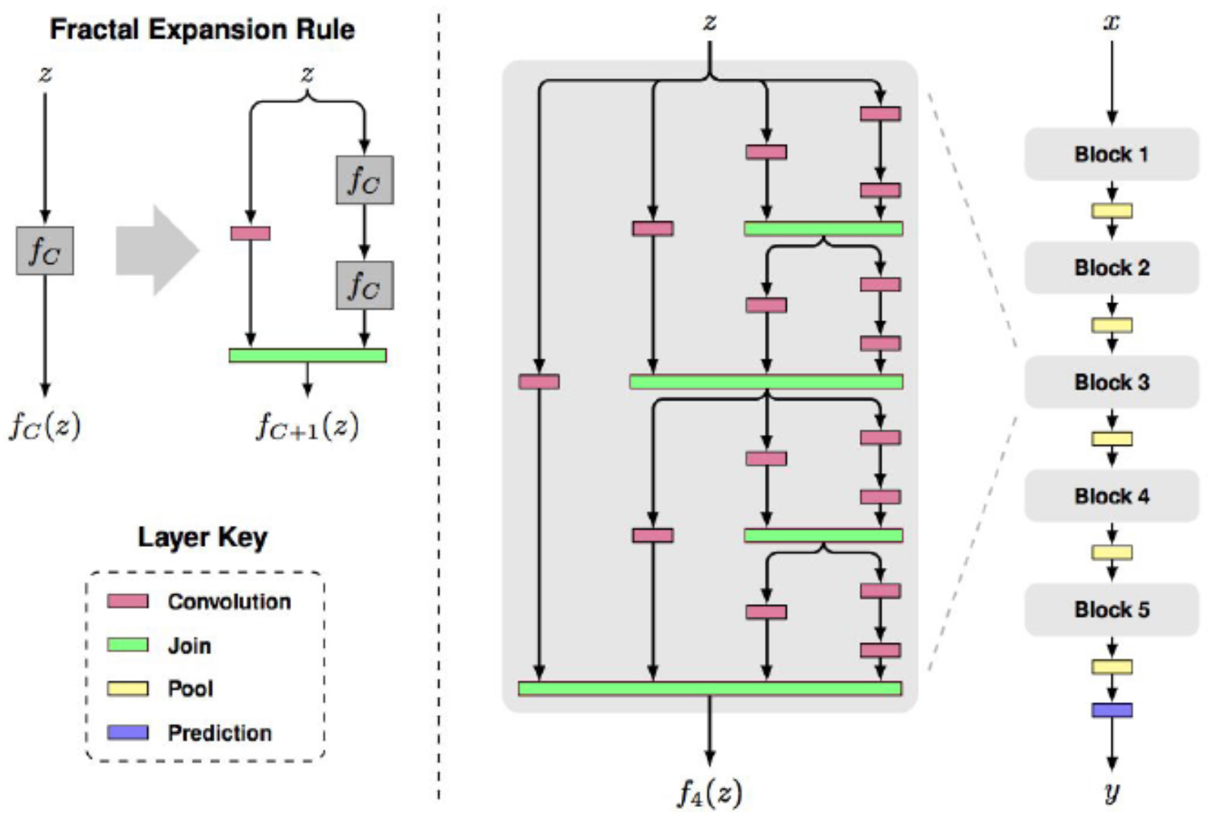
• Proposed by Larsson et al., 2016, FractalNet emphasized self-similarity and path diversity rather than residual connections.

• The architecture consisted of nested, self-similar fractal patterns of convolutional layers.
• Information could flow through multiple parallel paths of varying depths.
• Like stochastic depth, random path dropping was used during training as a form of regularization.

• At test time, all paths were active, effectively ensembling shallow and deep representations.

• The following figure shows the FractalNet architecture: fractal expansion creates multiple deep and shallow paths.

SqueezeNet

• Proposed by Iandola et al., 2016, SqueezeNet sought to drastically reduce parameter count without sacrificing accuracy.

• Parameter efficiency: Achieved AlexNet-level accuracy with 50× fewer parameters.
• Model size: <0.5 MB (≈510× smaller than AlexNet).

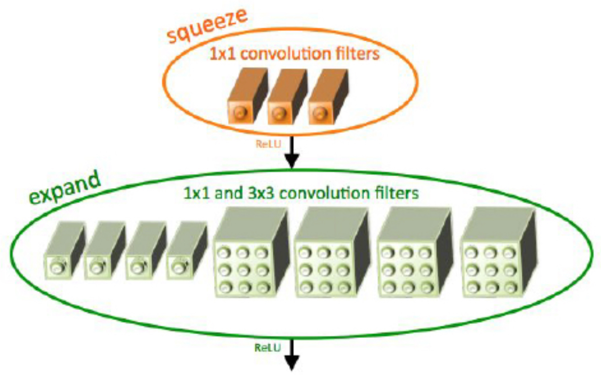
• Fire modules:

  • Squeeze stage: 1×1 convolutions reduce input channels.
  • Expand stage: Combination of 1×1 and 3×3 convolutions restores dimensionality.

• This design made SqueezeNet particularly attractive for mobile and embedded systems.

• The following figure shows Fire modules: compress with 1×1 convolutions, then expand with 1×1 and 3×3 filters.

Summary of Additional Contributions

• NiN: Introduced 1×1 convolutions as nonlinear feature projectors.
• Wide ResNet: Demonstrated that width can rival depth for efficiency and accuracy.
• ResNeXt: Added cardinality (parallel paths) as a new axis of scaling.
• Stochastic Depth: Improved training by randomly dropping entire blocks.
• FractalNet: Explored fractal-like, multi-path connectivity without residuals.

• SqueezeNet: Made CNNs deployable on constrained hardware with extreme parameter efficiency.

• Together, these architectures highlighted that depth is not the only frontier — efficiency, width, cardinality, and connectivity diversity all contribute to CNN advancement.

The Future of CNNs: Efficiency and Beyond

• After the breakthroughs of ResNet (2015) and DenseNet (2017), research in CNNs shifted toward efficiency and deployability. While ultra-deep networks achieved record-breaking accuracies, their computational and memory demands made them impractical for many real-world applications, such as mobile devices, embedded systems, and real-time video.

Historical Trends

• The trajectory of CNN performance versus computational cost can be visualized in benchmark comparisons:

• The following figure provides a historical overview of the top-1 percent accuracy of each network based on the number of operations. The size of the circle denotes the amount of memeory that the network uses.

• AlexNet (2012): Dramatic accuracy improvement, but parameter-heavy.
• VGG (2014): Deep (16–19 layers), ~138M parameters, high memory and compute cost.
• GoogLeNet (2014): Achieved higher accuracy with 15× fewer parameters than AlexNet.
• ResNet (2015): Ultra-deep (152 layers) yet trainable, with residual learning.
• DenseNet (2017): Fewer parameters, more efficient connectivity.

A complementary perspective compares forward pass times and power usage, illustrating deployment concerns:

• The following figure shows forward propagation times (in ms) for popular networks, along with their power usage.

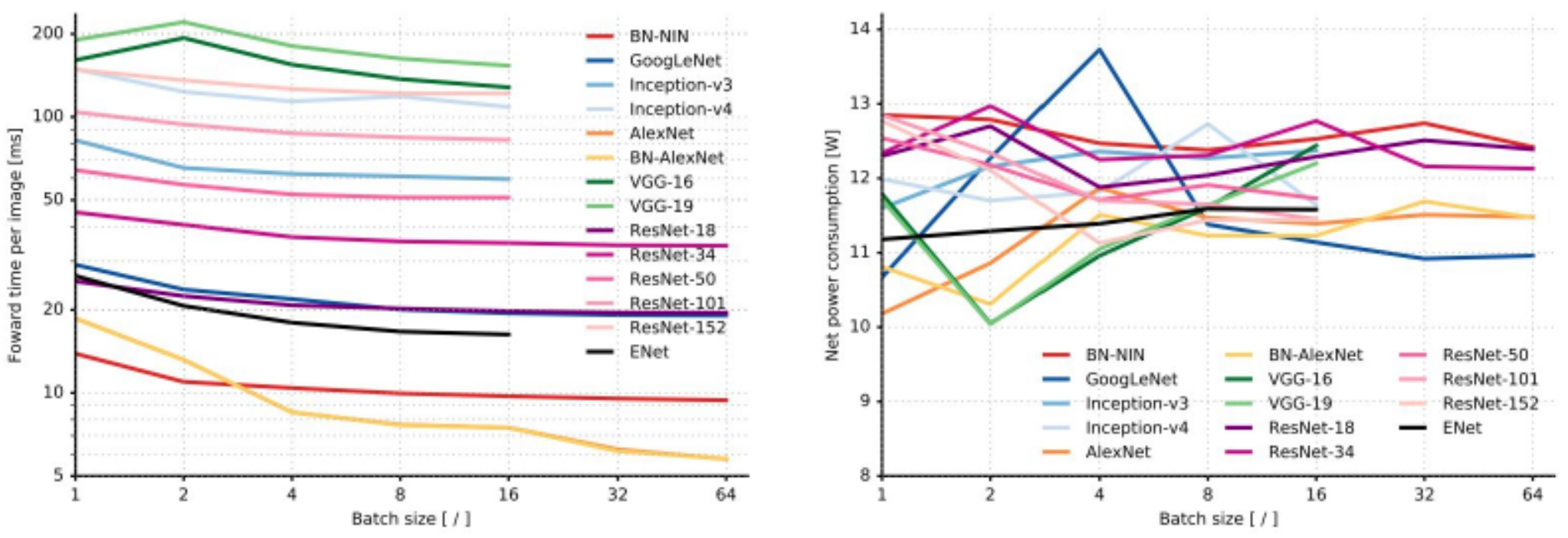
• These comparisons, as analyzed in Canziani et al., 2016, showed that accuracy gains often came at steep computational costs.

Efficient Architectures

• To balance accuracy with deployment feasibility, several efficient CNN architectures were proposed:

1. SqueezeNet (Iandola et al., 2016)

   • Achieved AlexNet-level accuracy with 50× fewer parameters.
   • Introduced fire modules: a squeeze stage (1×1 filters) followed by an expand stage (1×1 and 3×3 filters).
   • Produced a model under 0.5 MB — ~510× smaller than AlexNet.

   (Fire modules: 1×1 squeeze followed by 1×1 and 3×3 expand convolutions.)

2. MobileNet (Howard et al., 2017)

   • Introduced depthwise separable convolutions:

     • Depthwise convolution: one filter per channel.
     • Pointwise convolution (1×1): combines channel outputs.
   • Reduced computation by ~9× with minor accuracy tradeoffs.
   • Widely adopted in mobile vision applications (e.g., Google Lens).

3. ShuffleNet (Zhang et al., 2018)

   • Used group convolutions and channel shuffling to enable cross-channel information exchange.
   • Designed for high efficiency on low-power devices.

• These networks marked CNNs’ shift from accuracy-at-all-costs to practical, deployment-ready models.

Hybrid Architectures: Inception-ResNet

• Researchers also began combining architectural motifs:

  • Inception modules: multi-scale feature extraction.
  • Residual connections: stabilized training of deep networks.

• Inception-ResNet (Szegedy et al., 2017) fused these two, outperforming both standalone designs by combining feature diversity and gradient stability.

Looking Ahead

• CNN research increasingly emphasizes scalability, efficiency, and hybridization. Several emerging directions include:

  • Neural Architecture Search (NAS): Automated methods to discover architectures optimized for accuracy vs. compute tradeoffs (Zoph and Le, 2017).
  • Dynamic inference: Models that adapt computation based on input complexity.
  • Hybrid models: Integration of CNNs with transformers for spatiotemporal modeling (e.g., Vision Transformers, ViTs).
  • Domain-specific design: Custom efficiency for edge AI, AR/VR, and medical imaging.

Legacy

• The trajectory from AlexNet \(\rightarrow\) ZFNet \(\rightarrow\) VGG \(\rightarrow\) GoogLeNet \(\rightarrow\) ResNet \(\rightarrow\) DenseNet reflects an evolution in priorities:

  • From proving CNNs work (AlexNet).
  • To interpretability (ZFNet).
  • To depth and simplicity (VGG).
  • To modular efficiency (GoogLeNet).
  • To ultra-deep optimization (ResNet).
  • To connectivity-driven efficiency (DenseNet).

• This lineage continues to inspire the next generation of architectures, balancing accuracy, interpretability, and deployability in ever more resource-constrained environments.

Citation

If you found our work useful, please cite it as:

@article{Chadha2020CNNArchitectures,
  title   = {CNN Architectures},
  author  = {Chadha, Aman},
  journal = {Distilled Notes for Stanford CS231n: Convolutional Neural Networks for Visual Recognition},
  yewith    = {2020},
  note    = {\url{https://aman.ai}}
}