CS231n • Convolutional Neural Networks
- Background: The History of Neural Networks
- Convolutional Neural Networks
- Spatial Dimensions
- Padding and Pooling Layers
- Advanced CNN Architectures
- Technical Building Blocks of CNNs
- Applications of CNNs
- Future Directions and Challenges
- Citation
Background: The History of Neural Networks
- The evolution of neural networks is a story of alternating optimism and skepticism. Neural networks have gone through multiple waves of enthusiasm, setbacks, and rediscovery. Today’s Convolutional Neural Networks (CNNs) are built upon decades of research that shaped the way we think about artificial intelligence and learning systems.
Early Foundations: The Perceptron
- In 1958, Frank Rosenblatt introduced the perceptron algorithm (Rosenblatt, 1958), an early computational model inspired by biological neurons. The perceptron was designed primarily for image recognition tasks, such as identifying letters of the alphabet. In its original demonstration, a camera produced \(20 \times 20\) pixel images, which were classified by computing a linear test function:
-
At the time, the backpropagation algorithm had not yet been invented, so perceptron training used heuristic methods to approximate the gradient direction.
-
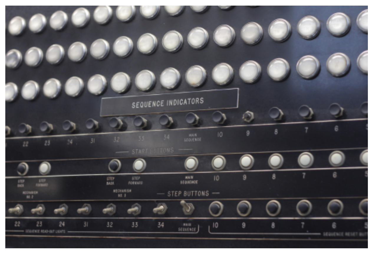
The following figure presents the Harvard Mark I Computer used for early calculations with the perceptron algorithm. This machine, one of the first electromechanical computers, symbolized the blend of pioneering hardware and emerging theories of artificial intelligence.
-
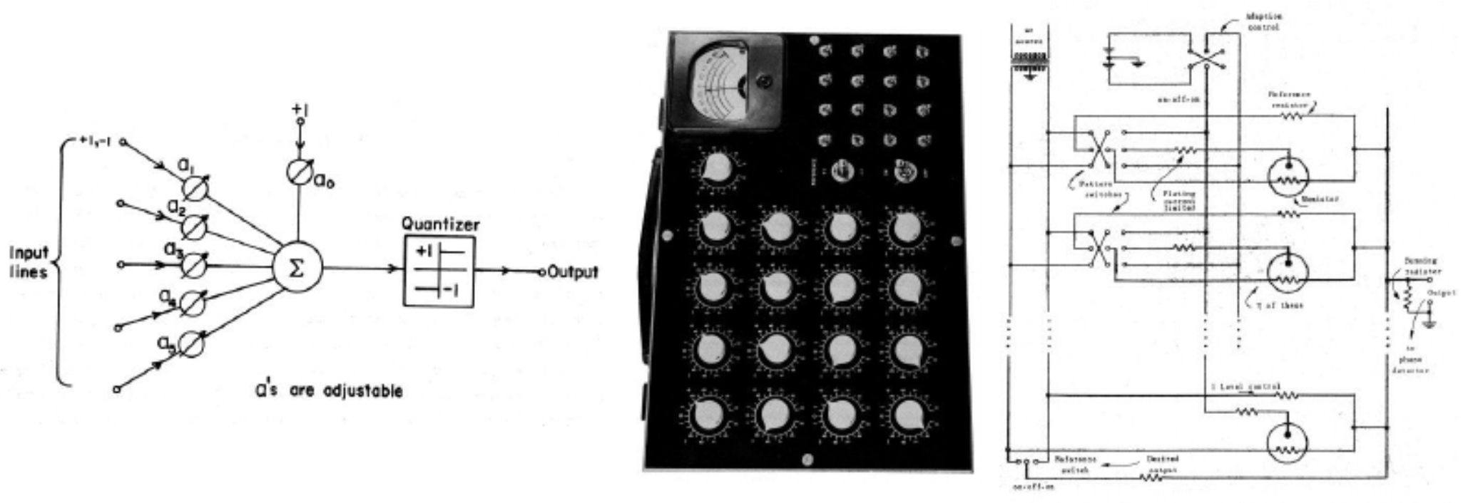
Just one year later, in 1959, Bernard Widrow and Marcian Hoff introduced Adaline (Adaptive Linear Neuron) and its extension, Madaline (Many Adalines) (Widrow & Hoff, 1960). These models stacked multiple linear units together, marking one of the first attempts to design layered networks. However, they still lacked an effective method for weight updates beyond heuristics.
-
The following figure shows images from the first known paper where researchers began to stack perceptrons together to form deeper networks. This work foreshadowed modern multilayer perceptrons.
The First AI Winter
-
Optimism around perceptrons diminished in the late 1960s. In their influential book Perceptrons (1969), Marvin Minsky and Seymour Papert demonstrated that single-layer perceptrons could not solve basic but critical non-linear tasks, such as the XOR problem. This revelation led to a decline in research funding and enthusiasm, ushering in the first AI winter.
-
Still, the seed had been planted: researchers imagined ways to extend simple perceptrons into multilayered networks.
-
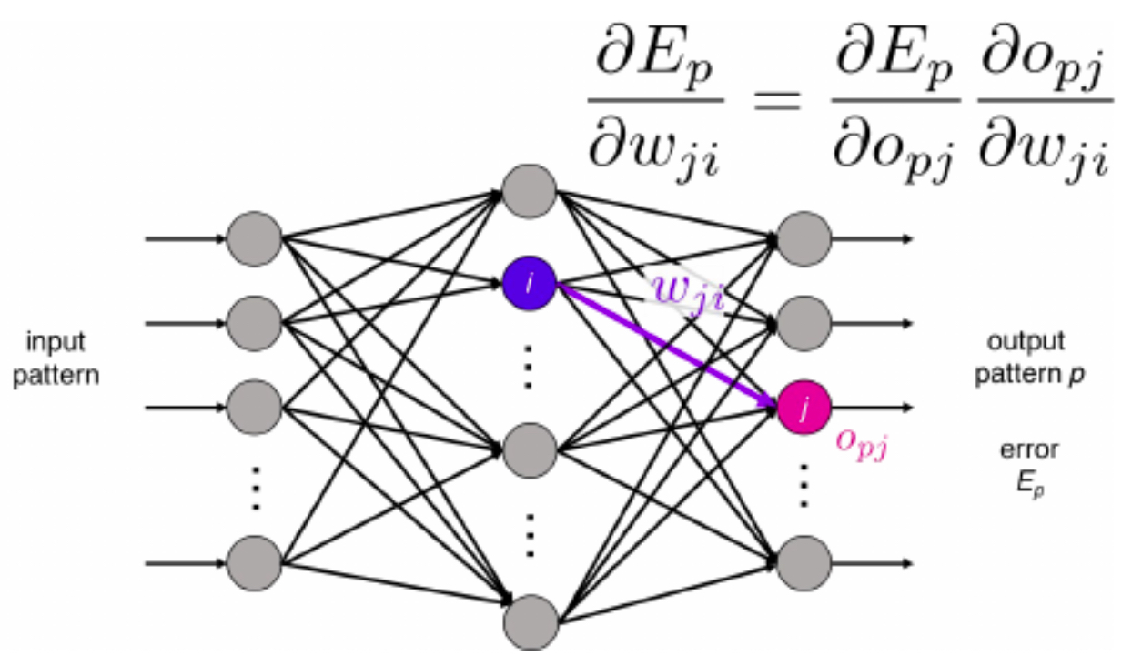
In 1986, David Rumelhart, Geoffrey Hinton, and Ronald Williams reintroduced backpropagation as a practical method to train multilayer perceptrons (Rumelhart et al., 1986). Their work sparked a revival of interest, as backpropagation allowed networks to learn complex mappings with many layers.
-
The following figure shows the recreation of Rumelhart et al. (1986), whose backpropagation framework became the foundation for all modern deep learning.
The Deep Learning Breakthrough
-
Despite the backpropagation revival, neural networks in the 1990s were still shallow and often underperformed compared to statistical machine learning methods such as support vector machines. Training deep networks remained unstable due to vanishing gradients.
-
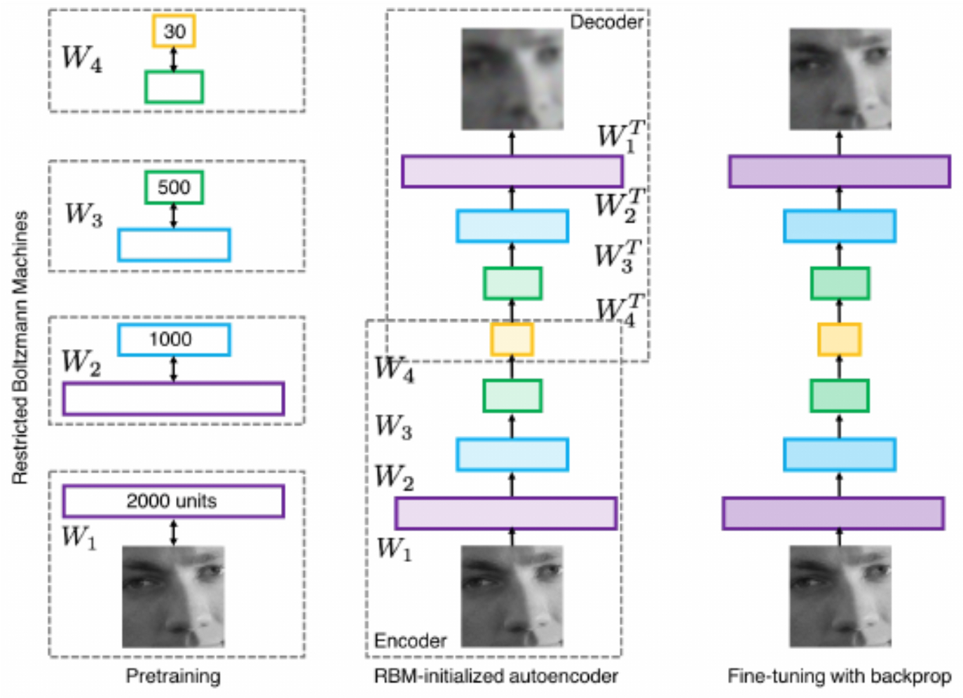
A turning point came in 2006, when Geoffrey Hinton and Ruslan Salakhutdinov demonstrated that deep belief networks could be trained layer by layer using Restricted Boltzmann Machines (Hinton & Salakhutdinov, 2006). Each layer was pretrained in an unsupervised fashion, then fine-tuned with supervised learning, overcoming previous training barriers.
-
The following figure summarizes the method of Hinton and Salakhutdinov. Their approach showed that deep models could be trained effectively, paving the way for the resurgence of neural networks.
CNNs in the Spotlight: AlexNet and ImageNet
-
The revival of neural networks coincided with two critical enablers: the advent of GPUs for large-scale training and the availability of massive labeled datasets like ImageNet (Deng et al., 2009).
-
In 2012, AlexNet—developed by Alex Krizhevsky, Ilya Sutskever, and Geoffrey Hinton—revolutionized computer vision (Krizhevsky et al., 2012). AlexNet was an eight-layer CNN that achieved unprecedented accuracy on the ImageNet Large Scale Visual Recognition Challenge (ILSVRC).
-
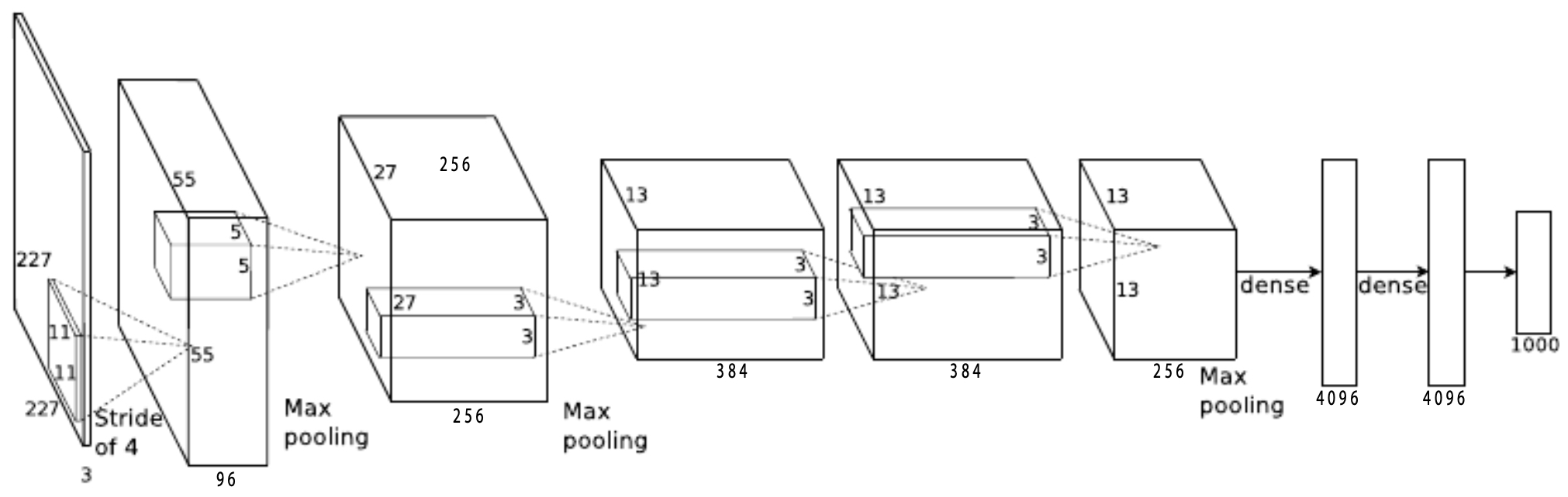
The following figure presents the AlexNet architecture. The input image of size \(224 \times 224\) passes through stacked convolutional and fully connected layers to produce a 1000-dimensional classification score.
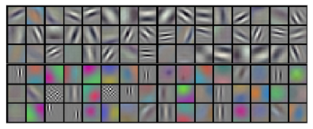
- The following figure depicts the filters learned in the first layer of AlexNet. These filters resemble edge detectors, color blobs, and texture patterns—revealing how CNNs learn low-level features similar to those in human vision.
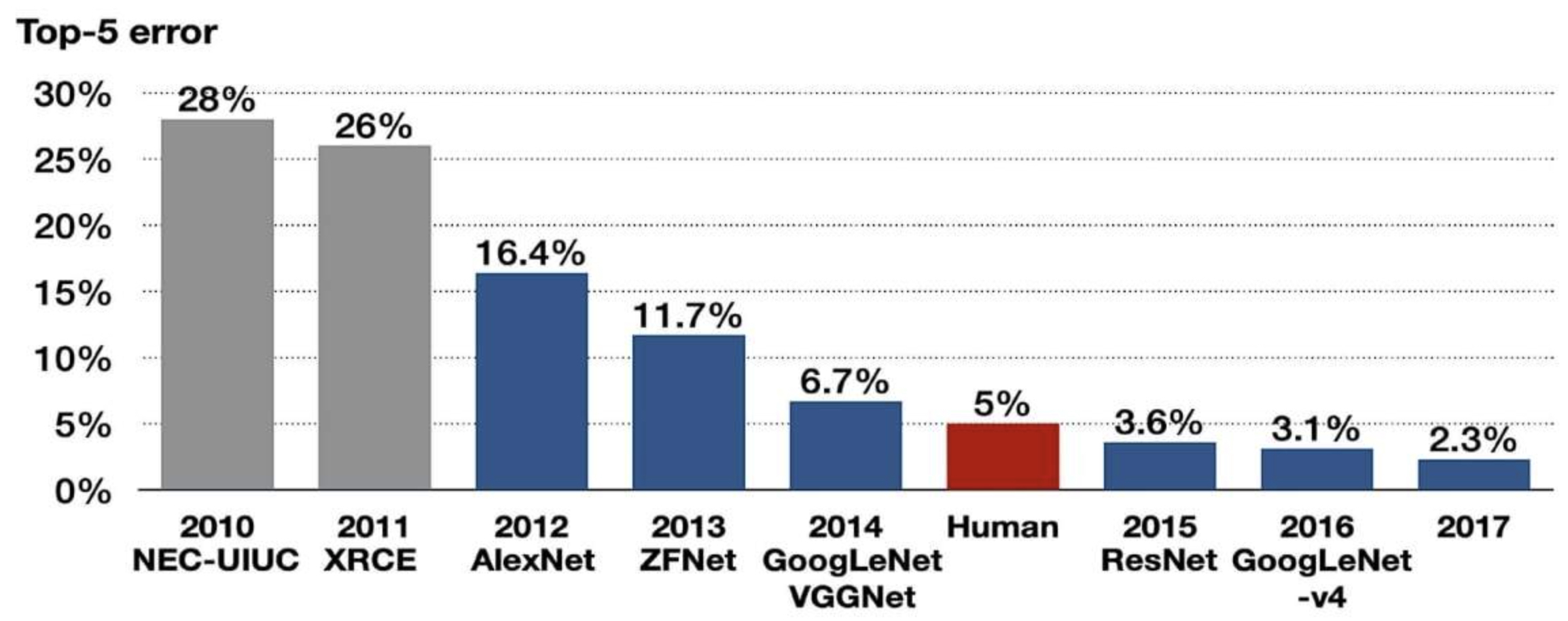
- The following figure shows the dramatic reduction in ImageNet classification error rates. AlexNet in 2012 cut the error rate from 28.2% to 15.3%, marking a watershed moment that launched the deep learning revolution.
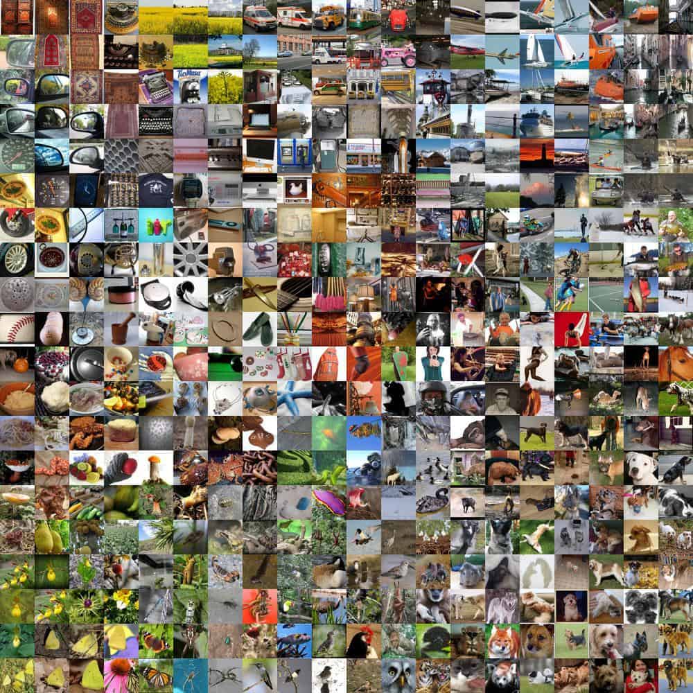
- The following figure presents a sample of the ImageNet dataset used to train AlexNet. The dataset’s scale and diversity across categories such as animals, vehicles, and objects enabled CNNs to generalize across real-world scenarios.
CNNs in Creativity and Beyond
-
Following AlexNet, CNNs rapidly expanded to applications beyond classification, including real-time detection, segmentation, pose estimation, self-driving cars, games, image captioning, and artistic style transfer (Gatys et al., 2015).
-
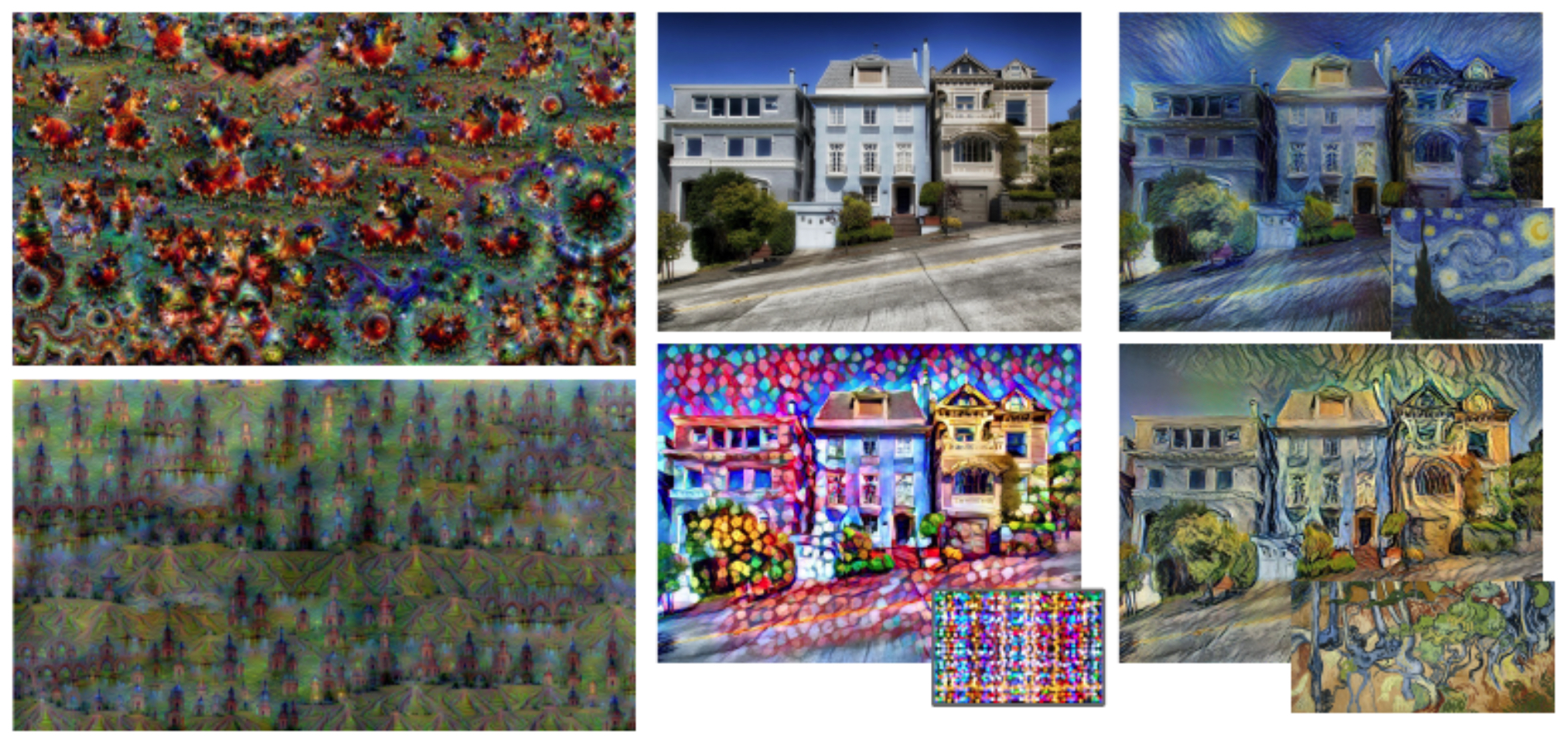
The following figure presents a few examples of CNN-driven generative art. These images highlight how CNNs capture both structural content and stylistic texture, enabling creative applications at the intersection of vision and art.
Legacy of the CNN Revolution
-
By the mid-2010s, CNNs became the cornerstone of computer vision, replacing manual feature engineering with automated feature extraction. Their hierarchical representation learning—edges and corners in shallow layers, objects and scenes in deep layers—set the stage for the deep learning revolution.
-
Modern AI applications in medical imaging, autonomous vehicles, and entertainment all trace their lineage back to the CNN breakthroughs of the 2010s.
Convolutional Neural Networks
- Convolutional Neural Networks (CNNs) are a class of deep learning models specifically designed to process structured grid-like data, such as images. Unlike traditional fully connected neural networks, which flatten an image into a single vector (discarding spatial relationships), CNNs preserve spatial structure and exploit local connectivity. This property makes them especially powerful for vision tasks.
Fully Connected Networks vs. Convolutional Networks
-
In a fully connected (dense) layer, every input pixel is connected to every neuron in the next layer. While expressive, this approach is inefficient for high-dimensional inputs such as images. For instance, a \(224 \times 224\) RGB image (common in ImageNet) has over 150,000 input values. Even a modest hidden layer connected to all pixels would yield millions of parameters—making training inefficient and prone to overfitting.
-
The following figure shows the structure of a fully connected neural network where a \(32 \times 32 \times 3\) image is flattened into a vector of 3072 values and passed through a dense weight matrix. Notice how spatial structure is lost.
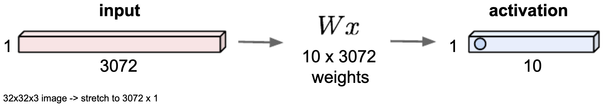
- CNNs address this inefficiency by introducing convolutional layers, which drastically reduce the number of parameters while retaining spatial hierarchies.
The Convolution Operation
-
At the heart of a CNN lies the convolution operation. Instead of connecting every pixel to every neuron, a CNN applies small filters (also called kernels or receptive fields) across localized regions of the image.
-
A filter is typically a small matrix of weights, such as \(3 \times 3\) or \(5 \times 5\), whose depth matches the input’s depth (e.g., depth = 3 for RGB images). As the filter slides across the image, it computes a dot product between its weights and local pixel values, producing a single scalar. Repeating this process across the entire image yields a feature map (or activation map).
-
The following figure illustrates a single step in convolution (a), where the filter overlaps a \(5 \times 5 \times 3\) region of the image and computes a dot product. Part (b) shows how the filter is systematically slid across the entire image to generate the activation map.
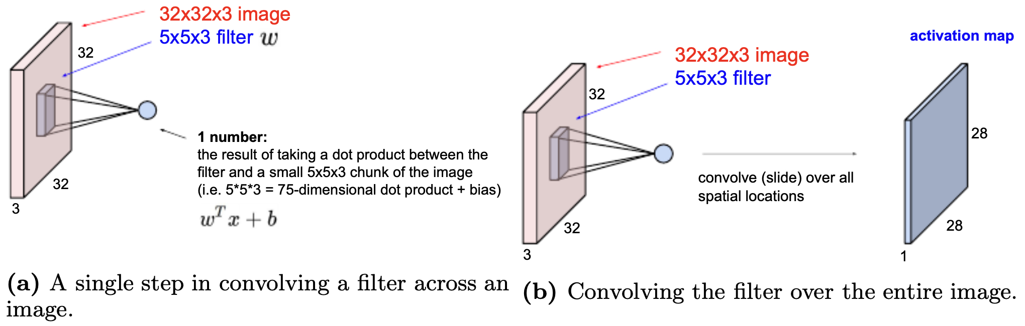
- This local connectivity ensures the network focuses on nearby patterns—edges, corners, or textures—which are later combined into higher-level concepts.
Activation Maps and Depth
-
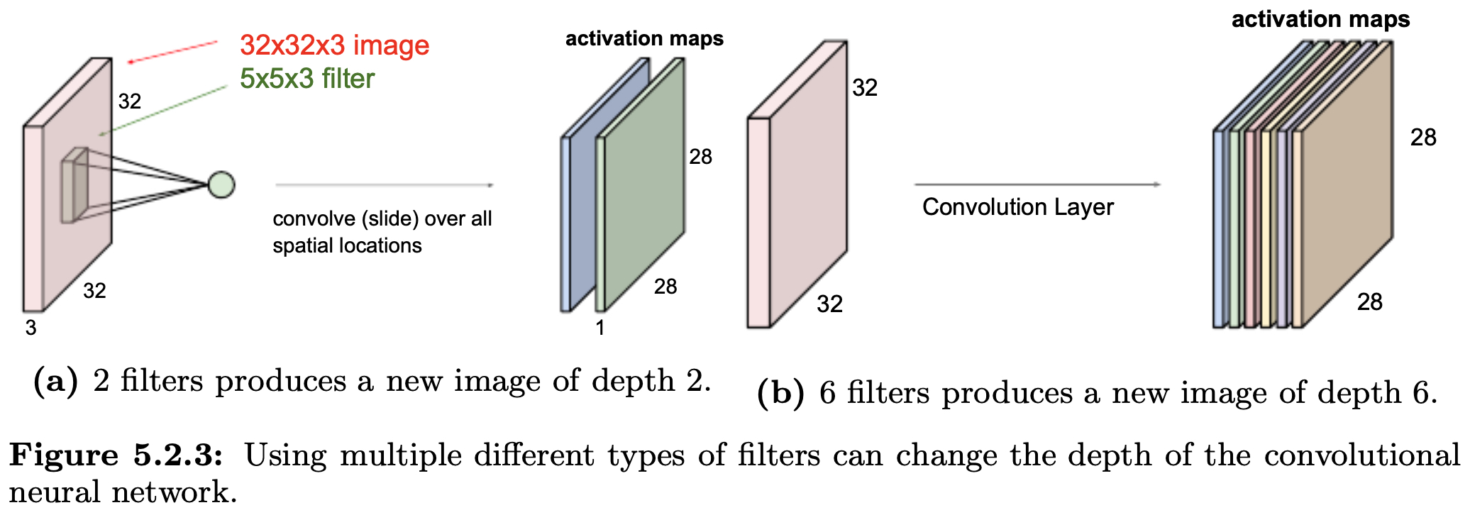
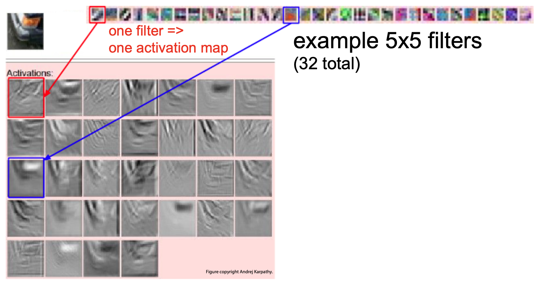
Each filter produces one activation map. Using multiple filters allows the network to detect multiple types of features simultaneously (e.g., vertical edges, diagonal lines, textures). These maps are stacked together to form the input for the next layer, increasing the depth of the representation.
-
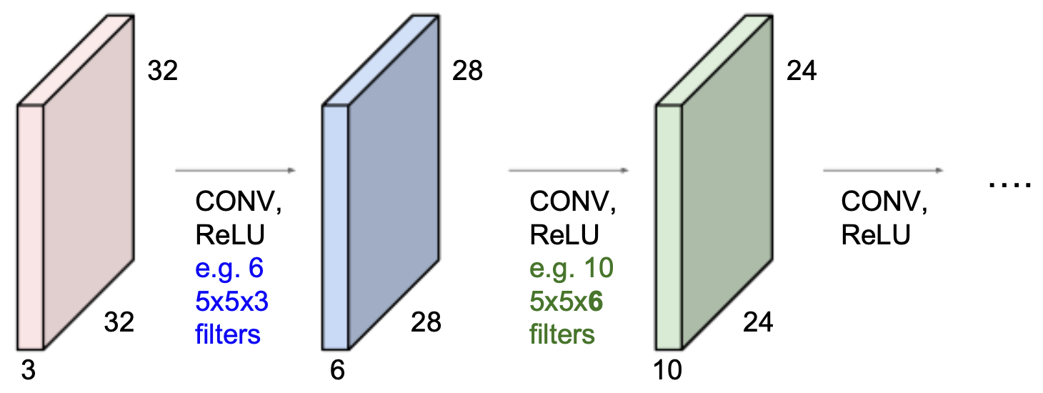
The following figure shows how multiple filters expand the depth of CNN outputs. With two filters, the depth of the output is 2; with six filters, the depth becomes 6. This depth expansion enables CNNs to capture a wide variety of patterns.
-
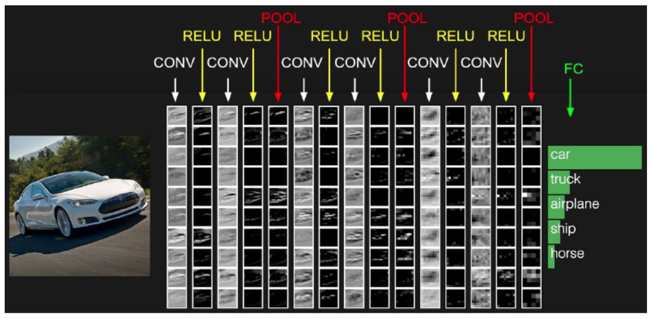
By stacking multiple convolutional layers, CNNs form a hierarchy of features. Each convolutional layer is followed by a nonlinearity function (commonly ReLU), allowing the network to learn complex, nonlinear mappings.
-
The following figure shows how CNNs are constructed by stacking convolutional layers in sequence, each followed by nonlinear activation functions. This design mirrors the hierarchical organization of the human visual cortex.
From Low-Level to High-Level Features
-
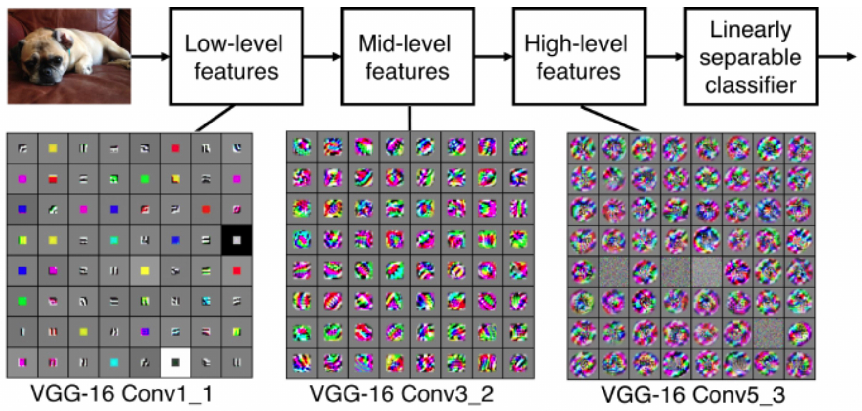
The power of CNNs lies in their ability to transition from low-level features (edges, lines, textures) to high-level abstractions (faces, objects, scenes) as network depth increases. This is reminiscent of Hubel and Wiesel’s discoveries in neuroscience, where early visual cortex neurons respond to edges and corners, while later neurons respond to complex patterns.
-
The following figure shows that earlier CNN layers learn filters for detecting edges and corners, while deeper layers capture semantic concepts such as objects and faces.
- The following figure shows example activation maps produced by filters. White pixels indicate strong positive activations, black pixels strong negative activations, and gray pixels neutral responses. These maps reveal which regions of the input most strongly match a filter’s learned feature.
- As we move deeper into the network, activation maps become increasingly abstract. The following figure shows activation maps across multiple layers of a CNN, illustrating the progression from low-level visual primitives to high-level structured representations.
Why CNNs Work So Well
-
CNNs achieve efficiency and accuracy through three core principles:
- Local Receptive Fields: Each filter is connected only to a small, localized region of the input, dramatically reducing the number of parameters.
- Shared Weights: The same filter is applied across the entire image, enabling feature detection regardless of spatial location and ensuring translation invariance.
- Hierarchical Feature Learning: Stacked convolutional layers progressively build from edges and textures to objects and categories, analogous to biological vision systems.
-
Together, these properties make CNNs scalable to large datasets and highly effective for complex vision tasks such as recognition, detection, and generation.
Spatial Dimensions
-
One of the most important considerations in CNN design is understanding how the output dimensions change as an image passes through convolutional layers. These dimensions depend on three factors:
- Input size (\(N \times N\)): the width and height of the input image.
- Filter size (\(F \times F\)): the spatial dimensions of the convolutional filter.
- Stride (\(S\)): the step size the filter moves across the input.
-
The general formula for computing the output size is:
- This assumes no padding and ensures that every step of the filter is valid (i.e., it fully overlaps with the input).
Example: \(7 \times 7\) Image with \(3 \times 3\) Filter
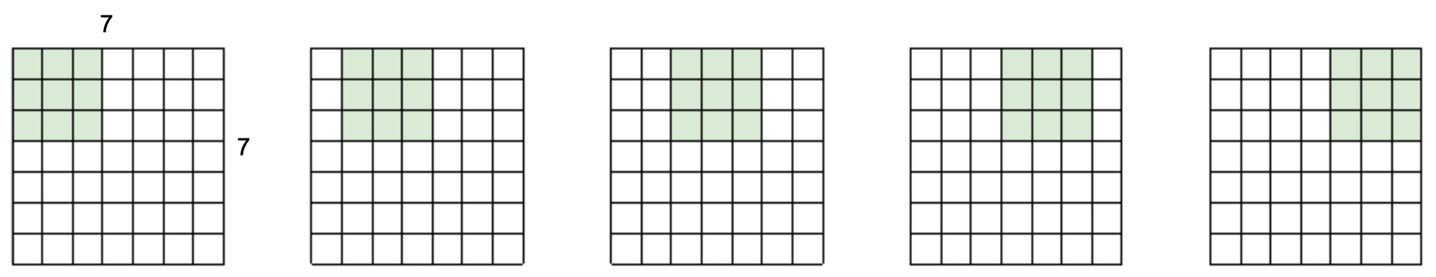
- Consider a \(7 \times 7\) input image convolved with a \(3 \times 3\) filter at stride 1:
-
This produces a \(5 \times 5\) output. Each entry corresponds to one valid position where the filter overlaps with the image.
-
The following figure shows how convolving a \(7 \times 7\) image with a \(3 \times 3\) filter produces a \(5 \times 5\) output. The highlighted operations depict horizontal convolutions; vertical convolutions follow the same principle.
Effect of Stride
-
The stride controls how far the filter shifts each time. A stride of 1 results in overlapping coverage, while larger strides reduce overlap and shrink the output size.
-
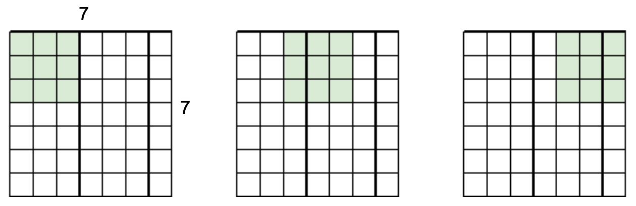
For example, with a \(7 \times 7\) image and a \(3 \times 3\) filter using stride 2:
-
This yields a \(3 \times 3\) output, compressing the representation by skipping intermediate positions.
-
The following figure shows how a \(7 \times 7\) image with a \(3 \times 3\) filter and stride 2 results in a \(3 \times 3\) output. Some details are skipped, trading resolution for computational efficiency.
When Filters Don’t Fit Cleanly
-
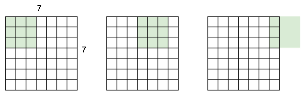
If stride or filter size does not align with the input, parts of the image may not be covered, producing incomplete outputs.
-
The following figure shows how a stride of 3 with a \(7 \times 7\) image and \(3 \times 3\) filter leads to unused edge pixels. In practice, such mismatches are avoided by carefully selecting stride and filter sizes.
Preserving Dimensions with Padding
-
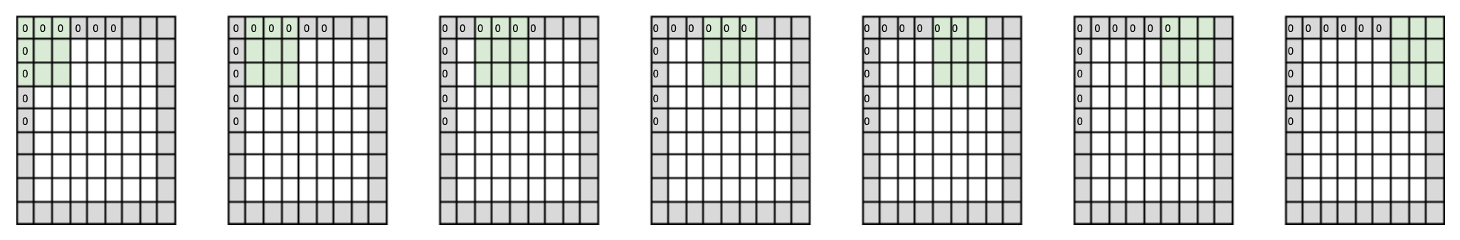
To maintain the same spatial dimensions between input and output, padding is used. Padding adds extra pixels (usually zeros) around the image so that filters can cover the borders fully.
-
For example, adding a 1-pixel border around a \(7 \times 7\) image before applying a \(3 \times 3\) filter at stride 1 yields a \(7 \times 7\) output. This is called a same convolution because the output size equals the input size.
-
The following figure shows how adding padding of 1 before applying a \(3 \times 3\) filter at stride 1 preserves the \(7 \times 7\) dimension. Same convolutions are widely used in architectures like ResNet and U-Net.
Why Controlling Dimensions Matters
-
Managing spatial dimensions is crucial for CNN design:
- If dimensions shrink too quickly, important details may vanish before deep layers extract high-level features.
- If dimensions remain too large, computational and memory costs may explode.
- By adjusting stride and padding, designers balance resolution against efficiency.
-
This careful control of dimensions ensures CNNs remain computationally feasible while still extracting meaningful representations from data.
Padding and Pooling Layers
- While convolutions form the foundation of CNNs, they are almost always combined with padding and pooling to balance spatial resolution, computational cost, and representational power. These layers are critical for making CNNs both efficient and effective.
Padding
-
As discussed earlier, applying convolution without padding reduces the spatial dimensions of the output. If multiple convolutional layers are stacked, this shrinkage compounds, potentially collapsing feature maps too quickly. To address this, CNNs employ padding, which extends the input with additional pixels along the borders.
-
The most common approach is zero-padding, where new pixels are filled with zeros. Zero-padding provides several advantages:
- Preserves spatial dimensions across layers (enabling same convolutions).
- Ensures that edge pixels are treated equally, rather than being underrepresented.
- Allows the construction of deeper networks without rapid shrinking of dimensions.
-
For example, a \(7 \times 7\) input padded with 1 pixel on all sides, followed by a \(3 \times 3\) filter at stride 1, produces a \(7 \times 7\) output. Without padding, the output would shrink to \(5 \times 5\).
Pooling Layers
-
Pooling layers reduce the spatial dimensions of feature maps while retaining the most important information. Unlike convolution, pooling has no trainable parameters—it applies a fixed aggregation operation such as maximum or average.
-
The motivations behind pooling are:
- Dimensionality reduction: reduces memory and computation.
- Translation invariance: small shifts in the input image do not significantly affect outputs.
- Regularization: simplifies intermediate representations and reduces overfitting.
-
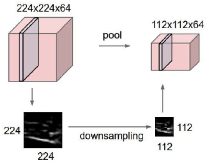
The following figure illustrates how pooling layers shrink and downsample the input. Larger input regions are compressed into smaller outputs, but the dominant features are retained.
Max Pooling
-
The most widely used pooling method is max pooling, which selects the maximum value within each local region. This ensures that the strongest feature is preserved while discarding weaker activations.
-
A common setup uses a \(2 \times 2\) filter with stride 2, which halves both the width and height of the input feature map.
-
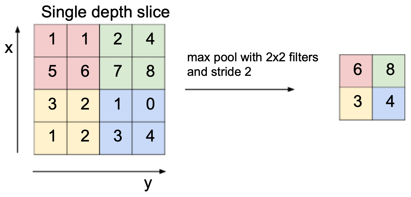
The following figure shows a max pooling operation with a \(2 \times 2\) filter and stride 2 applied to a single depth slice. Each \(2 \times 2\) block reduces to its maximum value, producing a smaller but representative output.
Other Pooling Strategies
-
Although max pooling dominates, other pooling types also play a role in CNN design:
- Average pooling: Computes the mean value within each region. Historically used (e.g., in LeNet), though less effective than max pooling at highlighting salient features.
- Global average pooling: Collapses each entire feature map into a single number by averaging all spatial positions. Frequently used in classification networks (e.g., ResNet) to replace fully connected layers.
- Stochastic pooling: Randomly samples one value from each region, with probability proportional to its magnitude. This introduces beneficial randomness during training.
-
The following figure shows an example of max pooling applied to a \(4 \times 4\) input with a \(2 \times 2\) filter and stride 2, resulting in a reduced \(2 \times 2\) representation. Similar visualizations apply to average or stochastic pooling, where the aggregation differs.
Why Padding and Pooling Work Together
-
Padding and pooling play complementary roles:
- Padding preserves resolution where fine-grained details are important.
- Pooling reduces resolution where abstraction and efficiency are needed.
-
By combining the two, CNNs can carefully manage spatial size across layers—ensuring that networks remain computationally tractable while still retaining rich, hierarchical information.
-
Modern architectures (such as VGGNet, ResNet, and U-Net) systematically apply padding and pooling to balance depth, expressivity, and efficiency.
Advanced CNN Architectures
- As CNNs gained popularity after the success of AlexNet (Krizhevsky et al., 2012), researchers began designing deeper and more efficient architectures. Each new design addressed the challenges of scaling, computation, and representation. These advanced architectures pushed the boundaries of what CNNs could achieve and became the backbone of modern computer vision.
VGGNet: Depth Matters
-
Introduced by Simonyan and Zisserman (2014), VGGNet emphasized the importance of network depth. Instead of using large filters (like 11 × 11 or 7 × 7 in AlexNet), VGG used stacks of small \(3 \times 3\) filters. This choice allowed deeper networks while keeping the number of parameters manageable.
-
Key contributions of VGG:
-
Showed that deeper models significantly improve performance on ImageNet.
-
Standardized the idea of stacking \(3 \times 3\) filters as the core building block.
-
Inspired many later architectures due to its simplicity and uniform design.
-
-
Drawback: Although VGG achieved excellent accuracy, its large number of parameters (over 138 million for VGG-16) made it computationally expensive and memory-intensive.
ResNet: The Shortcut Revolution
-
Deeper networks often suffer from the vanishing gradient problem, where gradients shrink as they propagate backward, making training ineffective. In 2015, ResNet (Residual Networks) by He et al. introduced a breakthrough idea: residual connections (or skip connections).
-
Residual connections allow the network to learn residual functions, enabling effective training of very deep architectures (up to 152 layers in the original paper). This design made it possible to increase depth without degradation in accuracy.
-
Key contributions of ResNet:
-
Introduced the concept of identity mappings via skip connections.
-
Enabled very deep networks that generalize well.
-
Became the foundation for almost all modern CNNs and inspired architectures in other domains (e.g., NLP and speech).
-
Inception Networks: Multi-Scale Feature Extraction
-
Around the same time as ResNet, the Inception architecture (GoogLeNet, Szegedy et al., 2014) explored how to make networks not just deeper, but also wider. Inception modules apply multiple filters of different sizes (\(1 \times 1\), \(3 \times 3\), \(5 \times 5\)) in parallel, then concatenate their outputs. This allows the model to capture features at multiple scales.
-
Key contributions of Inception:
-
Reduced computation using \(1 \times 1\) convolutions as bottleneck layers.
-
Captured multi-scale information effectively.
-
Introduced concepts like auxiliary classifiers for regularization.
-
DenseNet: Feature Reuse
-
Proposed in Huang et al., 2017, DenseNet (Densely Connected Convolutional Networks) extended the idea of ResNet by introducing dense connections. In DenseNet, each layer receives inputs from all previous layers, encouraging feature reuse and alleviating vanishing gradients.
-
Key contributions of DenseNet:
-
Drastically reduced the number of parameters compared to ResNet.
-
Improved gradient flow through dense connections.
-
Encouraged efficient reuse of low-level features in deeper layers.
-
Beyond CNNs: Toward Efficiency and New Paradigms
-
With CNNs becoming larger, researchers also began focusing on efficiency and scalability:
-
MobileNets (Howard et al., 2017): Introduced depthwise separable convolutions, making CNNs efficient for mobile and embedded devices.
-
EfficientNet (Tan & Le, 2019): Used neural architecture search and compound scaling to balance depth, width, and resolution systematically.
-
Vision Transformers (ViTs, Dosovitskiy et al., 2020): Though not CNNs, ViTs represented a paradigm shift by showing that transformer architectures could rival or surpass CNNs in vision tasks when trained on large datasets.
-
CNNs Beyond Classification
-
With these architectures, CNNs rapidly expanded beyond ImageNet classification into diverse tasks:
- Real-time detection: YOLO and SSD for autonomous driving and surveillance.
- Segmentation: Fully Convolutional Networks (FCNs), U-Net, and Mask R-CNN for medical imaging and scene understanding.
- Pose estimation: Detecting human joints and movements for AR/VR and sports analytics.
- Games: Deep CNNs combined with reinforcement learning (e.g., DeepMind’s Atari agents).
- Image captioning: CNNs combined with RNNs or transformers for vision–language tasks.
- Artistic applications: Neural style transfer and generative art.
Legacy of Advanced Architectures
-
The progression from AlexNet to VGG, ResNet, DenseNet, and beyond highlights a common theme: balancing depth, width, efficiency, and generalization. Each innovation—whether deeper stacks of small filters, skip connections, or dense connectivity—has brought us closer to models that are not only accurate but also efficient and scalable.
-
Modern computer vision systems often use these architectures (especially ResNet and EfficientNet) as backbones, fine-tuned for tasks such as detection, segmentation, or generative modeling.
Technical Building Blocks of CNNs
- While convolution and pooling layers form the structural foundation of CNNs, they are not sufficient by themselves to ensure stable and efficient training. Over the years, researchers have developed several critical techniques that make deep CNNs trainable, robust, and generalizable. These include normalization layers, regularization methods like dropout, and advanced optimization strategies.
Normalization Layers
-
As networks become deeper, their internal activations often shift distributions during training, a problem known as internal covariate shift. This makes optimization harder and slows convergence. Normalization layers address this challenge.
-
Batch Normalization (BatchNorm): Introduced by Ioffe & Szegedy, 2015.
- Normalizes layer activations to have zero mean and unit variance across each mini-batch.
- Includes learnable parameters (γ and β) to scale and shift the normalized values.
- Benefits: accelerates convergence, enables higher learning rates, and reduces sensitivity to initialization.
-
Other Variants:
- Layer Normalization (Ba et al., 2016): Normalizes across all features within a single data point; common in NLP.
- Instance Normalization: Often used in style transfer, normalizes per-instance and per-channel.
- Group Normalization (Wu & He, 2018): Divides channels into groups, effective when batch sizes are small.
-
In CNNs, BatchNorm remains the dominant choice, though newer architectures sometimes replace it with alternatives for efficiency.
Dropout
-
Overfitting is a major concern in deep learning, especially when models contain millions of parameters. Dropout, introduced by Srivastava et al., 2014, is a simple yet powerful regularization method.
- During training, dropout randomly “drops” a fraction of neurons (commonly 0.5 in fully connected layers).
- This prevents the network from over-relying on specific neurons, encouraging redundancy and more robust feature learning.
-
At test time, all neurons are active, but their outputs are scaled to account for training-time dropout.
- Dropout is most commonly used in the dense layers of CNNs, though less frequently in convolutional layers, where weight sharing already offers some regularization.
Optimization Strategies
-
CNN training revolves around minimizing a loss function (commonly cross-entropy for classification). The choice of optimization algorithm has a major impact on convergence speed and final accuracy.
-
Stochastic Gradient Descent (SGD):
- The foundational optimizer, updating weights based on gradients from mini-batches.
- Typically paired with momentum (Polyak, 1964), which accumulates a velocity vector to accelerate convergence and smooth updates.
-
Adaptive Methods:
- Adam (Kingma & Ba, 2015): Combines momentum and adaptive learning rates for each parameter. It is widely used because it requires little tuning.
- RMSProp (Tieleman & Hinton, 2012): Adjusts learning rates based on the moving average of squared gradients, stabilizing updates.
-
Learning Rate Schedules:
- Fixed learning rates are rarely optimal.
- Popular schedules include step decay, exponential decay, and cosine annealing (Loshchilov & Hutter, 2016).
- Cyclical learning rates and warm restarts further improve training dynamics by periodically varying learning rates.
Bringing It All Together
-
Modern CNN training pipelines usually combine these elements:
- BatchNorm to stabilize and speed up training.
- Dropout (especially in dense layers) to prevent overfitting.
- Optimizers like SGD with momentum or Adam, often enhanced with dynamic learning rate schedules.
-
Together, these technical building blocks allow CNNs with tens or even hundreds of millions of parameters to train effectively, achieve state-of-the-art accuracy, and generalize well to unseen data.
Applications of CNNs
- The versatility of Convolutional Neural Networks has made them central to modern computer vision. Their ability to automatically learn hierarchical features from raw data allows them to generalize across a wide variety of domains — from everyday tasks like image tagging to life-critical applications in healthcare.
Image Classification
-
The most fundamental application of CNNs is image classification, where the task is to assign a single label to an entire image.
- Datasets and Benchmarks: CNNs rose to prominence through challenges like ImageNet, containing millions of labeled images across 1,000 categories.
-
Practical Uses: Content moderation (e.g., spam or inappropriate image detection), product categorization in retail, and defect detection in manufacturing.
- This success on ImageNet proved that CNNs could generalize beyond curated benchmarks to real-world, noisy image data.
Object Detection
-
Unlike classification, object detection requires both recognizing what objects are present and where they are located.
- Two-Stage Detectors: Models like R-CNN and Faster R-CNN first propose candidate bounding boxes and then classify each. These achieve high accuracy but are computationally expensive.
-
One-Stage Detectors: Models like YOLO (You Only Look Once) and SSD (Single Shot Multibox Detector) perform detection in a single pass, enabling real-time applications.
- Applications: Autonomous driving (detecting cars, pedestrians, and traffic signs), retail analytics (tracking shoppers), and security (surveillance systems).
Semantic and Instance Segmentation
-
For finer-grained understanding, CNNs are used in segmentation, which assigns labels at the pixel level.
- Semantic Segmentation: Every pixel belongs to a category (e.g., sky, road, pedestrian). Architectures include Fully Convolutional Networks (FCNs) and U-Net.
-
Instance Segmentation: Extends semantic segmentation to distinguish between multiple objects of the same category (e.g., two overlapping people). Mask R-CNN is the most widely used model.
- Applications: Self-driving cars (road and lane detection), agriculture (crop monitoring), and medical imaging (tumor segmentation).
Pose Estimation
-
CNNs have also been applied to human pose estimation, where the goal is to detect key points (joints) of the body.
-
Applications: Augmented and virtual reality, sports performance tracking, human–computer interaction, and animation.
Generative Applications
-
CNNs are not limited to recognition—they are also powerful for content generation.
- Neural Style Transfer: Combines the content of one image with the artistic style of another.
-
Generative Adversarial Networks (GANs): Although adversarial training is key, CNN-based generators produce realistic images from random noise.
- The following figure presents a few examples of CNN-driven generative art. These highlight how CNNs can capture texture, structure, and artistic patterns to produce visually striking results.
- Applications: Creative design tools, photorealistic image synthesis, deepfakes, and movie/game asset generation.
Games and Reinforcement Learning
- CNNs have been widely applied in reinforcement learning agents, such as DeepMind’s Atari-playing system (Mnih et al., 2015). By processing raw pixels as input, CNNs allowed agents to learn control policies directly from visual data.
Applications: Robotics, video game AI, and autonomous decision-making systems.
Image Captioning and Vision–Language Tasks
-
CNNs combined with sequence models (RNNs, transformers) enable image captioning: automatically generating textual descriptions of images.
-
Applications: Accessibility tools for the visually impaired, image search engines, and content recommendation.
-
This line of research expanded into vision–language models that combine CNNs or ViTs with large language models, bridging perception and natural language.
Medical Imaging
-
CNNs are among the most impactful tools in healthcare:
- Radiology: Detecting tumors in CT/MRI scans, classifying lung nodules, or identifying fractures.
- Pathology: Distinguishing between cancerous and benign tissue samples.
- Ophthalmology: Screening for diabetic retinopathy using retinal images.
-
While CNNs often achieve human-level accuracy, issues of interpretability, fairness, and regulatory approval remain active areas of research.
Broader Impacts
From self-driving cars to smartphones’ face unlock systems, CNNs now underpin much of modern AI. Their adaptability to both discriminative (classification, detection) and generative (art, synthesis) tasks has made them indispensable across domains like entertainment, security, manufacturing, and healthcare.
Future Directions and Challenges
- Convolutional Neural Networks have reshaped the field of computer vision, but the journey is far from complete. As CNNs continue to evolve, new research themes and practical challenges define the path forward.
Interpretability and Explainability
-
A major criticism of CNNs is their black-box nature. While they achieve remarkable accuracy, understanding why a model makes a particular prediction remains difficult.
- Saliency Maps and Grad-CAM: Visualization methods that highlight which regions of an image most influenced a model’s decision.
-
Explainable AI (XAI): Broader efforts aim to make CNN outputs interpretable to non-experts, which is critical in sensitive domains such as medicine, law, and finance.
- Improving interpretability will increase trust and facilitate safe deployment of CNN-based systems.
Efficiency and Edge Deployment
-
CNNs are computationally intensive, making them challenging to deploy on mobile and embedded devices. Efficiency research has become a key focus:
- Model Compression: Techniques such as pruning, quantization, and knowledge distillation reduce model size without significantly hurting accuracy.
- Lightweight Architectures: Models like MobileNet, ShuffleNet, and EfficientNet are specifically designed for constrained hardware.
- On-Device Inference: Custom accelerators (Google’s TPU, Apple’s Neural Engine) enable CNNs to run on consumer devices in real time.
-
This shift ensures that CNNs can power applications “at the edge,” from AR glasses to autonomous drones.
Fairness, Bias, and Ethics
-
Large-scale datasets used to train CNNs often reflect human and societal biases. These biases can manifest in harmful ways, particularly in high-stakes applications like facial recognition.
- Bias Mitigation: Strategies include dataset balancing, fairness-aware training, and post-processing calibration.
- Ethical Concerns: Applications like surveillance, deepfake generation, and automated decision-making raise critical societal questions.
- Regulation: Policymakers are increasingly scrutinizing AI systems, demanding transparency, accountability, and fairness in CNN deployments.
Hybrid Architectures and the Rise of Transformers
-
The emergence of Vision Transformers (ViTs) has shifted the landscape, showing that self-attention mechanisms can rival or surpass CNNs in vision tasks when trained at scale (Dosovitskiy et al., 2020).
-
Instead of CNNs being replaced, however, a hybrid era is emerging:
- CNN–Transformer Hybrids: Models like DETR (Detection Transformer) combine CNN backbones with transformers to balance local feature extraction and global reasoning.
- Convergence Trend: Future architectures may unify convolution and attention into integrated systems, optimizing both accuracy and efficiency.
Ongoing Research Themes
-
Several promising directions continue to push the boundaries of CNNs:
- Self-Supervised Learning: Reducing reliance on large labeled datasets by using pretext tasks (e.g., predicting missing patches).
- 3D and Video Understanding: Extending CNNs to handle spatiotemporal data for video recognition, action detection, and 3D object modeling.
- Neuromorphic Computing: Exploring biologically inspired CNNs with spiking neurons for ultra-efficient, low-power computation.
- Continual and Few-Shot Learning: Enabling CNNs to adapt to new tasks with minimal labeled data, closer to human learning.
The Road Ahead
-
CNNs ignited the deep learning revolution in vision, and their legacy remains strong. As research advances, CNNs are likely to persist in three complementary roles:
- Standalone architectures in domains where their inductive biases (locality, translation invariance) are advantageous.
- Efficient backbones for downstream tasks in detection, segmentation, and multimodal systems.
- Building blocks in hybrid architectures that merge convolution with attention and beyond.
-
While challenges remain — interpretability, efficiency, fairness, and adaptability — CNNs will continue to shape the future of artificial intelligence, not as isolated tools but as integral components of the broader AI ecosystem.
Citation
If you found our work useful, please cite it as:
@article{Chadha2020ConvolutionalNeuralNetworks,
  title   = {Convolutional Neural Networks},
  author  = {Chadha, Aman},
  journal = {Distilled Notes for Stanford CS231n: Convolutional Neural Networks for Visual Recognition},
  year    = {2020},
  note    = {\url{https://aman.ai}}
}