CS230 • Vulnerabilities of Neural Networks
- Neural networks are vulnerable. Online platforms run powerful neural networks-based classifiers to flag violent or sexual content for removal. A malicious attacker can circumvent these classifiers by introducing imperceptible perturbations on these images, allowing them to live on the platform! This is called an Adversarial Attack.
Attacking Neural Networks with Adversarial Examples
Motivation
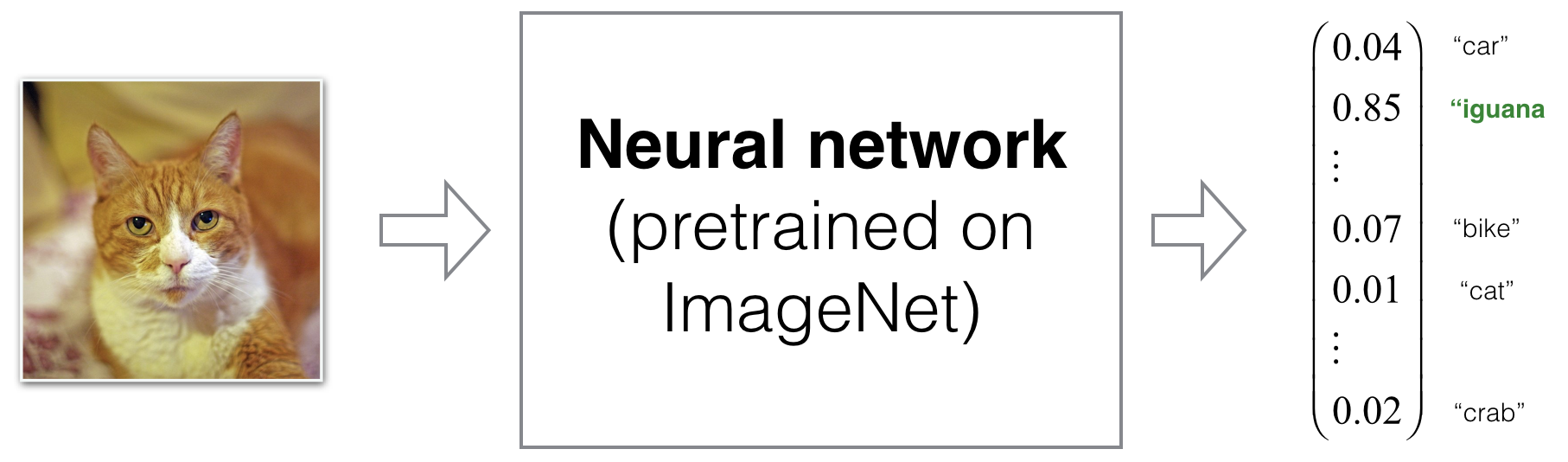
- In 2013, Szegedy et. al identified that it is possible to create a fake datapoint (image 2, text 3 4, speech 5 or even structured data 6) to fool a classifier. In other words, you can generate a fake image that the neural network classifies as a target class you have chosen, for example a cat.
- The generated images might even look real to humans. For instance, an impercetible perturbation on a cat image fools a model to classify it as a cat, while the image still looks like a cat to human.
- These observations have deep consequences on productization neural networks. Here are some examples:
- Autonomous cars use object detectors to localize multiple objects including pedestrians, cars and traffic signs. An imperceptible perturbation of the ‘STOP’ sign image processed by the object detector could a ‘70 miles’ speed limit. This could lead to serious trouble in a real-life setting.
- Face identification systems screen individuals to allow or refuse entrance to a building. A forged image perturbation of an unauthorized person’s face could make this person be authorized.
- Websites run powerful classifiers to detect sexual and violent content online. Imperceptible perturbations of prohibited images could bypass these classifiers and lead to false negative predictions.
- We will first present adversarial attacks, then delve into defenses.
Adversarial Attacks
General procedure
-
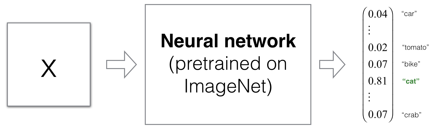
Consider a model pre-trained on ImageNet 7. The following framework is a quick way to forge an example which will be classified as \(i\).
- Pick a sample \(x\) and forward propagate it in the model to get prediction \(\hat{y}\).
- Define a loss function that quantifies the distance between \(\hat{y}\) and the target class prediction \(y_j\). For example: \(\mathcal{L}(\hat{y}, y_j) = \frac{1}{2}||\hat{y} - y_i||^2\).
- While keeping the parameters of the neural network frozen, minimize the defined loss function by updating the pixels of \(x\) iteratively via gradient descent (\(x = x - \alpha \frac{\partial \mathcal{L}}{\partial x}\)). You will find \(x_{adv}\) that is classified as class \(y_i\) with high probability.
-
Because the only constraint in the loss function involved the output prediction, the forged image might be any image from the input space. In fact, the solution of the optimization problem above is much more likely to look random than real. Recall that the size of the space of 32x32 colored images is \(255^{(32 \times 32 \times 3)} \approx 10^{7400}\) which is much larger than the space of 32x32 colored real images.
-
However, you can alleviate that issue by adding a term to the loss that forces the image \(x\) to be close to a chosen image \(x_j\). This is an example of a relevant loss function:
\[\mathcal{L}(\hat{y}, y_j, x) = \frac{1}{2}||\hat{y} - y_i||^2 + \lambda \cdot ||x - x_j||^2\]- where you can tune hyperparameter \(\lambda\) to balance the trade-off between the two terms of the loss expression.
-
After running the optimization process with this procedure, you find an adversarial example that looks like \(x_j\) but is classified as \(y_i\).
In practice
- Using additional tricks such as gradient clipping, you can ensure that the difference between the generated image and the target image (\(x_j\)) are imperceptible.
Defenses to adversarial attacks
Types of attacks
- There are two types of attacks:
- white-box: The attacker has access to information about the network.
- black-box: The attacker does not have access to the network, but can query it (i.e. send inputs and observe predictions.)
- In the optimization above, computing \(\frac{\partial \mathcal{L}}{\partial x}\) using backpropagation requires access to the network weights. However, in a black-box setting, you could approximate the gradient by making tiny changes to the input and observing the output (\(\frac{\partial \mathcal{L}}{\partial x} ≈ \frac{f(x+\varepsilon) - f(x)}{(x + \varepsilon) - x}\)).
Defense methods
- Defenses against adversarial attacks is an important research topic. Although no method have been proven to counter all attacks yet, the following directions have been proposed:
- Create a SafetyNet acting as a FireWall to stop adversarial examples from fooling your model. SafetyNet should be hard to optimized such that it is difficult to produce examples that are both misclassified and slip past SafetyNet’s detector.
- Add correctly labelled adversarial examples to the training set. This consists of simply training the initial network with additional examples to force the representation of each class to take into account small perturbations.
- Use Adversarial training. For each example fed to your network, the loss also takes into account the prediction of a perturbation \(x_{adv}\) of the input \(x\) of label \(y\). In other words, by calling \(\mathcal{L}\) the ‘normal’ loss of the network, \(W\) its parameters, a possible candidate for the new loss can be given by \(L(W,x,y) + \lambda L(W,x_{adv}, y)\). Here, \(\lambda\) is a hyperparameter that balances model robustness versus performance towards real data.
- Note that (2) and (3) are computationally expensive using the iterative method of generating adversarial example. In the next part, you will learn a method called Fast Gradient Sign Method (FGSM) which generates adversarial examples in one pass.
Why are neural networks vulnerable to adversarial examples?
Example: Adversarial attack on logistic regression
-
Consider a logistic regression defined by: \(\hat{y} = \sigma{Wx + b}\)$, where \(x \mapsto \sigma(x)\) indicates the sigmoid function. The shapes are: \(x \in \mathbb{R}^{n \times 1}\)$, \(W \in \mathbb{R}^{1 \times n}\) and \(\hat{y} \in \mathbb{R}^{1 \times 1}\). For simplicity, assume \(b = 0\) and \(n = 6\).
-
Let \(W = (1, 3, -1, 2, 2, 3)\) and \(x = (1, -1, 2, 0, 3, -2)^T\). In this setting, \(\hat{y} = 0.27\). This means that with \(73\%\) probability, the predicted class is \(y = 0\).
-
Now, how can you change \(x\) slightly and convert the model’s prediction to \(y = 1\)? One way is to move components of \(x\) in the same direction as \(sign(W)\). By doing this, you ensure that the perturbations will lead to a positive addition to \(\hat{y}\).
-
\(x_{adv} = x + \varepsilon sign(W) = (1, -1, 2, 0, 3, -2)^T + (0.4, 0.4, -0.4, 0.4, 0.4, 0.4) = (1.4, -0.6, 1.6, 0.4, 3.4, -1.6)\) for \(\epsilon = 0.4\) leads to \(\hat{y} = \sigma{Wx_{adv} + b} = \sigma (1, 3, -1, 2, 2, 3) \cdot (1.4, -0.6, 1.6, 0.4, 3.4, -1.6) = \sigma(1.4 - 1.8 - 1.6 + 0.8 + 6.8 - 4.8) = \sigma(0.8) = 0.69\). The prediction is now \(y = 1\) with 69% confidence.
-
This small example illustrates that a rightly chosen \(\epsilon\)-perturbation can have a considerable impact on the output of a neural network.
Comments
- Despite being less powerful, using \(\varepsilon sign(W)\) instead of \(\varepsilon W\) ensures that \(x_{adv}\) stays close to \(x\). The perturbation is indeed capped by \(\varepsilon\).
- The larger \(n\)$, the more powerful the attack. Indeed, perturbating each feature of \(x\) additively impacts \(\hat{y}\).
- For neural networks, \(x_{adv} = x + \varepsilon sign(W)\) can be generalized to \(x_{adv} = x + \varepsilon sign(\nabla_x \mathcal{L}(W,x,y))\). The intuition is that you want to push \(x\) with limited amplitude in the direction of positive changes of the loss function. This method is called the Fast Gradient Sign Method (FGSM). It generates adversarial examples much faster than the iterative method described earlier.
Conclusion
- Although early attempts at explaining the existence of adversarial examples focused on overfitting and network non-linearity, Goodfellow et al. (in Explaining and Harnessing Adversarial Examples [cite]) found that it is due to the linearity of the network. Indeed, neural networks have been designed to behave linearly (think about the introduction of ReLU, LSTMs, etc.) in order to ease to optimization process. Even activation functions such as \(\sigma\) and \(tanh\) have been designed to function in their linear regime with methods such as Xavier Initialization and BatchNorm. However, the FGSM illustrates that easy-to-train models are easy-to-attack because the gradients can backpropagate.
Further readings
- If you’re looking for a survey of adversarial examples, Yuan et al. offer a review of recent findings on adversarial examples for deep neural networks.
- If you are more interested in adversarial attack and defense scenarios, Kurakin et al. is a great supplement.