CS230 • Sequence Models
- Sequence models: motivation, notation, and problem formulations
- Why sequences matter
- A running example: named entity recognition (NER)
- Representing tokens: vocabulary and one-hot encoding
- The recurrent modeling idea
- Loss functions and sequence-level objectives
- Many-to-one, one-to-many, and many-to-many patterns
- Practicalities of tokenization and unknowns
- Reading guide and context within the literature
- Recurrent neural networks: fundamentals and training
- Variations of recurrent neural networks and their applications
- Many-to-one: sequence classification
- One-to-many: conditional generation
- Many-to-many (aligned): per-step labeling
- Many-to-many (unaligned): sequence-to-sequence
- Language modeling
- Sampling novel sequences
- Ambiguity resolution via context: language modeling example
- Character-level vs. word-level modeling
- Limitations of vanilla RNNs
- Vanishing and exploding gradients in RNNs
- Gated recurrent units (GRUs)
- Long short-term memory (LSTM) networks
- Bidirectional recurrent neural networks (BRNNs)
- Deep recurrent neural networks (Deep RNNs)
- Word embeddings and word representations
- Learning word embeddings
- From static to contextual embeddings
- Citation
Sequence models: motivation, notation, and problem formulations
- Sequence models are the family of statistical and neural architectures designed to map between sequences whose lengths may vary across examples. This flexibility underpins a remarkably broad range of tasks where either the inputs, the outputs, or both, are ordered collections with variable cardinality. In contrast to fixed-size feed-forward architectures, sequence models explicitly encode temporal or structural dependencies via recurrent computation, attention, or convolution over sequence positions.
Why sequences matter
-
In many real-world problems, the object of interest is not a single vector but an ordered list \(x^{\langle 1\rangle}, x^{\langle 2\rangle}, \dots, x^{\langle T_x\rangle}\). The ordering carries meaning: phonemes form words, nucleotides form genes, frames form actions. Sequence models aim to learn a conditional distribution over outputs that respects this order:
\[p\!\left(y^{\langle 1:T_y\rangle}\mid x^{\langle 1:T_x\rangle}\right)\]- where \(T_x\) and \(T_y\) may differ and vary across training examples.
-
Below are representative application modalities that benefit from this formulation.
- Speech recognition maps an acoustic sequence to a token sequence; \((T_x \neq T_y)\) and both vary.
- Music generation conditions on metadata or a seed motif and emits a note sequence; typically one-to-many.
- Sentiment classification ingests a sentence and produces a single label; many-to-one.
- DNA sequence analysis takes a nucleotide string and produces per-position annotations (e.g., protein-coding regions); many-to-many with aligned lengths.
- Machine translation transforms a source sentence into a target sentence; many-to-many with different lengths.
- Video activity recognition consumes a sequence of frames and outputs an action label; many-to-one or many-to-many depending on granularity.
- Named entity recognition (NER) labels each token as being part of an entity or not; many-to-many with equal lengths.
A running example: named entity recognition (NER)
- Consider the input sentence:
-
Let \(x^{\langle t\rangle}\) denote the \(t^{th}\) token (1-indexed). For NER, a convenient target is a per-token binary (or multi-hot) label \(y^{\langle t\rangle}\in\{0,1\}^K\). In the simplest binary case \(K=1\) indicating whether a token is part of a named entity. For the sentence above, one possible target is:
\[y = [1,\ 1,\ 0,\ 1,\ 1,\ 0,\ 0,\ 0,\ 0]\]- where positions corresponding to Harry, Potter, Hermione, and Granger are marked positive. We denote input length by \(T_x\) and output length by \(T_y\). In aligned labeling tasks like this, \(T_x=T_y=9\), but in general \(T_x\) and \(T_y\) can differ.
-
For a dataset of examples indexed by \(i\), we allow per-example lengths \(T_x^{(i)}\) and \(T_y^{(i)}\).
Representing tokens: vocabulary and one-hot encoding
-
To operate on words, we compile a vocabulary \(V\) of size \(\|V\|\) (often \(10^4\)–\(10^5\) in modern applications). Each token \(x^{\langle t\rangle}\) is represented as a one-hot vector \(e(x^{\langle t\rangle})\in\{0,1\}^{\|V\|}\) with a single 1 at the index of the token in the sorted vocabulary and 0 elsewhere. Tokens not present in \(V\) map to a special unknown token \(\langle \text{UNK}\rangle\). End-of-sentence \(\langle \text{EOS}\rangle\) and other control tokens are commonly included.
-
One-hot encodings are simple and lossless with respect to vocabulary identity, but they do not express semantic similarity: vectors for “apple” and “orange” are orthogonal despite their obvious relationship. Later, we will introduce distributed word representations (embeddings) that remedy this limitation.
The recurrent modeling idea
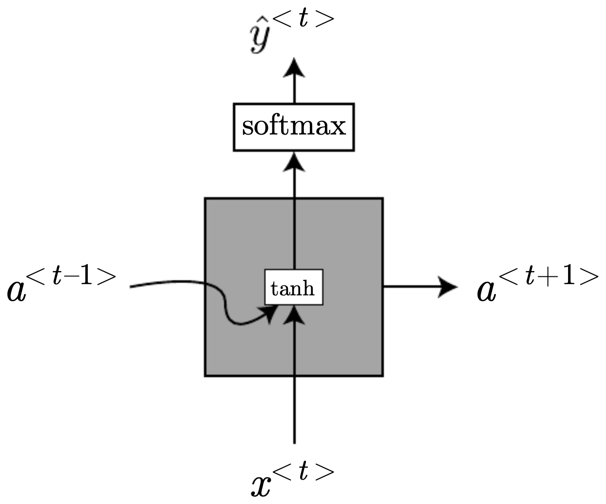
- A basic recurrent neural network (RNN) defines a latent state \(a^{\langle t\rangle}\in\mathbb{R}^H\) that summarizes the past, updating it with the current input:
-
with \(a^{\langle 0\rangle}=\mathbf{0}\) by convention, \(g(\cdot)\) typically \(\tanh\) or \(\text{ReLU}\), and \(\phi(\cdot)\) chosen to match the prediction head (sigmoid for binary labels, softmax for multi-class). It is convenient to write the input-augmented linear map as
\[a^{\langle t\rangle} = g\!\left(W_a\,[\,a^{\langle t-1\rangle};\,x^{\langle t\rangle}\,] + b_a\right), \qquad \hat{y}^{\langle t\rangle} = \phi\!\left(W_{y}\,a^{\langle t\rangle} + b_y\right)\]- where \([\,\cdot;\cdot\,]\) denotes concatenation.
-
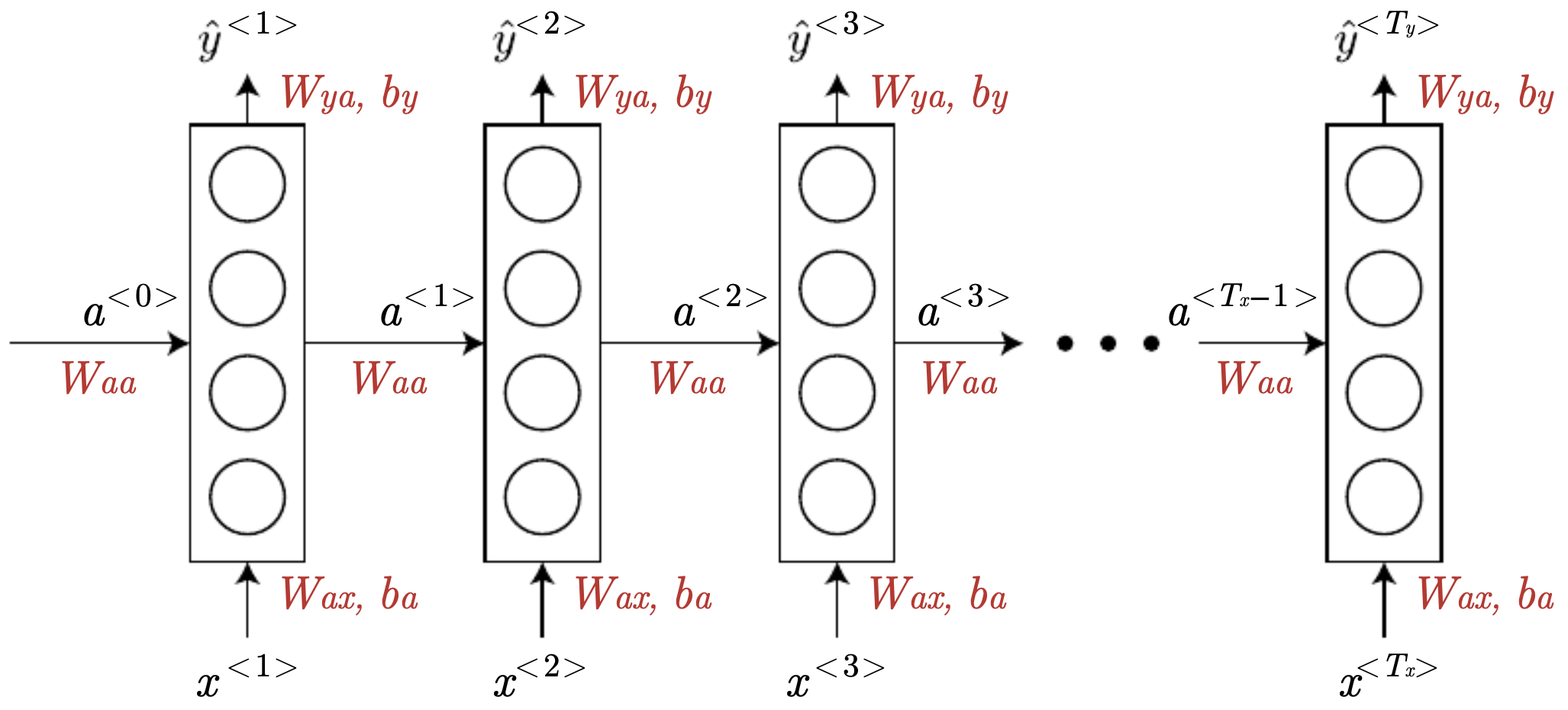
The central inductive bias is parameter sharing across time: the same \(W_a\) and \(W_y\) are reused at every step, allowing the model to generalize across sequence positions and lengths.
-
The following figure depicts a basic RNN unrolled across time: each cell consumes \(x^{\langle t\rangle}\), updates the hidden state \(a^{\langle t\rangle}\), and predicts \(\hat{y}^{\langle t\rangle}\). Red-highlighted matrices indicate parameters shared at all time steps. The figure emphasizes the repeated application of the same parameters over time and the dependence of \(\hat{y}^{\langle t\rangle}\) on both current input and the aggregated past.
Loss functions and sequence-level objectives
- For many-to-many labeling (e.g., NER), a natural objective is the sum of per-time-step cross-entropies:
- For language modeling, where the task is to assign probability to a sequence \(y^{\langle 1:T\rangle}\), the chain rule factorization is
- … and the training objective is the negative log-likelihood (sum of token-level cross-entropies with teacher forcing).
Many-to-one, one-to-many, and many-to-many patterns
-
Different supervision patterns arise depending on the mapping between input and output sequences:
- Many-to-one: Aggregate an entire input sequence to a single prediction \(y\) (e.g., sentiment analysis). One uses the final state \(a^{\langle T_x\rangle}\) or a pooled summary to predict \(y\).
- One-to-many: Condition on a fixed context vector \(x\) and generate a sequence (e.g., music generation); the context seeds the initial state, and the model rolls out predictions autoregressively.
- Many-to-many (aligned): Emit a label per input position with the same length (e.g., NER, CTC-free phone labeling).
- Many-to-many (unaligned): Map between sequences of different lengths (e.g., machine translation), typically with encoder–decoder architectures.
-
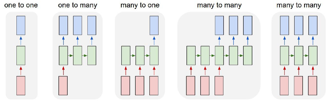
The following figure contrasts one-to-one, one-to-many, many-to-one, and many-to-many sequence mappings, emphasizing when input and output lengths match or differ and where recurrence appears. The idea behind sketching these canonical patterns is to help readers map a problem to an appropriate recurrent topology before diving into model variants.

Practicalities of tokenization and unknowns
-
In textual tasks, tokenization choices (word-level vs. character-level vs. subword/BPE) affect \(T_x\), vocabulary size, and the unknown-token rate. Word-level models require an \(\langle \text{UNK}\rangle\) token but can struggle with rare words and morphology. Character-level models eliminate \(\langle \text{UNK}\rangle\) at the cost of longer sequences and weaker long-range modeling with simple RNNs. Subword schemes (e.g., BPE, unigram LM) offer a compromise by composing words from a learned set of frequent chunks.
-
For our running examples in this primer, we will initially assume word-level inputs with one-hot vectors and later transition to dense embeddings learned from large corpora, which transfer effectively to downstream tasks.
Reading guide and context within the literature
-
Classic recurrent modeling dates back to early work on simple recurrent networks Elman (1990). Long short-term memory (LSTM) introduced gating to mitigate vanishing gradients Hochreiter & Schmidhuber (1997), while gated recurrent units (GRUs) proposed a streamlined alternative Cho et al. (2014). Bidirectional RNNs incorporate both past and future context for per-position predictions Schuster & Paliwal (1997). We will build up to these variants from the basic RNN formulation above.
-
The next section will dive into forward computation, the training objective in detail, and backpropagation through time (BPTT), including computational graphs and common pitfalls such as exploding/vanishing gradients.
Recurrent neural networks: fundamentals and training
- Having established the motivation and notation for sequence models, we now turn to the simplest recurrent formulation: the vanilla RNN. We will examine its forward dynamics, its objective, and the mechanics of backpropagation through time (BPTT). Along the way, we will see both the power and the limitations of this basic architecture.
Forward dynamics of a simple RNN
- At each time step \(t\), the network maintains a hidden state vector \(a^{\langle t\rangle}\) that aggregates past information. It evolves recursively:
-
with \(a^{\langle 0\rangle}=\mathbf{0}\). The predicted output at the same step is
\[\hat{y}^{\langle t\rangle} = \phi\!\left(W_{ya}a^{\langle t\rangle} + b_y\right)\]-
where:
- \(W_{aa}\in \mathbb{R}^{H\times H}\) governs recurrence,
- \(W_{ax}\in \mathbb{R}^{H\times \|V\|}\) projects the input,
- \(W_{ya}\in \mathbb{R}^{\|O\|\times H}\) maps hidden states to outputs,
- \(g\) is typically \(\tanh\) or ReLU,
- \(\phi\) is task-dependent (sigmoid, softmax).
-
-
The compact notation
-
with concatenation \([\,;\,]\), emphasizes parameter sharing across all time steps.
-
The following figure illustrates this unrolling, highlighting the shared parameters/matrices in red (\(W_{aa}, W_{ax}, W_{ya}\)) are reused identically at every step. Put simply, each block consumes the current input and previous hidden state to produce an output.
Sequence-level loss
- At each step \(t\), the local loss is
- Aggregating over a sequence of length \(T_y\):
- For categorical outputs with vocabulary size \(\|V\|\), \(\hat{y}^{\langle t\rangle}\) is a softmax distribution and \(\mathcal{L}^{\langle t\rangle}\) is cross-entropy.
Backpropagation through time (BPTT)
-
Training requires gradients with respect to recurrent weights. Unlike feed-forward nets, RNNs reuse parameters at each time step. To compute gradients, we unroll the recurrence over \(T_x\) steps, yielding a deep computational graph of depth proportional to sequence length.
-
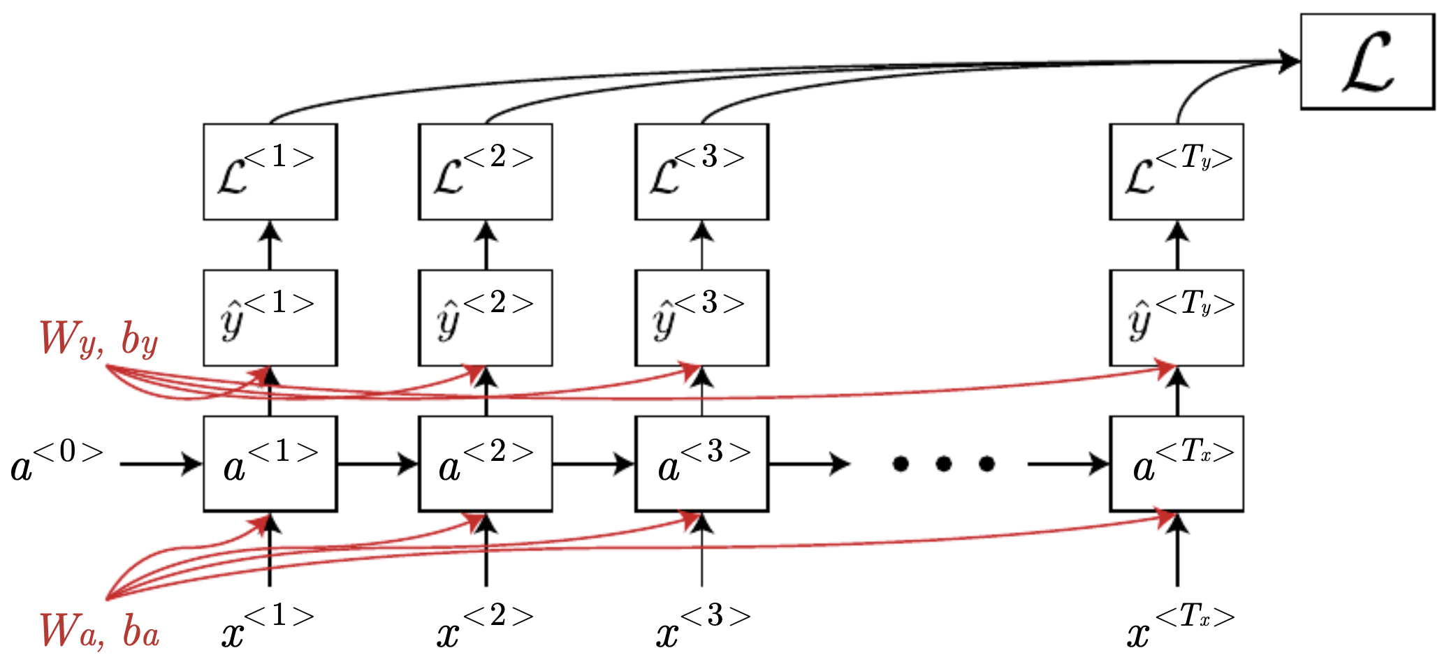
The loss gradient backpropagates through this unrolled graph, step by step, in reverse order. This is termed backpropagation through time (BPTT). Crucially, the same weight matrices accumulate gradient contributions from all time steps:
- The following figure depicts the computational graph for an RNN unrolled across time. Gradients, represented by the backward arrows, flow backwards step-by-step during backpropagation through time, with recurrent parameters accumulating contributions across all steps.
Challenges with simple RNNs
-
While conceptually elegant, vanilla RNNs face serious optimization obstacles:
- Exploding gradients: products of Jacobians can blow up exponentially, causing unstable updates.
- Vanishing gradients: conversely, repeated multiplication by small derivatives shrinks gradients, impairing learning of long-term dependencies.
-
Limited memory: because information must persist via repeated transformations of \(a^{\langle t\rangle}\), signals about distant inputs often dissipate.
- These challenges motivate architectural innovations—most famously gated mechanisms like GRUs and LSTMs—that we will cover in subsequent sections.
Variations of recurrent neural networks and their applications
- The vanilla RNN provides a general template for processing sequences, but different tasks require different input–output alignments. Here, we explore the main variants: many-to-one, one-to-many, many-to-many, and language modeling. We will also discuss sequence sampling and the limits of vanilla RNNs in practice.
- The following figure depicts different types of RNNs based on the combinations of fixed or variable length input and output.
Many-to-one: sequence classification
- In many tasks, the goal is to map an entire input sequence to a single output. Examples include sentiment classification, activity recognition, or spam detection. Here, the model consumes the sequence and aggregates information in the hidden state:
- Only the final hidden state is used for prediction. While simple, this approach risks losing information about earlier inputs if the hidden state cannot retain long-range dependencies.
One-to-many: conditional generation
- Conversely, in tasks such as music generation or image captioning, a fixed input (e.g., a genre label or an image embedding) conditions the generation of a sequence. The input initializes the hidden state \(a^{\langle 0\rangle}\), and the network autoregressively emits outputs:
- This setup is one-to-many because a single context vector seeds multiple outputs.
Many-to-many (aligned): per-step labeling
-
When input and output lengths match, we predict a label for each time step. Examples include:
- Part-of-speech tagging
- Named entity recognition
- Frame-level activity detection in video
-
The RNN outputs \(\hat{y}^{\langle t\rangle}\) at each time step, with losses summed over all steps.
Many-to-many (unaligned): sequence-to-sequence
-
In machine translation, speech-to-text, or summarization, input and output sequences differ in length. Encoder–decoder architectures address this: an encoder RNN compresses the input sequence into a latent vector, which initializes a decoder RNN that generates the output sequence.
-
This paradigm underlies modern sequence-to-sequence learning, later enhanced by attention and transformers.
Language modeling
- Language models estimate the probability of a sequence of words. Given a sentence \(y^{\langle 1:T\rangle}\), an RNN language model factorizes its likelihood as
-
At training time, the input at step \(t\) is the true token \(y^{\langle t-1\rangle}\) (teacher forcing). At inference, the model uses its own predictions autoregressively.
-
Example:
- Input: “Well, hello …”
- At \(t=1\): \(\hat{y}^{\langle 1\rangle}\) is a distribution over 10k words; the true token is “Well”.
- At \(t=2\): conditioned on “Well”, the model predicts the next word, ideally “hello”.
- At \(t=3\): conditioned on “Well, hello”, it predicts “there”.
-
The training objective maximizes the log-likelihood of the observed sequence:
Sampling novel sequences
-
To generate text, we start with a special
token, then repeatedly: - Feed the previous prediction into the RNN.
- Sample from the output distribution (using multinomial sampling to avoid deterministic loops).
- Stop when an
token is produced or after a maximum length.
-
This procedure allows creative sequence generation in text, music, or DNA motifs.
-
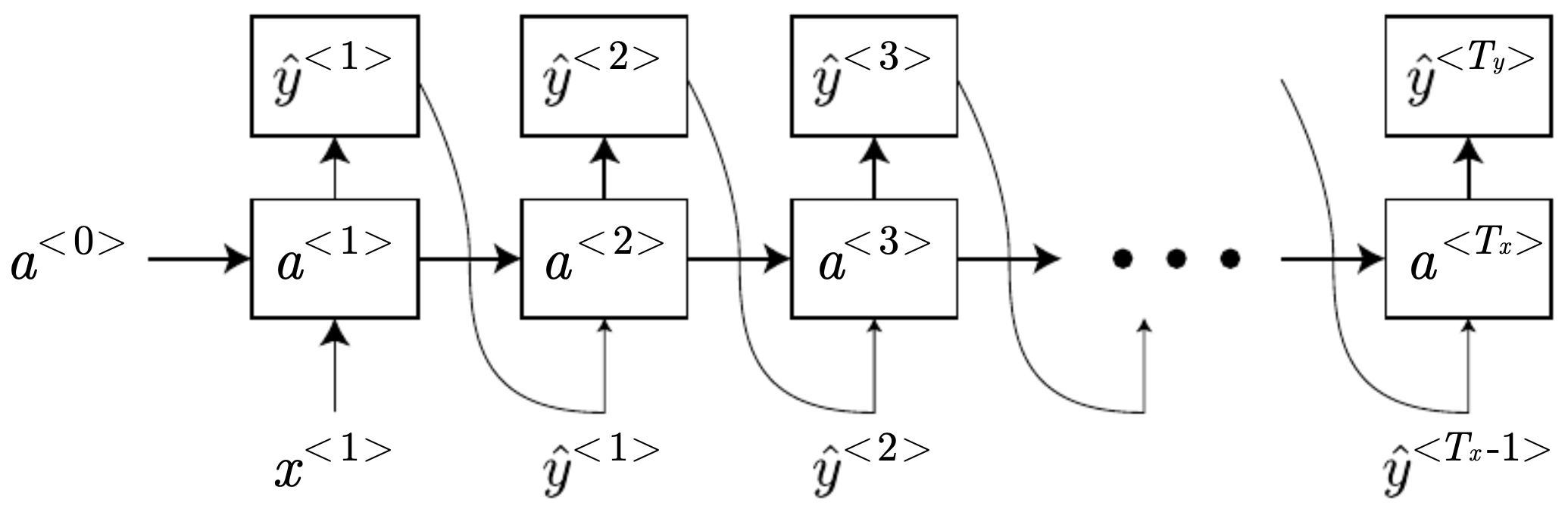
The following figure illustrates sequence generation with an RNN, where each predicted token is fed back as the input to the next time step until an end-of-sequence token is produced.
Ambiguity resolution via context: language modeling example
-
Pronunciation alone cannot distinguish homophones (e.g., “pear” vs. “pair”). A language model uses context to select the more plausible option:
- “The apple and pear salad” vs. “The apple and pair salad”.
-
Though acoustically identical, the second is less probable given training statistics. Formally:
- Thus, sequence models enable disambiguation by leveraging contextual dependencies across time.
Character-level vs. word-level modeling
- Word-level models: efficient, better at capturing long-range semantics, but require an
token for out-of-vocabulary words. - Character-level models: no
, capture morphology naturally, but struggle with long dependencies and are computationally heavier.
Limitations of vanilla RNNs
-
As sequence length grows, vanilla RNNs fail to preserve information across long spans. This is due to:
- Vanishing gradients (exponential decay of signal).
- Exploding gradients (exponential growth of signal).
- Difficulty modeling hierarchical dependencies.
-
These issues necessitate gated mechanisms (GRUs, LSTMs) and bidirectional extensions, which we will explore next.
Vanishing and exploding gradients in RNNs
- While recurrent neural networks elegantly handle variable-length inputs, their training is notoriously difficult for long sequences. The root cause is the behavior of gradients as they are propagated backward through time. Here, we analyze the mathematics behind vanishing and exploding gradients, their consequences, and mitigation strategies.
Gradient propagation in RNNs
- Consider the recurrence:
- … with hidden state dimension \(H\). For simplicity, assume a linear activation \(g(z)=z\). Then:
- Unrolling over \(t\) steps:
- Thus, the state depends on powers of \(W_{aa}\). During backpropagation, gradients also accumulate factors of \(W_{aa}^T\).
The vanishing/exploding effect
-
The gradient of the loss with respect to an earlier hidden state has the form:
\[\frac{\partial \mathcal{L}}{\partial a^{\langle t\rangle}} = \left(\prod_{k=t+1}^{T} W_{aa}^\top D^{\langle k\rangle}\right)\frac{\partial \mathcal{L}}{\partial a^{\langle T\rangle}}\]- where \(D^{\langle k\rangle}\) is the diagonal Jacobian of the activation \(g\).
-
Key insight: the product of many matrices tends either to shrink to zero (vanishing gradient) or to blow up (exploding gradient), depending on the spectral radius \(\rho(W_{aa})\).
- If \(\rho(W_{aa}) < 1\), gradients decay exponentially with time steps.
- If \(\rho(W_{aa}) > 1\), gradients grow exponentially.
- If \(\rho(W_{aa}) \approx 1\), training remains unstable but somewhat more balanced.
Consequences for learning
-
Vanishing gradients: The network struggles to assign credit to inputs that occurred many steps earlier. This impairs learning of long-term dependencies such as subject–verb agreement or open–close bracket matching.
-
Exploding gradients: Training becomes numerically unstable, with weight updates overshooting. Loss may oscillate or diverge.
Practical manifestations
-
Imagine training an RNN to predict the correct verb form in the sentence:
- “The cat, which already ate, was full.”
- vs. “The cats, which already ate, were full.”
-
To get the verb right, the model must carry information about the subject across many words. A vanilla RNN with vanishing gradients cannot propagate this signal reliably.
Mitigation strategies
- Several practical methods exist to combat gradient instability:
- Gradient clipping:
- Before parameter updates, rescale gradients if their norm exceeds a threshold:
- This prevents exploding updates.
- Careful initialization:
- Orthogonal or identity initialization of \(W_{aa}\) can help keep \(\rho(W_{aa})\) close to 1.
- Activation functions:
- Saturating activations (sigmoid, tanh) exacerbate vanishing. ReLU partially alleviates this, though it introduces other issues (dying ReLUs).
- Architectural innovations:
- Gated architectures (GRUs, LSTMs) introduce explicit memory mechanisms that enable better gradient flow.
- The following figure shows an RNN hidden state represented as a black box at each time step. The figure specifically illustrates the failure of vanilla RNNs to capture long-term dependencies. The hidden state must preserve information across many time steps, but the gradients either shrink or explode, preventing stable training. As the sequence grows, the network struggles to preserve information about early tokens, illustrating the vanishing gradient problem.
From limitations to solutions
- While gradient clipping and careful initialization help, they do not solve the fundamental problem: vanilla RNNs cannot maintain stable memory across long sequences. This motivates gated recurrent architectures, most notably the GRU and LSTM, which introduce explicit mechanisms for memory retention and controlled information flow.
Gated recurrent units (GRUs)
- Gated recurrent units (GRUs), introduced by Cho et al. (2014), were designed to address the vanishing gradient problem in vanilla RNNs. They introduce gating mechanisms that control how much information flows through the hidden state, allowing the network to preserve relevant long-term dependencies while efficiently discarding irrelevant information.
Intuition behind GRUs
-
A vanilla RNN compresses all past information into a single vector \(a^{\langle t\rangle}\). This single update rule makes it difficult to remember information over long spans: gradients vanish, and the network forgets too quickly.
-
GRUs augment this with two gates:
- Update gate \(u^{\langle t\rangle}\): decides how much of the past hidden state to keep vs. how much to replace with new candidate information.
- Reset gate \(r^{\langle t\rangle}\): decides how much of the past hidden state is relevant for computing the new candidate.
-
These gates are differentiable functions of the input and previous hidden state, trained jointly with the model.
GRU equations
-
For input \(x^{\langle t\rangle}\) and previous hidden state \(a^{\langle t-1\rangle}\):
-
Update gate:
\[u^{\langle t\rangle} = \sigma\!\left(W_u \,[a^{\langle t-1\rangle}, x^{\langle t\rangle}] + b_u\right)\] -
Reset gate:
\[r^{\langle t\rangle} = \sigma\!\left(W_r \,[a^{\langle t-1\rangle}, x^{\langle t\rangle}] + b_r\right)\] -
Candidate hidden state:
\[\tilde{a}^{\langle t\rangle} = \tanh\!\left(W_a \,[r^{\langle t\rangle} \odot a^{\langle t-1\rangle}, x^{\langle t\rangle}] + b_a\right)\] -
Final hidden state update:
\[a^{\langle t\rangle} = u^{\langle t\rangle} \odot \tilde{a}^{\langle t\rangle} + \left(1 - u^{\langle t\rangle}\right) \odot a^{\langle t-1\rangle}\]
- where \(\odot\) denotes elementwise multiplication.
-
Intuitive behavior of the gates
- If \(u^{\langle t\rangle} \approx 1\): the model replaces the hidden state with the new candidate, forgetting old information.
- If \(u^{\langle t\rangle} \approx 0\): the hidden state is preserved, carrying past information forward.
-
If \(r^{\langle t\rangle} \approx 0\): the reset gate blocks past information, allowing the candidate to depend only on the new input.
- This flexibility enables GRUs to retain information over long sequences while remaining computationally efficient.
Example: singular vs. plural consistency
-
Consider the sentence:
- “The cat, which already ate, was full.”
- “The cats, which already ate, were full.”
-
For correct verb agreement, the model must remember whether the subject was singular or plural. A GRU can maintain this information by setting the update gate low (\(u^{\langle t\rangle} \approx 0\)) across many time steps, ensuring that the subject information persists until the verb.
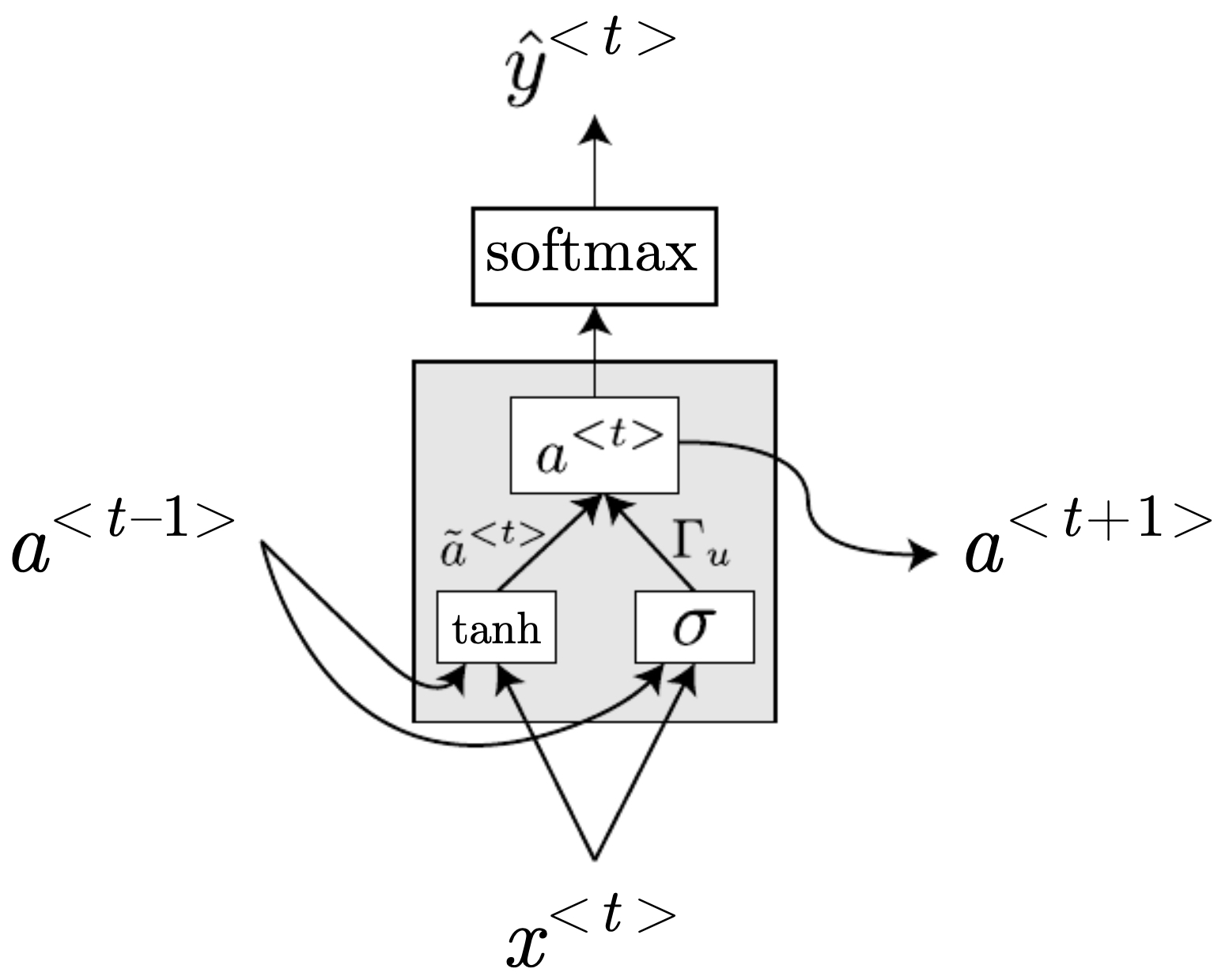
GRU computational graph
- The following figure illustrates a GRU cell at a single time step, highlighting the gating structure: inputs flow through reset and update gates, controlling how the hidden state is updated and carried forward.
Advantages of GRUs
- Fewer parameters than LSTMs (no separate memory cell).
- Efficient to train, often faster convergence.
- Effective at capturing dependencies spanning dozens of time steps.
- Widely used in speech recognition, machine translation (pre-attention era), and time-series modeling.
Limitations of GRUs
- May struggle with very long-term dependencies compared to LSTMs.
- Lacks explicit memory cell, which limits interpretability.
- In some tasks, performance lags behind LSTMs, especially when extremely long contexts are needed.
Long short-term memory (LSTM) networks
- Long short-term memory (LSTM) networks, introduced by Hochreiter & Schmidhuber (1997), extend the idea of gated recurrence by introducing a separate memory cell that can carry information across very long time spans. This makes them one of the most powerful architectures for sequence modeling, widely used before the advent of attention-based transformers.
Motivation
-
While GRUs improve gradient flow by controlling when to update or reset hidden states, they still merge memory and hidden state into a single vector. LSTMs separate these roles:
- Cell state (\(c^{\langle t\rangle}\)): a dedicated memory vector designed to preserve information over long time spans.
- Hidden state (\(h^{\langle t\rangle}\)): the exposed representation used for predictions.
-
This separation allows gradients to flow more smoothly across time, mitigating vanishing gradients.
Core components of an LSTM cell
-
At each time step \(t\), the LSTM maintains two vectors: the cell state \(c^{\langle t\rangle}\) and the hidden state \(h^{\langle t\rangle}\). Updates are governed by three gates:
- Forget gate: decides what to discard from the cell state.
- Update (input) gate: decides what new information to add.
- Output gate: decides what part of the cell state to reveal as hidden state.
LSTM equations
-
For input \(x^{\langle t\rangle}\), previous hidden state \(h^{\langle t-1\rangle}\), and previous cell state \(c^{\langle t-1\rangle}\):
-
Forget gate:
\[f^{\langle t\rangle} = \sigma\!\left(W_f \,[h^{\langle t-1\rangle}, x^{\langle t\rangle}] + b_f\right)\] -
Update gate:
\[u^{\langle t\rangle} = \sigma\!\left(W_u \,[h^{\langle t-1\rangle}, x^{\langle t\rangle}] + b_u\right)\] -
Candidate cell state:
\[\tilde{c}^{\langle t\rangle} = \tanh\!\left(W_c \,[h^{\langle t-1\rangle}, x^{\langle t\rangle}] + b_c\right)\] -
Cell state update:
\[c^{\langle t\rangle} = f^{\langle t\rangle} \odot c^{\langle t-1\rangle} + u^{\langle t\rangle} \odot \tilde{c}^{\langle t\rangle}\] -
Output gate:
\[o^{\langle t\rangle} = \sigma\!\left(W_o \,[h^{\langle t-1\rangle}, x^{\langle t\rangle}] + b_o\right)\] -
Hidden state update:
\[h^{\langle t\rangle} = o^{\langle t\rangle} \odot \tanh\!\left(c^{\langle t\rangle}\right)\]
-
Intuitive role of the gates
- Forget gate (\(f^{\langle t\rangle}\)): If \(f^{\langle t\rangle} \approx 1\), old information in \(c^{\langle t-1\rangle}\) is preserved; if close to 0, it is erased.
- Update gate (\(u^{\langle t\rangle}\)): Controls how much new candidate information enters the cell state.
-
Output gate (\(o^{\langle t\rangle}\)): Decides which parts of the memory should affect the hidden state (and thus the prediction).
- Together, these gates allow selective remembering, forgetting, and revealing of information.
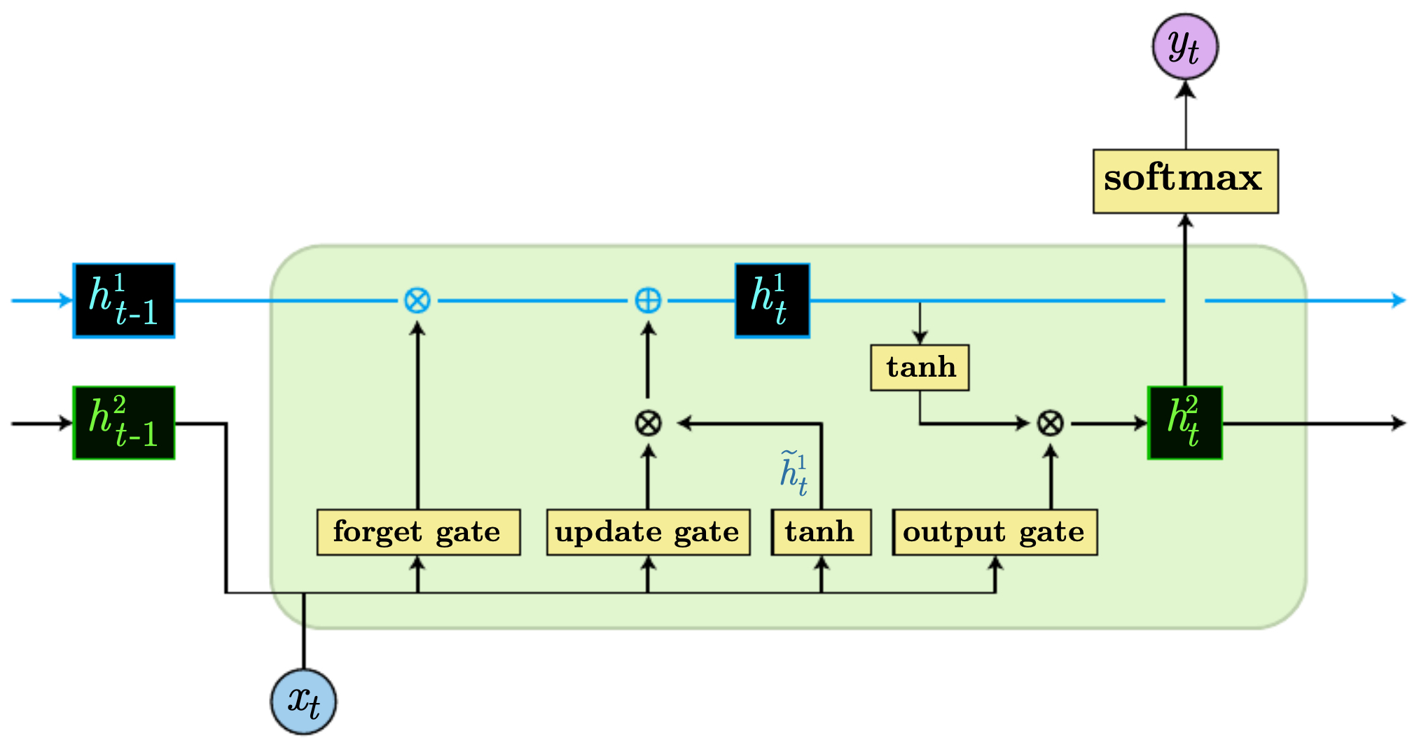
LSTM computational graph
-
The following figure illustrates the internal structure of a single LSTM cell, with the three gates controlling the flow of information into, within, and out of the cell state – the forget, update, and output gates that regulate how memory is stored and exposed across time steps.
-
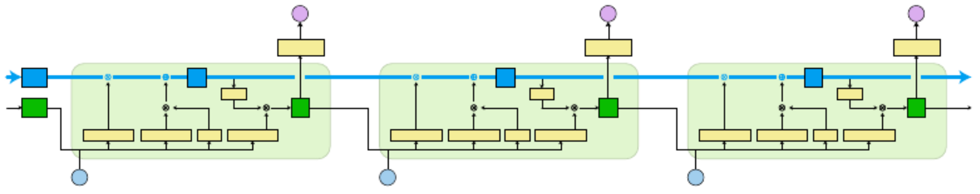
The following figure illustrates stacking multiple LSTM gates in a row.
Why LSTMs capture long-term dependencies
- The key innovation is the cell state \(c^{\langle t\rangle}\), which has an additive update rule:
- Because this update involves elementwise addition (not repeated multiplication as in vanilla RNNs), gradients can flow backward through time more reliably. This makes it possible for the model to learn dependencies spanning hundreds of time steps.
Example: open and close dependencies
- Consider the problem of predicting a closing quotation mark “ ” after a long piece of dialogue. A vanilla RNN would struggle to remember that an opening quotation occurred many steps ago. An LSTM can learn to keep a binary signal in its cell state (via the forget and update gates) that tracks whether a quotation is open, and release this information when the output gate is activated.
Advantages of LSTMs
- Excellent at modeling long-term dependencies.
- More interpretable than GRUs because of explicit memory cell.
- Still widely used in speech recognition, machine translation, and time-series forecasting.
Limitations
- More parameters than GRUs \(\rightarrow\) heavier computation and risk of overfitting.
- Slower training compared to GRUs.
- In modern NLP, largely supplanted by transformers, though still competitive for smaller-scale or low-latency tasks.
Bidirectional recurrent neural networks (BRNNs)
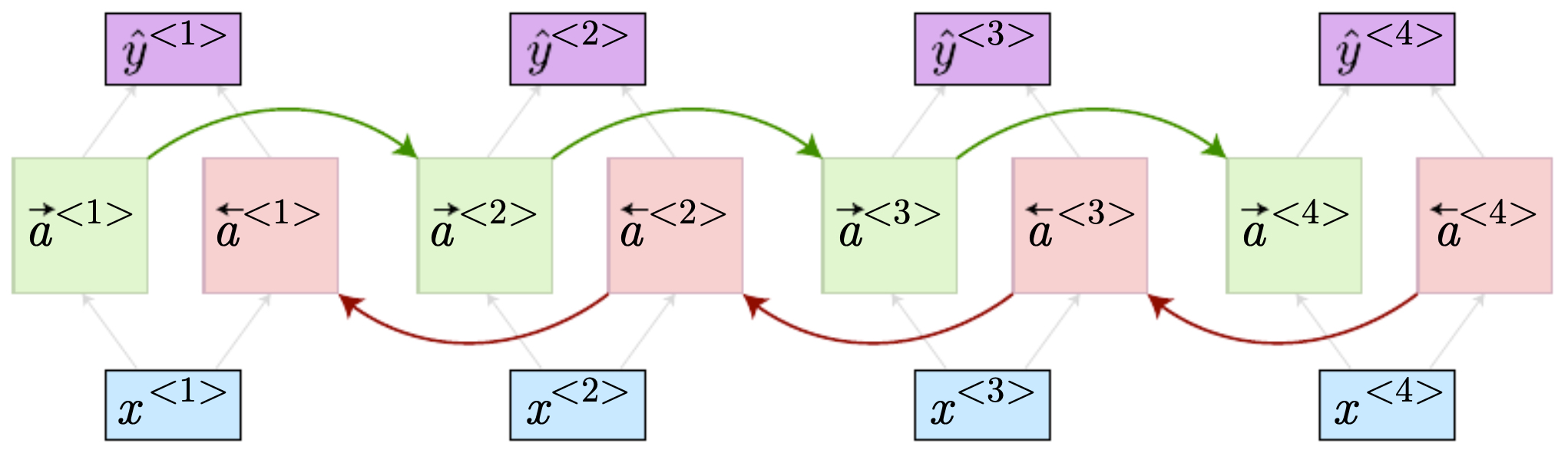
- So far, we have considered RNNs that process sequences in a single direction: left-to-right. However, many tasks require knowledge not only of the past but also of the future context to make accurate predictions. Bidirectional recurrent neural networks (BRNNs) address this by running two RNNs in parallel: one forward and one backward, and then combining their hidden states.
Motivation
-
Consider the sentences:
- “He said, Teddy Roosevelt was a great President.”
- “He said, Teddy bears are on sale!”
-
In both cases, the prefix “He said, Teddy …” is identical. To know whether “Teddy” is a person’s name or a common noun, we need to look not only at the previous words but also at what follows. A unidirectional RNN cannot leverage this future information, but a BRNN can.
Architecture
-
In a BRNN, two hidden states are computed at each time step:
- Forward state \(\overrightarrow{a}^{\langle t\rangle}\) processes the sequence left-to-right.
- Backward state \(\overleftarrow{a}^{\langle t\rangle}\) processes the sequence right-to-left.
-
These are then combined (by concatenation, summation, or another function) to produce the final hidden state:
- The prediction at time step \(t\) is then:
Computation flow
-
Run the forward RNN over the sequence: \(\overrightarrow{a}^{\langle 1\rangle}, \dots, \overrightarrow{a}^{\langle T_x\rangle}\).
-
Run the backward RNN over the sequence in reverse: \(\overleftarrow{a}^{\langle T_x\rangle}, \dots, \overleftarrow{a}^{\langle 1\rangle}\).
-
At each step \(t\), combine \(\overrightarrow{a}^{\langle t\rangle}\) and \(\overleftarrow{a}^{\langle t\rangle}\).
- This design allows predictions at each position to leverage both preceding and following tokens.
Example: Named entity recognition
-
Take the sentence:
-
“He said, Teddy Roosevelt!”
-
At position \(t\) = “Teddy”:
- Forward RNN has context
{He, said, Teddy}`. - Backward RNN has context
{Roosevelt, !}`. - By combining both, the BRNN can correctly infer that “Teddy” refers to a person.
- Forward RNN has context
BRNN diagram
- The following figure shows the structure of a BRNN with an input of length 4. It highlights forward and backward hidden states and how they are combined to form predictions. Each token is represented by two hidden states: one capturing left context and one capturing right context, which are then combined for prediction.
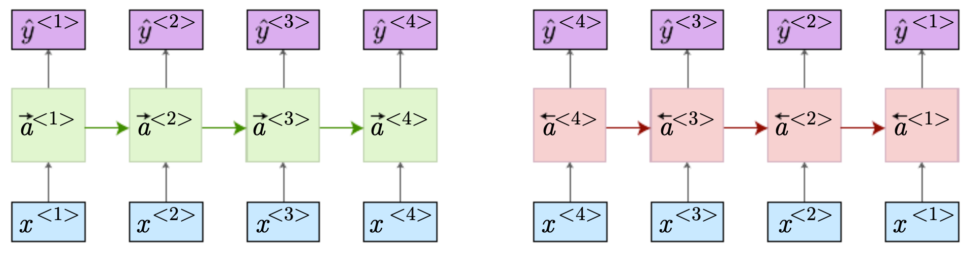
- The following figure shows (left) forward RNN connection with the sequence in order and (right) forward RNN connection, where the sequence is in reverse order.
Advantages of BRNNs
- Use both past and future context \(\rightarrow\) much higher accuracy in per-token predictions.
-
Widely used in tasks such as:
- Part-of-speech tagging
- Named entity recognition
- Speech recognition
- Protein sequence analysis
Limitations
-
Require access to the entire sequence before making predictions.
- Not suitable for real-time streaming tasks (e.g., online speech recognition).
-
Doubles the computation compared to a unidirectional RNN.
Deep recurrent neural networks (Deep RNNs)
- So far, our sequence models have used a single recurrent layer, where each hidden state directly maps to predictions. However, just as stacking layers in feedforward or convolutional networks allows richer representations, we can also stack multiple recurrent layers. These deeper RNNs can capture increasingly abstract temporal patterns and hierarchical dependencies.
Motivation
-
Natural language, speech, and other sequential data often exhibit structure at multiple timescales:
- Lower layers capture short-range features, such as phonemes in speech or character-level patterns in text.
- Higher layers capture long-range and abstract features, such as words, syntactic structures, or sentence-level semantics.
-
By stacking RNN layers, each layer can operate at a different level of abstraction, passing processed information upward.
Architecture
-
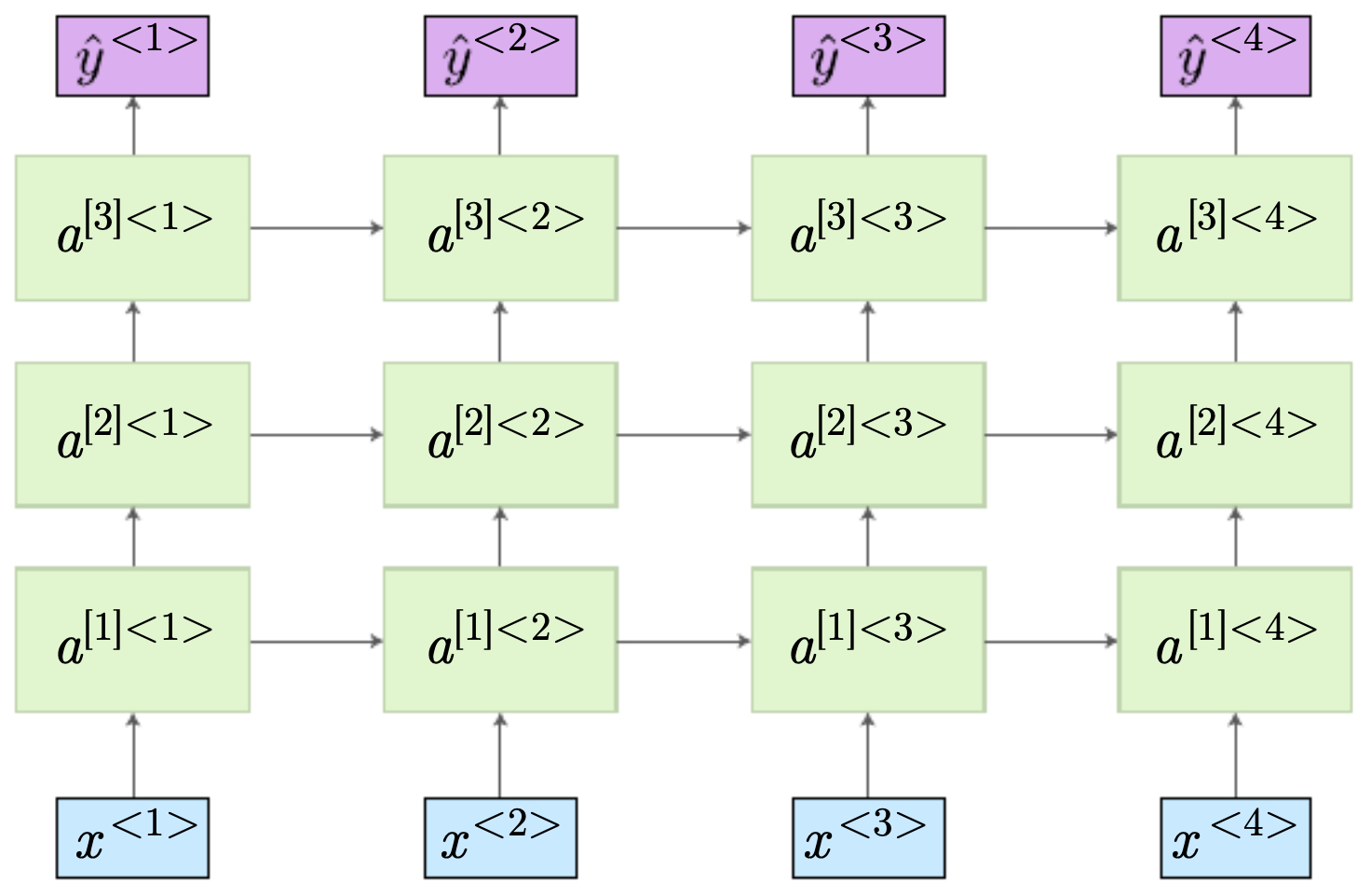
In a deep RNN, the hidden state at layer \(\ell\) and time \(t\), denoted \(a^{[\ell]\langle t\rangle}\), is computed as:
\[a^{[\ell]\langle t\rangle} = g\!\left(W^{[\ell]} \,[a^{[\ell]\langle t-1\rangle}, \ a^{[\ell-1]\langle t\rangle}] + b^{[\ell]}\right)\]-
where:
- \(\ell = 1\) is the first recurrent layer, taking input \(x^{\langle t\rangle}\),
- \(\ell > 1\) layers take input from the previous layer’s hidden state at the same time step,
- Predictions may be taken from the top layer or from intermediate layers.
-
Two main types of deep RNNs
-
Fully stacked recurrent layers Each layer passes activations to both the next time step and the next layer.
- Rich hierarchical temporal modeling.
- Computationally expensive, since each layer propagates across time and depth.
-
Time-restricted deep layers Lower layers propagate across time, while deeper layers only connect within a single time step.
- Reduces computational cost.
- Lets deeper layers focus on abstraction at the current time step.
Diagrams
-
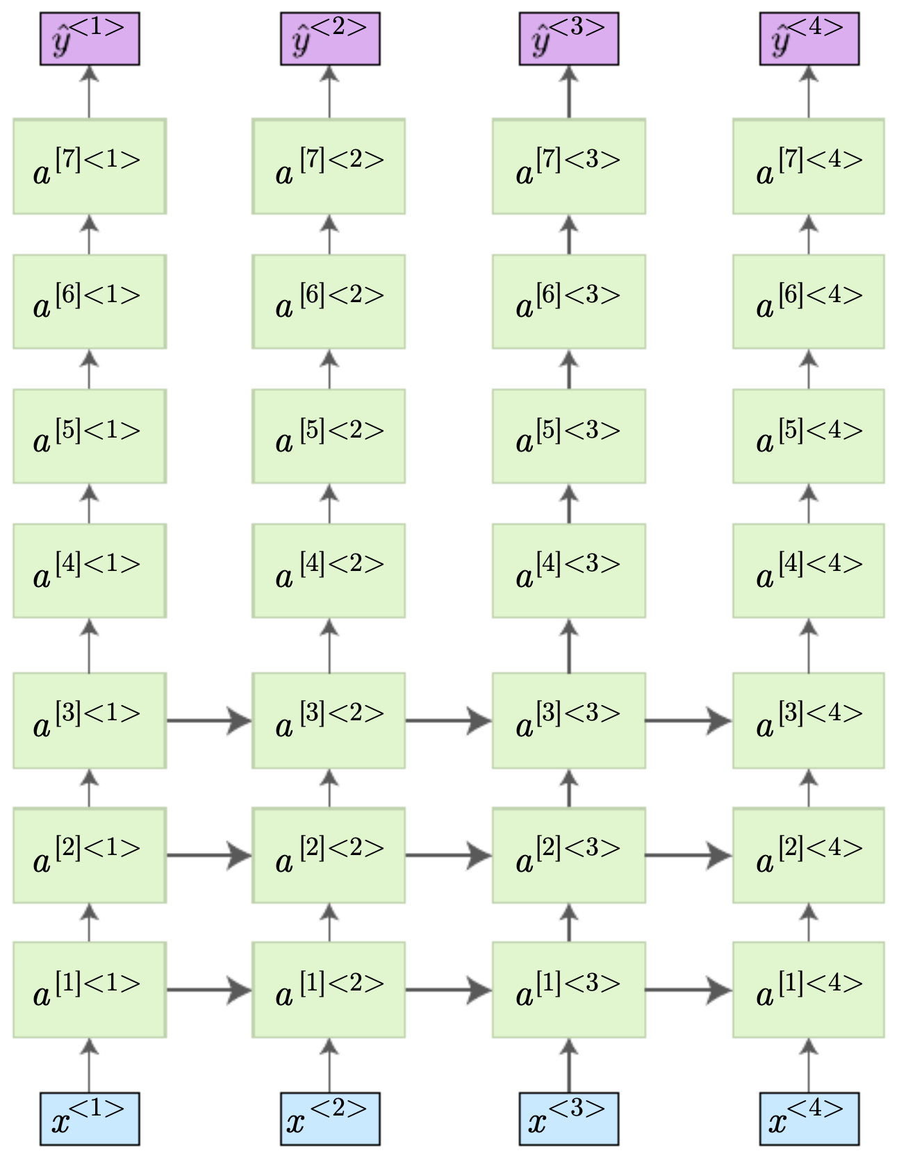
The following figure shows the two primary architectures:
- Stacked deep RNN: multiple layers of recurrence at each time step, each connected forward in time.
- Partially deep RNN: deeper layers exist, but only the lower layers connect across time.
-
The following figure illustrates deep RNN architectures. (Left) Multiple layers of recurrent activations are stacked at each time step and connected through time. (Bottom) Only the first few layers connect across time, while deeper layers connect within a single step.
Advantages of deep RNNs
- Capture hierarchical sequence representations.
- Better at modeling complex temporal dependencies.
- Can reuse features across layers, similar to deep CNNs.
Limitations
- Training is even more prone to vanishing/exploding gradients.
- Computationally heavy: deeper layers multiply the time cost.
- Risk of overfitting on smaller datasets.
Applications
- Speech recognition: lower layers capture acoustic features; higher layers capture words.
- NLP: lower layers encode morphology; higher layers capture syntax and semantics.
- Time series: hierarchical feature extraction across short-term and long-term horizons.
Word embeddings and word representations
- Up until now, we have assumed that words are represented using one-hot vectors. While simple, this representation suffers from serious limitations. To make sequence models effective, we must move toward dense, distributed representations known as word embeddings. These embeddings capture semantic and syntactic relationships among words and form the foundation of modern NLP.
Limitations of one-hot encoding
- Suppose we have a vocabulary of size \(V = 50,000\). A one-hot vector for a word is:
Problems:
- High dimensionality: Each word is represented by a sparse vector of size \(V\).
- No semantics: All words are equidistant—“king” and “queen” are as unrelated as “king” and “banana.”
-
Poor generalization: If the model learns about “orange juice,” it cannot infer anything about “apple juice,” since “orange” and “apple” have no relationship in one-hot space.
- This motivates distributed word representations.
Distributed word embeddings
-
Word embeddings map each word to a dense vector in a lower-dimensional space (typically 100–300 dimensions). Each embedding encodes multiple latent features, such as “royalty,” “gender,” “fruit,” or “color.”
-
For example:
| Word | Royal | Gender | Fruit | Color |
|---|---|---|---|---|
| King | 0.93 | 0.71 | -0.01 | 0.00 |
| Queen | 0.95 | 0.72 | -0.03 | 0.01 |
| Apple | -0.01 | 0.02 | 0.95 | 0.10 |
| Orange | 0.00 | -0.02 | 0.97 | 0.96 |
- Each word is represented as a dense feature vector, allowing the model to reason about similarities and differences.
Transfer learning with embeddings
-
Instead of training embeddings from scratch on small datasets, we can leverage pretrained embeddings trained on billions of words (e.g., Google News, Wikipedia). Common pretrained embeddings include:
- word2vec (Mikolov et al., 2013)
- GloVe (Pennington et al., 2014)
- fastText (Bojanowski et al., 2017)
-
These embeddings can be transferred to smaller tasks (e.g., sentiment analysis, NER), either fixed or fine-tuned.
Properties of embeddings
-
Embeddings capture linear relationships between words:
-
Semantic analogy:
\[\text{vec}(\text{King}) - \text{vec}(\text{Man}) + \text{vec}(\text{Woman}) \approx \text{vec}(\text{Queen})\] -
Similar words cluster in embedding space (e.g., “cat” and “dog”).
-
Embeddings capture nuanced relationships like singular vs. plural, verb tense, and gender.
Comparing embeddings: example
- Suppose our embedding space encodes color and food dimensions. Comparing “apple” and “orange”:
| Feature | Apple | Orange | Apple – Orange |
|---|---|---|---|
| Fruit | 0.95 | 0.97 | 0.00 |
| Orange-colored | 0.00 | 0.98 | -0.98 |
| Royal | -0.01 | 0.00 | -0.01 |
- The difference vector highlights the distinguishing feature (color), while similarities (fruit) are preserved.
Why embeddings matter for sequence models
- Provide dense, information-rich inputs instead of sparse one-hots.
- Facilitate generalization: knowing “orange juice” makes “apple juice” more likely.
- Enable transfer learning, reducing data requirements.
- Serve as the basis for contextual embeddings (ELMo, BERT), which capture meaning in context.
Learning word embeddings
- Word embeddings are not hand-designed; they are learned from large text corpora in a way that captures semantic and syntactic relationships between words. Two of the most influential families of methods are word2vec and GloVe, with later improvements such as fastText. These methods rely on the principle of distributional semantics: a word is known by the company it keeps.
Distributional hypothesis
-
The intuition is simple: words that occur in similar contexts tend to have similar meanings.
-
Example: “The cat drank the …” and “The dog drank the …” \(\rightarrow\) The contexts suggest “cat” and “dog” are semantically related.
-
Embedding learning methods operationalize this by predicting co-occurrence statistics of words and contexts.
word2vec: predictive embeddings
- Introduced by Mikolov et al. (2013), word2vec trains embeddings using neural predictive models. Two main architectures exist:
Continuous Bag of Words (CBOW)
- Task: predict the current word from its surrounding context words.
- Given context \(w_{t-2}, w_{t-1}, w_{t+1}, w_{t+2}\), predict target \(w_t\).
- The embeddings are trained to minimize prediction error.
Skip-gram
- Task: predict surrounding words given the current word.
- Given center word \(w_t\), predict context words \(\{w_{t-k}, \dots, w_{t+k}\}\).
-
Works better for smaller datasets and rare words.
- Formally, skip-gram maximizes:
Negative sampling
-
Instead of computing softmax over the entire vocabulary (expensive), word2vec uses negative sampling:
- For each true word–context pair, sample a few “noise” words.
- Train the model to discriminate true pairs from noise.
- Greatly accelerates training.
GloVe: count-based embeddings
-
GloVe (Pennington et al., 2014) takes a different approach:
- Build a global co-occurrence matrix: counts of how often word \(i\) appears near word \(j\).
- Train embeddings so that their dot products approximate log co-occurrence probabilities.
-
Objective function:
\[J = \sum_{i,j=1}^V f(X_{ij})\left(w_i^\top \tilde{w}_j + b_i + \tilde{b}_j - \log X_{ij}\right)^2\]- where \(X_{ij}\) is the co-occurrence count, and \(f(\cdot)\) is a weighting function.
- Key insight: ratios of co-occurrence probabilities capture semantic relationships.
- For example, the ratio \(P(\text{ice} \mid \text{solid}) / P(\text{steam} \mid \text{solid})\) distinguishes meanings of “ice” vs. “steam.”
fastText: subword embeddings
-
fastText (Bojanowski et al., 2017) improves upon word2vec by incorporating subword (character n-gram) information:
- Each word is represented as the sum of embeddings of its character n-grams.
- Helps with morphologically rich languages and out-of-vocabulary words.
- Example: “playing” shares subword units with “played,” “player,” improving generalization.
Embedding space properties
-
Embeddings capture linear regularities:
-
Analogies:
\[\text{vec}(\text{King}) - \text{vec}(\text{Man}) + \text{vec}(\text{Woman}) \approx \text{vec}(\text{Queen})\] - Clusters: animals, colors, professions naturally cluster in space.
- Cross-lingual mapping: embeddings trained separately on different languages can be aligned, enabling translation.
Summary
- word2vec: predictive models (skip-gram, CBOW) that learn by predicting context.
- GloVe: count-based model that factorizes co-occurrence statistics.
-
fastText: extends word2vec by modeling subword information.
- These embeddings revolutionized NLP by enabling models to leverage semantic structure in text.
From static to contextual embeddings
-
Static embeddings like word2vec and GloVe provide each word with a single fixed vector, regardless of context. While powerful, this approach has limitations:
- The word bank has the same embedding in river bank and bank account, even though the meanings differ.
- Synonyms may collapse into overly similar vectors.
- Polysemy (multiple meanings of a word) is not resolved.
-
To address this, NLP shifted toward contextual embeddings, where a word’s representation depends on its surrounding words.
Contextual embeddings with RNNs
-
Before transformers, the natural way to add context was through RNN-based language models.
- Each word embedding serves as input to an RNN (vanilla, GRU, or LSTM).
- The hidden state at time step \(t\), \(h^{\langle t\rangle}\), encodes the meaning of the word in context:
-
These context-dependent hidden states replace static embeddings when passed to downstream tasks.
-
Thus, the representation of bank in river bank and bank account will diverge because the preceding and following words shape the hidden state.
Bidirectional language models
-
Unidirectional RNNs only capture left-to-right dependencies. But many tasks (NER, POS tagging) need both past and future context.
-
Bidirectional RNN language models (biRNN-LMs) combine forward and backward RNNs, similar to BRNNs, to generate contextual embeddings that reflect the entire sentence.
-
This idea foreshadows ELMo (Peters et al., 2018), which produced embeddings by combining forward and backward LSTMs trained as language models. ELMo was a breakthrough, showing that deep contextual embeddings dramatically improve performance across tasks.
Contextual embeddings vs. static embeddings
| Feature | Static (word2vec/GloVe) | Contextual (RNN-based LM) |
|---|---|---|
| Representation | One vector per word | Different vector per context |
| Handles polysemy | ✗ | ✓ |
| Captures long-range deps | ✗ | ✓ (to some degree with LSTMs) |
| Adaptability | Fixed after training | Dynamic, shaped by sentence |
Example: resolving ambiguity
-
Sentence 1: He sat by the river bank.
- Contextual embedding of bank shifts toward “geographical” meaning.
-
Sentence 2: She deposited cash at the bank.
- Contextual embedding of bank shifts toward “financial institution.”
-
A static embedding cannot make this distinction, but an RNN-based contextual embedding can.
Sequence-to-sequence contextual modeling
-
Contextual embeddings also underpin sequence-to-sequence (seq2seq) architectures:
- Encoder RNN: reads the input sequence and produces contextual embeddings.
- Decoder RNN: generates the output sequence, conditioned on the encoder’s representation.
-
This framework became the standard for machine translation (e.g., Google’s early neural MT systems), and is still foundational in speech recognition and summarization.
Limitations of RNN-based contextual embeddings
- Sequential bottleneck: RNNs process tokens one at a time, limiting parallelization.
- Long-term dependencies: Even LSTMs/GRUs struggle with very long contexts.
-
Compression bottleneck: Seq2seq encoders often compress entire sequences into a single vector, losing detail.
- These challenges paved the way for attention mechanisms, which allow direct connections between all tokens, and ultimately for transformers, which replaced recurrence with self-attention.
Citation
If you found our work useful, please cite it as:
@article{Chadha2020SequenceModels,
  title   = {Sequence Models},
  author  = {Chadha, Aman},
  journal = {Distilled Notes for Stanford CS230: Deep Learning},
  year    = {2020},
  note    = {\url{https://aman.ai}}
}