CS230 • Optimizing and Structuring Neural Networks

• Full-Cycle Deep Learning Projects
  • The Seven Stages of a Project
  • Choosing a Project
  • Illustrative Examples
  • Practical Considerations and Early Prototyping
• Setting up a Machine Learning Application
  • Splitting Data into Training, Development, and Test Sets
  • Bias, Variance, and Error Analysis
  • Learning Curves
• Regularizing a Neural Network
  • Regularization
  • Why Regularization Reduces Overfitting
  • Dropout Regularization
  • Other Regularization Methods
• Setting Up an Optimization Problem
  • Normalizing Inputs
  • Vanishing and Exploding Gradients
  • Weight Initialization for Deep Neural Networks
  • Gradient Numerical Approximations
  • Gradient Checking
• Optimization Algorithms
  • Mini-Batch Gradient Descent
  • Exponentially Weighted Averages (EWA)
  • Bias Correction for EWA
  • Gradient Descent with Momentum
  • RMSProp
  • Adam Optimization Algorithm
  • Learning Rate Decay
  • Local Optima and Saddle Points
• Hyperparameter Tuning
  • Tuning Process
  • Using an Appropriate Scale
  • Hyperparameter Tuning in Practice: Pandas vs Caviar
• Batch Normalization
  • Normalizing Activations in a Network
  • Fitting Batch Norm in a Neural Network
  • Batch Norm at Test Time
• Multi-class Classification
  • Softmax Regression
  • Worked Example
  • Training a Softmax Classifier
• Practical Aspects of Training Softmax Classifiers
  • Numerical Stability
  • Class Imbalance
  • Calibration of Probabilities
  • Large-Scale Classification
  • Regularization for Multi-class Problems
  • Evaluation Metrics Beyond Accuracy
• Citation

Full-Cycle Deep Learning Projects

• Managing a deep learning project is a multidisciplinary process that requires careful attention across the entire lifecycle, from idea conception to long-term maintenance. While academic literature often focuses narrowly on architectures, training algorithms, and benchmark performance, real-world systems demand a broader perspective.
• As Andrew Ng and others have emphasized in industry (Amodei et al., 2016), the system view is often more critical than model novelty.

The Seven Stages of a Project

• Most projects, regardless of domain, can be divided into seven stages:

  1. Project selection
  2. Data acquisition
  3. Deep learning model design
  4. Model training
  5. Model testing
  6. Deployment
  7. Maintenance

• These stages are not linear but iterative: data issues discovered during testing may require revisiting data acquisition, deployment challenges may necessitate architectural changes, and maintenance often triggers new rounds of retraining. In practice, teams operationalize this by setting explicit “exit criteria” for each stage (e.g., target data coverage at acquisition; minimum offline AUC before training can end; SLOs for deployment). Feedback loops connect adjacent stages: telemetry from deployment feeds maintenance and, in turn, updates data pipelines and retraining schedules. Strong project hygiene also adds cross-cutting tracks—experiment tracking, observability, and risk assessment—that run alongside all seven stages.

Choosing a Project

• A good project balances interest, feasibility, and impact:

  • Interest: Does the project sustain long-term curiosity and motivation?
  • Impact: How will it affect people’s lives or business outcomes?
  • Data: Are sufficient datasets available, or can they be collected at reasonable cost and speed?
  • Domain knowledge: Does the team bring unique expertise to the task?

• Feasibility is often the most subtle and crucial consideration. In practice, feasibility can be evaluated using human-level performance as a reference point. If humans can perform a task reliably under the same input conditions, it is reasonable to expect a neural network can approach or surpass that performance given enough data and tuning. Concretely, teams estimate the “Bayes error” proxy from expert raters, then design milestones (e.g., within 5 percentage points of human accuracy) and data requirements (labeling hours, class balance, operating-condition coverage). Early scoping should also map the decision boundary to the available sensor stack, latency budgets, and privacy/security constraints.

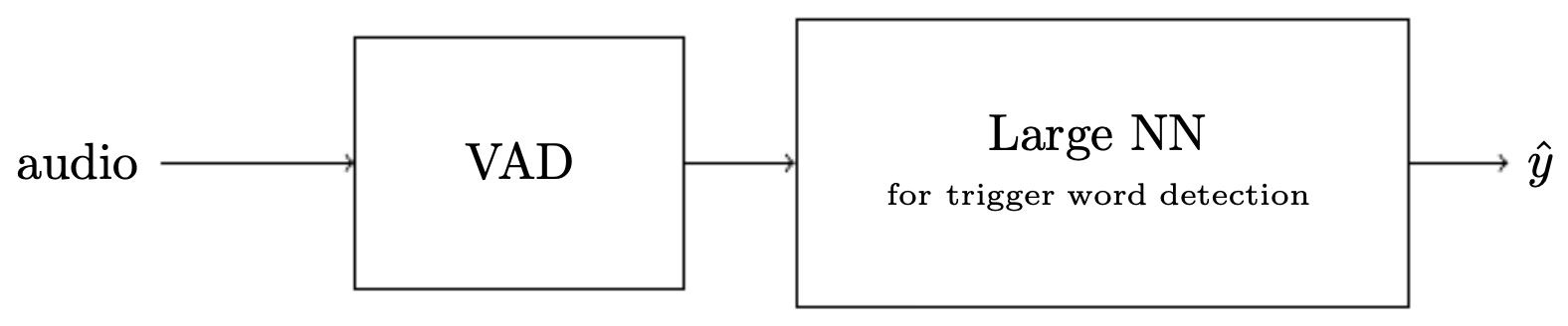
• The following figure illustrates this principle in the context of trigger word detection, where the overall task is decomposed into modular subtasks. Specifically, the trigger word detection problem is decomposed into two stages: voice activity detection (VAD) and trigger word detection, demonstrating modular system design. By isolating VAD, the system filters out non-speech segments cheaply (often with DSP or a tiny NN), dramatically reducing downstream compute and false positives. The trigger detector then operates only on speech frames, where a higher-capacity model can focus on phonetic patterns and temporal alignment. This decomposition clarifies data needs (background noise for VAD; phonetic variability for the trigger) and allows independent evaluation metrics (VAD ROC vs. trigger precision–recall at fixed VAD recall), making the engineering plan measurable and iterative.

Illustrative Examples

• Two canonical examples from industry practice highlight these principles:

  1. Trigger Word Detection (Amazon Alexa, Siri, etc.):

     • Goal: Detect whether a spoken word such as “Alexa” has been uttered.
     • Decomposition: First detect whether speech is present (voice activity detection, VAD), then determine whether the word matches the trigger.
     • Early Prototyping: Even a small dataset of a few hundred samples is enough to start iterating.
     • Additional details: Label design matters (frame-level vs. clip-level); the positive class is sparse, so class-imbalance handling (focal loss, weighted sampling) prevents degenerate solutions. Temporal modeling can start with simple CMVN + MFCCs and evolve to learnable front-ends (conv layers on log-mel spectrograms). Evaluation uses operating-point curves (false accept vs. false reject) at target FARs (e.g., 1 per 24 hours).

  2. Door Lock Face Recognition:

     • Goal: Unlock a door when the system recognizes the registered user’s face.
     • Framing: A binary classification task — given two images, determine if they belong to the same person.
     • Practical Challenge: Starting with a small dataset (collected over a few days) helps quickly identify real-world pitfalls, such as poor performance under different lighting conditions.
     • Additional details: On-device constraints (compute, power) often favor embedding-based verification with a cosine distance threshold. Data collection should explicitly cover pose, illumination, and occlusion (P-I-O). Liveness defenses (blink detection, depth, IR) and privacy considerations (encrypted embeddings, on-device enrollment) shape both architecture and deployment.

• Both examples emphasize a general development philosophy: start simple, iterate fast, and document everything. Concretely, teams maintain a decision log (assumptions, rejected alternatives, metrics changes), an experiment registry (configs, seeds, commits, artifact hashes), and a risk register (data drift, attack surfaces, failure modes), which together make the iteration loop reliable and auditable.

Practical Considerations and Early Prototyping

• Small-scale experiments (few hundred to thousand examples) can expose hidden difficulties such as accent variability in speech or lighting mismatches in vision. Rapid pilots should be end-to-end (data → model → metric) even if crude, because system-level issues (latency, memory footprint, edge cases) surface only in full loops.
• Simple baselines first: For example, non-machine-learning heuristics for VAD (e.g., amplitude thresholds) or activity detection (e.g., frame differencing for motion detection at a door) often provide robust and energy-efficient baselines before moving to full neural solutions. Baselines set a lower bound and clarify where ML adds value.
• Documentation: Tracking model architectures, hyperparameters, and results across iterations ensures reproducibility and facilitates error analysis later. Couple this with dataset versioning (immutability, provenance, schema checks) and evaluation contracts (frozen dev/test splits, stable metrics) so that improvement claims are meaningful.
• This prototype-first, optimize-later philosophy is consistent with agile methods and avoids premature optimization. As pilots mature, promote artifacts into production-grade components: data validation (schema, anomaly detection), training pipelines (idempotent, distributed), CI for models (unit tests for data transforms, gradient checks, numerical determinism), and monitoring (input drift, performance decay, alerting tied to SLOs).

Setting up a Machine Learning Application

• Once a project has been selected, the next step is to set up the machine learning pipeline: partitioning data, establishing metrics, and preparing the system for robust training and evaluation. This stage lays the groundwork for the entire lifecycle: bad data splits or poorly chosen metrics can invalidate downstream results, while thoughtful setup accelerates iteration and reduces surprises in deployment.

Splitting Data into Training, Development, and Test Sets

• Deep learning practice requires dividing data into subsets that serve different purposes:

  • Training set: used to fit model parameters. It should be representative and large enough to cover the distribution of inputs the model will see in practice.
  • Development (validation) set: used to tune hyperparameters and make design choices. This set serves as the “proxy for production” during experimentation.
  • Test set: used only at the end, to provide an unbiased estimate of performance. It should never influence model design.

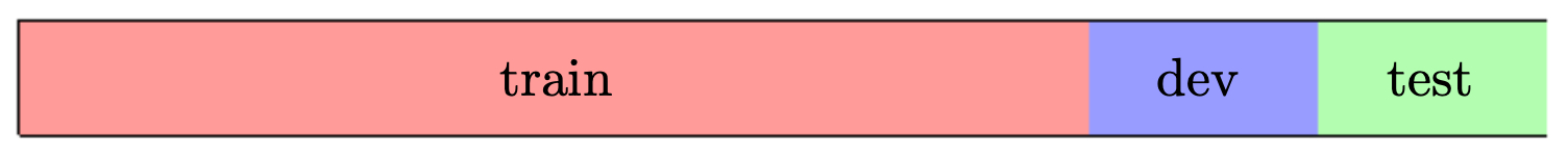
• The following figure illustrates this partitioning process of dividing the available data into training, development, and testing sets. A common split is 80/10/10, but the ratio depends on total dataset size and intended usage. For example, in medical applications with small datasets, a 60/20/20 split may be preferable, while in web-scale settings, holding out even 1% can produce millions of test examples.

• In addition to size, the sampling method matters: splits should reflect the true deployment distribution. Stratified sampling ensures class balance, and temporal splits are crucial when dealing with time-series data (e.g., training on past data, validating on more recent data). For cross-device systems, splitting by user rather than example prevents leakage that would inflate performance estimates.

Bias, Variance, and Error Analysis

• Performance must be diagnosed in terms of bias and variance:

  • High bias (underfitting): The model is too simple to capture underlying patterns.
  • High variance (overfitting): The model performs well on training data but poorly on unseen data.
  • Balanced tradeoff: Ideally, both bias and variance are low.

• Error analysis, guided by these categories, helps determine whether the next step should be more data, more regularization, or a different architecture. For instance, high training and dev error together suggest the need for a more expressive model or better features; low training error but high dev error suggests adding data, regularization, or improved augmentation.

Learning Curves

• Learning curves are a practical diagnostic tool. By plotting training and development error as a function of training set size, one can identify whether a model is limited by bias or variance.

  • If both training and dev error are high → high bias (underfitting).
  • If training error is low but dev error is high → high variance (overfitting).
  • If both are low → good fit.

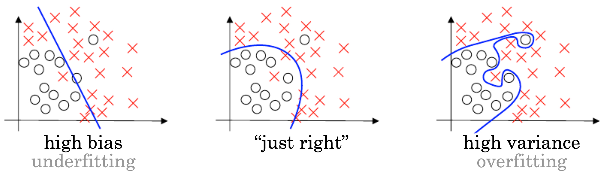
• The following figure illustrates the bias–variance tradeoff in machine learning models. It shows how bias and variance errors affect model performance, with underfitting and overfitting representing opposite ends of the spectrum.

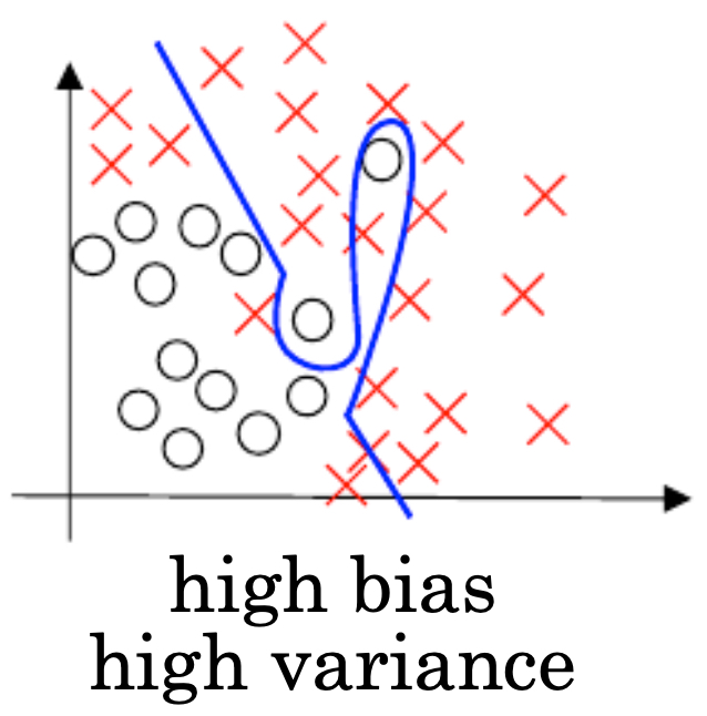
• The following figure shows an example of a model having both high variance and high bias — an unfavorable situation where the model is both too simplistic in parts and overfitted in others, often due to poor feature representation or noisy labels.

• In practice, bias–variance decomposition is complemented by granular error analysis: inspecting confusion matrices, segmenting errors by input type (e.g., accent groups in speech recognition), or plotting performance by confidence scores. This layered view helps distinguish whether failures stem from model capacity, data scarcity, label quality, or distribution shift.

Regularizing a Neural Network

• When training deep networks, a common challenge is overfitting, where the model performs well on training data but poorly on unseen data. Regularization introduces constraints or noise to prevent overfitting and improve generalization. In practice, a mix of regularization techniques is often used, tailored to the data scale, model capacity, and deployment constraints.

Regularization

• Consider logistic regression with a cost function:

• Adding an L2 regularization term yields:

• This modification penalizes large weights, effectively discouraging overly complex models. L1 regularization is another option, which encourages sparsity by pushing weights toward exactly zero. In practice, L2 is favored for stability, while L1 is used when interpretability or feature selection is desired.

• For multi-layer networks, the regularized cost function generalizes to:

• Here, the Frobenius norm penalizes the magnitude of the entire weight matrix at each layer. Regularization can thus be seen as injecting prior knowledge — a preference for simpler, smoother hypotheses.

Why Regularization Reduces Overfitting

• If the weights connected to a neuron are very small, the neuron’s contribution is negligible, simplifying the model. By limiting effective degrees of freedom, regularization forces the network to learn only the strongest, most generalizable patterns rather than memorizing noise.

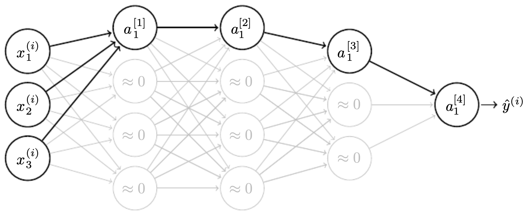
• The following figure shows how reducing the magnitude of weights diminishes the influence of a neuron, effectively simplifying the hypothesis class and reducing overfitting risk. In this view, regularization acts like “weight shrinkage,” pulling neurons back toward inactivity unless they consistently improve prediction.

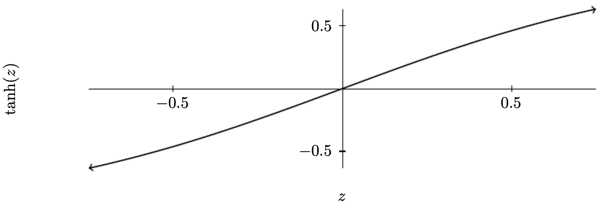
• When weights shrink, activations often become linear, reducing model complexity. For example, the hyperbolic tangent behaves nearly linearly around zero. If most inputs fall in this nearly linear region, the network is less able to overfit fine-grained noise.

• The following figure illustrates how the hyperbolic tangent function is nearly linear around the origin, making it less expressive when weights are small. This explains why L2-regularized networks often appear more stable during training — they operate in low-curvature regimes of activation functions.

Dropout Regularization

• Dropout is another widely used technique: during training, hidden neurons are randomly removed with some probability, forcing the network not to rely too heavily on any single feature (Srivastava et al., 2014).

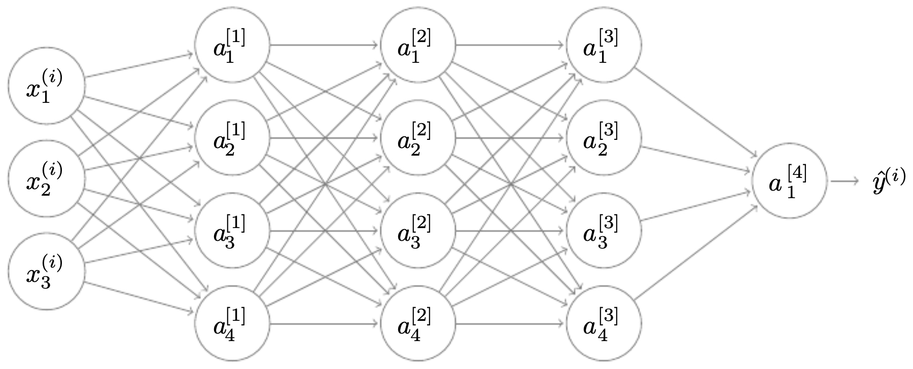
• The following figure shows a fully connected 4-layer neural network before dropout is applied, where all neurons are active. Such dense connectivity risks strong co-adaptation: neurons may form fragile, overly specific feature detectors.

• During dropout, some neurons are removed, leaving only a subset active. This forces the network to distribute learning across redundant pathways.

• The following figure illustrates the same neural network after dropout, where several hidden neurons are removed. Training on these thinned networks ensures robustness: at test time, when all neurons are reactivated, the network behaves like an ensemble of its dropout-trained subnetworks.

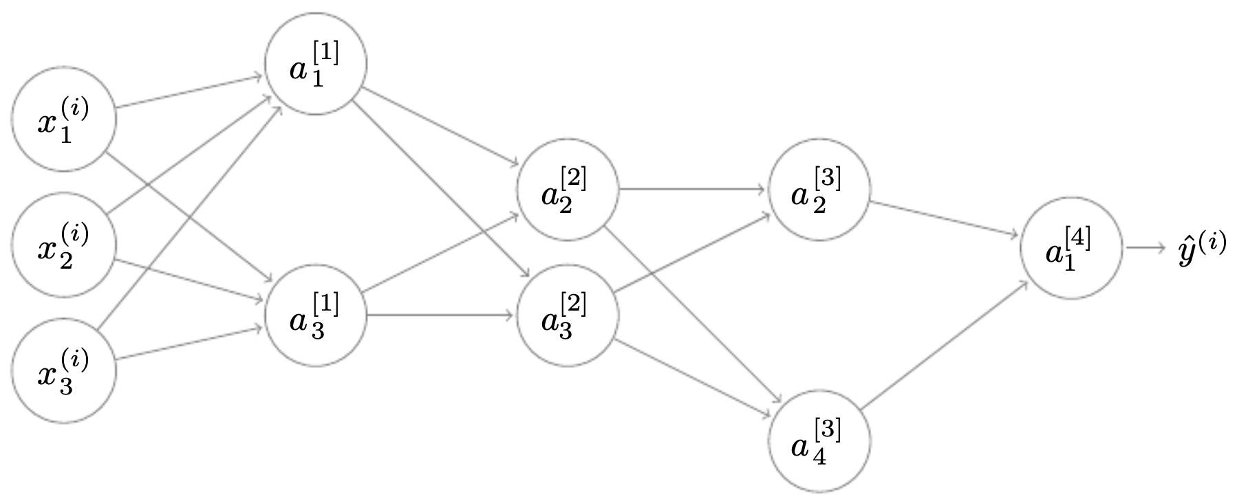
• At inference, all neurons are used, but their outputs are scaled (by the dropout rate) to match expected activations during training. This scaling rule prevents distribution shift between train and test time.

Other Regularization Methods

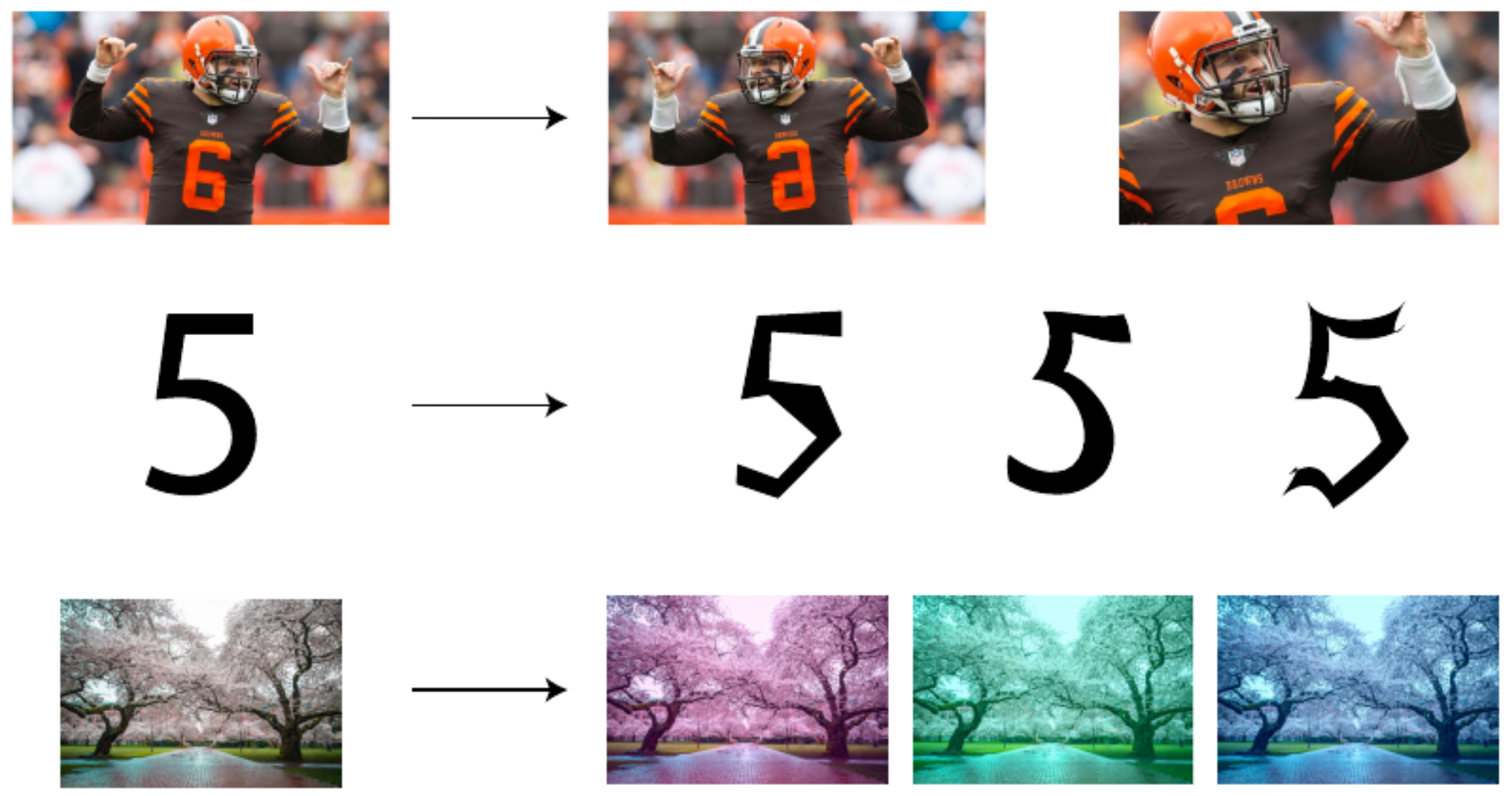
• When new data is unavailable, data augmentation artificially increases training diversity. For images, this can involve rotations, crops, flips, brightness/contrast changes, and even adversarial perturbations. Augmentation reduces overfitting by exposing the model to more varied input distributions, simulating how real-world data may differ from training examples.

• The following figure demonstrates examples of data augmentation techniques such as rotation, translation, and color perturbations applied to image inputs. These transformations preserve labels while forcing the model to generalize across nuisance variability.

• Another method is early stopping, where training halts before overfitting occurs, trading off full convergence for generalization. By monitoring validation error, training can be cut off once error begins to rise, preventing the model from memorizing noise in the training set.

• Collectively, these methods form a toolbox: weight regularization enforces simplicity, dropout enforces redundancy, data augmentation enforces invariance, and early stopping enforces restraint. Together, they are essential for making deep networks work in practice.

Setting Up an Optimization Problem

• Optimization is at the heart of training neural networks. While model architecture determines representational capacity, optimization governs whether that capacity is realized in practice. Poor optimization can lead to extremely slow convergence, exploding or vanishing gradients, or convergence to poor local regions. Good optimization practices, on the other hand, stabilize learning, accelerate training, and often improve generalization.

Normalizing Inputs

• One of the simplest yet most powerful practices is normalizing inputs. Neural networks train faster and more reliably when the input features are centered around zero and have unit variance.

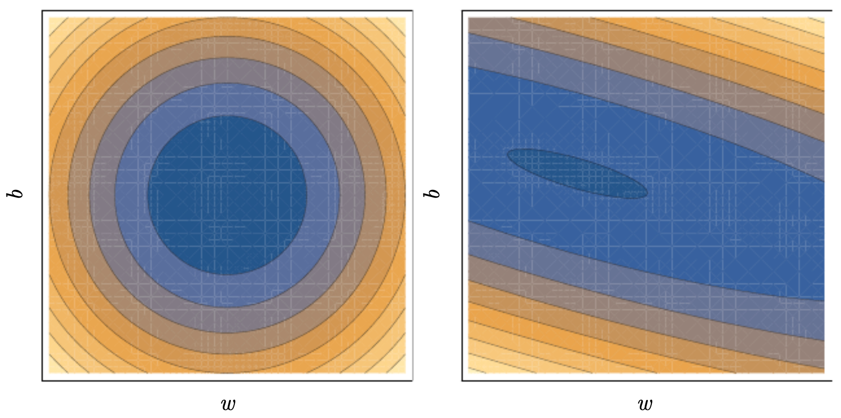
• Suppose we have raw input features with arbitrary ranges. If feature 1 ranges from 0 to 1 but feature 2 ranges from 0 to 1000, gradient descent will zigzag inefficiently because the cost function contours are elongated ellipses. Normalization makes the contours more circular, allowing gradient descent to take balanced steps in all directions.

• Step 1: Centering the mean. Subtract the mean of each feature so that it is centered at 0.

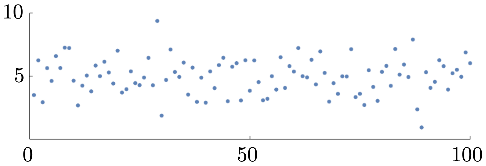
• The following figure shows the original distribution of features before normalization, with mean centered at 5 and variance 2.25.

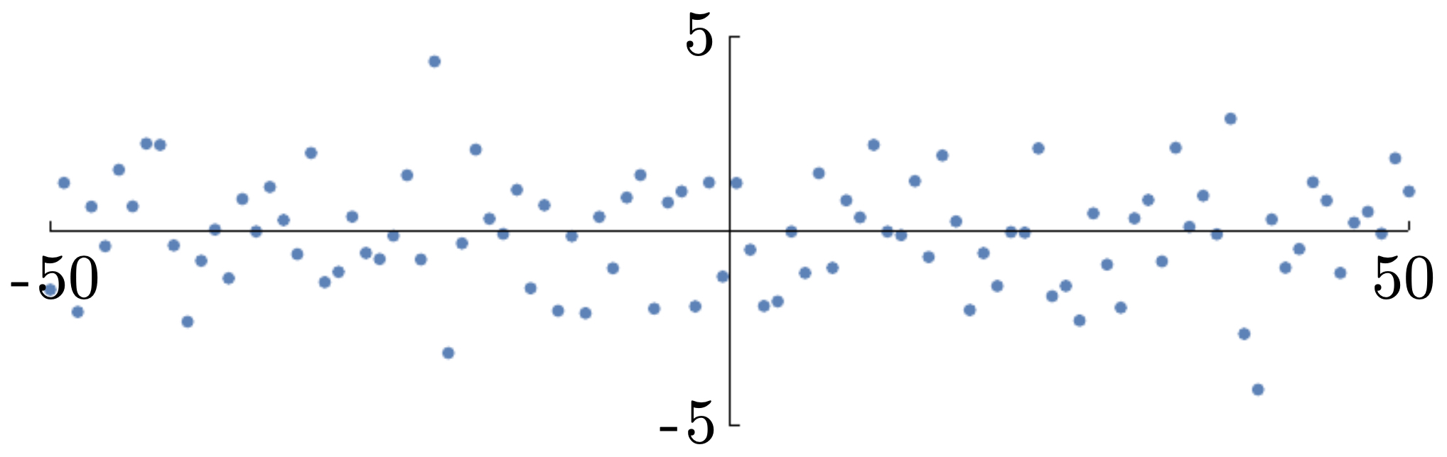
• Step 2: Shifting mean to 0.

• The following figure illustrates the same dataset after centering, shifting the mean to 0.

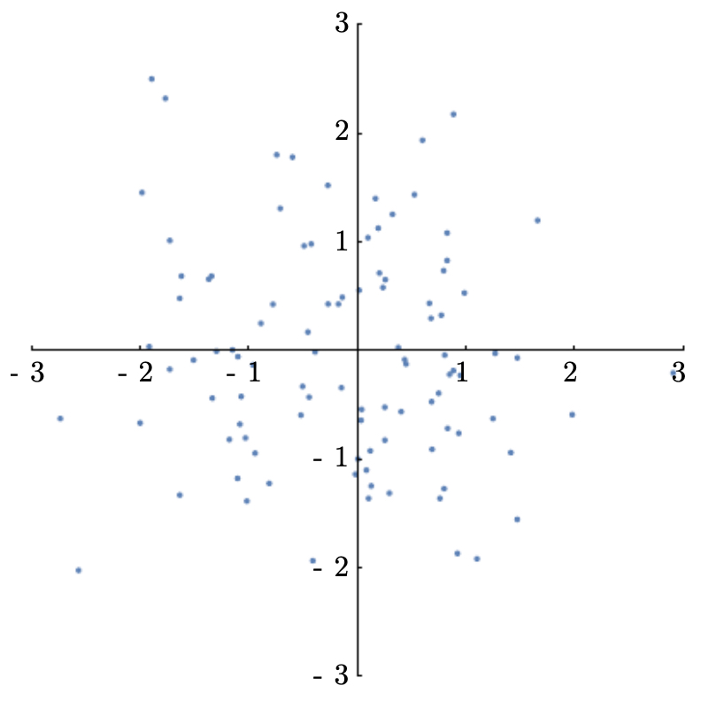
• Step 3: Scaling to unit variance. Divide by the standard deviation so that variance is 1.

• The following figure shows the dataset after scaling variance to 1, completing the normalization process.

• Normalization not only makes optimization smoother, but also reduces sensitivity to hyperparameters like learning rate.

• The following figure compares contour plots for gradient descent on unnormalized vs. normalized data, demonstrating that normalization creates more circular contours and accelerates convergence.

Vanishing and Exploding Gradients

• Deep networks can suffer from vanishing or exploding gradients. This problem arises because gradients are propagated through many layers, each multiplication by a weight matrix potentially shrinking or amplifying values.

• If weights are initialized too small (<1), gradients shrink exponentially with depth, causing early layers to learn extremely slowly (vanishing). If weights are too large (>1), gradients grow exponentially, destabilizing training (exploding).

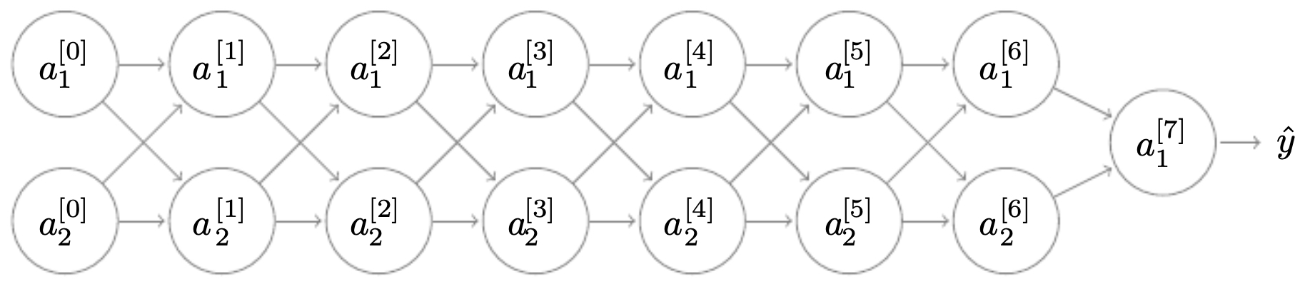
• The following figure illustrates a 7-layer neural network, where signal propagation across many layers can lead to vanishing or exploding gradients if initialization is poorly chosen.

Weight Initialization for Deep Neural Networks

• To combat these issues, careful weight initialization strategies are used:

  • Xavier initialization (Glorot & Bengio, 2010) for activations like tanh:
  \[\sigma^2 = \frac{1}{n^{[\ell-1]}}\]
  • He initialization (He et al., 2015) for ReLU activations:
  \[\sigma^2 = \frac{2}{n^{[\ell-1]}}\]

• These formulas balance the variance of activations across layers, preventing exponential growth or decay.

Gradient Numerical Approximations

• Numerical gradient checks are a practical debugging tool. Instead of trusting backprop blindly, we can approximate derivatives via finite differences and compare them with analytical gradients.

• One-sided limit:

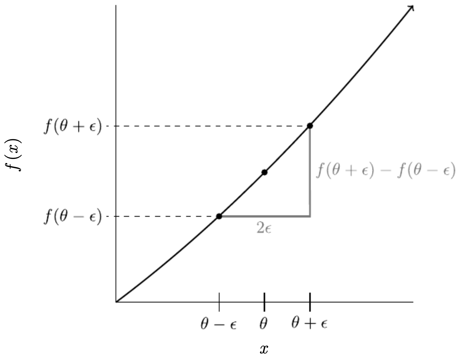
• Two-sided limit (preferred for accuracy):

• The following figure visualizes the two-sided derivative approximation using finite differences.

Gradient Checking

• Gradient checking compares backpropagated derivatives with numerical approximations to catch bugs in implementation.

• Key points:

  • Include regularization terms in both analytical and numerical gradients.
  • Do not use dropout during gradient checking, since randomness breaks determinism.
  • Small discrepancies are expected due to floating-point precision, but large mismatches indicate a bug.

Optimization Algorithms

• Once inputs are normalized and weights are properly initialized, the choice of optimization algorithm determines how efficiently a neural network converges. Gradient descent is the foundation, but many variants improve stability, speed, and robustness. The algorithms differ in how they update parameters using gradients, past information, and adaptive learning rates.

Mini-Batch Gradient Descent

• The simplest method is batch gradient descent, which computes the gradient using the entire training set at each step. While accurate, it is computationally expensive for large datasets.

• At the other extreme, stochastic gradient descent (SGD) uses a single training example per step, which is noisy but fast.

• Mini-batch gradient descent balances both worlds: it computes gradients on small batches (e.g., 32–512 samples). This reduces variance in updates, allows efficient use of GPU parallelism, and accelerates convergence.

• The following figure compares the cost progression for batch gradient descent (smooth convergence) and mini-batch gradient descent (noisier, but faster).

• Mini-batch size is a hyperparameter:

  • Mini-batch = \(m \;\Rightarrow\;\) batch gradient descent.
  • Mini-batch = \(1 \;\Rightarrow\;\) stochastic gradient descent.
  • Intermediate sizes \(\;\Rightarrow\;\) practical compromise.

Exponentially Weighted Averages (EWA)

• Mini-batch gradient descent can still be noisy. To smooth signals, we use exponentially weighted averages (EWA). This technique weighs recent gradients more heavily than older ones, effectively providing momentum-like smoothing.

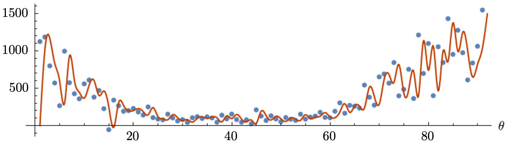
• The following figure shows the raw dataset that exponential smoothing will be applied to.

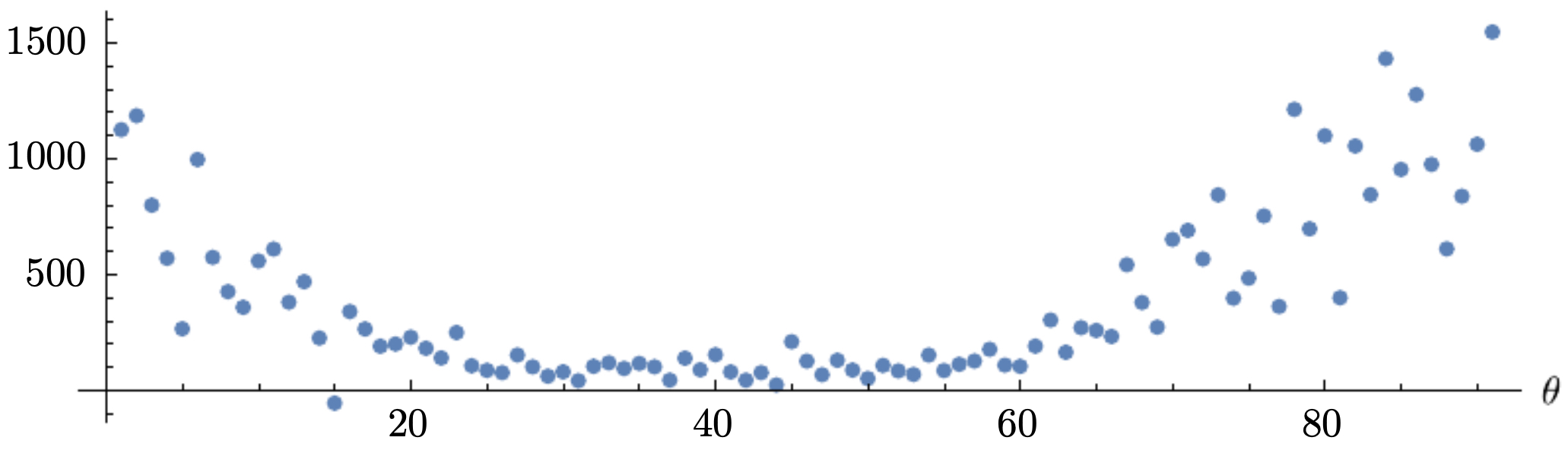
• After applying EWA, the signal becomes smoother, as shown in the next figure (red curve).

• The smoothing degree is controlled by parameter \(\beta\):

  • Small \(\beta\) (e.g., \(\beta = 0.01\)) \(\;\Rightarrow\;\) very responsive but noisy.
  • Large \(\beta\) (e.g., \(\beta = 0.95\)) \(\;\Rightarrow\;\) very smooth but slow to adapt.

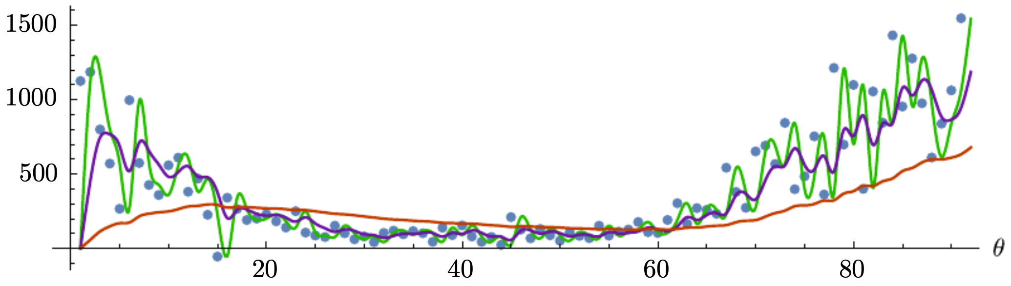
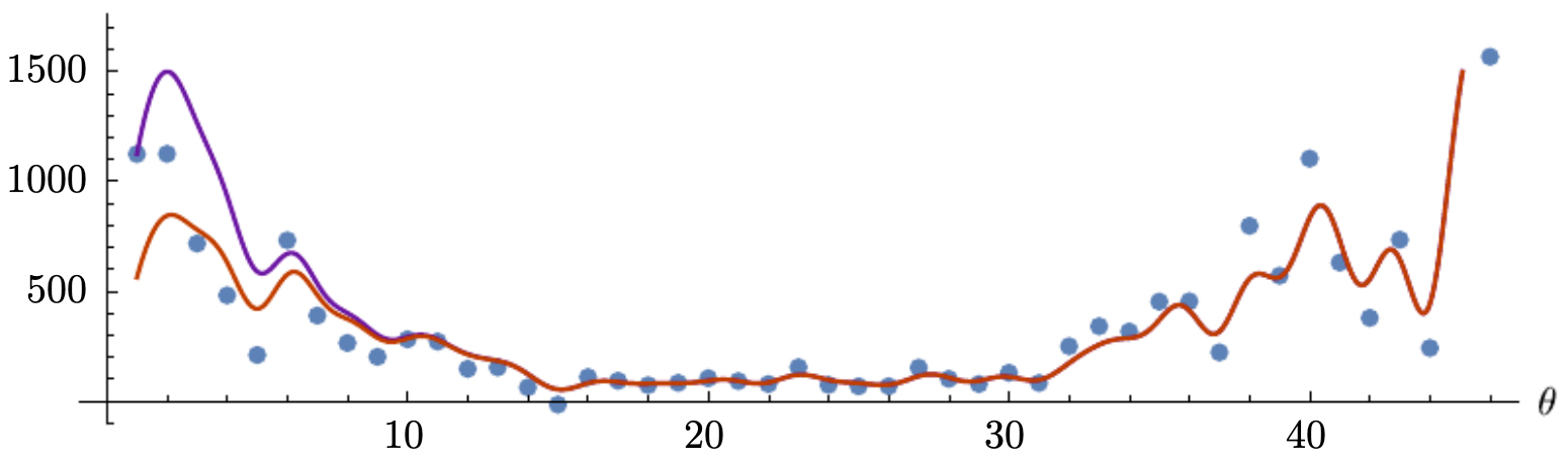
• The following figure demonstrates how different values of \(\beta\) affect smoothness: \(\beta = 0.01\) (green), \(\beta = 0.6\) (purple), \(\beta = 0.95\) (orange).

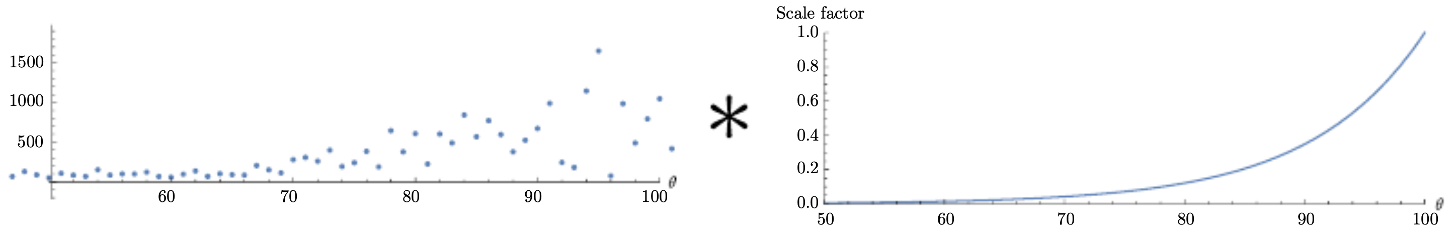
• Another way to interpret EWA is through decay scaling factors, which decrease exponentially over time. The figure below illustrates this.

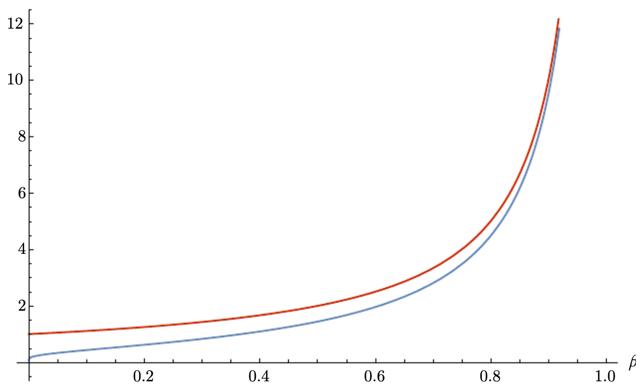
• The effective time window of an EWA is approximately

• The following figure compares this approximation (red) with the real time constant (blue):

Bias Correction for EWA

• At the beginning of training, exponentially weighted averages are biased towards zero because there isn’t enough history.
• Bias correction rescales the averages to remove this underestimation:

• The following figure compares bias-corrected weighted averages (purple) against uncorrected ones (red).

Gradient Descent with Momentum

• Momentum accelerates gradient descent in the right direction and dampens oscillations. Instead of using only the current gradient, we update parameters using an exponentially weighted average of past gradients:

• This allows the optimizer to build “velocity” in consistently good directions, much like a ball rolling down a slope.

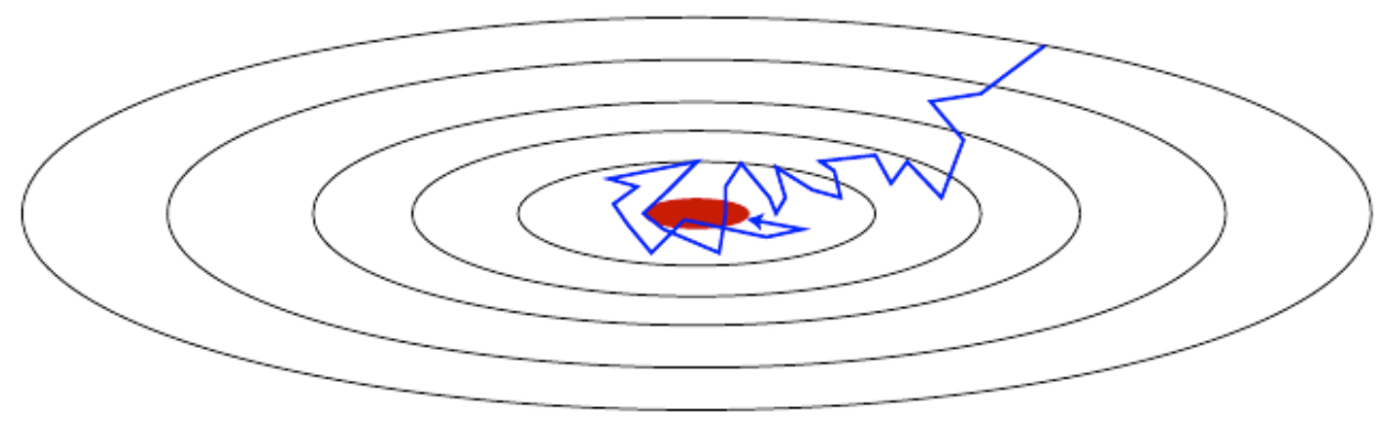
• The following figure shows the contour plot of gradient descent paths with momentum, highlighting smoother and faster convergence compared to plain gradient descent.

RMSProp

• RMSProp rescales gradients by their recent magnitudes, preventing oscillations when different parameters have very different scales.

• Without RMSProp, parameters with large gradient magnitudes dominate the update, causing erratic learning.

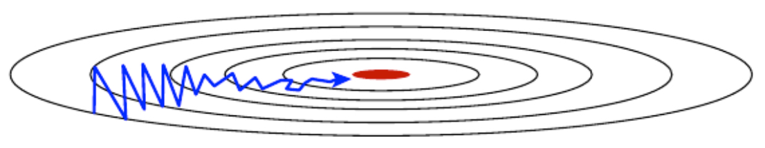
• The following figure illustrates oscillations in gradient descent due to imbalanced gradient magnitudes across parameters.

Adam Optimization Algorithm

• Adam (Kingma & Ba, 2015) combines momentum (exponentially weighted averages of past gradients) and RMSProp (scaling by past squared gradients).

• Update rules:

• Default hyperparameters:

  • \[\beta_1 = 0.9\]
  • \[\beta_2 = 0.999\]
  • \[\epsilon = 10^{-8}\]

Learning Rate Decay

• Even with Adam or momentum, a fixed learning rate can cause problems near minima. Large steps may cause the algorithm to bounce around the optimum instead of converging.

• Learning rate decay gradually reduces the step size:

• or exponentially:

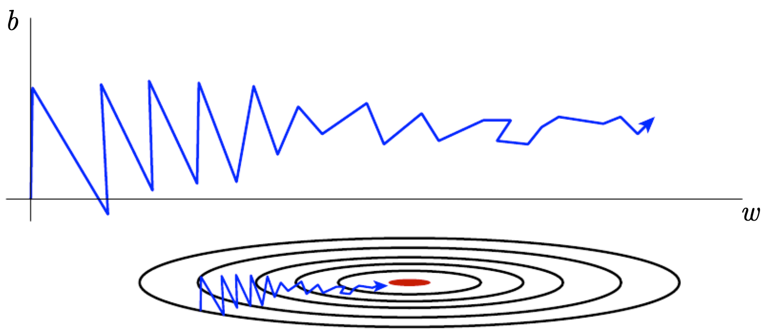
• The following figure shows how gradient descent may bounce around the minimum if learning rate is not decayed.

Local Optima and Saddle Points

• In high-dimensional spaces, local minima are rare. The real challenges are saddle points (where \(\nabla J = 0\) but curvature is mixed) and flat plateaus (where gradients vanish).

• Modern optimization algorithms (momentum, RMSProp, Adam) help escape these regions by maintaining velocity and adaptive scaling.

Hyperparameter Tuning

• Hyperparameter tuning is essential in deep learning, since performance depends strongly on values like learning rate, momentum, number of hidden units, and mini-batch size. The search for good hyperparameters can significantly influence both training efficiency and final accuracy.

Tuning Process

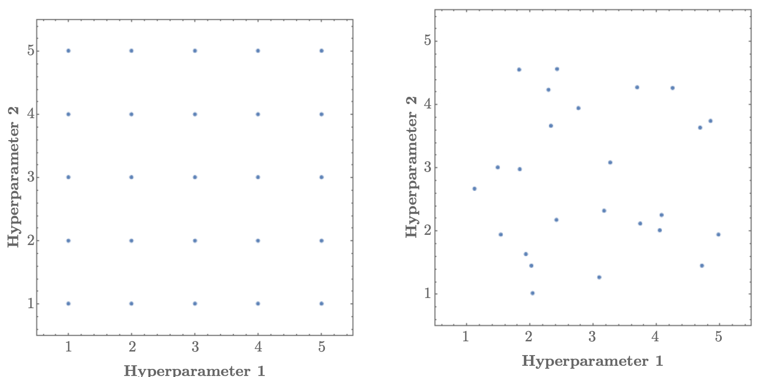
• Hyperparameters should be explored systematically. A naive method is grid search, but in high-dimensional spaces it wastes resources. A more effective approach is random search (Bergstra & Bengio, 2012), since it explores a wider variety of values.

• The following figure compares grid search (left), which samples evenly but inefficiently, with random search (right), which provides better coverage of the hyperparameter space.

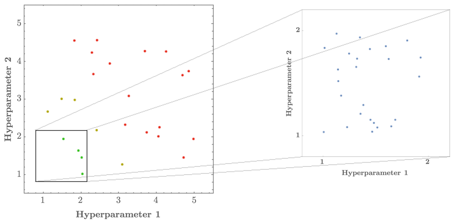
• A coarse-to-fine strategy refines the search. Broad random sampling first identifies promising regions, followed by fine-grained exploration.

• The following figure shows the coarse-to-fine narrowing process, where initial random samples guide subsequent fine-grained search in relevant ranges.

Using an Appropriate Scale

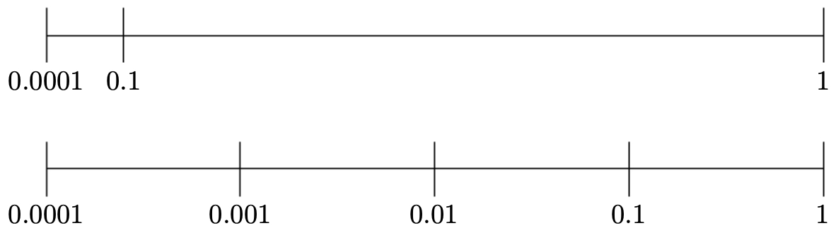
• Some hyperparameters, like learning rate, vary over orders of magnitude. It is better to sample on a logarithmic scale rather than a linear one.

• Example:

  • Instead of drawing \(\alpha \sim \text{Uniform}(0.0001, 1)\),
  • draw \(\log_{10}(\alpha) \sim \text{Uniform}(-4, 0)\).

• The following figure compares linear scale binning (top), which wastes resolution in unimportant regions, with logarithmic scale binning (bottom), which better captures orders of magnitude.

• Similarly, for parameters close to 1 (e.g., momentum terms \(\beta\)), tuning is more effective on \(1 - \beta\) rather than \(\beta\) directly, since small differences near 1 can have large effects.

Hyperparameter Tuning in Practice: Pandas vs Caviar

• Two common philosophies in research and industry:

1. Pandas approach: Carefully adjust hyperparameters while training one model at a time.

   • Useful in resource-constrained environments.
   • Relies on intuition, patience, and iterative debugging.

2. Caviar approach: Train many models in parallel with different hyperparameters and select the best-performing one.

   • Requires substantial compute resources.
   • Favored by large companies and research labs.

Batch Normalization

• Batch normalization (BN) is a widely used technique that improves training stability by normalizing activations within the network. It was introduced by Ioffe & Szegedy (2015) and has since become a standard component in deep architectures.
• BN addresses problems such as internal covariate shift, accelerates convergence, reduces sensitivity to initialization, and sometimes even provides a form of regularization.

Normalizing Activations in a Network

• Traditionally, we normalize the inputs \(a^{[0]}\) before training parameters \((W^{[1]}, b^{[1]})\). Batch normalization extends this idea by normalizing the linear activations \(z^{[\ell]}\) inside hidden layers.

• For a mini-batch of activations \(\{ z^{ }, z^{ }, \dots, z^{[\ell](m)} \}\), we compute:

• Normalization step:

  \[z_{\text{norm}}^{[\ell](i)} = \frac{z^{[\ell](i)} - \mu^{[\ell]}}{\sqrt{\sigma^{2[\ell]} + \epsilon}}\]
  • where \(\epsilon \approx 10^{-8}\) is a small constant to avoid division by zero.

• After normalization, we apply scale and shift:

  \[\tilde{z}^{[\ell](i)} = \gamma^{[\ell]} \, z_{\text{norm}}^{[\ell](i)} + \beta^{[\ell]}\]
  • where \(\gamma^{[\ell]}\) and \(\beta^{[\ell]}\) are learnable parameters that allow the model to recover original distributions if necessary.

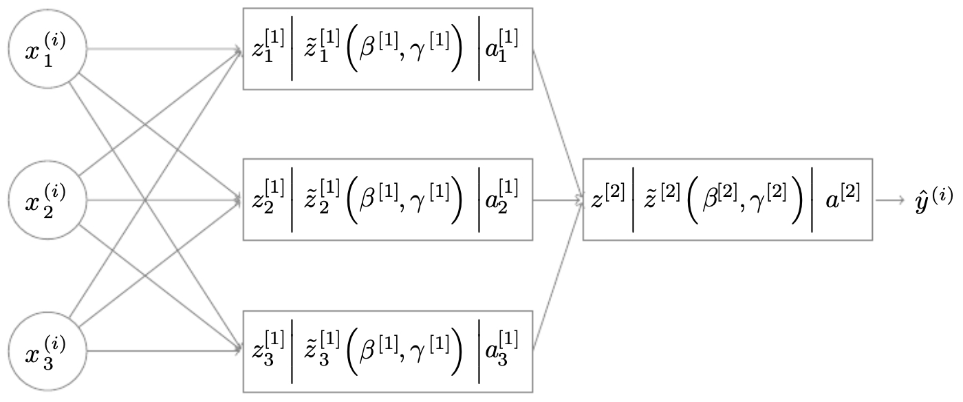
• The following figure illustrates how each node now computes three stages: (1) linear activation, (2) batch normalization, and (3) non-linear activation.

Fitting Batch Norm in a Neural Network

• For layer \(\ell\), the computation pipeline becomes:

• Notice that the bias term \(b^{[\ell]}\) is effectively redundant, since the shift is absorbed by \(\beta^{[\ell]}\).

• Thus, each BN layer requires learning parameters \(\{ W^{[\ell]}, \gamma^{[\ell]}, \beta^{[\ell]} \}\).

• During backpropagation, the updates are:

  \[W^{[\ell]} := W^{[\ell]} - \alpha \, dW^{[\ell]}, \quad \gamma^{[\ell]} := \gamma^{[\ell]} - \alpha \, d\gamma^{[\ell]}, \quad \beta^{[\ell]} := \beta^{[\ell]} - \alpha \, d\beta^{[\ell]}\]
  • where \(\alpha\) is the learning rate.

Batch Norm at Test Time

• At test time, inference is often done on single samples, so we cannot compute fresh \(\mu^{[\ell]}\) and \(\sigma^{2[\ell]}\).

• Instead, we use exponentially weighted averages (EMA) of the mean and variance, accumulated during training.

  \[z_{\text{norm}}^{[\ell](i)} = \frac{z^{[\ell](i)} - \mu^{[\ell]}_{\text{EMA}}}{\sqrt{\sigma^{2[\ell]}_{\text{EMA}} + \epsilon}}\]
  • where \(\mu^{[\ell]}_{\text{EMA}}\) and \(\sigma^{2[\ell]}_{\text{EMA}}\) are running estimates across mini-batches.

Multi-class Classification

• Up to this point, we have mainly considered binary classification problems, where the goal is to distinguish between two categories (e.g., cat vs. non-cat). However, many real-world applications require distinguishing among multiple classes simultaneously. Examples include handwritten digit recognition (0–9), object detection (cars, pedestrians, bicycles), and medical image diagnosis with multiple possible conditions.

• Neural networks extend naturally to multi-class classification by using the softmax regression output layer, which produces a probability distribution over all possible classes.

Softmax Regression

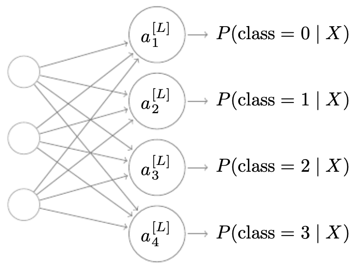
• Suppose we have \(C\) classes. The final layer of the neural network contains \(C\) neurons, each corresponding to the probability of one class.

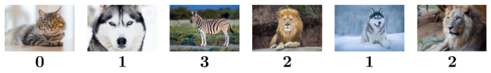
• The following figure illustrates a toy example: labels correspond to different animals, with classes 0 → cat, 1 → dog, 2 → lion, and 3 → zebra.

• For input \(X\), the last layer produces logits \(z^{[L]} \in \mathbb{R}^C\). We exponentiate each component:

• These are then normalized into probabilities via the softmax function:

• The vector \(a^{[L]} \in \mathbb{R}^C\) forms a probability distribution across the classes, with \(\sum_{i=1}^C a^{[L]}_i = 1\).

• The following figure visualizes this: each neuron in the final layer represents the probability of one class, so the model outputs not just a single guess but a full distribution across possible labels.

Worked Example

• Suppose the last layer produces the following logits:

• Exponentiating:

• Summing all exponentials:

• Final probabilities:

• Interpretation: the model predicts class 0 (cat) with the highest probability (84.2%).

Training a Softmax Classifier

• To train a softmax-based classifier, we use the cross-entropy loss. For a given true label \(y \in \{0, \dots, C-1\}\), represented as a one-hot vector, and prediction \(\hat{y} = a^{[L]}\):

• This penalizes the model heavily if it assigns low probability to the correct class.

• The full cost function over \(m\) training examples is:

• During backpropagation, the gradient of the loss with respect to the logits \(z^{[L]}\) is:

• This result is remarkably simple and mirrors the case of binary logistic regression, making implementation straightforward.

Practical Aspects of Training Softmax Classifiers

• While the softmax classifier is mathematically elegant and widely used, real-world applications introduce several practical considerations that can significantly impact training stability, performance, and generalization.

Numerical Stability

• The exponential function \(e^z\) grows rapidly with \(z\). For large logits (say, \(z > 100\)), computing \(e^z\) may result in overflow. To mitigate this, we adopt a log-sum-exp trick.

• For each input, we shift all logits by their maximum value before applying exponentiation:

  \[t_i = e^{z_i - \max_j z_j}\] \[a_i = \frac{t_i}{\sum_{j=1}^C t_j}\]

• Since subtracting a constant from all logits does not change the final softmax probabilities, this transformation improves numerical stability without altering results.

Class Imbalance

• In many datasets (e.g., fraud detection, medical imaging), some classes appear far more frequently than others. Standard cross-entropy loss can bias the model toward majority classes.

• Solutions include:

  • Class weighting: Assign higher loss weight to underrepresented classes:
  \[J = \frac{1}{m} \sum_{i=1}^m \sum_{j=1}^C w_j \, y_j^{(i)} \log \hat{y}_j^{(i)}\]
  • Resampling strategies: Oversample minority classes or undersample majority classes.
  • Synthetic data generation: Use methods like SMOTE (Synthetic Minority Over-sampling Technique) for tabular data or augmentation in vision tasks.

Calibration of Probabilities

• While softmax outputs are interpreted as probabilities, they are not always well-calibrated — i.e., a predicted confidence of 0.9 does not always mean the model is correct 90% of the time.

• Calibration techniques include:

  • Temperature scaling: Divide logits by a scalar \(T > 1\) before softmax to smooth predictions:
  \[a_i = \frac{e^{z_i / T}}{\sum_{j=1}^C e^{z_j / T}}\]
  • Platt scaling and isotonic regression, particularly for smaller models or highly imbalanced datasets.

• Calibration is crucial in safety-critical applications (e.g., healthcare, autonomous driving) where the confidence of predictions matters as much as correctness.

Large-Scale Classification

• In applications like face recognition or language modeling, the number of classes \(C\) can reach tens or hundreds of thousands. Computing a full softmax becomes computationally expensive.

• Solutions:

  • Hierarchical softmax: Arrange classes in a tree and compute probabilities along paths.
  • Negative sampling: Approximate softmax by considering only a subset of “negative” classes during training (popular in word2vec).
  • Sampled softmax / Noise-contrastive estimation (NCE): Estimate gradients with sampled classes instead of all classes.

Regularization for Multi-class Problems

• Softmax classifiers are prone to overfitting when classes are numerous and training data per class is small.

• Common remedies include:

  • Dropout applied before the softmax layer to encourage redundancy.
  • Label smoothing, where target one-hot vectors are softened:
  \[y_j^{\text{smoothed}} = (1 - \epsilon) \, y_j + \frac{\epsilon}{C}\]
  • This prevents the model from becoming overconfident and improves generalization.

Evaluation Metrics Beyond Accuracy

• While accuracy is intuitive, it may be misleading under class imbalance. Alternative metrics include:

  • Precision, Recall, and F1-score per class.
  • Confusion matrices to visualize misclassifications.
  • Top-k accuracy, which checks whether the true class is among the top \(k\) predicted classes (commonly used in ImageNet).

Citation

If you found our work useful, please cite it as:

@article{Chadha2020OptimizingStructuringNNs,
  title   = {Optimizing and Structuring Neural Networks},
  author  = {Chadha, Aman},
  journal = {Distilled Notes for Stanford CS230: Deep Learning},
  year    = {2020},
  note    = {\url{https://aman.ai}}
}