CS230 • Object Detection Algorithms

• Overview: image classification, classification with localization, and object detection
  • Task definitions and output spaces
  • Loss functions and learning objectives
  • Evaluation protocols
  • Model families and architectural choices
  • Post-processing and multi-instance reasoning
  • Practical considerations and when to use which
  • Mathematical summary of differences
  • Bridging strategies across the spectrum
• Object localization
  • Problem setup and coordinate system
  • Output vector and target semantics
  • Loss design
  • Activation functions and constraints
  • Data pipeline and labeling protocol
  • Architecture sketch
  • Example: self-driving perception mini-task
  • Evaluation metrics for localization
  • Relation to multi-object detection
• Landmark detection
  • Problem setup
    • Label parameterization
  • Applications and motivations
  • Model architectures
  • Loss functions
  • Evaluation metrics
• Object detection
  • The naïve sliding window approach
    • Limitations
  • Transition to convolutional implementations
• Bounding box predictions
  • Grid-based prediction
  • Constraints
  • YOLO: You Only Look Once
• Intersection over Union (IoU)
  • Mathematical definition
  • Evaluation thresholds
  • Why IoU matters
• Non-max suppression (NMS)
  • Core idea
  • Pseudocode
  • Example
  • Importance
• Anchor boxes
  • Defining anchor boxes
  • Assigning objects to anchors
  • Choosing anchor box sizes
  • Advantages
• YOLO: You Only Look Once
  • Core components
  • Unified output representation
  • Post-processing
  • Advantages
  • Limitations
• Advanced YOLO Variants
  • YOLOv2 (2017) – “YOLO9000”
  • YOLOv3 (2018)
  • YOLOv4 (2020)
  • YOLOv5 (2020, by Ultralytics)
  • YOLOv7 (2022)
  • YOLOv8 (2023, by Ultralytics)
  • Takeaways: YOLO evolution
• Citation

Overview: image classification, classification with localization, and object detection

• This section provides a unified, detailed overview of three core vision problem statements—image classification, image classification with localization, and object detection—clarifying their goals, label spaces, model outputs, loss designs, evaluation protocols, and typical architectures. We will also highlight how they relate to each other and when to choose which, grounding the discussion in canonical literature such as AlexNet (Krizhevsky et al., 2012), VGG (Simonyan & Zisserman, 2015), ResNet (He et al., 2016), R-CNN/variants (Girshick et al., 2014, Girshick, 2015, Ren et al., 2015), SSD (Liu et al., 2016), YOLO (Redmon et al., 2016), and RetinaNet with focal loss (Lin et al., 2017).

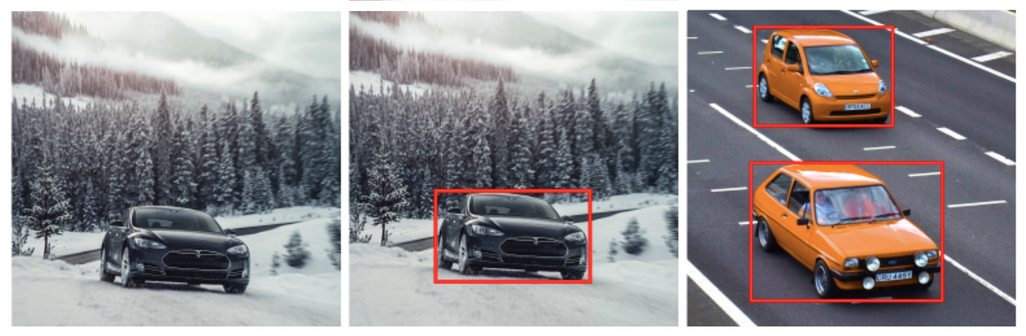
• The following figure contrasts the three tasks and serves as a mental model: (left) classification asks what, (middle) localization adds where for a single instance, and (right) detection scales to many instances of potentially many classes in one image. In other words, left shows a single global label for the dominant object (classification), middle shows a single tight box paired with a class (classification with localization), and right shows multiple class-labeled boxes for all visible instances (object detection).

Task definitions and output spaces

• Image classification:

  • Goal: assign one or more semantic labels to the entire image.
  • Typical output: for single-label, a probability vector \(\hat{\boldsymbol{p}}\in\mathbb{R}^K\) with \(\sum_k \hat{p}_k=1\); for multi-label, independent sigmoids \(\hat{p}_k\in[0,1]\).
  • Supervision: class ID(s) only.
  • Use cases: scene recognition, coarse screening, pre-filtering, weak supervision for downstream tasks.

• Classification with localization (single-object localization):

  • Goal: predict the presence and category of a single foreground object along with its bounding box.

  • Typical output for \(K\) classes:

    \[\hat{y}=\big[\hat{P}_c,\;\hat{b}_x,\;\hat{b}_y,\;\hat{b}_w,\;\hat{b}_h,\;\hat{c}_1,\ldots,\hat{c}_K\big],\]
    • where \(\hat{P}_c\in[0,1]\) denotes objectness, \((\hat{b}_x,\hat{b}_y)\in[0,1]^2\) are normalized center coordinates, and \(\hat{b}_w,\hat{b}_h\ge 0\) are normalized size parameters; \(\hat{c}_k\) are class scores.
  • Supervision: class ID plus one bounding box or a special background label.

• Object detection:

  • Goal: predict an unordered set of bounding boxes and labels for all object instances in the image.
  • Typical output: a variable-length set \(\{(\hat{B}_i,\hat{\boldsymbol{p}}_i,\hat{s}_i)\}_{i=1}^{N}\), where each \(\hat{B}_i=(\hat{b}_{x,i},\hat{b}_{y,i},\hat{b}_{w,i},\hat{b}_{h,i})\), \(\hat{\boldsymbol{p}}_i\) is a class distribution, and \(\hat{s}_i\) is a confidence score.
  • Supervision: one bounding box and class per annotated instance.

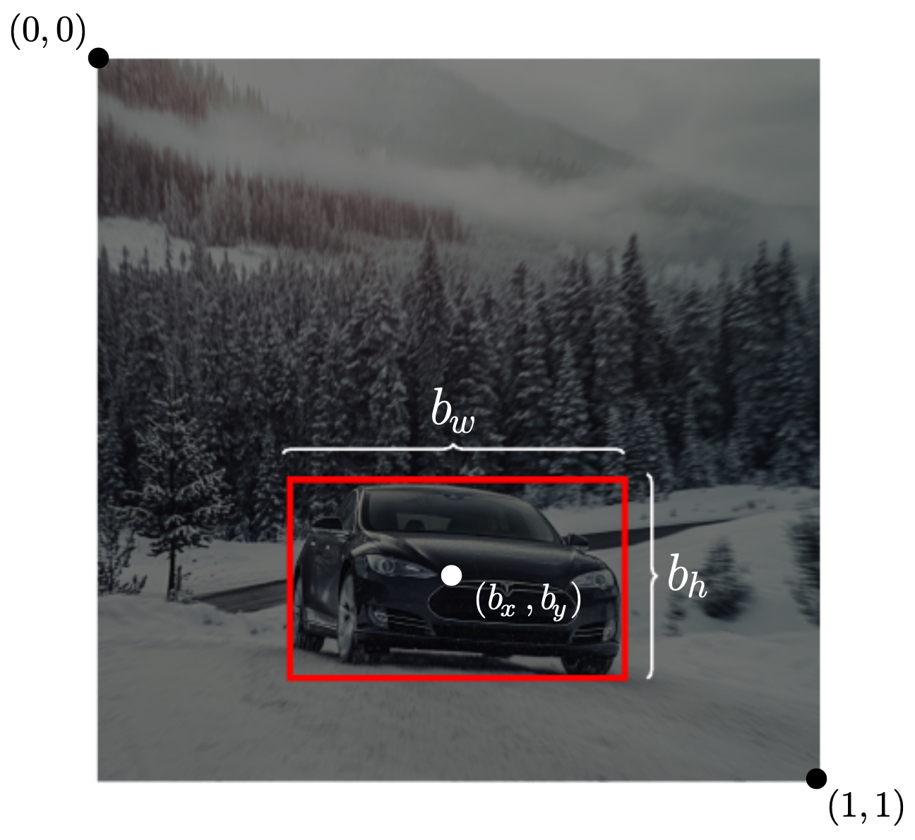
• The following figure introduces the normalized bounding-box parameterization used in localization and detection and clarifies the \((0,0)\) top-left, \((1,1)\) bottom-right convention. Specifically, the figure shows a unit-square canvas with a box defined by center \((b_x,b_y)\) and size \((b_w,b_h)\), emphasizing normalized coordinates for scale invariance and stable optimization across datasets.

Loss functions and learning objectives

• Classification:

  • Single-label: cross-entropy

    \[\mathcal{L}_{\text{cls}}=-\sum_{k=1}^K y_k\log \hat{p}_k.\]

  • Multi-label: binary cross-entropy per class

    \[\mathcal{L}_{\text{ml}}=\sum_{k=1}^K \big( -y_k\log \hat{p}_k - (1-y_k)\log(1-\hat{p}_k)\big).\]

• Localization:

  • Composite objective activating different terms depending on object presence:

    \[\mathcal{L}=\ell_{\text{obj}}(\hat{P}_c,P_c) + \mathbf{1}[P_c=1]\big(\ell_{\text{box}}(\hat{B},B)+\ell_{\text{cls}}(\hat{\boldsymbol{c}},\boldsymbol{c})\big).\]

  • Common \(\ell_{\text{box}}\): L1/L2 on coordinates; IoU-based losses such as GIoU/DIoU/CIoU improve geometric alignment and convergence.

• Detection:

  • Matching and assignment: algorithms align predictions to ground-truth instances using IoU thresholds or one-to-one matchers (e.g., Hungarian matching in DETR).
  • Losses: sum over matched pairs of classification and box losses; background/negative examples regularize confidence. Focal loss mitigates class imbalance in dense prediction (Lin et al., 2017).
  • A detailed discourse is offered in the section on Loss Design.

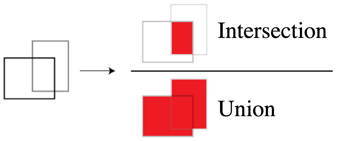
• The following figure visualizes Intersection-over-Union (IoU), the core overlap measure used for both training (matching) and evaluation (scoring) in localization and detection. It depicts two overlapping rectangles with shaded intersection and union regions, annotating the IoU ratio.

Evaluation protocols

• Classification:

  • Metrics: top-1/top-5 accuracy, per-class accuracy, ROC-AUC for multi-label.
  • Calibration: expected calibration error if scores will be thresholded downstream.

• Localization:

  • A prediction is correct if \(\hat{P}_c\) exceeds a confidence threshold and \(\mathrm{IoU}(\hat{B},B)\ge \tau\).
  • Report precision/recall/F1 at fixed \(\tau\) or average over \(\tau\in\{0.5,0.75\}\).

• Detection:

  • Mean Average Precision (mAP): area under the precision–recall curve averaged across classes and IoU thresholds; e.g., COCO mAP averages over \(\tau\in[0.5:0.95]\).
  • Auxiliary metrics: AR (average recall), per-size breakdowns (small/medium/large).

Model families and architectural choices

• Classification:

  • Backbones: convolutional networks (AlexNet, VGG, ResNet, EfficientNet) and modern vision transformers (ViT; Dosovitskiy et al., 2021).
  • Global pooling and linear classifier heads; strong data augmentation and regularization.

• Localization:

  • Shared backbone with three lightweight heads: objectness (sigmoid), box regression (linear to parameterized coordinates), and class scores (softmax/sigmoid).
  • Output dimensionality is fixed; assumes at most one foreground instance.

• Detection:

  • Two-stage: region proposals + refinement (Fast/Faster R-CNN; Ren et al., 2015).
  • One-stage dense predictors: SSD, YOLO, RetinaNet—predict over grids/anchors in a single pass; post-process with non-maximum suppression (NMS).
  • Transformer-based set prediction: DETR simplifies post-processing and uses bipartite matching (Carion et al., 2020).

Post-processing and multi-instance reasoning

• From localization to detection

  • Localization returns a single candidate; detection must reconcile many overlapping candidates for many classes.

• Non-maximum suppression (NMS)

  • Given class-specific candidate boxes with scores \(\hat{s}_i\), sort by score, select the highest, and suppress others with IoU above a threshold \(\theta\) relative to the selected box; repeat until exhaustion.

• Confidence calibration

  • Score thresholds influence precision/recall trade-offs; per-class thresholds or learned NMS/soft-NMS can improve tail behavior.

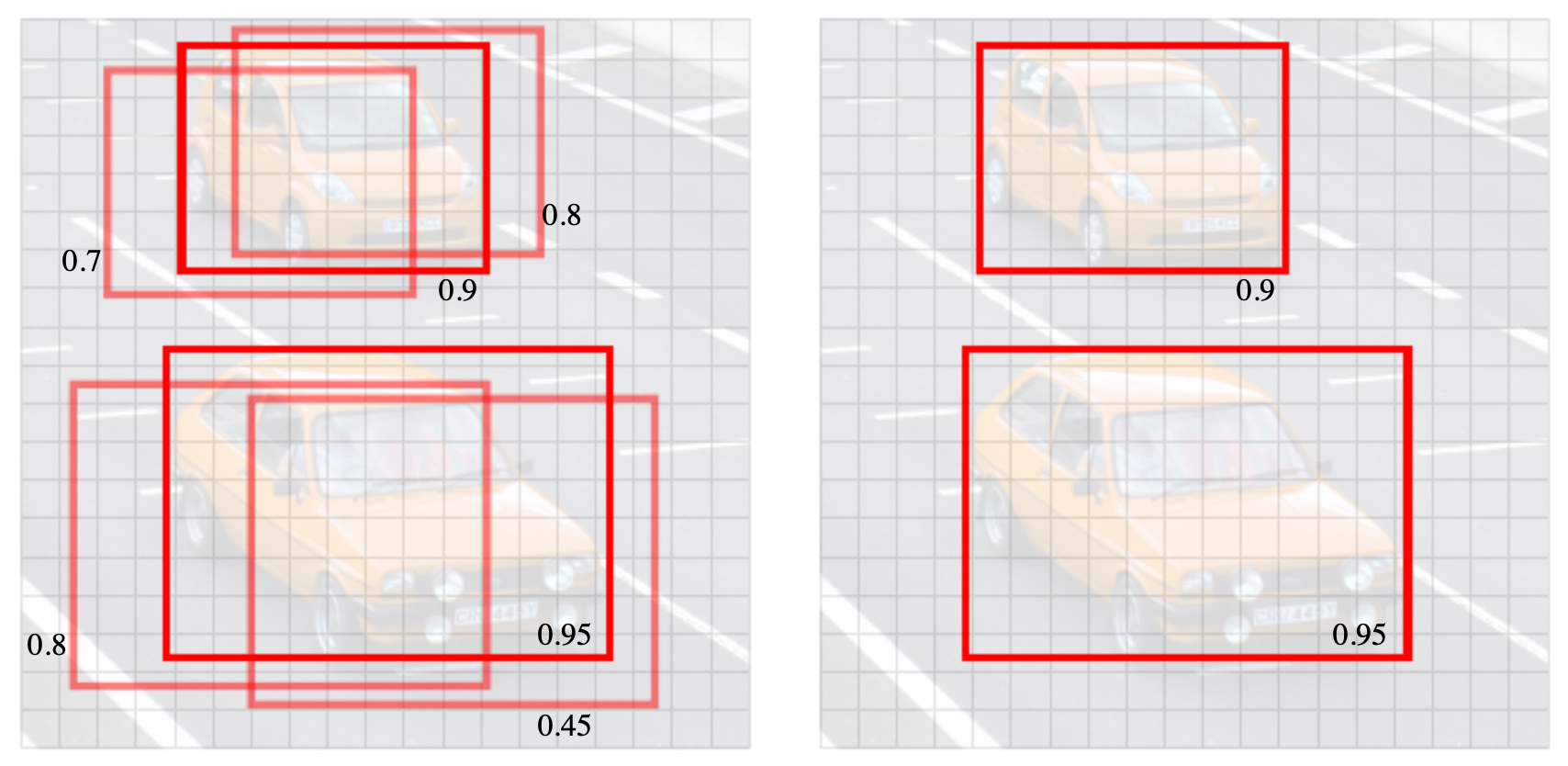
• The following figure presents pre- and post-NMS predictions on a dense set of candidate boxes: many high-overlap boxes collapse to a single representative, preserving distinct instances while pruning duplicates.

Practical considerations and when to use which

• Choose classification when: You only need global semantics or downstream routing, data lacks box annotations, or latency budget is tiny.

• Choose localization when: There is at most one salient foreground object per image, and you need a coarse location (e.g., crop for a subsequent module).

• Choose detection when: Multiple instances and classes must be enumerated, counted, or tracked; downstream tasks depend on per-instance reasoning.

• Labeling and data balance: Classification needs only class IDs; localization/detection require precise boxes, which increases annotation cost but yields richer supervision.

• Computation and latency: Classification is cheapest; localization adds minimal overhead; detection varies by family (one-stage often faster than two-stage).

• Robustness: Detection is more sensitive to occlusion and scale variance; multi-scale features (FPN) and anchor/anchor-free designs help.

Mathematical summary of differences

• Let \(\mathcal{I}\) denote the image, \(\mathcal{C}=\{1,\ldots,K\}\) the class set.

  • Classification learns \(f:\mathcal{I}\rightarrow \Delta^{K-1}\).
  • Localization learns \(g:\mathcal{I}\rightarrow [0,1]\times [0,1]^2\times \mathbb{R}_+^2 \times \mathbb{R}^K\).
  • Detection learns \(h:\mathcal{I}\rightarrow \mathcal{P}\big([0,1]^2\times \mathbb{R}_+^2\times \Delta^{K-1}\times [0,1]\big)\), where \(\mathcal{P}(\cdot)\) is the power set, reflecting a variable number of instances.

Bridging strategies across the spectrum

• Pretraining: classification pretraining (e.g., ImageNet) improves both localization and detection via transfer learning.
• Curriculum: start with localization to debug box parameterization and losses before scaling to full detection.

• Unification: modern detectors subsume localization as a special case (predict exactly one high-confidence box), and can be configured to operate in “single-instance mode” by adjusting thresholds and NMS.

• In typical object detection architectures, a shared feature extractor (“trunk”) is used along with multiple (say, three) task-specific heads for applications such as classification, single-object localization (objectness + box + class), and dense detection (grid or anchor-free) which produces per-cell box/class predictions combined with NMS or a set-based matcher.

• Up next, we will deepen the detection side by formalizing dense prediction over grids/anchors, IoU-based matching, non-maximum suppression details, anchor boxes, and the YOLO/SSD/RetinaNet families, connecting the concepts here to efficient, production-grade detectors.

Object localization

• Object localization extends image classification by predicting not only what object is present but also where it is located in the image. In this section, we will formalize the localization task, define targets and losses, discuss coordinate parameterizations and constraints, and walk through practical training details using a self-driving perception example.

• The following figure contrasts three increasingly expressive tasks—plain classification, classification with localization, and full detection—highlighting why localization is the natural next step beyond single-label classification.

Problem setup and coordinate system

• We start with single-object images. The model must output both a categorical label and a bounding box that tightly encloses the object instance.

• Coordinate normalization. We standardize all images to a fixed square canvas and use a unit square coordinate system, with the top-left pixel at \((0, 0)\) and the bottom-right pixel at \((1, 1)\). Bounding boxes are represented by the center \((b_x, b_y)\) and dimensions \((b_w, b_h)\), all in normalized units.

• The following figure illustrates the labeling convention and the normalized coordinate system we will use throughout.

Output vector and target semantics

• For \(K\) foreground classes (e.g., pedestrian, car, motorcycle), we represent the model output for a single image as

  \[\hat{y} \;=\; \Big[P_c,\;\hat{b}_x,\;\hat{b}_y,\;\hat{b}_w,\;\hat{b}_h,\;\hat{c}_1,\ldots,\hat{c}_K\Big]\]

  • where:

    • \(P_c \in [0,1]\) is the confidence that a foreground object is present.
    • \((\hat{b}_x,\hat{b}_y,\hat{b}_w,\hat{b}_h)\) are the predicted box parameters (center, width, height).
    • \(\hat{c}_k\) are class scores (e.g., logits or probabilities) over the \(K\) classes.

• Targets follow the same shape:

  \[y \;=\; \Big[P_c,\;b_x,\;b_y,\;b_w,\;b_h,\;c_1,\ldots,c_K\Big]\]
  • with one-hot class targets \(\{c_k\}\) if \(P_c=1\). If no object is present, we set \(P_c=0\) and treat the box and class targets as “don’t-care” (ignored by the box/class losses; see Loss design below).

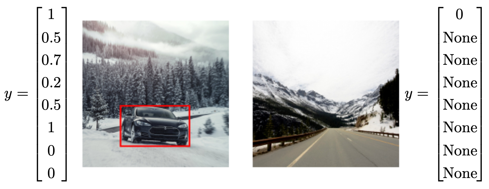
• Concrete examples (for \(K=3\): pedestrian, car, motorcycle):

  • Foreground example (car present) might look like

    \[y = \big[1,\;0.50,\;0.70,\;0.20,\;0.15,\;0,\;1,\;0\big]\]

  • Background example (no object) uses

    \[y = \big[0,\;\_\;,\;\_\;,\;\_\;,\;\_\;,\;\_\;,\;\_\;,\;\_\;\big]\]
    • where underscores denote fields that will be ignored by the non-applicable loss terms.

• The following figure shows representative labeled targets for a foreground car and for a background image, illustrating the presence/absence flag \(P_c\) and corresponding fields.

Loss design

• We use a conditional loss that activates the appropriate terms depending on whether an object is present:

  \[\mathcal{L}(\hat{y}, y) = \underbrace{\ell_{\text{obj}}(\hat{P}_c, P_c)}_{\text{objectness}} \;+\; \mathbf{1}[P_c = 1]\, \Big( \underbrace{\ell_{\text{box}}\big((\hat{b}_x,\hat{b}_y,\hat{b}_w,\hat{b}_h),\,(b_x,b_y,b_w,b_h)\big)}_{\text{localization}} + \underbrace{\ell_{\text{cls}}(\hat{\boldsymbol{c}}, \boldsymbol{c})}_{\text{classification}} \Big).\]

• A simple instantiation consistent with squared-error targets is

  \[\ell_{\text{obj}} = (\hat{P}_c - P_c)^2,\quad \ell_{\text{box}} = \sum_{u\in\{x,y,w,h\}} (\hat{b}_u - b_u)^2,\quad \ell_{\text{cls}} = \sum_{k=1}^{K} (\hat{c}_k - c_k)^2.\]

• In practice, cross-entropy for \(\ell_{\text{cls}}\) and IoU- or L1/L2-based box losses for \(\ell_{\text{box}}\) are often preferred for stability and calibration (see, e.g., Girshick et al., 2014, Ren et al., 2015), but the squared-error formulation is a useful starting point and aligns with our simple targets above.

Activation functions and constraints

• Because the parameters are constrained, the output heads should respect their ranges:

  • Objectness \(P_c \in [0,1]\). Use a sigmoid output and interpret as probability.
  • Centers \(b_x, b_y \in [0,1]\). Use a sigmoid or clamp after a linear head.
  • Sizes \(b_w, b_h \ge 0\). Common parameterizations include
  \[\hat{b}_w = \mathrm{softplus}(t_w),\quad \hat{b}_h = \mathrm{softplus}(t_h),\]
  • or exponentiating predicted log-scales. With normalized coordinates, bounding \(b_w,b_h \le 1\) may also be desirable to avoid degenerate proposals.

• These design choices improve training stability and ensure valid geometry.

Data pipeline and labeling protocol

• Single-object assumption. Each training image either contains exactly one object from the label set or is pure background.
• Consistent landmarking of corners (implicit here via box center/size), consistent class taxonomy, and quality control on annotations are critical.
• Balancing positives and negatives. Background images are essential to calibrate \(P_c\) and reduce false positives.
• Augmentations. Geometric transforms that preserve boxes (random flips, crops with box adjustment) and photometric changes (brightness, contrast) improve generalization. When cropping, re-normalize \((b_x,b_y,b_w,b_h)\) relative to the transformed canvas.

Architecture sketch

• A standard convolutional neural network (CNN) backbone feeds into three heads:

  • Objectness head predicting \(\hat{P}_c\).
  • Box regression head predicting \((\hat{b}_x,\hat{b}_y,\hat{b}_w,\hat{b}_h)\).
  • Classification head predicting \(\hat{\boldsymbol{c}}\in\mathbb{R}^K\).

• Training uses minibatches that mix positive and negative samples. Inference emits a single box and class for the image if \(\hat{P}_c\) exceeds a threshold.

Example: self-driving perception mini-task

• Suppose a self-driving car must decide whether the scene contains one of {pedestrian, car, motorcycle} or background. The network outputs:

  \[\hat{y}=\big[\hat{P}_c,\;\hat{b}_x,\;\hat{b}_y,\;\hat{b}_w,\;\hat{b}_h,\;\hat{c}_{\text{ped}},\;\hat{c}_{\text{car}},\;\hat{c}_{\text{moto}}\big].\]
  • If a pedestrian is present, we set \(P_c=1\), provide the pedestrian box, and use \(\boldsymbol{c} = (1,0,0)\).
  • If no object is present, we set \(P_c=0\) and drop the box/class terms from the loss.

Evaluation metrics for localization

• While full detection commonly uses mean Average Precision (mAP), single-object localization can be evaluated with Intersection-over-Union (IoU) and thresholded accuracy:

• IoU is defined as

  \[\mathrm{IoU}(B_{\text{pred}}, B_{\text{gt}}) \;=\; \frac{\mathrm{area}\big(B_{\text{pred}} \cap B_{\text{gt}}\big)}{\mathrm{area}\big(B_{\text{pred}} \cup B_{\text{gt}}\big)}.\]

• A prediction is considered correct if \(P_c\) exceeds a confidence threshold and \(\mathrm{IoU}\ge \tau\) (often \(\tau=0.5\), though this is a tunable convention).

• The following figure visualizes IoU as the ratio of the intersection area to the union area of predicted and ground-truth boxes, a geometry that tightly links localization accuracy to overlap quality.

Relation to multi-object detection

• Single-object localization is a conceptual stepping stone to full detection. The principal differences:

  • Cardinality: Detection allows multiple instances and classes per image.
  • Spatial assignment: Detection typically partitions images into grids or proposals (anchors) and predicts multiple boxes.
  • Post-processing: Detection introduces mechanisms like non-maximum suppression (NMS) to reconcile multiple overlapping predictions.
  • Efficiency: One-shot detectors such as YOLO (Redmon et al., 2016; later versions refine this line) unify localization and classification over many spatial locations in a single pass.

• We will build on these ideas in subsequent sections when we move from single-object localization to sliding windows, convolutional speedups, bounding-box prediction over grids, IoU-based matching, non-max suppression, anchor boxes, and the YOLO family.

Landmark detection

• Landmark detection expands the scope of computer vision from bounding entire objects to pinpointing precise, semantically meaningful keypoints within them. This task is central to applications like face recognition, expression analysis, pose estimation, and augmented reality. Its applications span from entertainment (face filters) to critical tasks in medicine and robotics. As we advance, these ideas will set the stage for handling multiple objects with varying numbers of landmarks and combining them with detection frameworks.

• The following figure shows three diverse applications of landmark detection—emotion classification from facial landmarks, tracking the motion of human bodies, and overlaying augmented filters in social media contexts.

Problem setup

• Unlike object localization, where we regress to one bounding box, landmark detection requires predicting multiple point coordinates associated with a known object (e.g., 68-point face landmarks, 21 hand landmarks, or 17 human pose keypoints).

Label parameterization

• For an image known to contain a target object (e.g., a human face), the ground truth label vector has the form

  \[y = \Big[\text{face?},\;\ell_{1x}, \ell_{1y},\;\ell_{2x}, \ell_{2y},\;\dots,\;\ell_{nx}, \ell_{ny}\Big],\]
  • where each pair \((\ell_{ix}, \ell_{iy})\) denotes the normalized coordinates of landmark \(i\). The binary indicator “face?” ensures the model is aware whether the target object is present.

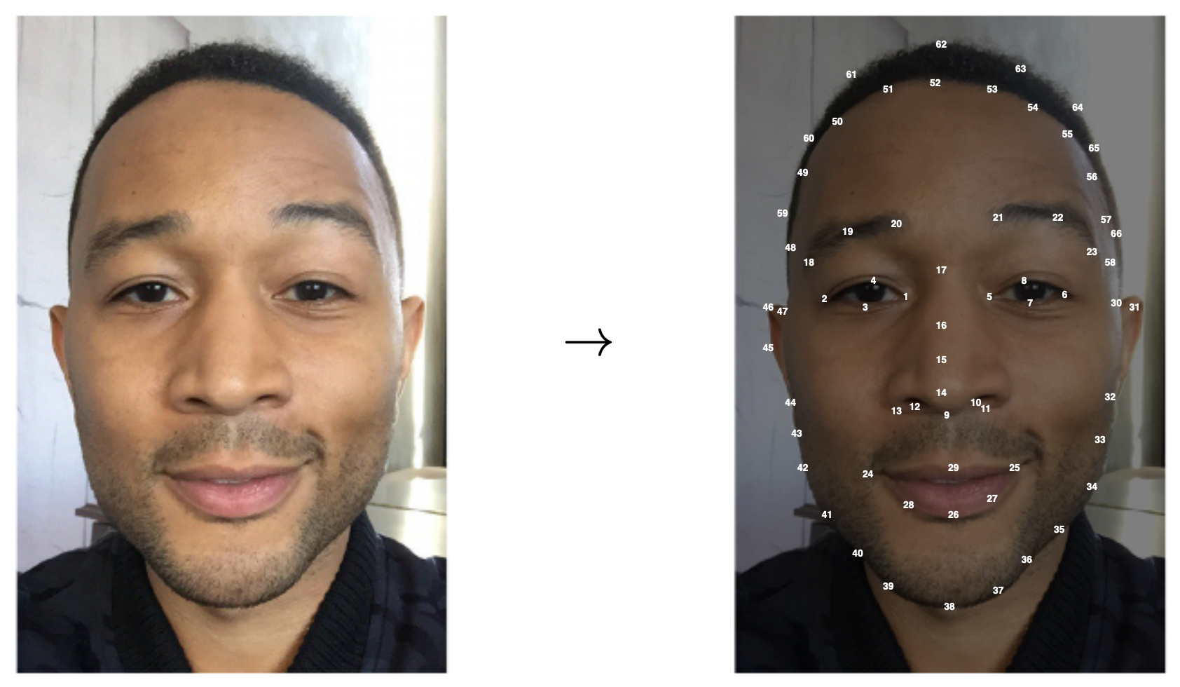
• Consistency is critical: the \(i^{th}\) landmark must always correspond to the same semantic part across all training images (e.g., “leftmost corner of the left eye” is landmark 1 in every face).

• The following figure illustrates a face with consistently indexed landmarks, ensuring reproducibility in training and inference.

Applications and motivations

• Facial expression recognition. Landmarks around eyes, eyebrows, and mouth provide geometric cues for classifying emotions such as happiness, anger, or surprise (Ekman & Friesen, 1978).
• Human pose estimation. Body keypoints (shoulders, elbows, knees, ankles) define articulated skeletons for sports analytics, animation, and motion capture (Cao et al., 2017).
• Augmented reality filters. Landmark positions enable realistic overlays such as glasses, masks, or animal features in AR platforms like Snapchat and Instagram.
• Medical imaging. Detecting anatomical landmarks (e.g., joints, vertebrae, organ boundaries) aids diagnosis and surgical planning.

Model architectures

• Architectures for landmark detection often use specialized heads on top of CNN backbones:

  • Direct regression. A fully connected head predicts the 2D coordinates of all landmarks simultaneously. Effective for small numbers of landmarks but sensitive to normalization.
  • Heatmap regression. Instead of predicting coordinates directly, the model outputs a spatial heatmap for each landmark, trained with pixelwise losses. Coordinates are extracted as the argmax or expectation over each heatmap. This approach is robust and aligns well with convolutional inductive biases (Newell et al., 2016).

Loss functions

• Depending on representation:

  • Coordinate regression loss. Standard L2 loss:

    \[\ell_{\text{coords}} = \frac{1}{n}\sum_{i=1}^{n} \big\| (\hat{\ell}_{ix}, \hat{\ell}_{iy}) - (\ell_{ix}, \ell_{iy}) \big\|_2^2.\]

  • Heatmap loss. Mean squared error (MSE) or cross-entropy between predicted and target heatmaps. Targets are typically Gaussian blobs centered at the ground-truth coordinates.

Evaluation metrics

• Accuracy of landmark detection is typically measured by:

  • Normalized Mean Error (NME). Average Euclidean distance between predicted and ground-truth landmarks, normalized by a reference distance (e.g., inter-ocular distance for faces).
  • Percentage of Correct Keypoints (PCK). Proportion of landmarks within a normalized distance threshold.
  • Area under the PCK curve (AUC). Summarizes detection accuracy across thresholds.

Object detection

• Object detection generalizes beyond localization by allowing multiple objects of potentially different classes to be identified within a single image. Unlike classification (one label per image) or localization (one object plus one bounding box), detection requires predicting both what and where for an arbitrary number of objects. This makes detection one of the most foundational tasks in computer vision.

• The following figure highlights the sliding windows detection approach, which uses cropped training examples to learn what objects look like in different contexts.

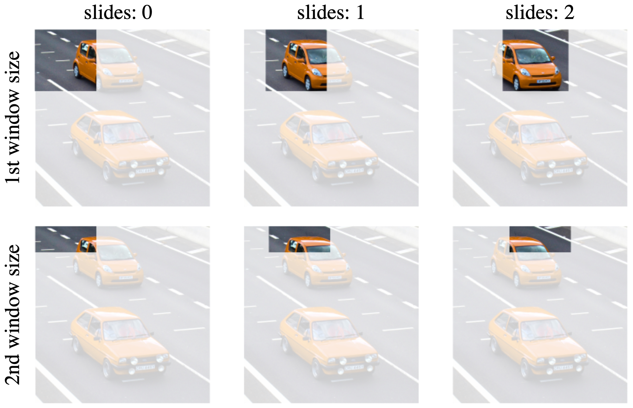
The naïve sliding window approach

• One of the earliest strategies for detection is the sliding windows algorithm. The idea is simple:

  1. Train a classifier on cropped images of the objects of interest.
  2. At test time, place a rectangular window at various positions and scales across the image.
  3. For each window, pass the pixels through the classifier.
  4. Label the window if the classifier is confident it contains an object.

• The following figure demonstrates this process, where the same classifier is applied to multiple window positions and sizes across the input image.

Limitations

• Computational cost. Each window requires a forward pass through the CNN, leading to huge redundancy across overlapping regions.
• Resolution vs. efficiency tradeoff. Reducing stride increases recall but exponentially increases runtime.
• Scale variation. Objects at different scales require repeated evaluations with resized windows.

• Inefficient feature sharing. Most windows overlap heavily, yet their convolutional features are recomputed redundantly.

• Despite these inefficiencies, sliding windows provided a stepping stone toward modern detectors by highlighting the need for shared computation.

Transition to convolutional implementations

• To mitigate redundancy, sliding windows can be reformulated as a convolutional operation:

  • Instead of cropping each window and re-feeding it to the CNN, treat the full image as input.
  • Convolutions naturally slide filters across positions, producing outputs corresponding to window locations.
  • By interpreting these outputs as classification scores, we achieve the same effect as explicit window sliding, but with massive efficiency gains.

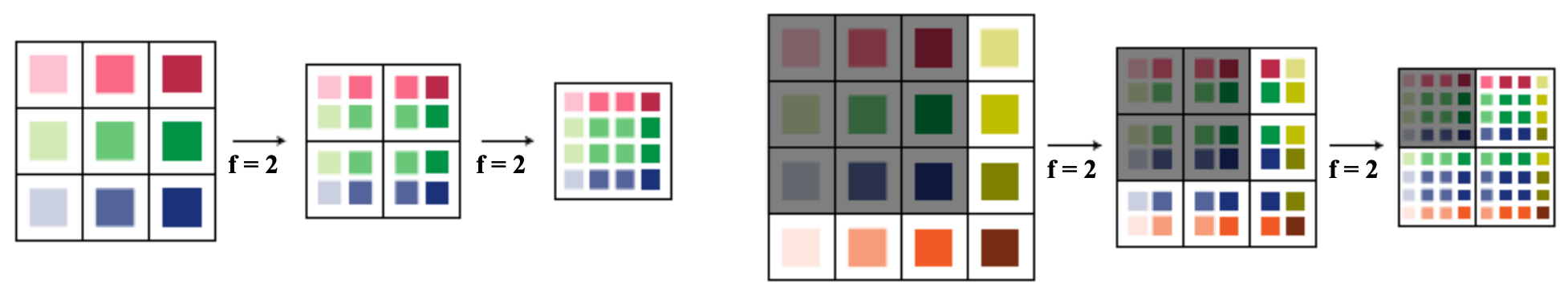
• The following figure compares the output of a model when applied to a \(3 \times 3\) input versus a \(4 \times 4\) input, showing how convolution enables overlapping receptive fields to be computed in parallel.

• This perspective set the stage for convolutional detection networks, where:

  • Convolutional layers generate dense feature maps shared across positions.
  • Each location in the feature map corresponds to a candidate window.
  • Later layers predict class probabilities and objectness for each window simultaneously.

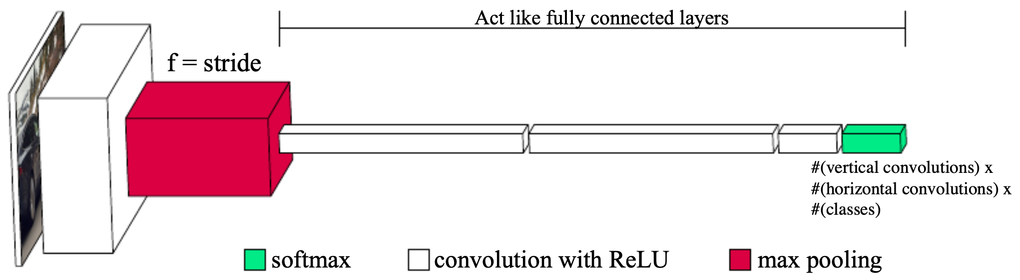
• The following figure depicts such an architecture: a CNN backbone produces feature maps, which are then pooled and fed into fully connected or \(1 \times 1\) convolutional layers to classify windows and distinguish foreground classes from background.

Bounding box predictions

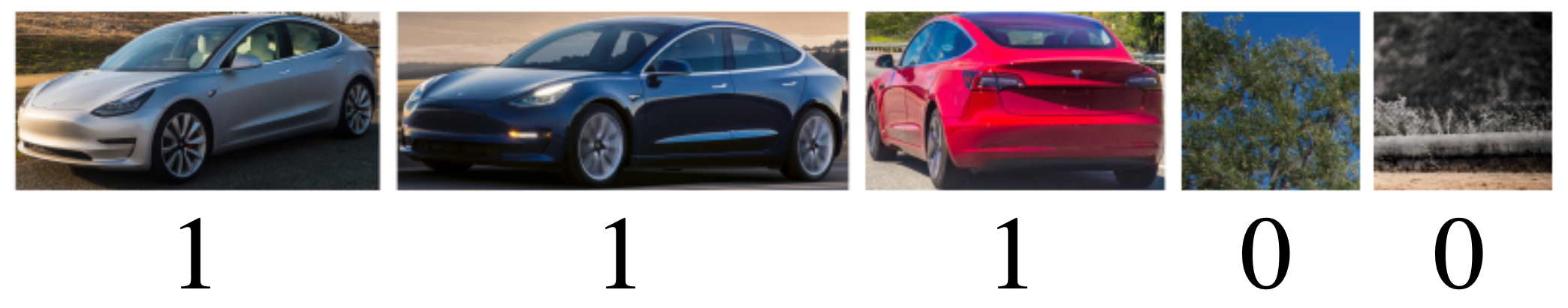
• Sliding windows (even in convolutional form) still rely on guess-and-check: scanning multiple scales and positions until the classifier fires. A more elegant approach is to have the network directly predict bounding boxes for objects in the image. This eliminates redundant computation and enables a single forward pass for detection.

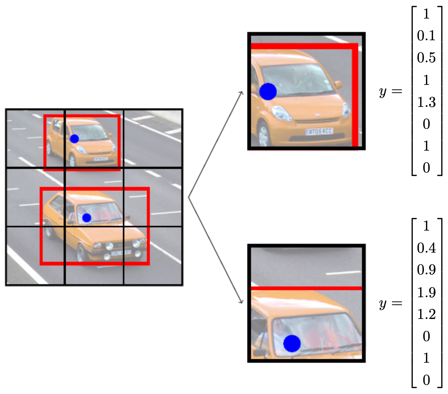
• The following figure shows an example of bounding box predictions for cars in an image, along with the corresponding normalized label vectors.

Grid-based prediction

• The key idea: partition the image into an \(S \times S\) grid. Each grid cell is responsible for predicting an object if the object’s center falls inside that cell.

• If an object’s center lies in a given cell, that cell outputs:

  • \(P_c = 1\) (object present)
  • Bounding box parameters \((b_x, b_y, b_w, b_h)\), relative to the grid cell
  • Class probabilities \(\{c_k\}\)

• If no object center is in the cell, then \(P_c = 0\).

• For example, with a \(3 \times 3\) grid and \(K=3\) classes (pedestrian, car, motorcycle), the total output tensor shape is:

  \[\text{Output shape} = S \times S \times (5 + K) = 3 \times 3 \times 8.\]
  • where 5 represents \((P_c, b_x, b_y, b_w, b_h)\).

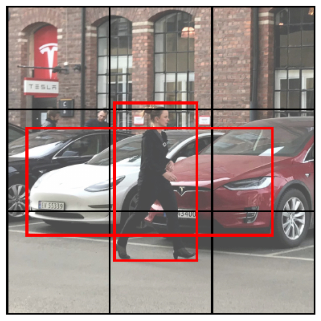
• The following figure shows how an image is divided into a \(3 \times 3\) grid, with each grid cell responsible for predicting an object if its center lies inside.

Constraints

• For normalized predictions:

  • \(0 \leq b_x, b_y \leq 1\): center coordinates relative to the grid cell.
  • \(b_w, b_h \geq 0\): width and height, usually normalized to the image size.

• The output tensor stacks predictions for all grid cells, enabling the network to emit multiple bounding boxes in parallel.

YOLO: You Only Look Once

• This approach is the foundation of the YOLO (You Only Look Once) family of detectors, first introduced by Redmon et al., 2016.

• A single CNN processes the entire image.
• The final layer outputs an \(S \times S \times (5 + K)\) tensor.
• Bounding box predictions, objectness, and class probabilities are all predicted simultaneously.
• Efficiency: detection is achieved in a single pass, making YOLO orders of magnitude faster than sliding window–based approaches.

Intersection over Union (IoU)

• Once bounding boxes are predicted, we need a quantitative way to evaluate how well they align with the ground truth. Intersection over Union (IoU) is the most widely used metric for this purpose. It captures the overlap between the predicted box and the ground-truth box, normalizing by their combined area.

• The following figure illustrates the concept of IoU: the intersection region divided by the union region of the predicted and ground-truth boxes.

Mathematical definition

• For a predicted box \(B_p\) and a ground-truth box \(B_{gt}\), the IoU is defined as:

• The numerator is the overlap region (intersection).

• The denominator is the combined coverage of both boxes (union).

• IoU values range from 0 (no overlap) to 1 (perfect alignment).

Evaluation thresholds

• In practice, we set a threshold \(\tau\) to determine whether a prediction counts as correct:

  • If \(\mathrm{IoU} \geq \tau\), the prediction is considered a true positive.
  • Otherwise, it is a false positive.

• A common choice is \(\tau = 0.5\), though stricter thresholds (e.g., 0.75) are sometimes used to demand tighter localization.

• Example:

  • IoU = 0.52 → Correct detection (for \(\tau = 0.5\))
  • IoU = 0.35 → Incorrect detection

Why IoU matters

• Fairness. IoU accounts for both underestimation (predicted box too small) and overestimation (predicted box too large).
• Ranking. IoU enables comparing multiple predictions for the same ground-truth object.

• Foundation for metrics. IoU underpins evaluation metrics like mean Average Precision (mAP), the de facto standard for object detection benchmarking.

• The following figure shows an example of multiple predictions with their IoU values compared to the ground-truth box. Notice that only predictions with IoU above the threshold are retained as correct detections.

Non-max suppression (NMS)

• Bounding box prediction with grids or anchors often produces multiple overlapping boxes that refer to the same object. If left unfiltered, these duplicate predictions can confuse evaluation and downstream tasks. Non-max suppression (NMS) is a post-processing algorithm designed to eliminate redundant detections, keeping only the most confident bounding box for each object.

• The following figure shows how multiple overlapping bounding boxes predicted for the same object (left) can be reduced to a single representative box using NMS (right). The image shows predicted bounding boxes using a \(19 \times 19\) grid along with the confidence a non-background class exists inside of that box.

Core idea

1. Begin with a list of predicted boxes, each with:

   • Confidence score \(P_c\)
   • Class label
   • Coordinates \((b_x, b_y, b_w, b_h)\)

2. Filter out low-confidence boxes (e.g., \(P_c \leq 0.6\)).

3. For each class:

   • Select the box with the highest \(P_c\).
   • Remove any other box of the same class with IoU \(\geq \tau\) (commonly \(\tau=0.5\)).
   • Repeat until no boxes remain.

Pseudocode

Input: list of boxes with (confidence, coordinates)
Output: finalBoxes

1. Remove all boxes with confidence ≤ threshold
2. Initialize finalBoxes = []
3. While boxes is not empty:
      a. maxBox = box with highest confidence
      b. Add maxBox to finalBoxes
      c. Remove maxBox from boxes
      d. For each box in boxes:
           - If IoU(box, maxBox) ≥ τ:
               remove box
4. Return finalBoxes

• This algorithm is simple yet effective, and has been used in nearly all modern detection pipelines.

Example

• Predicted boxes for a car:

  • Box A: confidence 0.95, IoU 0.8 with ground truth
  • Box B: confidence 0.90, IoU 0.75 with ground truth
  • Box C: confidence 0.45, IoU 0.82 with ground truth

• With \(\tau = 0.5\) and confidence threshold 0.6:

  • Box C is discarded (low confidence).
  • Box A is retained (highest confidence).
  • Box B is suppressed (IoU ≥ 0.5 with Box A).

• Final detection: Box A only.

Importance

• Cleaner results. Removes duplicate detections, ensuring each object appears once.
• Improved evaluation. Reduces false positives and inflates precision.
• Efficiency. NMS is lightweight and can be implemented efficiently for real-time systems.

Anchor boxes

• One limitation of the grid-based bounding box prediction scheme is that only one object can be assigned per grid cell. If two objects’ centers fall into the same cell, the model cannot represent both. Anchor boxes solve this problem by allowing each grid cell to predict multiple bounding boxes, each with a predefined shape (aspect ratio and scale).

Defining anchor boxes

• Anchor boxes are a fixed set of bounding box priors defined for each grid cell. Each anchor is designed to capture a specific aspect ratio or scale (e.g., tall and thin for pedestrians, wide and short for cars).

• Let each grid cell be associated with \(A\) anchor boxes.

• Each anchor outputs:

  • Objectness \(P_c\)
  • Box parameters \((b_x, b_y, b_w, b_h)\)
  • Class scores \(\{c_k\}\)
• Thus, for \(K\) classes, each cell predicts \((5 + K) \times A\) values.
• Example: with \(S = 3\), \(K = 3\), and \(A = 2\), the output tensor is of shape

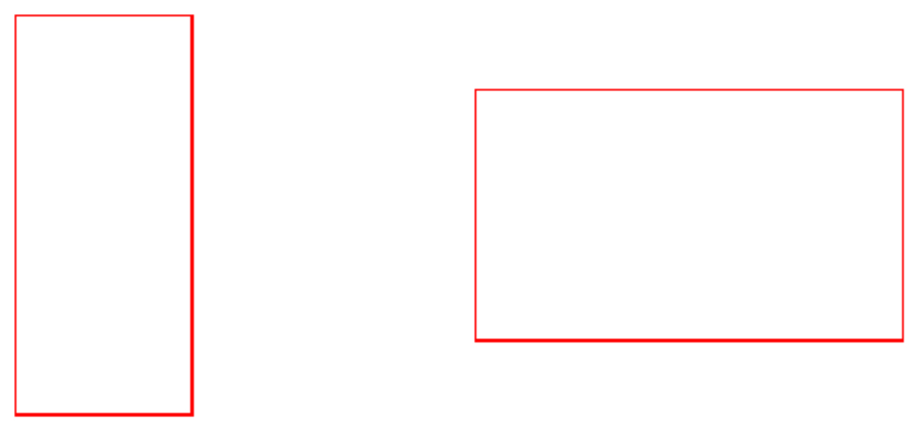
• The following figure shows how two anchor boxes of different aspect ratios are defined for each grid cell.

Assigning objects to anchors

• During training, each ground-truth box is assigned to the anchor box with the highest IoU overlap within the corresponding grid cell.

• Example:

  • A pedestrian (tall and narrow) matches best with anchor box 1.
  • A car (wide and short) matches best with anchor box 2.

• Both objects can now be represented in the same cell without conflict.

• The following figure illustrates this assignment: the midpoint for two objects–pedestrian and car–are located in the same grid cell. This results in the the pedestrian being matched to the tall anchor, the car to the wide anchor, both in the same grid cell.

Choosing anchor box sizes

• Anchor box dimensions are typically determined using clustering over the dataset:

  • Run k-means clustering on ground-truth box dimensions.
  • Choose the cluster centers as anchor box priors.
  • This ensures the anchors reflect common shapes and scales in the dataset (e.g., tall pedestrians, wide cars, medium-sized motorcycles).

Advantages

• Multi-object capability. Allows multiple detections per grid cell.
• Shape diversity. Different aspect ratios capture a wide range of object geometries.
• Compatibility. Anchor boxes are fundamental to many detectors (e.g., Faster R-CNN, SSD, YOLOv2).

YOLO: You Only Look Once

• The YOLO (You Only Look Once) algorithm, introduced by Redmon et al., 2016, revolutionized object detection by reframing it as a single regression problem. Unlike sliding windows or region proposal methods, YOLO directly maps an input image to a structured output of bounding boxes, objectness scores, and class probabilities in a single forward pass. This design achieves real-time detection without sacrificing too much accuracy.

Core components

• YOLO integrates the key concepts we’ve built up:

  1. Grid-based detection. The image is divided into an \(S \times S\) grid. Each grid cell predicts bounding boxes if an object’s center lies within that cell.

  2. Anchor boxes. Each grid cell has multiple anchor boxes (priors), enabling detection of multiple objects with different shapes or sizes in the same cell.

  3. Bounding box regression. Each anchor outputs box coordinates \((b_x, b_y, b_w, b_h)\), normalized relative to the cell and image dimensions.

  4. Objectness score. Each anchor predicts \(P_c\), the probability that an object is present in the box.

  5. Class prediction. Conditional class probabilities \(\{c_k\}\) are predicted for each anchor box, giving the final joint probability distribution.

Unified output representation

• For \(K\) classes and \(A\) anchors per cell, the output tensor is:

  \[\text{Output shape} = S \times S \times \big(A \times (5 + K)\big),\]

  • where each anchor contributes:

    • \(P_c\) (objectness)
    • \((b_x, b_y, b_w, b_h)\) (box coordinates)
    • \(\{c_1, \ldots, c_K\}\) (class scores)

• Example: for \(S=13\), \(A=5\), and \(K=20\) (Pascal VOC dataset), the output tensor is:

• The following figure illustrates how YOLO partitions the image, assigns objects to grid cells and anchors, and outputs predictions in a structured tensor.

Post-processing

• YOLO combines predictions with post-processing:

  • Non-max suppression (NMS): eliminates duplicate boxes for the same object.
  • Confidence thresholding: discards low-confidence detections.
  • IoU-based evaluation: determines correctness against ground truth.

Advantages

• Speed. Real-time inference (~45 FPS for YOLOv1 on a Titan X GPU in 2016).
• Simplicity. End-to-end differentiable, trained directly on detection targets.
• Generalization. Learns global representations, less reliant on region proposals.

Limitations

• Localization accuracy. Early YOLO versions struggled with small objects and crowded scenes.
• Fixed grid assignment. Objects with centers in the same cell compete for anchors.

• Recall. Less exhaustive than region proposal methods like Faster R-CNN.

• These limitations have been progressively addressed in later YOLO variants (YOLOv2–YOLOv8) through improved anchor design, multi-scale features, and better training objectives.

Advanced YOLO Variants

• The original YOLOv1 (2016) introduced a single-pass detection framework, but it struggled with small objects, crowded scenes, and localization precision. Over the years, the YOLO family evolved significantly, incorporating innovations from the broader detection community while retaining its speed advantage.

YOLOv2 (2017) – “YOLO9000”

• Key improvements (Redmon & Farhadi, 2017):

  • Anchor boxes introduced. Borrowed from Faster R-CNN, anchors allowed detection of multiple objects per grid cell.
  • Batch normalization. Applied to all layers, stabilizing training.
  • Higher-resolution classifier pretraining. Network trained at 448×448 before fine-tuning for detection.
  • Multi-scale training. Input resolution randomly changed during training, increasing robustness.
  • YOLO9000. Joint training on ImageNet classification and COCO detection enabled detection of over 9,000 classes.

YOLOv3 (2018)

• Improvements (Redmon & Farhadi, 2018):

  • Darknet-53 backbone. A deeper residual network improved feature extraction.
  • Multi-scale detection. Predictions made at three different feature-map resolutions (similar to Feature Pyramid Networks).
  • Logistic regression for objectness. Improved calibration of confidence scores.
  • Independent class predictions. Sigmoid activations replaced softmax, allowing multi-label detection.

YOLOv4 (2020)

• Improvements (Bochkovskiy et al., 2020):

  • CSPDarknet53 backbone. Based on Cross Stage Partial networks, balancing accuracy and efficiency.
  • Bag of freebies. Data augmentation techniques such as Mosaic augmentation and Self-Adversarial Training.
  • Bag of specials. Structural improvements like Spatial Pyramid Pooling (SPP) and Path Aggregation Network (PANet).
  • Real-time performance. Achieved high accuracy on COCO while maintaining speed.

YOLOv5 (2020, by Ultralytics)

• Though not from the original authors, YOLOv5 gained massive popularity due to:

  • PyTorch implementation. Easy adoption and training.
  • Modular design. Variants (s, m, l, x) balance speed and accuracy.
  • AutoAnchor optimization. Automated anchor selection based on dataset statistics.
  • Integrated ecosystem. Training scripts, augmentation, deployment-ready models.

YOLOv7 (2022)

• Introduced Extended Efficient Layer Aggregation Networks (E-ELAN) for deeper, more efficient architectures.
• Achieved state-of-the-art accuracy while remaining lightweight for real-time inference.
• Strong balance of speed vs. accuracy on GPUs.

YOLOv8 (2023, by Ultralytics)

• Latest widely adopted version:

  • Anchor-free detection. Moves away from anchor boxes, predicting box centers and dimensions directly.
  • Simplified design. Streamlined architecture for ease of use.
  • Better accuracy. Improved performance on COCO benchmark compared to YOLOv5/7.
  • Deployment-focused. Strong support for ONNX, TensorRT, and edge devices.

Takeaways: YOLO evolution

• YOLOv1: Single bounding box per grid cell.
• YOLOv2: Anchors, higher resolution, YOLO9000 joint training.
• YOLOv3: Residual backbone, multi-scale detection.
• YOLOv4: CSPDarknet, strong augmentations, state-of-the-art.
• YOLOv5: PyTorch ecosystem, practical deployment.
• YOLOv7: Efficient deeper networks, speed-accuracy leader.
• YOLOv8: Anchor-free, simplified design, best balance so far.

Citation

If you found our work useful, please cite it as:

@article{Chadha2020ObjectDetectionAlgorithms,
  title   = {Object Detection Algorithms},
  author  = {Chadha, Aman},
  journal = {Distilled Notes for Stanford CS230: Deep Learning},
  year    = {2020},
  note    = {\url{https://aman.ai}}
}