CS230 • Neural Networks
- Overview
- Deep learning intuition
- Day’n’night classification
- Face verification
- Face recognition
- Art generation (Neural Style Transfer)
- Trigger word detection
- App implementation
- Shallow neural networks
- Derivatives of activation functions
- Gradient descent for neural networks
- Random initialization
- Deep neural networks
- Forward and backward propagation in deep networks
- Parameters vs. Hyperparameters
- Connection to the Brain
- Citation
Overview
-
Neural networks form the foundation of modern deep learning. They are powerful function approximators capable of learning complex, nonlinear relationships from data. Unlike classical machine learning methods such as linear regression or logistic regression, which are limited by their simple functional forms, neural networks can represent highly flexible mappings between inputs and outputs by stacking multiple layers of computation. Concretely, a network implements a parametric function \(f_\Theta:\mathcal{X}\rightarrow\mathcal{Y}\), where \(\Theta\) collects all weights and biases. Training searches \(\Theta\) to minimize an empirical risk (e.g., cross-entropy) over a dataset \(\{(x^{(i)},y^{(i)})\}_{i=1}^m\). Depth and width allow \(f_\Theta\) to approximate intricate decision boundaries that simple linear models cannot represent.
-
At the core, a neural network consists of:
-
Architecture: the design of the model, including the number of layers, number of neurons per layer, and choice of activation functions. Architecture also specifies connection patterns (dense vs. convolutional), normalization placement, and down/up-sampling operations. Decisions here determine the model’s inductive bias—for example, convolutions encode locality and translation equivariance, while recurrent connections encode temporal structure.
-
Parameters: the weights and biases that are learned from data during training. For a fully connected layer transforming \(a^{[\ell-1]}\in\mathbb{R}^{n^{[\ell-1]}}\) to \(a^{[\ell]}\in\mathbb{R}^{n^{[\ell]}}\), parameters are \(W^{[\ell]}\in\mathbb{R}^{n^{[\ell]}\times n^{[\ell-1]}}\) and \(b^{[\ell]}\in\mathbb{R}^{n^{[\ell]}}\). In convolutional layers, parameters are compact kernels shared across spatial locations, dramatically reducing parameter count relative to dense layers on images.
-
Hyperparameters: design choices such as learning rate, optimization algorithm, and number of iterations that influence how parameters are updated. Additional hyperparameters include batch size, regularization strengths (e.g., \(\lambda\) for \(\ell_2\), dropout rate \(p\)), learning-rate schedules, weight decay, and data-augmentation policies. These control optimization dynamics and generalization.
-
-
Training a neural network involves two key processes:
-
Forward propagation: inputs are passed through the layers of the network to produce an output (e.g., a prediction). Each layer applies an affine transformation followed by a nonlinearity \(g\), e.g., \(z^{[\ell]}=W^{[\ell]}a^{[\ell-1]}+b^{[\ell]}\), \(a^{[\ell]}=g(z^{[\ell]})\). With mini-batches, these computations are vectorized for efficiency.
-
Backward propagation: gradients of the loss function with respect to the parameters are computed and used to update the weights and biases. Using the chain rule, we propagate \(\frac{\partial \mathcal{L}}{\partial a^{[\ell]}}\) backwards to obtain \(\frac{\partial \mathcal{L}}{\partial W^{[\ell]}}\) and \(\frac{\partial \mathcal{L}}{\partial b^{[\ell]}}\). Optimizers such as SGD with momentum, RMSProp, or Adam transform raw gradients into parameter updates, often coupled with learning-rate schedules (cosine decay, step decay, or warm restarts).
-
-
This iterative process allows the network to minimize its loss function and improve predictive accuracy. Practically, training proceeds for \(E\) epochs over shuffled data, with validation used to monitor generalization and trigger early stopping or checkpoint selection. Regularization—weight decay, dropout, data augmentation, mixup/cutmix—mitigates overfitting by smoothing the learned function or enriching the effective training distribution.
-
The intuition behind deep learning can be built up gradually:
- Starting from binary classification problems such as cat vs. not-cat, where the final activation is sigmoid and the loss is logistic cross-entropy,
- Extending to multi-class classification with one-hot or multi-hot labels, where the final activation is softmax (mutually exclusive) or independent sigmoids (non-exclusive),
- Exploring how deeper layers capture more complex features through encodings (latent representations that cluster semantically similar inputs),
- And applying these concepts to practical tasks such as day–night classification, face verification, style transfer, and trigger-word detection, each of which introduces domain-specific input pipelines (images, audio), task-tailored architectures (CNNs, RNNs/Transformers), and appropriate objective functions.
-
In summary, a modern pipeline comprises data preprocessing, architectural design aligned with the data modality, principled initialization (e.g., He/Xavier), normalization (BatchNorm/LayerNorm) to stabilize activations, nonlinearity selection (ReLU-family, GELU), an optimizer with a tuned learning-rate schedule, and vigilant validation/regularization strategies. These elements collectively turn the generic template \(\text{Input} + \text{Architecture} + \text{Parameters} \rightarrow \text{Output}\) into state-of-the-art performance across diverse applications.
Deep learning intuition
-
A model for deep learning is defined by two key components: architecture and parameters. The architecture specifies the computation graph (how information flows), while the parameters instantiate a particular function within that graph. Formally, given input \(x \in \mathbb{R}^{n_x}\), an \(L\)-layer network computes:
\[a^{[0]} = x,\qquad z^{[\ell]} = W^{[\ell]} a^{[\ell-1]} + b^{[\ell]},\qquad a^{[\ell]} = g^{[\ell]}(z^{[\ell]}),\quad \ell=1,\dots,L,\]- where activations \(g^{[\ell]}\) (e.g., ReLU, sigmoid, softmax) introduce nonlinearity so the composite map \(x \mapsto a^{[L]}\) can model complex decision boundaries. The learnable parameters are \(\Theta = \{W^{[\ell]}, b^{[\ell]}\}_{\ell=1}^L\).
-
The architecture is the algorithmic design we choose, such as logistic regression, linear regression, shallow neural networks, or deeper networks with many hidden layers. In practice, the architecture also specifies normalization (BatchNorm/LayerNorm), residual or skip connections, and the arrangement of specialized layers (e.g., convolutional vs. recurrent vs. attention blocks), all of which encode inductive biases appropriate for the data modality.
-
The parameters are the weights and biases that the model learns in order to transform an input into the correct output. During training, an optimizer (SGD, Adam, RMSProp) updates \(\Theta\) to minimize an empirical risk, typically
\[\min_{\Theta}\; \frac{1}{m}\sum_{i=1}^m \mathcal{L}\big(f_\Theta(x^{(i)}),\, y^{(i)}\big) \;+\; \lambda\,\Omega(\Theta),\]- where \(\mathcal{L}\) is a task-appropriate loss (e.g., cross-entropy), and \(\Omega\) is a regularizer (e.g., \(\ell_2\) weight decay) that helps control generalization.
-
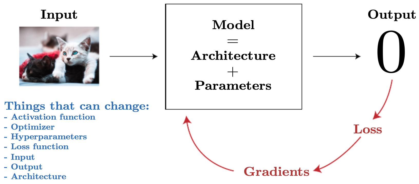
Mathematically: Input + Architecture + Parameters = Output. While this slogan is simple, each term hides crucial design choices:
- Activation function \(g\) influences gradient flow and representational capacity (e.g., ReLU vs. GELU).
- Optimizer and learning-rate schedule determine convergence speed and stability.
- Hyperparameters (batch size, weight decay, dropout rate) mediate the bias–variance trade-off.
- Input/output formats (e.g., logits vs. probabilities) affect both numerical stability and the choice of loss.
-
The following figure situates the model and its tunable components (architecture blocks, parameters, losses, activations, optimization settings) within the broader machine learning pipeline, emphasizing how data preprocessing and evaluation loop back to inform design revisions. Use it as a mental map: when performance stalls, check each box—data, architecture, objective, and optimization—systematically.
Multi-class classifiers and encoding schemes
-
Suppose we want to expand beyond binary classification. For example, instead of predicting whether an image is “cat” or “not cat”, we want to classify among three categories: cat, dog, and giraffe. Let \(n_x\) be the input dimensionality.
-
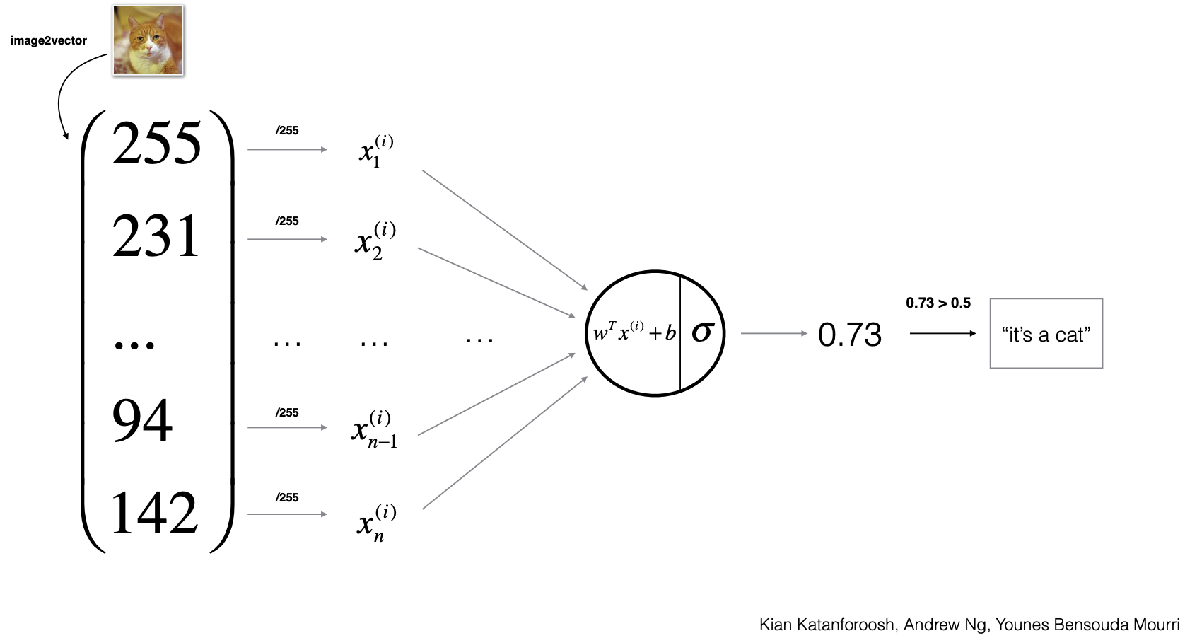
In binary classification, the weight vector is
\[w = \begin{bmatrix} w_1\\ w_2\\ \vdots\\ w_{n_x} \end{bmatrix},\]- with a scalar bias \(b\). The model computes a logit \(z = w^\top x + b\) and a probability \(\hat{y}=\sigma(z)=\frac{1}{1+e^{-z}}\).
-
The following figure demonstrates an example binary classification use-case, highlighting the linear score \(z\), the sigmoid squashing to \([0,1]\), and the decision boundary. Notice how feature scaling and separability influence the margin and thus confidence.
-
For multi-class classification with classes \(\{1,2,3\}\) (cat, dog, giraffe), we extend the weights into a matrix \(W \in \mathbb{R}^{n_x \times 3}\) and bias \(b \in \mathbb{R}^{3}\). The logits are \(z = W^\top x + b \in \mathbb{R}^3\). A natural output map is the softmax:
\[\hat{y}_k = \frac{e^{z_k}}{\sum_{j=1}^3 e^{z_j}},\quad k=1,2,3,\]- yielding a categorical distribution that sums to 1. The cross-entropy loss for one-hot label \(y\) is \(\mathcal{L} = -\sum_{k=1}^3 y_k \log \hat{y}_k\).
-
For the labels \(y\), we can choose different encodings:
- Integer encoding: \(y \in \{0,1,2\}\) (index form); used mostly for storage, not for loss computation directly.
- One-hot encoding: a length-3 vector with a single 1 at the correct class (aligned with softmax).
-
Multi-hot encoding: allows multiple simultaneous classes (e.g., cat and dog both present). Here, replace softmax with independent sigmoids per class and use a binary cross-entropy per output:
\[\mathcal{L} = -\sum_{k=1}^K \big[y_k \log \hat{y}_k + (1-y_k)\log(1-\hat{y}_k)\big].\]
- The choice between softmax and sigmoids exactly mirrors whether classes are mutually exclusive or not.
Activation functions in multi-class settings
- Sigmoid: Each neuron’s output is independent; multiple classes may be predicted simultaneously if their probabilities exceed a threshold. Best for multi-label settings.
- Softmax: Outputs are dependent and sum to 1, producing a categorical distribution—ideal when exactly one class is present. For numerical stability, compute softmax via the log-sum-exp trick, subtracting \(\max_k z_k\) before exponentiation.
Encodings in deep networks
-
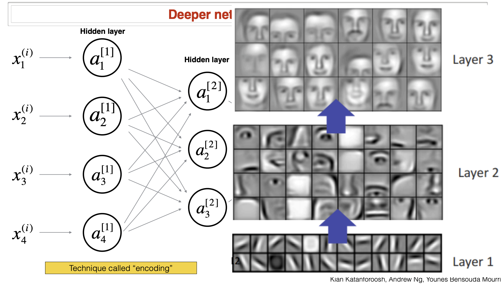
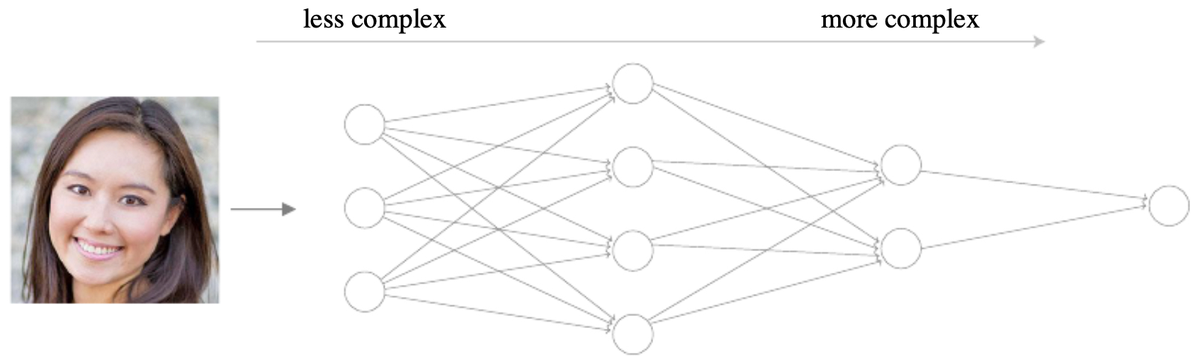
In deeper networks, earlier layers detect simple local features (edges, color blobs), mid-level layers compose parts (eyes, wheels), and deeper layers encode abstract concepts (faces, cars). These internal vectors are encodings—latent representations \(h(x)\) that cluster semantically similar inputs and linearize task-relevant variation.
-
The following figure illustrates how encodings emerge at different layers of the network, becoming progressively more abstract. Read left-to-right as a transformation pipeline: raw pixels \(\rightarrow\) low-level filters \(\rightarrow\) mid-level parts \(\rightarrow\) semantic embeddings that are linearly separable for the end task.
Day’n’night classification
- As a first concrete application, consider building an image classifier that predicts whether a photo taken outdoors was captured during the day (0) or during the night (1). This problem is deliberately simple, but it demonstrates the full machine learning pipeline: dataset preparation, input representation, model architecture, loss choice, and evaluation. By grounding theory in a practical case, we see how each design decision affects performance.
Data
- A robust model requires a sufficiently large and diverse dataset. From the cat vs. non-cat example earlier, we estimated that around 10,000 labeled images were needed for good accuracy. Since day–night classification is of similar difficulty, we likewise begin with approximately 10,000 labeled samples.
- Images should cover a variety of environments (urban, rural, coastal, desert) and lighting conditions (sunrise, sunset, cloudy, clear). Diversity reduces the chance of overfitting to spurious correlations like “dark backgrounds always mean night.”
- The dataset is split into training (80%) and testing (20%) subsets. To ensure both splits reflect the same class distribution, we use a stratified split, where day and night proportions are preserved across train and test.
Input
- The key design question is: what resolution is minimally sufficient to distinguish day from night? Higher resolution means more computation, but lower resolution risks losing discriminative cues (e.g., sky brightness, artificial lighting). Empirically, humans can distinguish day vs. night at surprisingly low resolutions. By experimentation, 64 × 64 × 3 RGB pixels balances efficiency with informativeness.
- The following figure shows an example input image for the classification task, emphasizing visual cues (blue sky, sunlight, shadows) that the model must detect.

Output
-
The output is binary:
- 0 → day
- 1 → night
-
Because the target values lie in \([0,1]\), the appropriate final activation is the sigmoid function:
\[\sigma(z) = \frac{1}{1 + e^{-z}}.\] -
The network produces a probability \(\hat{y} \in (0,1)\). At inference, we threshold at 0.5: if \(\hat{y} \geq 0.5\), predict night; otherwise, predict day.
Architecture
- Given the relatively simple task, a shallow neural network is sufficient. One hidden layer of moderate width (e.g., 20–50 neurons) already achieves high accuracy. However, as seen in similar tasks (e.g., cat classification), slightly deeper networks (3–4 layers) often improve performance by extracting richer features.
-
A simple baseline architecture might be:
- Input: \(64 \times 64 \times 3 = 12{,}288\) features (flattened).
- Hidden layer: 32 ReLU units.
- Output: 1 sigmoid unit.
- Despite its small size, this model captures enough information to separate day from night, since the global distribution of pixel intensities is highly discriminative.
Loss function
-
Because the final layer uses a sigmoid activation, the natural choice is binary cross-entropy (logistic) loss:
\[L(\hat{y}, y) = - \Big[ y \log(\hat{y}) + (1-y) \log(1-\hat{y}) \Big],\]where \(y\) is the true label (0 or 1) and \(\hat{y}\) is the predicted probability.
-
This loss penalizes confident mistakes heavily (e.g., predicting 0.99 for day when the true label is night), which encourages the network to refine its decision boundary.
Training loop
- Forward pass: compute predictions for a batch of inputs.
- Loss computation: evaluate cross-entropy.
- Backward pass: compute gradients via backpropagation.
- Parameter update: adjust weights with an optimizer (SGD or Adam).
Intuition
-
Day vs. night can often be inferred from global brightness, but training a neural network allows for robustness to edge cases:
- Brightly lit cityscapes at night.
- Overcast daytime scenes with low brightness.
- Photos with artificial lighting.
-
The network learns to weigh cues like sky hue, artificial light patterns, and shadow orientation. Even in ambiguous cases, it produces calibrated probabilities (e.g., \(\hat{y}=0.6\) night for a dimly lit dusk photo).
Face verification
-
Building on the day–night classifier, we now tackle a more complex and practically relevant task: face verification. Whereas day–night classification required only distinguishing between two global categories, face verification demands comparing two different images of faces and determining whether they belong to the same person.
-
A motivating scenario: A university wants to install automated systems at dining halls, gyms, and libraries. A student swipes their ID card, and a camera captures their face in real time. The system must verify whether the captured face matches the stored ID photo before granting access.
Data
-
The database contains one official ID photo per student, serving as the reference image.
-
During verification, a new photo (e.g., from a security camera) is captured.
-
The challenge is that these two photos may differ due to:
- variations in facial pose (frontal, side-tilted),
- differences in illumination (bright sunlight, dim hallways),
- changes in appearance (glasses, beard, hairstyle),
- aging or outdated ID photos.
-
This makes simple pixel-level comparison infeasible.
-
The following figure shows an example of a stored ID photo of a student:

- The following figure shows a current camera capture of the same student attempting access:

Input
- To capture sufficient facial detail, we require higher resolution than in day–night classification. A typical choice is 412 × 412 × 3 pixels. This preserves fine-grained facial features needed for reliable verification.
Output
-
The task is binary classification:
- 1 → ID verified (same person).
- 0 → ID not verified (different person).
-
A sigmoid activation in the final layer is appropriate, mapping the output to a probability in \([0,1]\).
Why pixel-by-pixel comparison fails
-
A naïve approach would be:
- Flatten both images into vectors.
- Compute the Euclidean distance between them.
- If the distance is below a threshold, predict “same person.”
-
This fails because:
- Illumination changes can drastically shift pixel values.
- Small pose differences (e.g., turning the head) cause large pixel misalignments.
- Accessories (glasses, hats) or facial hair drastically alter pixel-level similarity.
-
Thus, we need learned feature representations that are robust to these variations.
Encodings with deep networks
-
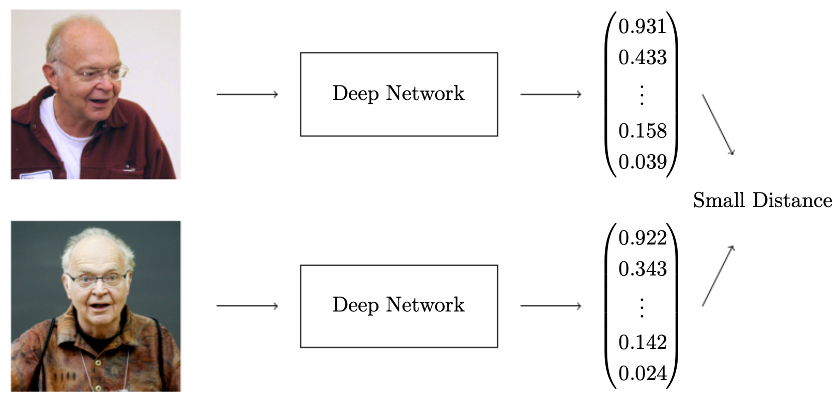
Modern face verification systems rely on deep convolutional neural networks (CNNs) to transform raw face images into encodings: low-dimensional vectors that capture essential facial structure while discarding irrelevant details (like lighting).
-
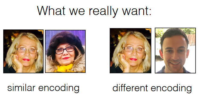
Intuition:
- Encodings of the same person should lie close together in the embedding space.
- Encodings of different people should lie far apart.
-
The following figure illustrates how a deep network projects face images into an embedding space where identity clusters emerge:
Triplet loss training
-
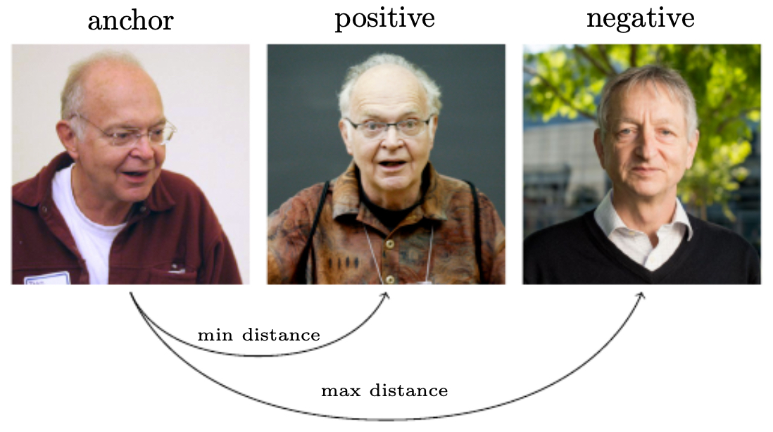
To train the network, we use triplets of images:
- Anchor (A): one image of a person.
- Positive (P): another image of the same person.
- Negative (N): an image of a different person.
-
The objective is to minimize the distance between A and P while maximizing the distance between A and N.
-
The following figure shows the triplet training setup:
Loss function
- The triplet loss is defined as:
-
where:
- \(Enc(X)\) is the encoding of image \(X\),
- \(\alpha\) is a margin hyperparameter (e.g., 0.2) ensuring separation between positive and negative pairs.
-
If the negative is already far apart from the anchor, the loss is zero; otherwise, the model is penalized until the margin is satisfied.
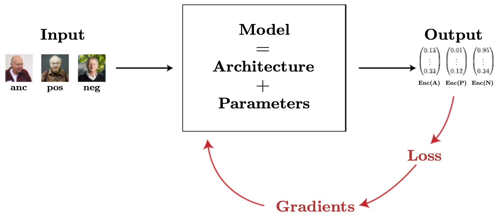
Final architecture
-
The final system consists of:
- A deep CNN that maps each image (anchor, positive, negative) into an encoding vector.
- A distance function (e.g., Euclidean distance) applied between encodings.
- The triplet loss ensuring proper clustering of identities.
-
At deployment time, the system only needs to compare the encoding of the query image with that of the stored ID photo.
-
The following figure shows the full architecture of the face verification pipeline:
Face recognition
-
In the previous section, we studied face verification, where the goal was to confirm whether two images belong to the same person (e.g., comparing a live capture to an ID photo).
-
In face recognition, the problem becomes harder: the model must identify the person directly from the image, without being told their claimed identity. This transforms the task into multi-class classification or, in large databases, a nearest-neighbor search problem in an embedding space.
-
Real-world applications include:
- unlocking smartphones,
- tagging people in social media photos,
- surveillance and access control,
- automatic photo album organization.
Data
-
Face recognition requires multiple images per person in the training set. Unlike verification (which only needs one reference photo per identity), recognition must learn to generalize across:
- pose changes,
- different lighting conditions,
- appearance variations (haircut, glasses, beard),
- aging effects.
-
This is why large public datasets such as LFW (Labeled Faces in the Wild), MS-Celeb-1M, and VGGFace2 are often used for training.
-
The following figure illustrates the recognition task: a query image must be matched to the correct identity in the database of stored student faces.
Input and encodings
- As in verification, we use high-resolution input images, e.g., 412 × 412 × 3, to preserve sufficient detail.
- A deep CNN converts each face into a fixed-dimensional encoding vector.
-
The recognition system must ensure:
- encodings of the same person cluster closely,
- encodings of different people are well separated.
Training with triplets
-
The same triplet loss strategy used in face verification applies here. By carefully choosing hard positives (similar-looking images of the same person) and hard negatives (different people with similar appearances), the network learns a discriminative embedding space.
-
The optimization objective again ensures:
- for each triplet \((A, P, N)\).
Recognition via database search
- Once the network is trained, recognition reduces to a search problem:
- Compute the encoding of the query face.
- Compare it against the encodings stored in the student (or identity) database.
- Select the nearest encoding using a distance metric such as Euclidean distance or cosine similarity.
-
A common method is k-nearest neighbors (k-NN):
- Compare the query encoding to all stored encodings.
- Find the closest \(k\) matches.
- Predict the identity as the majority among those matches.
-
The computational cost is \(O(n)\) for a database of size \(n\), though approximate nearest-neighbor methods (e.g., FAISS by Facebook AI) can accelerate large-scale recognition.
Example: clustering faces
-
Suppose we have thousands of unlabeled photos of friends and family on a phone. Without manual tagging, we can:
- Encode each face using a pretrained recognition network.
- Cluster the encodings using k-means or hierarchical clustering.
- Group together photos of the same person.
-
This enables automatic organization of photo albums without explicit labels.
Takeaways
- Face recognition extends verification by requiring identity discovery, not just pairwise comparison.
- Both rely on learned encodings, but recognition demands larger datasets and more powerful search strategies.
- Practical systems often combine CNNs for encoding with efficient nearest-neighbor indexing for retrieval.
Art generation (Neural Style Transfer)
-
Neural style transfer (NST) is a fascinating application of deep learning that goes beyond traditional recognition tasks. Instead of classifying or verifying content, NST creates new images by blending the content of one image with the artistic style of another.
-
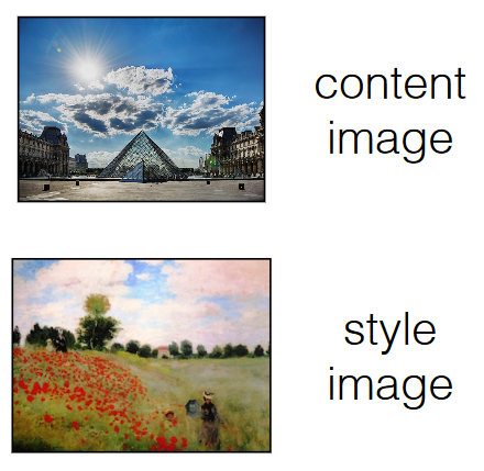
For example, given a photograph of a city as the content image and a painting by Van Gogh as the style image, the algorithm generates a new picture that depicts the city in Van Gogh’s brushstroke and color palette.
Data
-
Unlike supervised learning tasks, style transfer does not require labeled datasets.
-
Only two images are needed:
- a content image (C) – whose structure and layout we want to preserve,
- a style image (S) – whose artistic qualities we want to transfer.
-
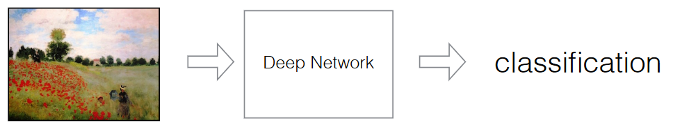
The following figure shows an example of a content image and a style image provided as inputs.
-
The following figure shows the input images for neural style transfer: the left image provides the structural content, and the right image defines the artistic style.
-
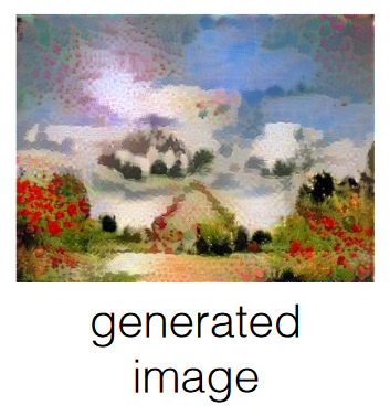
The result is a generated image (G) that combines them.
-
The following figure shows an example of a generated image where the content has been repainted using the artistic style of the chosen style image.
Input and output
- Input: pair \((C, S)\), the content and style images.
- Output: generated image \(G\), optimized to minimize both a content loss and a style loss.
Architecture
- Neural style transfer relies on a pretrained convolutional neural network (CNN), usually trained on ImageNet.
-
CNNs naturally separate different levels of information:
- early layers detect low-level features like edges, gradients, and colors,
- intermediate layers capture textures and shapes,
- deeper layers capture high-level abstractions like objects and scenes.
- The following figure shows how pretrained CNNs can disentangle content (structural information) and style (texture correlations) across different layers of the network.
-
This separation is the key insight behind style transfer:
- content is encoded in deeper feature maps,
- style is encoded by feature correlations, represented using a Gram matrix.
Loss function
-
The optimization objective balances two terms:
\[L(G) = \alpha L_{\text{content}}(C, G) + \beta L_{\text{style}}(S, G)\]- where \(\alpha\) and \(\beta\) are hyperparameters that control the tradeoff.
-
Content loss: ensures that generated image \(G\) preserves the structure of content image \(C\).
\[L_{\text{content}}(C, G) = \| F^l(C) - F^l(G) \|_2^2\]- where \(F^l(X)\) is the feature representation of image \(X\) at layer \(l\).
-
Style loss: ensures that \(G\) mimics the textures of style image \(S\). It is computed using Gram matrices of feature maps:
\[G_{ij}^l(X) = \sum_k F_{ik}^l(X) F_{jk}^l(X)\] \[L_{\text{style}}(S, G) = \sum_l w_l \| G^l(S) - G^l(G) \|_F^2\]- where \(w_l\) are weights controlling each layer’s contribution.
Optimization process
-
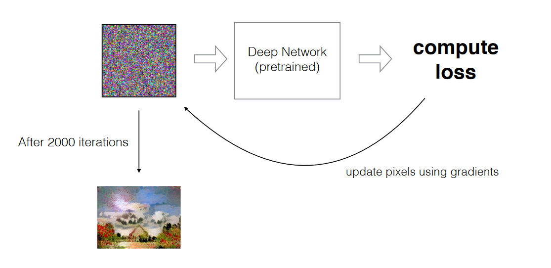
Neural style transfer does not update the CNN weights. Instead, it updates the pixels of \(G\) iteratively:
- Initialize \(G\) as either random noise or a copy of \(C\).
- Forward propagate \(G\) through the pretrained CNN.
- Compute content and style losses.
- Backpropagate the gradients to update pixel values of \(G\).
- Repeat until convergence.
-
The following figure illustrates the final architecture of the NST pipeline, where gradients flow back into the generated image instead of into network weights.
Reference
- Neural style transfer was first proposed in Gatys et al., 2015, titled A Neural Algorithm of Artistic Style.
-
This paper demonstrated that:
- content and style are encoded separately in CNN features,
- optimization over the input image itself can generate high-quality stylized outputs,
- even shallow networks are sufficient to capture artistic styles convincingly.
Trigger word detection
- Trigger word detection is a critical application in speech-based AI systems, particularly for voice assistants such as Siri, Alexa, and Google Assistant. These systems continuously listen for a specific wake word or trigger phrase (e.g., “Hey Siri”, “OK Google”, “Alexa”) before activating more complex functions.
-
The technical challenge lies in designing a model that can:
- detect the trigger word reliably across different accents, speaking speeds, and noisy environments,
- ignore all other sounds such as background noise, music, or irrelevant speech,
- operate in real time with low latency and limited computational resources.
Data
-
To train such a system, we require a dataset of audio clips containing both positive samples (clips with the trigger word) and negative samples (clips without it).
-
Collecting natural data is expensive, so a synthetic data generation pipeline is often used:
- Record independent samples of positive trigger words, negative words, and background noise.
- Overlay trigger words and negatives onto background noise at random times.
- Generate labels automatically, by marking the positions in time where the trigger word occurs.
-
This approach creates a virtually unlimited dataset, while ensuring accurate labeling without manual intervention.
Input
- The model input is typically a 10-second audio clip.
-
Instead of raw waveforms, the audio is transformed into a spectrogram representation — a 2D matrix encoding the intensity of frequencies over time.
- Rows represent frequency bins.
- Columns represent time slices.
- Each value encodes the energy level at that frequency-time point.
- This representation makes speech patterns easier for a neural network to analyze.
Output strategies
-
There are several possible ways to define the output labels for training:
-
Binary classification at the clip level:
- The model outputs a single prediction per 10-second clip.
- 1 if the trigger word appears anywhere, 0 otherwise.
- Limitation: requires huge datasets and ignores the temporal location of the word.
-
Single positive pulse:
- The model outputs a sequence of 0’s with a single 1 at the position where the trigger word starts.
- This provides temporal localization but is fragile, as only one exact frame is positive.
-
Extended pulse (preferred):
- Instead of a single 1, the model outputs a short sequence of consecutive 1’s spanning the trigger word.
- This reduces label sparsity and improves robustness.
-
-
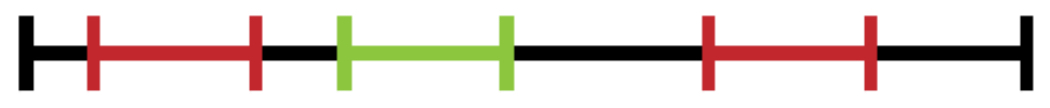
The following figure illustrates trigger word labeling in audio clips: the extended positive pulse during the trigger word ensures stable training and detection. Green segments mark the trigger word, red mark non-trigger words, and black mark silence.
Architecture
-
Since audio is sequential, the natural choice of model is a Recurrent Neural Network (RNN) or its variants:
- LSTMs (Long Short-Term Memory) — handle long-term dependencies.
- GRUs (Gated Recurrent Units) — simpler and computationally cheaper.
-
More recent approaches also leverage 1D convolutions or transformer-based architectures, but RNNs remain standard for introductory treatments.
-
The spectrogram frames are fed sequentially into the RNN, which outputs a probability at each time step for whether the trigger word is active.
Loss function
-
The task is binary classification at each time step. Hence, the binary cross-entropy loss is used:
\[L = - \frac{1}{T} \sum_{t=1}^{T} \Big[ y_t \log(\hat{y}_t) + (1 - y_t)\log(1 - \hat{y}_t) \Big]\]-
where:
-
\(T\) = total number of time steps,
-
\(y_t \in \{0,1\}\) = true label at time \(t\),
-
\(\hat{y}_t\) = predicted probability at time \(t\).
-
-
By training on many synthetic clips, the model learns to emit high probabilities during trigger words while ignoring background noise and irrelevant speech.
Key challenge: data generation
- In practice, data generation quality often matters more than model architecture.
-
Important strategies include:
- Adding background noise overlays (café chatter, traffic, office sounds).
- Using diverse accents, genders, and speaking speeds.
- Mixing in multiple non-trigger words to improve discrimination.
- Without such careful augmentation, models easily overfit to narrow datasets and fail in real environments.
Deployment considerations
- The trained model must operate on-device for real-time detection.
-
Requirements include:
- Low latency: response within milliseconds.
- Low memory footprint: suitable for embedded systems like smart speakers or smartphones.
- Energy efficiency: continuous listening must not drain the device battery.
- Techniques like quantization, pruning, and knowledge distillation are commonly used to compress models while retaining accuracy.
App implementation
-
Once a deep learning model is trained, the next challenge is deployment: making the model usable in real-world applications. This step is often underestimated in difficulty but is crucial for delivering AI systems to end users.
-
To illustrate, let us consider deploying a cat classifier app. The model has been trained to recognize whether an image contains a cat. Now, we want to integrate this model into a mobile phone application.
Two main deployment strategies
-
There are two primary ways to serve a deep learning model inside an application:
-
Server-based implementation
- The app sends the user’s input (e.g., an image) to a remote server.
- The server hosts the model (both architecture and learned parameters).
-
The server performs inference and sends the prediction back to the device.
-
Advantages:
- The app remains lightweight since the model runs elsewhere.
- Model updates are easy — retraining or swapping the model on the server instantly benefits all users.
-
Disadvantages:
- Requires constant internet connectivity.
- Introduces latency due to network communication.
- Raises concerns about privacy since user data must be sent to external servers.
- The following figure illustrates this pipeline, where the phone app communicates with a cloud server for predictions.

-
On-device implementation
- The entire model (architecture + parameters) is stored directly on the device.
-
Inference runs on the phone’s hardware (CPU, GPU, or specialized accelerators like the Neural Engine in iPhones).
-
Advantages:
- Works offline — no internet connection required.
- Much lower latency since predictions are computed locally.
- Better privacy, as data never leaves the device.
-
Disadvantages:
- Limited by device compute and memory.
- Model updates require app updates or background syncing.
- The following figure illustrates on-device inference, where all processing happens locally without contacting external servers.

-
Tradeoffs in deployment
-
The choice between server-based and on-device deployment depends on the tradeoff between scalability and efficiency:
- Server-based deployment is better for very large models (e.g., billions of parameters in GPT-scale models) or when frequent updates are required.
- On-device deployment is ideal when low latency, offline availability, or data privacy are critical.
-
Many real-world applications use hybrid approaches: lightweight models run on-device for fast responses, while more complex models run in the cloud when needed.
Model optimization for on-device use
-
Deep learning models are often too large or computationally expensive for direct deployment. To make on-device inference feasible, researchers use:
- Quantization: reducing parameter precision from 32-bit floating point to 16-bit or 8-bit integers.
- Pruning: removing unnecessary weights or neurons without significantly reducing accuracy.
- Knowledge distillation: training a smaller “student” model to mimic the behavior of a larger “teacher” model.
- Edge-optimized architectures: designing models specifically for resource-constrained devices, such as MobileNet, SqueezeNet, or EfficientNet.
-
These strategies ensure that even devices with limited compute power (smartphones, IoT devices, smart speakers) can run sophisticated AI models efficiently.
Broader implications
- Deployment bridges the gap between research prototypes and production systems.
- Many promising AI models fail to reach users because they cannot be deployed efficiently.
- This highlights the importance of MLOps (Machine Learning Operations), a discipline that ensures machine learning models are trained, versioned, deployed, and monitored reliably at scale.
Shallow neural networks
-
While much of deep learning today focuses on very deep architectures with dozens or even hundreds of layers, it is essential to begin with the simplest case: shallow neural networks. These networks have only one hidden layer, making them an ideal starting point to understand the fundamental computations of forward propagation, backward propagation, and gradient descent.
-
The intuition is that shallow networks are limited in their representational capacity compared to deep networks, but they still provide a rich enough framework to solve nonlinear problems — and they establish the mathematical machinery we generalize later.
Neural network overview
-
A shallow neural network consists of three main parts:
- Input layer: raw features (e.g., pixel values of an image).
- Hidden layer: intermediate transformations using weights, biases, and nonlinear activations.
- Output layer: produces predictions (e.g., class probabilities).
-
Each layer carries out two fundamental steps:
-
Linear transformation
- For layer \(i\):
- where, \(W^{[i]}\) are the weights, \(b^{[i]}\) is the bias vector, and \(x\) is the input to that layer.
-
Nonlinear activation
\[a^{[i]} = \sigma(z^{[i]})\]- where \(\sigma(\cdot)\) is an activation function such as sigmoid, tanh, or ReLU.
-
-
The combination of these steps allows the network to learn nonlinear decision boundaries, something linear models cannot achieve.
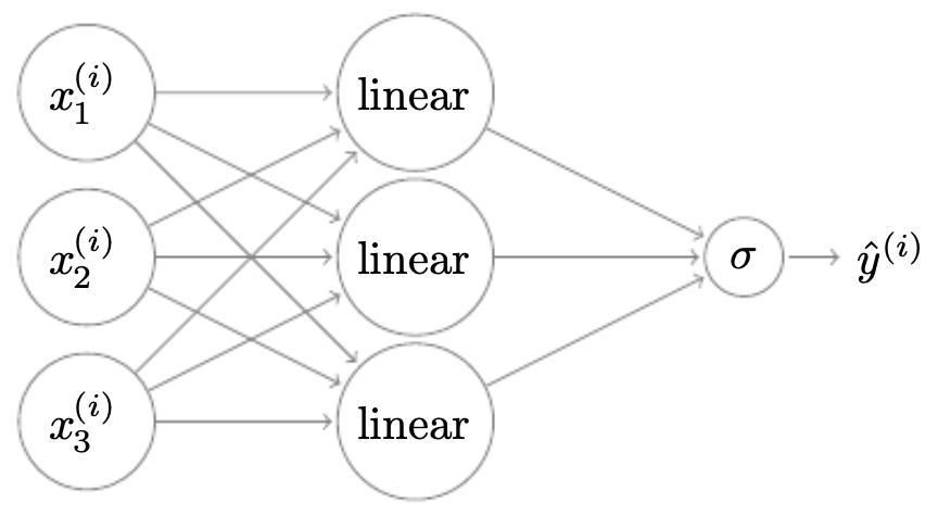
-
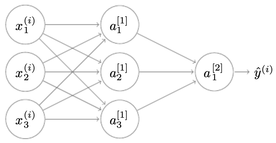
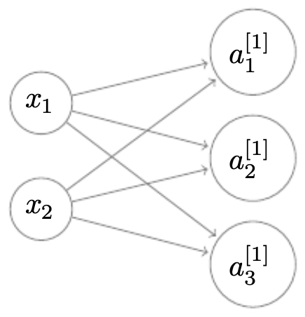
The following figure shows a shallow neural network with one hidden layer of three neurons connected to a single output neuron.
Neural network representations
-
We denote:
- \(a^{[0]} = x\) as the input layer.
- Hidden layers are indexed as \(a^{[1]}\), \(a^{[2]}\), etc.
- The output layer is typically \(a^{[L]}\) where \(L\) is the number of layers.
-
Importantly, when counting network depth, we only count hidden and output layers, not the input layer. Thus, a shallow network with one hidden layer and one output layer is said to be 2 layers deep.
Computing a shallow network’s output
-
Suppose we have a hidden layer with 3 neurons and an output layer with 1 neuron.
-
For the hidden layer:
- For the output layer:
-
The vectorized form of this computation is far more efficient, avoiding explicit loops and allowing GPU acceleration.
-
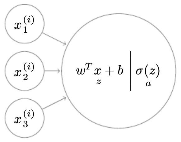
The following figure illustrates how linear activations and nonlinearities are combined neuron by neuron.
Forward propagation across examples
- For multiple training examples (say \(m\) examples), we collect them into a data matrix:
-
Forward propagation can then be written compactly:
\[Z^{[1]} = W^{[1]} X + b^{[1]}, \quad A^{[1]} = \sigma(Z^{[1]})\] \[Z^{[2]} = W^{[2]} A^{[1]} + b^{[2]}, \quad A^{[2]} = \sigma(Z^{[2]})\] -
This vectorization avoids explicit iteration, which is critical for efficiency when \(m\) is in the tens of thousands or higher.
-
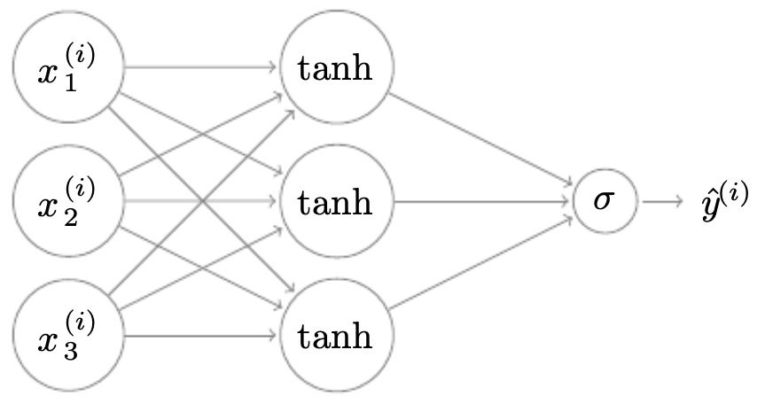
The following figure summarizes the flow of forward propagation in a shallow network.
Activation functions in shallow networks
- The choice of activation function determines the network’s expressiveness and its training dynamics.
-
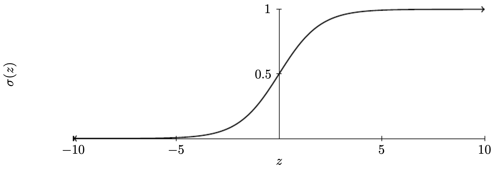
Sigmoid
\[\sigma(z) = \frac{1}{1+e^{-z}}\]-
Maps any input to (0,1). Suitable for binary classification.
-
The following figure shows the sigmoid curve:
-
-
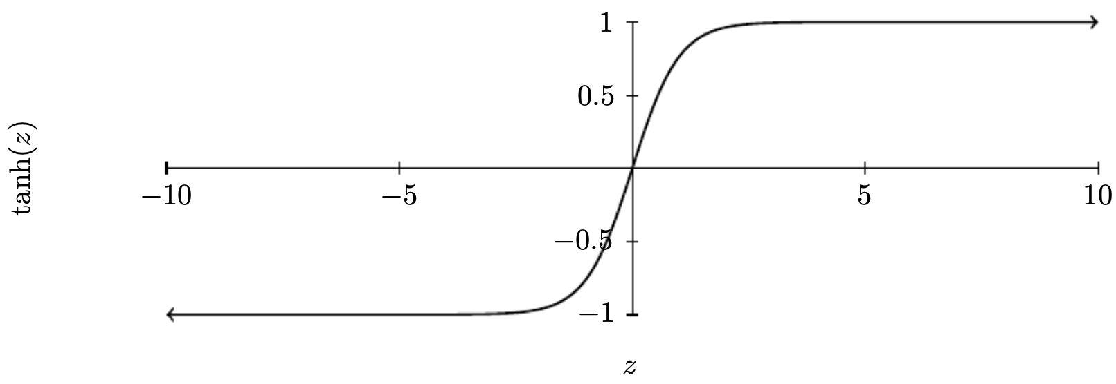
Hyperbolic tangent (tanh)
\[\tanh(z) = \frac{e^z - e^{-z}}{e^z + e^{-z}}\]-
Outputs in (-1,1), centered around zero, often leading to faster convergence.
-
The following figure shows the tanh curve:
-
-
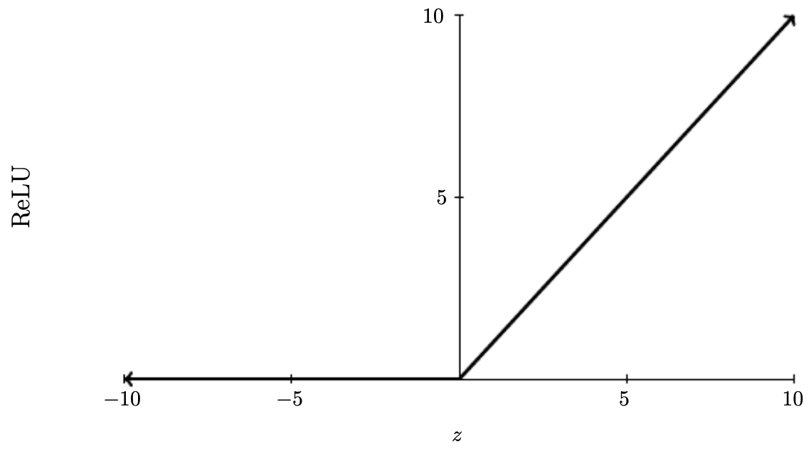
Rectified Linear Unit (ReLU)
\[ReLU(z) = \max(0, z)\]-
Linear for positive inputs, zero otherwise. The most widely used activation in hidden layers today.
-
The following figure shows the ReLU curve:
-
-
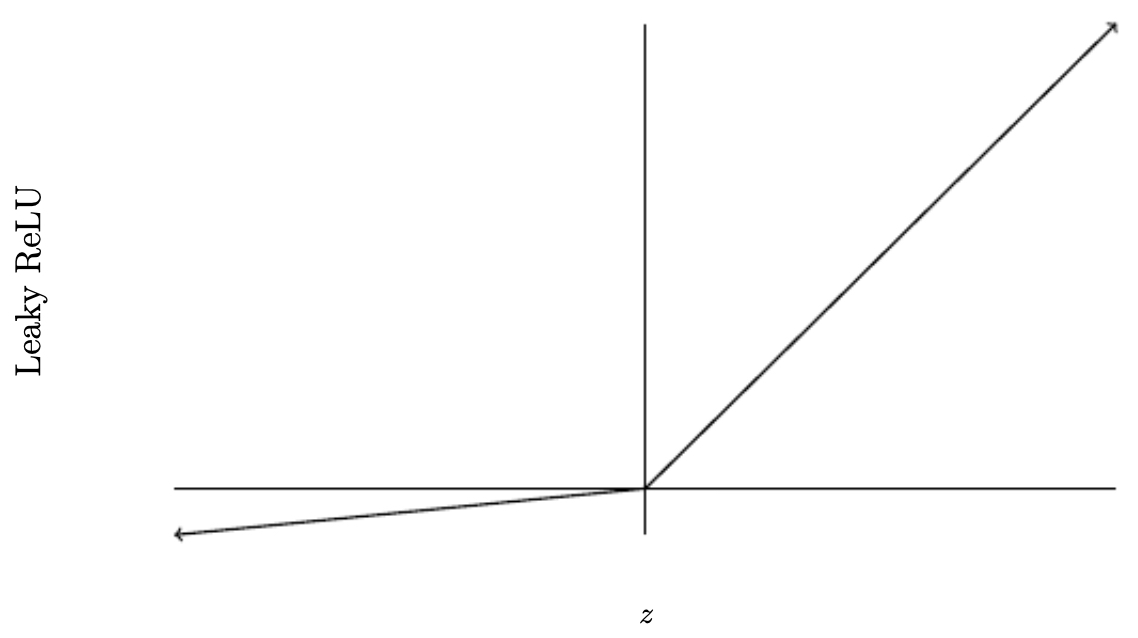
Leaky ReLU
\[LeakyReLU(z) = \max(0.01z, z)\]-
Prevents “dying ReLUs” by allowing a small gradient for negative inputs.
-
The following figure shows the leaky ReLU curve:
-
Why nonlinear activations are essential
- If we only used linear activations, no matter how many layers we stack, the overall function reduces to a single linear transformation. For example:
-
This collapses into:
\[a^{[2]} = (W^{[2]} W^{[1]})x + (W^{[2]}b^{[1]} + b^{[2]})\]- which is still linear. Nonlinear activations are therefore necessary for deep learning to approximate nonlinear decision boundaries.
-
The following figure illustrates how purely linear networks collapse/reduce to a simple logistic regression:
Derivatives of activation functions
When training neural networks, the backpropagation algorithm relies on computing derivatives of activation functions with respect to their inputs. These derivatives determine how errors flow backward through the network and directly affect how parameters (weights and biases) get updated. Understanding them is crucial because poor derivative behavior can lead to training issues such as vanishing or exploding gradients.
Sigmoid derivative
The sigmoid function is:
\[\sigma(z) = \frac{1}{1 + e^{-z}}\]A key property is that its derivative can be written in terms of itself:
\[\sigma'(z) = \sigma(z)(1 - \sigma(z))\]This makes computation efficient, since we already calculate \(\sigma(z)\) during the forward pass and can reuse it during backpropagation.
Limitation: For very large positive or negative values of \(z\), \(\sigma(z)\) saturates near 0 or 1, making \(\sigma'(z)\) close to 0. This is the vanishing gradient problem.
Hyperbolic tangent derivative
- The tanh activation is:
- Its derivative is:
- This derivative also shrinks toward 0 as \(\| z \|\) grows large, which means tanh also suffers from vanishing gradients, though it has the advantage of being zero-centered (unlike sigmoid).
ReLU derivative
- The ReLU activation is:
- Its derivative is simple:
-
At \(z=0\), the derivative is undefined, but in practice it is assigned either 0 or 1 arbitrarily, since this rarely affects performance.
- Strength: ReLU avoids vanishing gradients for positive inputs.
- Weakness: Some neurons may get stuck outputting only 0’s (if their weights push inputs permanently into the negative region). This is called the dying ReLU problem.
Leaky ReLU derivative
- To address dying ReLUs, Leaky ReLU allows a small slope in the negative region:
- Its derivative is:
- This ensures gradients never vanish completely, even for negative inputs.
Why derivatives matter
- If the derivative is too small, learning slows or halts (vanishing gradient problem).
- If the derivative is too large, parameter updates explode, destabilizing training (exploding gradient problem).
-
ReLU and its variants are popular because they preserve strong gradients for positive inputs, making deep networks trainable.
- The following figure illustrates the slope of leaky ReLU in the negative region, which helps prevent neuron “death” by keeping gradients alive, ultimately avoiding vanishing gradients for negative values:
Gradient descent for neural networks
- Training a neural network means adjusting its parameters (weights and biases) so that the network’s predictions align as closely as possible with the true labels. This adjustment is carried out by gradient descent, which uses the derivatives computed during backpropagation to update parameters in the direction that minimizes the loss function.
Cost function
-
For binary classification, the most common cost function is cross-entropy loss (also called logistic loss). Given training set size \(m\), the cost function is:
\[J(W^{[1]}, b^{[1]}, W^{[2]}, b^{[2]}) = \frac{1}{m} \sum_{i=1}^m L(\hat{y}^{(i)}, y^{(i)})\]- … where each individual loss is:
-
where:
- \(y \in \{0,1\}\) is the true label,
- \(\hat{y}\) is the predicted probability from the network’s forward propagation.
-
This formulation penalizes confident wrong predictions very heavily, encouraging the model to refine its estimates.
Gradient descent update rule
-
After computing gradients with respect to each parameter, we update them iteratively. For layer \(\ell\):
\[W^{[\ell]} := W^{[\ell]} - \alpha \, dW^{[\ell]}, \quad b^{[\ell]} := b^{[\ell]} - \alpha \, db^{[\ell]}\]-
where:
- \(\alpha\) is the learning rate (a hyperparameter),
- \(dW^{[\ell]}\) and \(db^{[\ell]}\) are gradients of the cost with respect to parameters \(W^{[\ell]}\) and \(b^{[\ell]}\).
-
-
If \(\alpha\) is too small, training is slow. If it is too large, the algorithm may oscillate and fail to converge.
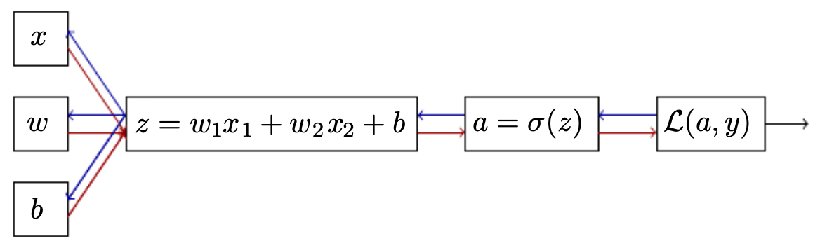
Computational graph perspective
-
It is often helpful to visualize forward and backward propagation as a computational graph, where:
- Forward propagation computes activations moving left to right.
- Backward propagation computes derivatives flowing right to left.
-
The following figure illustrates logistic regression as a computational graph. Red arrows denote forward propagation, while blue arrows denote backward propagation of derivatives:
Two-layer network example
- In a two-layer network, forward propagation computes:
-
During backpropagation, we compute derivatives step by step:
\[dZ^{[2]} = a^{[2]} - y\] \[dW^{[2]} = \frac{1}{m} dZ^{[2]} (a^{[1]})^T, \quad db^{[2]} = \frac{1}{m}\sum dZ^{[2]}\] \[dZ^{[1]} = W^{[2]T} dZ^{[2]} \ast g^{[1]'}(Z^{[1]})\] \[dW^{[1]} = \frac{1}{m} dZ^{[1]} X^T, \quad db^{[1]} = \frac{1}{m}\sum dZ^{[1]}\]- where \(\ast\) denotes elementwise multiplication, and \(g^{[1]'}\) is the derivative of the activation function in layer 1.
-
The following figure shows how forward propagation (top) caches intermediate values, which are later reused for efficient backward propagation (bottom):
Key insights
- Forward propagation computes activations layer by layer.
- Backward propagation computes gradients using cached intermediate variables.
- Gradient descent updates parameters iteratively until the cost converges.
- Together, these steps define the fundamental training loop of neural networks.
Random initialization
-
The initialization of parameters in a neural network is critical. If initialization is done poorly, the network may fail to learn meaningful representations, either because neurons become redundant or because gradients vanish/explode. Initialization strategies are designed to ensure that:
- Neurons learn different features (avoid redundancy).
- Gradients remain in a reasonable range as they propagate forward and backward.
The symmetry breaking problem
- Suppose we initialize the weights in the first layer as:
-
Now imagine that instead of this arbitrary example, we initialize all weights in a layer to the same value (e.g., all zeros or all ones). In that case:
- Each neuron in the same layer receives identical inputs and produces identical outputs.
- Their gradients during backpropagation are also identical.
- Consequently, all neurons evolve in lockstep during training and never diverge to learn different features.
-
This phenomenon is called symmetry, and it makes multiple neurons completely redundant. To break symmetry, weights must be initialized randomly.
Random small weights
-
A simple strategy is to draw weights from a Gaussian distribution and scale them by a small factor, for example:
\[W^{[1]} = 0.01 \times \text{np.random.randn}(2, 2)\]- where, the factor 0.01 ensures that initial weights are small. This matters because activation functions such as sigmoid or tanh saturate when inputs are very large or very small, producing gradients close to zero. Starting with small values keeps activations in the sensitive, non-saturated region, allowing learning to proceed efficiently.
-
Biases, however, can safely be initialized to zero:
- This does not create symmetry problems, because biases shift activations but do not define distinct features in the same way as weights.
Modern initialization strategies
-
While “small random weights” is a good starting point, research has revealed better scaling rules tailored to specific activation functions:
-
Xavier initialization (Glorot & Bengio, 2010)
- Designed for sigmoid and tanh activations.
- Weights are drawn from a distribution with variance proportional to \(\frac{1}{n_{\text{in}}}\), where \(n_{\text{in}}\) is the number of inputs to the neuron.
- Ensures that the variance of activations is stable across layers.
-
He initialization (He et al., 2015)
- Designed for ReLU activations.
- Weights are drawn with variance proportional to \(\frac{2}{n_{\text{in}}}\).
- Prevents vanishing gradients by keeping activations “alive” through deeper networks.
-
-
These initialization schemes are now standard practice in modern deep learning libraries (TensorFlow, PyTorch, Keras, etc.).
Why initialization matters
-
If initialization is too small:
- Signals shrink as they propagate forward.
- Gradients shrink as they propagate backward.
- The network suffers from the vanishing gradient problem.
-
If initialization is too large:
- Signals explode as they propagate forward.
- Gradients explode as they propagate backward.
- Training becomes unstable and may diverge.
-
Proper initialization helps maintain a healthy signal flow through the network, keeping both activations and gradients within a useful range.
Visualization of initialization effects
- The following figure illustrates the consequences of different initialization strategies. With poor initialization, neurons behave identically, failing to learn diverse features. With random initialization, symmetry is broken, allowing each neuron to capture distinct aspects of the data.
Deep neural networks
-
So far, we have examined shallow networks (with one or two hidden layers). While these are useful for building intuition, modern breakthroughs in artificial intelligence have relied on deep neural networks (DNNs) — architectures that stack many hidden layers to extract increasingly abstract and complex representations of data.
-
Deep networks provide expressive power: they can represent complicated functions with fewer units than shallow ones. However, they also introduce new challenges, including vanishing gradients, exploding gradients, and optimization difficulties.
Notation
-
We formalize deep networks with the following notation:
- \(L\): total number of layers in the network.
- \(n^{[\ell]}\): number of neurons in layer \(\ell\).
- \(a^{[\ell]}\): activations (outputs) of layer \(\ell\).
- \(z^{[\ell]}\): pre-activation values in layer \(\ell\), computed as the linear combination before applying the activation.
- \(W^{[\ell]}, b^{[\ell]}\): weights and biases associated with layer \(\ell\).
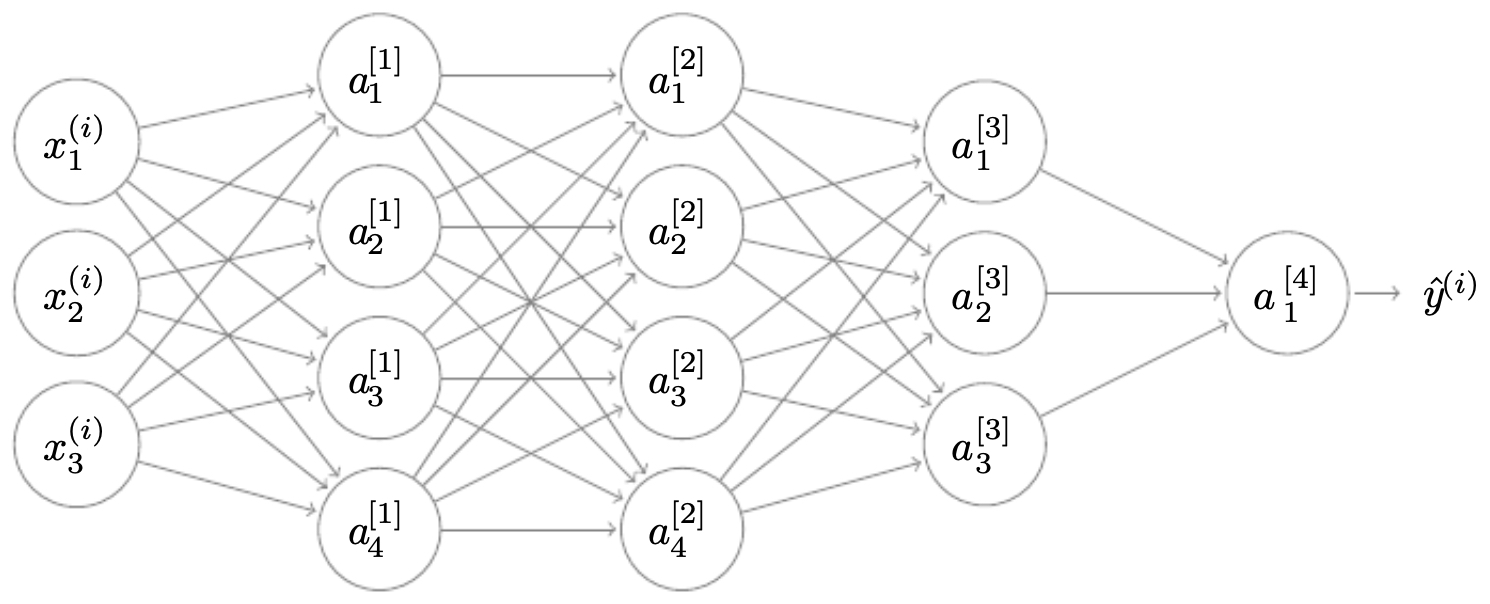
-
For example, in the following figure, we see a deep network with 4 layers, each with a different number of units:
-
The following figure shows a schematic of a 4-layer neural network with varying widths across layers, illustrating how input flows through multiple transformations.
Forward propagation in deep networks
-
Generalizing from shallow networks, forward propagation in a deep network for a single training example is:
\[z^{[\ell]} = W^{[\ell]} a^{[\ell-1]} + b^{[\ell]}, \quad a^{[\ell]} = g^{[\ell]}(z^{[\ell]})\]- … for \(\ell = 1, 2, \dots, L\), where \(g^{[\ell]}\) is the activation function in layer \(\ell\).
-
In matrix form (for all \(m\) training examples at once):
\[Z^{[\ell]} = W^{[\ell]} A^{[\ell-1]} + b^{[\ell]}, \quad A^{[\ell]} = g^{[\ell]}(Z^{[\ell]})\]- where \(A^{[0]} = X\), the input data matrix.
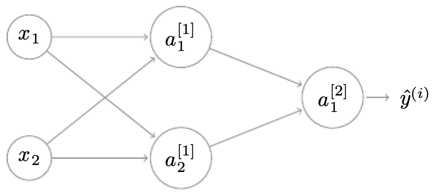
Dimension consistency
-
One of the most common pitfalls in building deep networks is mismatched dimensions. To keep track:
-
If \(a^{[\ell-1]} \in \mathbb{R}^{n^{[\ell-1]} \times m}\), then:
- \[W^{[\ell]} \in \mathbb{R}^{n^{[\ell]} \times n^{[\ell-1]}}\]
- \[b^{[\ell]} \in \mathbb{R}^{n^{[\ell]} \times 1}\]
- \[z^{[\ell]}, a^{[\ell]} \in \mathbb{R}^{n^{[\ell]} \times m}\]
-
-
The following figure shows how matrix dimensions propagate correctly through a neural network with 2 inputs and 3 hidden units.
Why deeper representations?
-
The power of deep networks lies in their ability to extract hierarchical features:
- Early layers capture low-level patterns, such as edges or corners.
- Intermediate layers capture parts of objects, such as eyes, ears, or textures.
- Later layers capture whole objects, such as faces, animals, or cars.
-
This hierarchy mirrors the organization of the human visual cortex, where simple features are detected early and complex concepts emerge later.
-
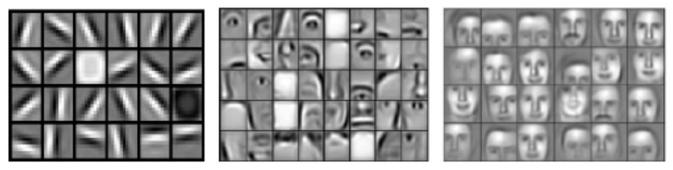
The following figures show how deeper layers progressively detect more complex features, from edges to shapes to objects. (Top) The hierarchical nature of feature extraction in deep networks is shown, from low-level edges to higher-level parts. (Bottom) Continuation of the hierarchy visualization, showing how networks transition from detecting simple curves to semantically meaningful structures.
Example: logic trees
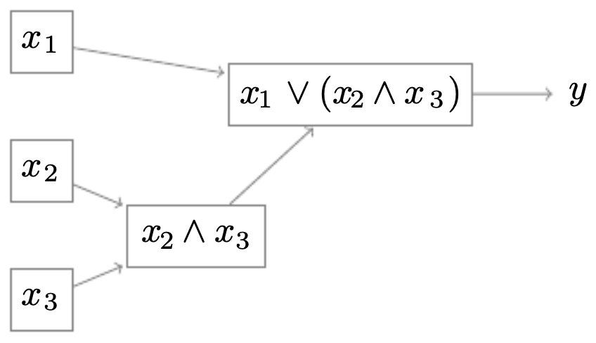
- To illustrate why deep networks are more efficient, consider the Boolean function:
-
A deep tree can represent this compactly with few nodes. A shallow tree, however, needs exponentially many nodes to enumerate all possible combinations of \((x_1, x_2, x_3)\).
-
The following figures compare these two representations. (Top) A deep logic tree that represents the Boolean function \(y = x_1 \lor (x_2 \land x_3)\) with far fewer nodes. (Bottom) A shallow logic tree that needs exponentially more nodes to represent the same Boolean function, since it must test every combination explicitly.
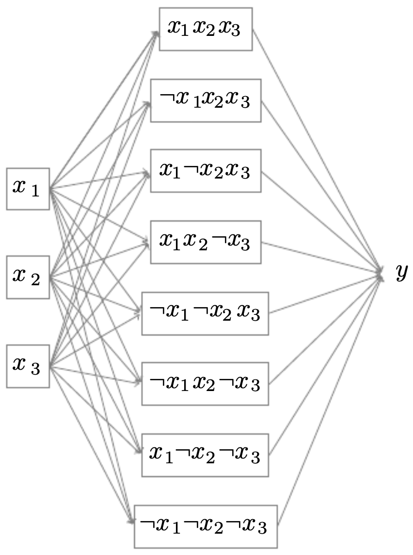
- This demonstrates the expressive efficiency of deep architectures: they can represent complex functions more compactly than shallow ones.
Forward and backward propagation in deep networks
-
Training deep neural networks follows the same fundamental principles as shallow ones, but the process scales across many more layers. The two central phases are:
- Forward propagation: computing activations layer by layer.
- Backward propagation: computing gradients with respect to each parameter using the chain rule of calculus.
-
To manage this efficiently, intermediate values (such as \(z^{[\ell]}\) and \(a^{[\ell]}\)) are cached during the forward pass and reused during backpropagation.
Forward propagation
-
For a given layer \(\ell\):
\[z^{[\ell]} = W^{[\ell]} a^{[\ell-1]} + b^{[\ell]}\] \[a^{[\ell]} = g^{[\ell]}(z^{[\ell]})\]-
where:
- \(W^{[\ell]}\) and \(b^{[\ell]}\) are the parameters of the layer,
- \(g^{[\ell]}\) is the activation function (sigmoid, ReLU, tanh, etc.),
- \(a^{[\ell-1]}\) is the output of the previous layer (or the input \(X\) when \(\ell = 1\)).
-
-
Forward propagation proceeds sequentially from the first layer through the final layer \(L\), producing predictions \(\hat{y} = a^{[L]}\).
Backward propagation
-
Backward propagation applies the chain rule to compute how the loss depends on each parameter.
-
Given the derivative of the cost with respect to activations at layer \(\ell\), denoted \(dA^{[\ell]}\), we compute:
\[dZ^{[\ell]} = dA^{[\ell]} \ast g^{[\ell]'}(Z^{[\ell]})\] \[dW^{[\ell]} = \frac{1}{m} dZ^{[\ell]} (A^{[\ell-1]})^T\] \[db^{[\ell]} = \frac{1}{m} \sum dZ^{[\ell]}\] \[dA^{[\ell-1]} = (W^{[\ell]})^T dZ^{[\ell]}\]- where \(\ast\) denotes elementwise multiplication, and \(g^{[\ell]'}\) is the derivative of the activation function at that layer.
-
Backward propagation runs in reverse order, starting from the output layer \(L\) and moving back to layer 1.
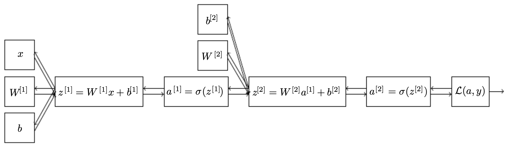
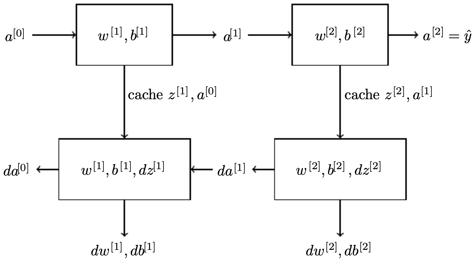
Two-layer example
-
To solidify the idea, consider a 2-layer network:
-
Forward pass:
\[z^{[1]} = W^{[1]}x + b^{[1]}, \quad a^{[1]} = g^{[1]}(z^{[1]})\] \[z^{[2]} = W^{[2]}a^{[1]} + b^{[2]}, \quad a^{[2]} = g^{[2]}(z^{[2]})\] -
Backward pass:
\[dZ^{[2]} = a^{[2]} - y\] \[dW^{[2]} = \frac{1}{m} dZ^{[2]} (a^{[1]})^T, \quad db^{[2]} = \frac{1}{m} \sum dZ^{[2]}\] \[dZ^{[1]} = (W^{[2]})^T dZ^{[2]} \ast g^{[1]'}(Z^{[1]})\] \[dW^{[1]} = \frac{1}{m} dZ^{[1]} X^T, \quad db^{[1]} = \frac{1}{m} \sum dZ^{[1]}\] -
The following figure illustrates this, with forward propagation moving across the top path and backward propagation flowing along the bottom path in a two-layer network:
Generalization to \(L\) layers
-
For a deep network with \(L\) layers:
- Forward propagation runs from layer 1 to \(L\), sequentially computing \(z^{[\ell]}\) and \(a^{[\ell]}\).
- Backward propagation runs from layer \(L\) back to 1, computing gradients layer by layer.
-
This recursive structure makes implementations modular: in code, we define one forward function and one backward function per layer type, then loop through them during training.
Parameters vs. Hyperparameters
- When training deep neural networks, one of the most important distinctions to keep in mind is the difference between parameters and hyperparameters. Although the two terms are sometimes confused, they play very different roles in the training process.
Parameters
-
Parameters are the quantities that the neural network learns automatically from the data during training. They define how the network processes inputs and produces outputs.
- Weights \(W^{[\ell]}\): the coefficients that scale and combine the inputs at layer \(\ell\).
-
Biases \(b^{[\ell]}\): offsets that shift the activations at layer \(\ell\).
-
These are updated iteratively by gradient descent (or one of its variants, such as Adam or RMSProp).
-
Mathematically, for a single layer:
\[z^{[\ell]} = W^{[\ell]} a^{[\ell-1]} + b^{[\ell]}, \quad a^{[\ell]} = g^{[\ell]}(z^{[\ell]})\]- where, \(W^{[\ell]}\) and \(b^{[\ell]}\) are the parameters.
- During training, each forward and backward propagation step adjusts these values so that predictions \(\hat{y}\) better match the true labels \(y\).
Hyperparameters
-
Hyperparameters, by contrast, are design choices made before training begins. They are not learned by the network; instead, they determine how the learning process itself unfolds.
-
Examples of hyperparameters include:
- Learning rate \(\alpha\): how big each update step is in gradient descent.
- Number of layers \(L\).
- Number of units per layer \(n^{[\ell]}\).
- Choice of activation functions (ReLU, sigmoid, tanh, etc.).
- Batch size: number of training examples processed before updating weights.
- Number of epochs: how many passes are made over the training dataset.
- Optimization algorithm (SGD, Adam, RMSProp).
- Regularization strength (e.g., L2 penalty \(\lambda\), dropout rate).
-
Unlike parameters, these are not derived from data but chosen by the researcher or practitioner.
Tuning hyperparameters
-
Since no closed-form solution exists for the “best” hyperparameters, they must be tuned experimentally. Common approaches include:
- Grid search: exhaustively trying combinations of hyperparameter values.
- Random search: sampling hyperparameters from predefined distributions — often more efficient than grid search (Bergstra & Bengio, 2012).
- Bayesian optimization: modeling the hyperparameter space probabilistically to find promising regions.
- Automated ML (AutoML): modern frameworks that automate hyperparameter search using advanced algorithms.
-
Good hyperparameter tuning can often make a much larger difference than small tweaks to the model architecture.
Takeaways
- Parameters: learned during training (weights, biases).
- Hyperparameters: chosen manually (learning rate, architecture, optimizer, etc.).
- Parameters define the function the network learns, while hyperparameters define the process by which it learns.
Connection to the Brain
- The term neural network originates from early attempts to mimic the biological brain. While the resemblance is mostly metaphorical today, the analogy still provides helpful intuition. Modern artificial neural networks borrow inspiration from neuroscience, but the actual mechanisms are highly simplified mathematical abstractions.
Biological neurons
-
A biological neuron consists of three main components:
- Dendrites: receive incoming signals (electrical impulses) from other neurons.
- Cell body (soma): integrates the incoming signals. If the combined signal exceeds a threshold, the neuron “fires.”
- Axon: transmits the output signal to other connected neurons.
-
The process is all-or-nothing: a neuron either fires or does not, depending on whether the inputs cross a threshold. Synaptic plasticity — the strengthening or weakening of synapses based on experience — is thought to underlie learning in the brain.
Artificial neurons
- Artificial neurons are simplified mathematical models designed to approximate this process:
- Inputs: analogous to dendrites, the values from the previous layer \(a^{[\ell-1]}\).
- Weights \(W^{[\ell]}\): analogous to synaptic strengths.
- Biases \(b^{[\ell]}\): analogous to neuron thresholds.
-
Activation function \(g^{[\ell]}(\cdot)\): introduces nonlinearity, loosely inspired by the firing behavior of neurons.
- Unlike the brain, artificial neurons do not “spike” — they output continuous values between 0 and 1 (sigmoid), between -1 and 1 (tanh), or any non-negative value (ReLU).
Key differences
-
Despite the naming similarities, important distinctions exist between artificial and biological networks:
-
Learning mechanism:
- The brain learns through mechanisms such as Hebbian plasticity (“neurons that fire together, wire together”).
- Artificial networks learn via backpropagation, a purely mathematical algorithm that computes derivatives and updates weights using gradient descent. No evidence suggests the brain implements anything like backpropagation.
-
Signal transmission:
- Biological neurons communicate through electrochemical spikes.
- Artificial neurons pass continuous real-valued activations.
-
Scale and connectivity:
- The human brain has roughly 86 billion neurons, each connected to thousands of others.
- Artificial networks are far smaller, with far simpler connectivity patterns.
-
The loose analogy
-
Although the mechanisms differ, both biological and artificial networks share some conceptual similarities:
- Networks consist of interconnected units passing signals.
-
Layers of processing yield hierarchical representations:
- In vision, biological neurons progress from detecting edges (retina, early visual cortex) to complex objects (higher visual cortex).
- In artificial CNNs, early layers detect edges, mid-level layers detect textures and parts, and later layers detect whole objects.
-
Thus, neural networks are brain-inspired, not brain-replicating. They borrow terminology and ideas from neuroscience but are primarily engineering constructs optimized for computation.
Takeaway
- Neural networks are best understood as powerful function approximators, not accurate models of cognition. They draw inspiration from neuroscience but follow fundamentally different principles. As Yann LeCun has emphasized, modern deep learning is an engineering tool first and foremost, rather than a direct attempt to simulate the brain.
Citation
If you found our work useful, please cite it as:
@article{Chadha2020NeuralNetworks,
  title   = {Neural Networks},
  author  = {Chadha, Aman},
  journal = {Distilled Notes for Stanford CS230: Deep Learning},
  year    = {2020},
  note    = {\url{https://aman.ai}}
}