CS230 • Introduction to Deep Learning
- Overview
- The Growth of Deep Learning Research
- Why Now?
- Deep Learning
- What is a Neural Network?
- Applications of Neural Networks
- Sign Language Detection**
- The Happy House (Sentiment-based Filtering)**
- Face Recognition**
- Object Detection for Autonomous Driving**
- Sports Analytics: Goalkeeper Shoot Prediction**
- Art Generation (Neural Style Transfer)**
- Music Generation**
- Text Generation**
- Sentiment Analysis and Emoji Prediction**
- Machine Translation**
- Trigger Word Detection**
- Architectures of Neural Networks
- Logistic Regression as a Neural Network
- Python and Vectorization
- Citation
Overview
-
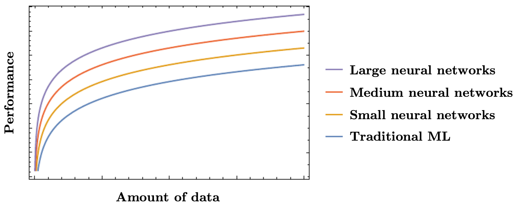
The gist of deep learning, and the algorithms behind it, have been around for decades. However, we saw that as we started to add data to neural networks, they began to perform much better than traditional machine learning algorithms. With advances in GPU computing and the vast amount of data we now have available, training larger neural networks has become easier than ever before. With more data, larger neural networks have been shown to outperform all other machine learning algorithms. To make this concrete, consider the empirical “scaling law” trend: when model capacity (parameters), dataset size, and compute are increased in tandem, held-out error typically decreases smoothly on log–log axes. This is not because large models merely memorize; rather, their higher capacity allows them to fit complex functions while regularization, data augmentation, and optimization schedules (e.g., learning-rate warmup and cosine decay) keep generalization in check.
-
The following figure shows how larger neural networks, given sufficient data, outperform both smaller networks and traditional machine learning methods. Read the horizontal axis as the amount of high-quality data available and the vertical axis as achievable test performance. In low-data regimes, classical methods or small nets can be competitive; as data grows, overparameterized nets unlock lower error because they can represent richer hypotheses without hitting an approximation ceiling.
-
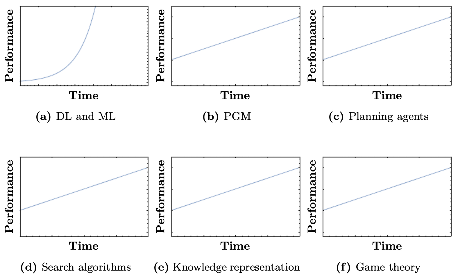
Artificial intelligence (AI) can be broken down into several subfields: deep learning (DL), machine learning (ML), probabilistic graphical models (PGM), planning agents, search algorithms, knowledge representation (KR), and game theory. Among these, the only subfields that have dramatically improved in performance in recent years are deep learning and machine learning. A key reason is end-to-end differentiability paired with massive supervision or self-supervision: gradients provide a scalable learning signal that can be propagated through very large parametric systems, whereas many symbolic approaches require brittle hand-crafted rules or struggle to exploit raw, uncurated data at scale.
-
The following figure illustrates how the performance of DL and ML has exploded relative to other subfields of AI such as PGMs, planning agents, search algorithms, knowledge representation, and game theory. Interpreting the figure, you can think of “performance” as a proxy for benchmark accuracy or capability across vision, language, and speech tasks; DL/ML curves rise steeply as compute and data accelerate, while the others improve more modestly because their methods don’t directly capitalize on these two levers.
The Growth of Deep Learning Research
-
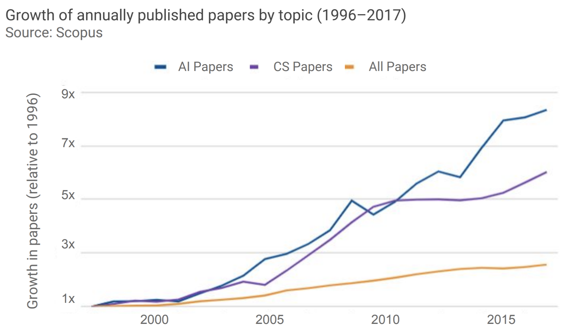
The rise of artificial intelligence is not confined to computer science departments. The number of annually published papers in AI has outpaced that of computer science overall, meaning researchers from other fields such as physics, chemistry, astronomy, and material science are actively contributing to AI. This growth signals that AI is not only a computational tool but also a scientific instrument: physicists use it for particle detection, chemists for molecular property prediction, and astronomers for telescope data analysis.
-
The following figure shows the rapid increase of AI-related papers, outpacing general computer science publications. Notice how the slope for AI accelerates sharply around the early 2010s, coinciding with breakthroughs like ImageNet classification with deep CNNs. The data suggests an exponential rise in interest as both academia and industry recognized the transformative potential of deep learning.
-
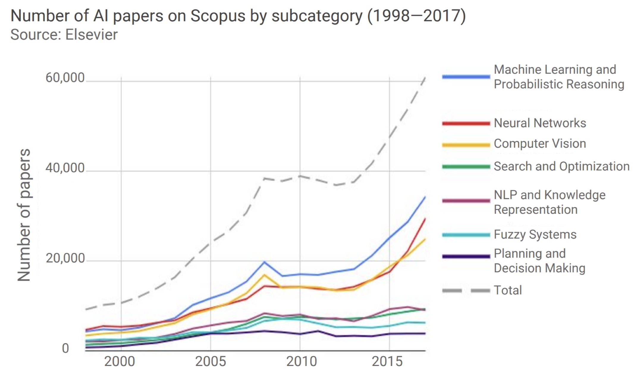
The keyword “Neural Network” has also seen an exponential rise in research publications, particularly in the 2010s. Early mentions were sparse through the 1980s and 1990s during the so-called “AI winters,” but the advent of powerful GPUs and benchmark successes reignited the field.
-
The following figure illustrates the rapid increase in papers published with the keyword “Neural Network,” demonstrating the surge of interest in deep learning. Each uptick represents thousands of new contributions spanning topics from fundamental optimization to applied domains like medical imaging and natural language processing.
-
Between 2014 and 2017, the number of Scopus papers on Neural Networks had a compound annual growth rate of 37%. This surge was especially visible in machine learning and computer vision research. Deep learning has since reshaped the frontiers of machine learning, natural language processing, and computer vision, with models like CNNs, RNNs, and Transformers setting new state-of-the-art benchmarks. Importantly, this surge has also spread to interdisciplinary applications, accelerating scientific discovery in genomics, drug discovery, and climate modeling.
-
Applications of deep learning have already permeated our everyday lives. Conversational assistants such as Siri or Alexa, face verification for unlocking phones, self-driving car perception systems, itinerary mapping, sentiment analysis, and machine translation all rely on deep learning. The broader takeaway is that the research explosion directly fuels the technologies we interact with daily: each paper contributes to an incremental advance that aggregates into systems capable of human-like perception, reasoning, and interaction.
Why Now?
-
The boom of AI in the last decade is largely driven by three reinforcing factors:
-
Digitization: An explosion of available data due to sensors, online behavior, digital communication, and large-scale datasets. Smartphones, IoT devices, and social platforms generate billions of images, videos, and text snippets daily. This unprecedented supply of labeled and unlabeled data provides the raw material for training deep models at scale. Without this digitization, even the best algorithms would be starved of fuel.
-
Computation: Advances in GPUs, TPUs, and distributed training have enabled efficient large-scale optimization. Specialized hardware allows massively parallelized linear algebra operations, which are the backbone of deep learning (matrix multiplications, convolutions, tensor contractions). Multi-GPU and cloud-based training strategies also make it possible to train models with billions of parameters in days rather than months.
-
Algorithms: Advances in neural architectures (e.g., CNNs for vision, RNNs for sequential modeling, Transformers for attention-based learning) and training techniques (e.g., batch normalization, dropout, residual connections, adaptive optimizers like Adam) have overcome earlier obstacles such as vanishing gradients and unstable training. These innovations have made networks deeper, more expressive, and easier to optimize.
-
-
At its core, machine learning is about learning a function that maps data to labels and then using that function to make predictions on new data. Classical models such as linear regression fit hyperplanes in feature space but are limited in expressive power. For example, logistic regression can separate data with linear decision boundaries but struggles when features interact in complex, nonlinear ways.
-
Deep learning scales to massive data by leveraging multiple nonlinear transformations and layered representations. Each layer of a neural network transforms raw inputs into progressively more abstract features. Early layers may detect edges in images or phonemes in speech, while later layers detect object categories or semantic meaning. This hierarchical structure mirrors how humans interpret sensory input, enabling deep networks to handle problems previously thought intractable for machines.
-
The key insight of this section is that “Why now?” is not explained by any single factor. Instead, the synergy of big data, affordable compute, and algorithmic breakthroughs unlocked the dormant potential of neural networks that had been studied for decades. What seemed impractical in the 1980s and 1990s became state-of-the-art in the 2010s and continues to accelerate into the present.
Deep Learning
What is a Neural Network?
-
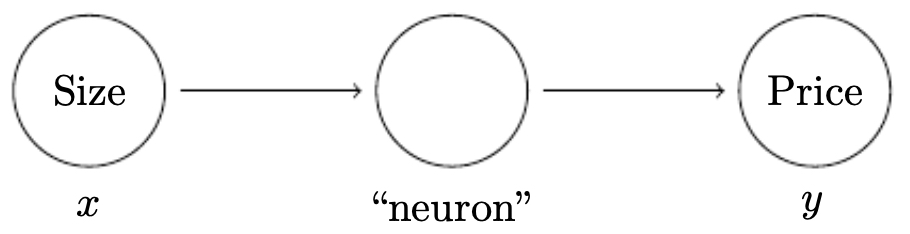
The aim of a neural network is to learn representations that best predict the output \(y\), given a set of features as the input \(x\). In essence, a neural network learns a mapping function \(f_\Theta(x) \rightarrow y\), where \(\Theta\) represents the parameters (weights and biases) optimized during training.
-
The following figure shows the simplest possible neural network, with a single input feature (size of a home) and a single output (price). This basic setup resembles linear regression: the neuron learns a weighted sum of the input and passes it through an activation function to produce the output.
-
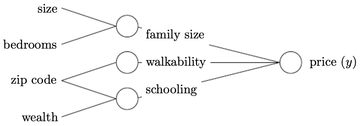
Here, the neuron is the component that tries to learn a function mapping \(x \rightarrow y\). Because this example only has one neuron, it is the simplest case. However, neural networks derive their power from scaling this idea. We can build more complex neural networks by stacking neurons. For example, if instead of just the size of a home we also had the number of bedrooms, the zip code, or local wealth indicators, we would represent these as additional inputs to the network. Each input is assigned its own weight, and the neuron combines them to produce a prediction.
-
The following figure illustrates how intermediate connections between inputs may themselves encode useful features (such as family size, walkability, and schooling). In practice, these hidden neurons compute nonlinear combinations of raw features, making the learned representation more powerful than direct input-output mapping.
-
Neural networks work well because we do not need to explicitly hand-engineer these intermediate values; instead, they are learned automatically during training. Hidden layers progressively refine raw input into useful abstractions. When all inputs in one layer are connected to all outputs of the next, we call this a fully connected (dense) layer.
-
The following figure shows a standard neural network consisting of an input layer, hidden layer, and output layer, all fully connected. This diagram captures the fundamental structure underlying many architectures: layers of interconnected neurons that learn distributed representations.
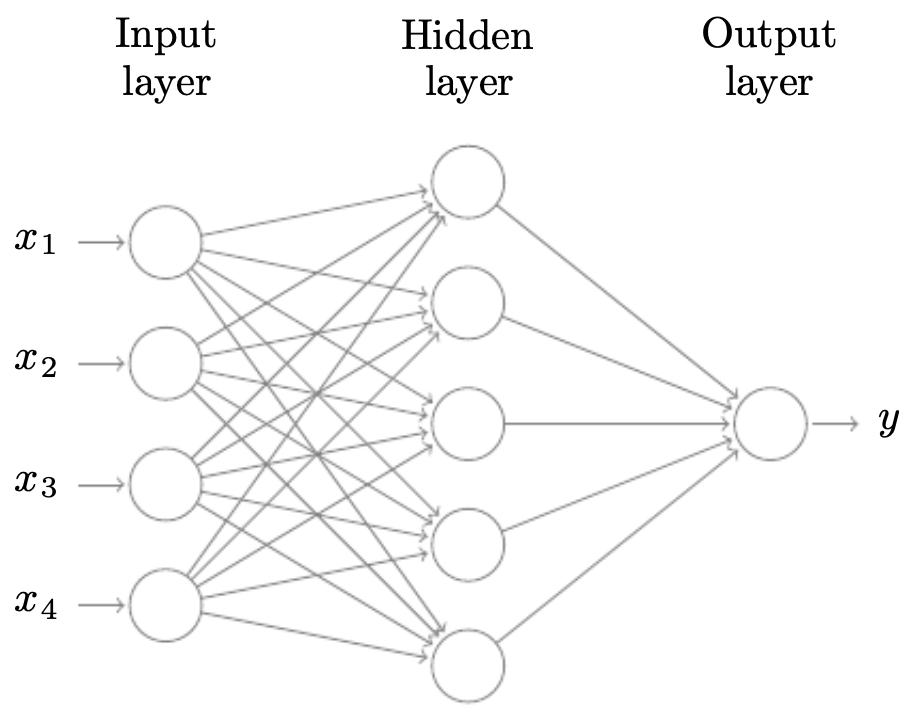
- By stacking many such layers, neural networks can approximate highly complex functions, a property formalized by the Universal Approximation Theorem. The expressiveness grows with depth and width, enabling models to capture hierarchical structure in data—from pixels to edges to objects in images, or from characters to words to semantic meaning in text.
Applications of Neural Networks
- Neural networks are versatile because they can approximate highly complex functions, making them applicable to a wide range of real-world tasks. Almost all of the hype around machine learning has centered around supervised learning, where models are trained on input–output pairs. Neural networks have enabled breakthroughs across domains that were previously considered extremely difficult for machines. Below are representative applications, many of which have been used in academic projects, industry systems, and consumer-facing technologies.
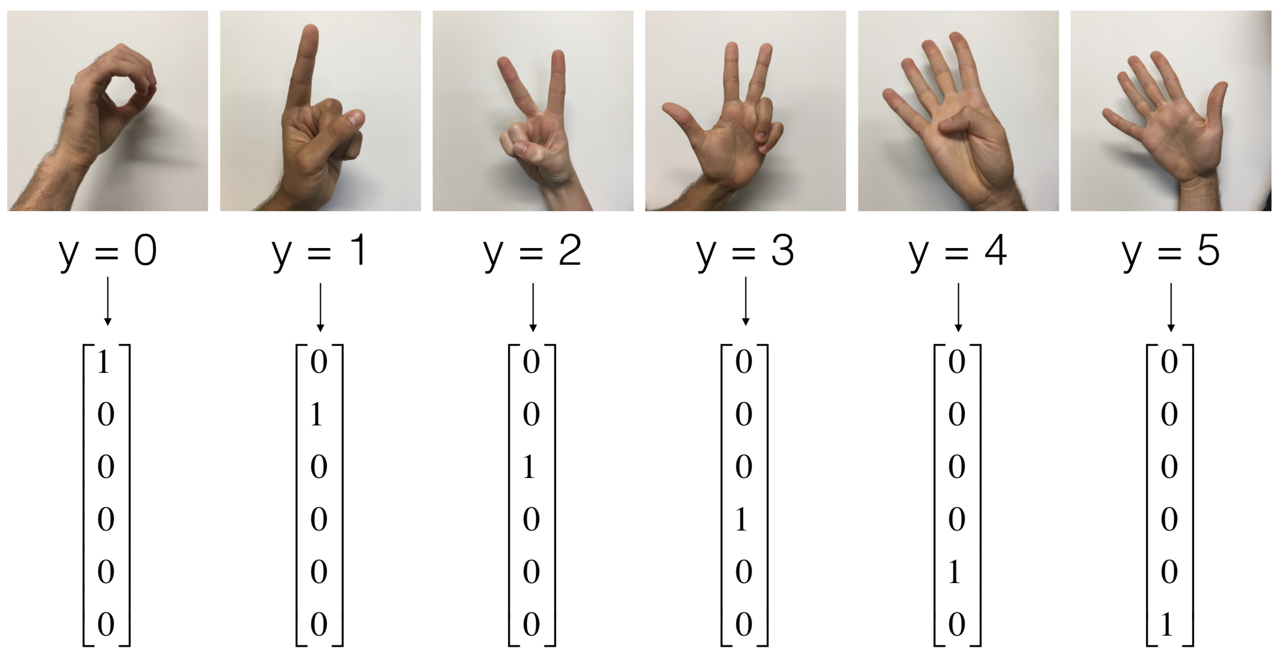
Sign Language Detection**
- Task: Given an image of a hand showing a number (0–5) in sign language, predict the number.
-
Application: Sign translation systems and assistive technologies for people with hearing or speech impairments.
- The figure below shows a network trained to classify hand gestures into digits. Each hand image is processed into pixels, which are fed through convolutional or fully connected layers. The learned filters capture distinctive finger arrangements, allowing accurate classification.
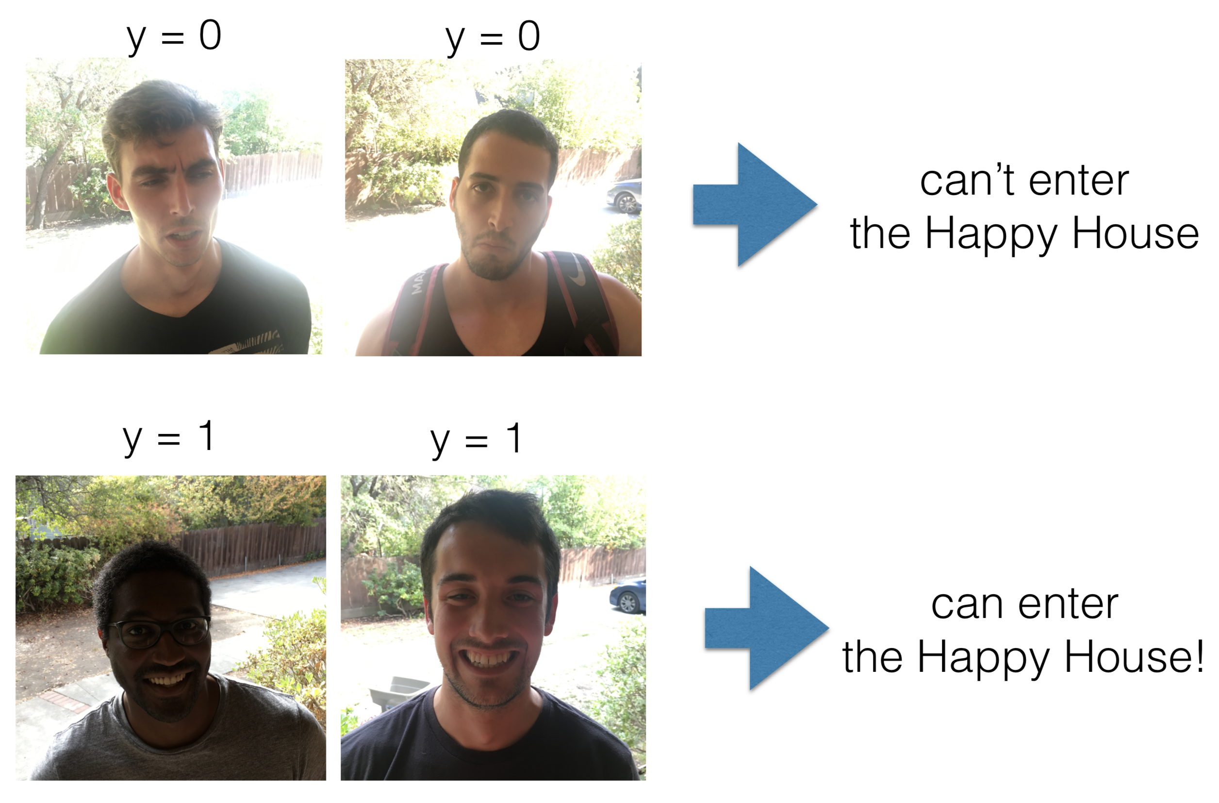
The Happy House (Sentiment-based Filtering)**
- Task: A playful application where only smiling people are let inside.
-
Application: Demonstrates sentiment analysis from images, analogous to how models classify emotion in faces or tone in voice.
- The following figure shows how the system evaluates face images, classifies whether the person is smiling, and decides whether to “let them in.” While playful, it reflects the same technical principles used in real-world sentiment or affect detection.
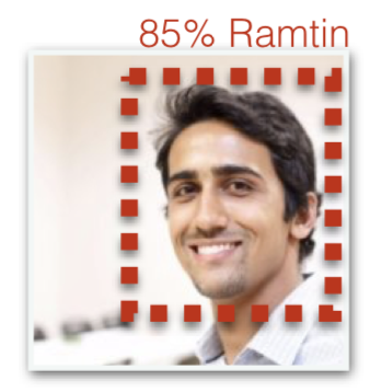
Face Recognition**
- Task: Given an image of a person, predict their identity.
-
Application: Authentication (phone unlocks), surveillance, and photo tagging.
- In the figure below, a face image is transformed into an embedding vector that encodes identity-specific features such as eye spacing or jaw shape. Recognition is performed by comparing embeddings across a database. This application relies heavily on convolutional neural networks for feature extraction.
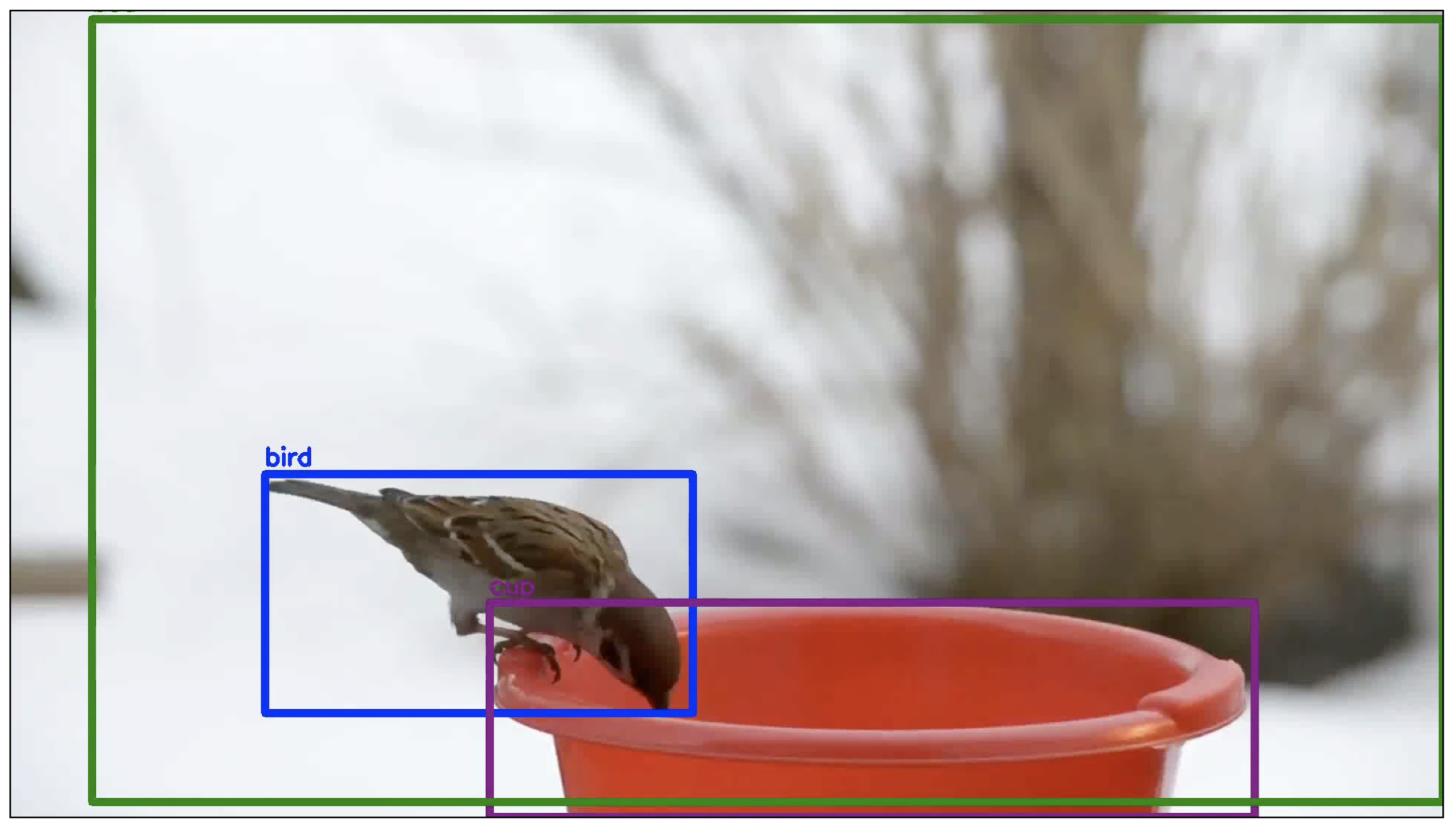
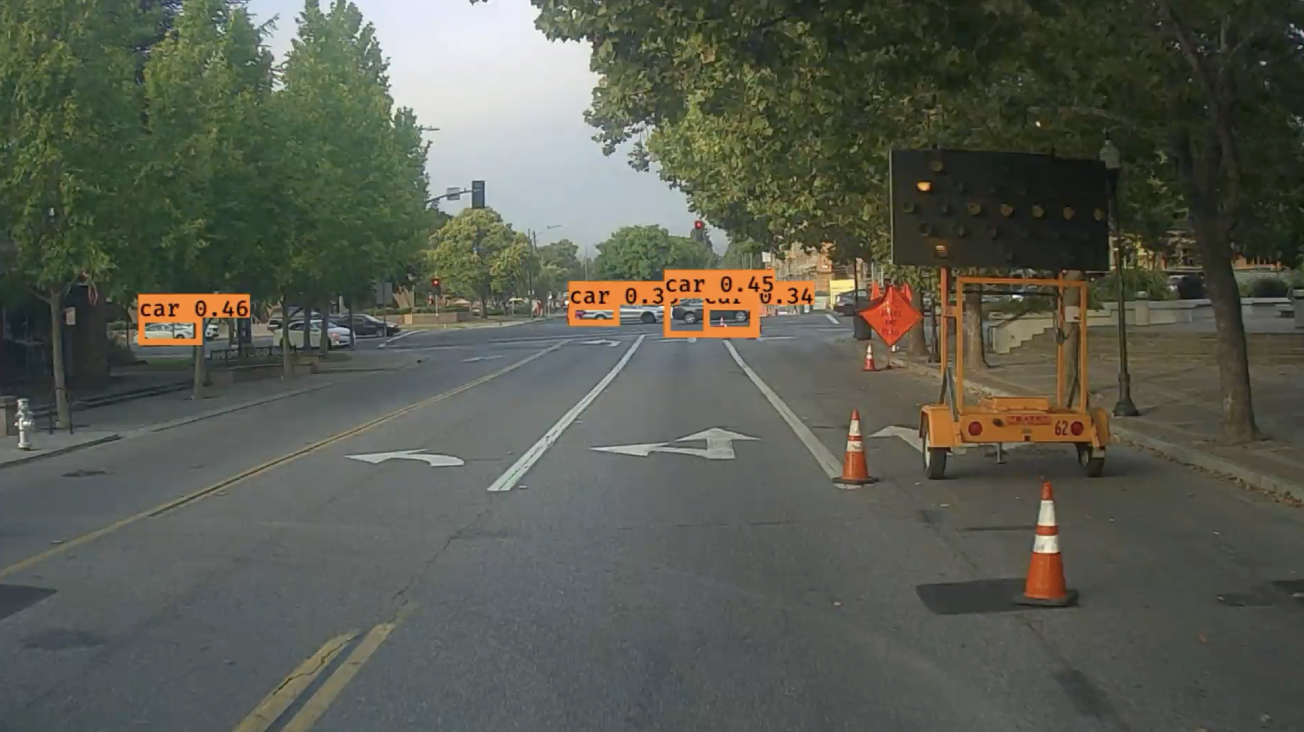
Object Detection for Autonomous Driving**
- Task: Detect and classify objects such as pedestrians, traffic signs, and vehicles in real time.
-
Application: Perception systems in self-driving cars.
- The figure below demonstrates a neural network (e.g., YOLO or Faster R-CNN) identifying multiple objects in a scene. Bounding boxes localize objects, and class labels (e.g., “car,” “pedestrian”) are predicted simultaneously.
- A complementary figure highlights car detection specifically, a key element of self-driving pipelines.
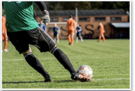
Sports Analytics: Goalkeeper Shoot Prediction**
- Task: Predict the optimal region where a soccer player should shoot the ball to maximize scoring chances.
-
Application: Sports strategy, player training, and performance analytics.
- The figure illustrates how a neural network predicts probability maps over the goal area. Bright regions indicate higher scoring potential, guiding players on where to shoot.
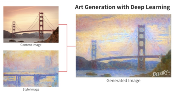
Art Generation (Neural Style Transfer)**
- Task: Merge the content of one image with the artistic style of another.
-
Application: Creative AI in digital art, media, and design.
- The figure demonstrates how CNNs can extract style statistics (colors, textures) from one image and content structure from another, producing a new composite artwork.
Music Generation**
- Task: Train a sequence model to generate music.
-
Application: Algorithmic composition, soundtrack generation, and creative tools.
- The following figure depicts how recurrent or sequence models learn temporal dependencies in audio data, enabling them to generate plausible melodies.

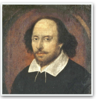
Text Generation**
- Task: Generate new text in the style of a given corpus (e.g., Shakespeare).
-
Application: Creative writing assistants, dialogue systems, chatbots.
- The figure illustrates a sequence model trained on Shakespeare’s works generating stylistically consistent lines of verse.
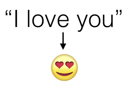
Sentiment Analysis and Emoji Prediction**
- Task: Map input sentences to emojis that capture their sentiment.
-
Application: Messaging apps, predictive emoji keyboards, smart suggestions.
- The figure shows a neural model classifying text sentiment and mapping it to emojis. This demonstrates how embeddings capture semantic meaning of sentences.
Machine Translation**
- Task: Translate text between languages.
-
Application: Breaking language barriers in communication, international collaboration, and commerce.
- The following figure highlights neural machine translation, where a sequence-to-sequence model encodes a source sentence and decodes it into a target language.

Trigger Word Detection**
- Task: Detect when a specific word or phrase is spoken (e.g., “Hey Siri,” “OK Google”).
-
Application: Voice assistants and smart speakers.
- The figure shows a speech signal fed into a neural network that continuously monitors for the trigger word. Once detected, the system activates additional features such as query processing.

Architectures of Neural Networks
-
Neural networks are not restricted to a single design; instead, they can be configured in many different architectures depending on the problem. The choice of architecture determines how the network processes information, the kinds of dependencies it can model, and its effectiveness for specific data types such as images, text, or sequential signals.
-
Fully connected layers (dense networks) are the most basic form, where every neuron in one layer connects to every neuron in the next. While powerful for structured data like real estate or advertisement click prediction, these architectures struggle with high-dimensional unstructured data such as images or speech, where local patterns and sequential dependencies matter.
-
For these cases, specialized architectures emerge:
- Convolutional Neural Networks (CNNs) for spatially structured data like images and video.
- Recurrent Neural Networks (RNNs) and their modern variants (e.g., LSTMs, GRUs, Transformers) for sequential data like language, speech, or time series.
- Hybrid architectures for complex tasks like autonomous driving, which require combining vision, control, and temporal reasoning.
-
The following figure illustrates these basic network families side by side: fully connected feedforward networks, CNNs with local receptive fields, and RNNs with recurrent feedback loops. It also highlights how hybrid designs can be assembled to handle multimodal problems.

-
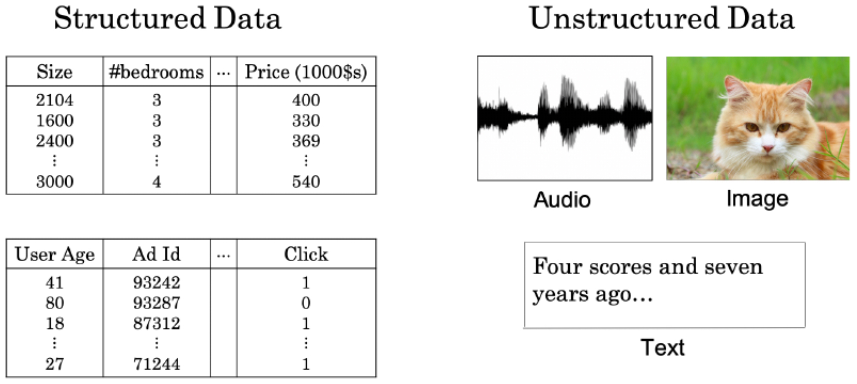
Another important axis of distinction is whether networks operate on structured data (tables, databases, numerical features) or unstructured data (images, audio, free text). Traditional machine learning was successful on structured data because feature engineering could encode domain knowledge. By contrast, unstructured data resisted these approaches, requiring handcrafted features like SIFT for images or MFCCs for audio.
-
Deep learning revolutionized this space by learning representations directly from raw inputs. CNNs automatically learn edge detectors, textures, and object parts. RNNs and Transformers learn long-range dependencies in text and speech. This has enabled machines to rival or even surpass human performance in tasks that were once considered uniquely human.
-
The following figure contrasts these domains: structured data, where classical ML excels, versus unstructured data, where deep learning has been transformative.
-
In summary, neural network architectures are designed with inductive biases that match the structure of the data:
- Spatial locality \(\rightarrow\) Convolutions (CNNs).
- Temporal or sequential order \(\rightarrow\) Recurrence and attention (RNNs, Transformers).
- Mixed modalities \(\rightarrow\) Hybrid models.
-
This modularity explains why deep learning is such a general-purpose paradigm: by choosing the right architecture, we can adapt the same underlying principles to almost any type of data.
Logistic Regression as a Neural Network
-
Logistic regression is often introduced as a simple classification algorithm, but it can also be viewed as the simplest neural network. In this perspective, logistic regression is a one-layer network with no hidden layers: it takes an input vector, applies a linear transformation, and passes the result through a nonlinear activation function (the sigmoid). While limited in expressive power, this model lays the foundation for understanding more complex deep learning architectures.
-
By grounding the mathematics of logistic regression in both theory and practical applications, we see how this “baby neural network” connects to the much larger, multi-layer systems used in modern AI.
Notation
-
Each dataset consists of training and test examples. Let
- \(m_{\text{train}}\) = number of training examples
- \(m_{\text{test}}\) = number of test examples
-
Each training example is a pair:
\[(x^{(i)}, y^{(i)}), \quad x^{(i)} \in \mathbb{R}^{n_x}, \quad y^{(i)} \in \{0,1\}\]- where, \(x^{(i)}\) is the input feature vector, and \(y^{(i)}\) is the binary label (yes/no, cat/non-cat, spam/non-spam, etc.).
-
We collect all inputs into a data matrix:
- … and all outputs into a label vector:
- This compact matrix notation allows us to leverage vectorized operations, which are crucial for scaling to large datasets.
Binary Classification
-
A binary classifier predicts whether an input belongs to one of two classes, labeled 1 (positive) or 0 (negative). For example, given an image, we may want to classify it as containing a cat (1) or not containing a cat (0).
-
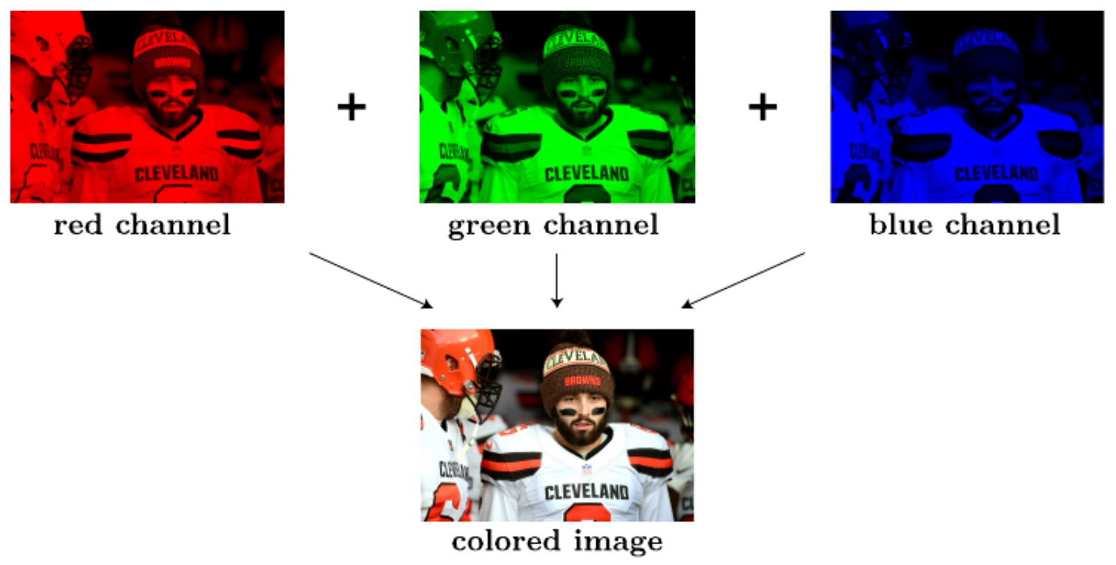
Images are typically stored as arrays of pixel values. For color images, each pixel has three intensity values corresponding to the red, green, and blue channels. The following figure illustrates this representation:
- To use such an image in logistic regression, we flatten the pixel values into a long column vector. For an image of size \(n \times m\), with 3 channels (RGB), the feature vector is of length:
-
Thus, each example \(x^{(i)}\) becomes a high-dimensional input vector. Even small images (e.g., 64 × 64 pixels) yield thousands of input features.
-
This setup bridges traditional machine learning with modern deep learning: logistic regression shows us how a simple linear model can classify data, but it also highlights the need for more expressive models when the feature space becomes very high-dimensional or when input patterns are complex.
Logistic Regression Cost Function
-
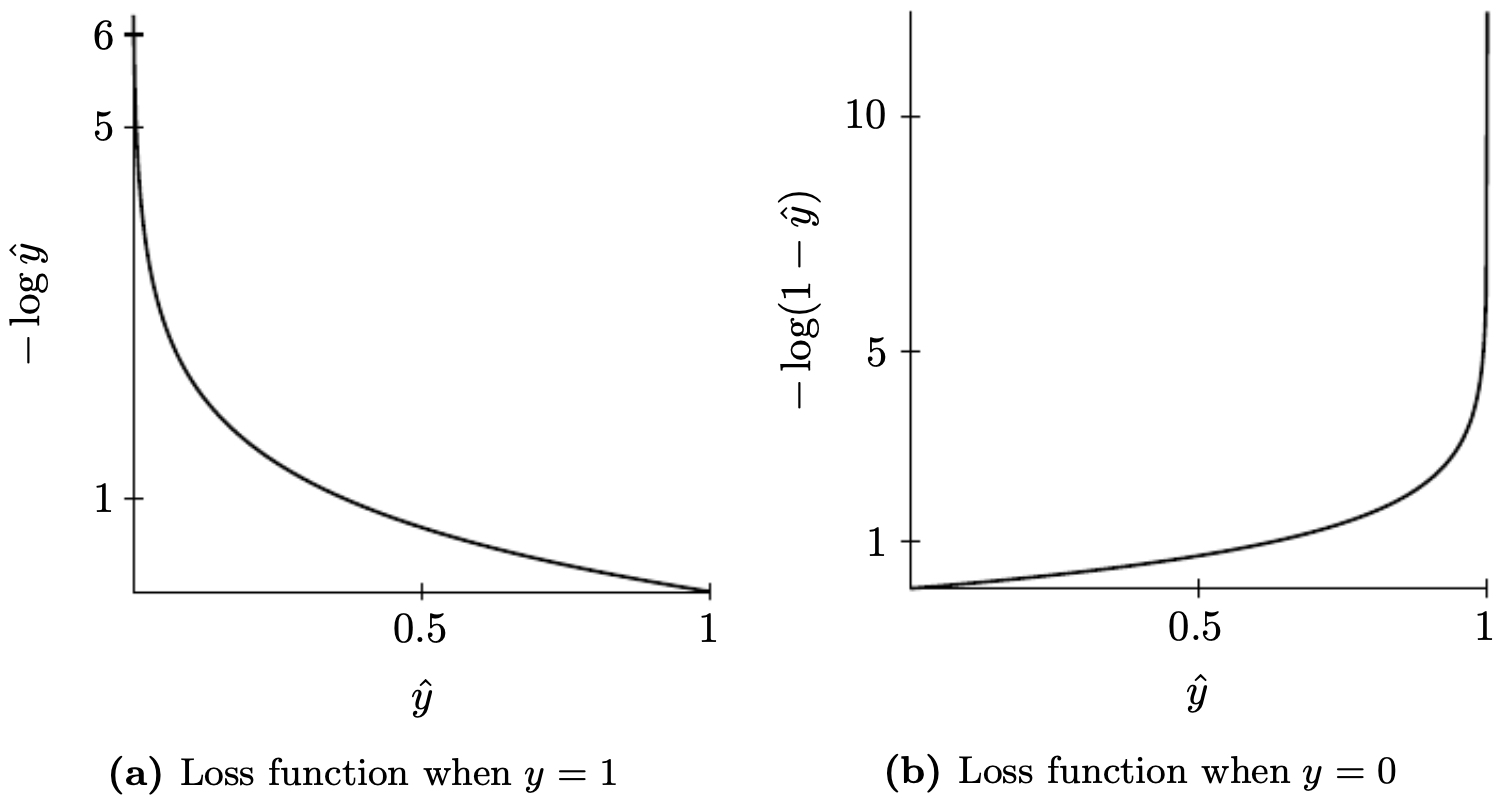
To train logistic regression, we need a cost function that measures how well our model’s predictions \(\hat{y}\) match the true labels \(y\). The standard choice is the logistic loss (also called cross-entropy loss):
\[L(\hat{y}, y) = - \Big[ y \log(\hat{y}) + (1-y)\log(1-\hat{y}) \Big]\]- If the true label is \(y=1\), the loss reduces to \(- \log(\hat{y})\), which penalizes the model heavily when \(\hat{y}\) is small.
- If the true label is \(y=0\), the loss reduces to \(- \log(1-\hat{y})\), which penalizes predictions close to 1.
-
The overall cost function across all \(m\) training examples is the average logistic loss:
-
This function is convex, meaning it has a single global minimum and no local minima. This property guarantees that optimization algorithms like gradient descent can find the best parameters \(w\) and \(b\) efficiently.
-
The following figure visualizes the binary classifier’s loss behavior for the two cases (when \(y=1\) and when \(y=0\)). Notice how the loss skyrockets if the model makes confident but incorrect predictions, forcing the model to adjust weights toward better classification.
- This cost function forms the backbone of logistic regression and serves as the simplest example of using probability theory to derive principled learning objectives.
Gradient Descent
-
Once we have defined the logistic regression cost function, the next step is to minimize it in order to find the best parameters \(w\) and \(b\). The most widely used optimization algorithm for this is gradient descent.
-
The update rules are:
\[w := w - \alpha \frac{\partial J}{\partial w}, \qquad b := b - \alpha \frac{\partial J}{\partial b}\]- where:
- \(\alpha\) is the learning rate (a small positive number controlling step size),
- \(\frac{\partial J}{\partial w}\) and \(\frac{\partial J}{\partial b}\) are the gradients of the cost function with respect to the model parameters.
- where:
Deriving the Gradients
- For logistic regression:
- … the gradients turn out to be:
-
This means:
- The weight gradient for feature \(j\) is the average difference between predictions and labels, weighted by that feature’s value.
- The bias gradient is just the average prediction error across all training examples.
Optimization Landscape
-
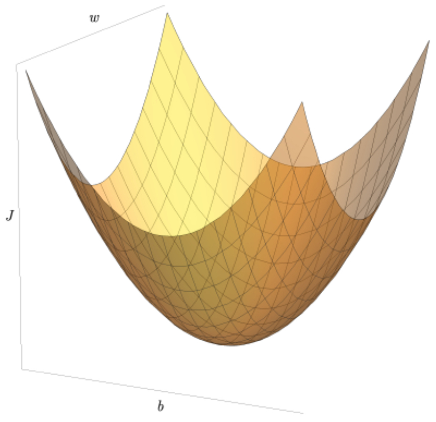
Because the logistic regression cost function is convex, gradient descent will converge to the global minimum as long as the learning rate is chosen appropriately (not too large, not too small).
-
The following figure illustrates a convex cost surface where gradient descent gradually descends toward the global minimum, step by step.
- With gradient descent, logistic regression learns parameters that minimize classification errors over the dataset. This simple yet powerful procedure is also the foundation of optimization in deep learning, where the same principle is applied to far more complex neural networks.
Computation Graphs and Backpropagation
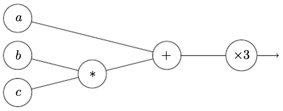
- To better understand how gradient descent works in practice, it is useful to represent computations as a computation graph. A computation graph explicitly shows the sequence of operations required to compute the final output, making it easier to organize both the forward pass (calculating the output) and the backward pass (computing gradients using the chain rule).
Example: Simple Computation
- Suppose we want to compute:
-
The computation can be broken down into smaller steps:
- Compute the product: \(u = b \cdot c\)
- Add to \(a\): \(v = a + u\)
- Multiply by 3: \(J = 3v\)
-
This sequence is represented in the following figure as a computation graph, where each node corresponds to an operation and edges carry values forward.
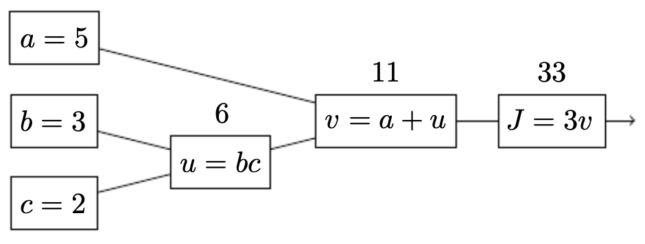
Forward Pass
-
In the forward pass, we move from inputs to the output:
- Multiply \(b\) and \(c\) to get \(u\).
- Add \(a\) and \(u\) to get \(v\).
- Multiply \(v\) by 3 to get \(J\).
-
The computation graph makes these steps explicit, showing intermediate variables and dependencies.
-
The next figure illustrates the same computation but now highlights the intermediate variables \(u\), \(v\), and \(J\) in the graph.
Backward Pass: Applying the Chain Rule
-
The real power of computation graphs lies in how they simplify gradient computation. Using the chain rule, we can systematically compute derivatives step by step in reverse (backpropagation).
-
From the output:
- \[\frac{\partial J}{\partial v} = 3\]
- \[\frac{\partial v}{\partial a} = 1, \quad \frac{\partial v}{\partial u} = 1\]
- \[\frac{\partial u}{\partial b} = c, \quad \frac{\partial u}{\partial c} = b\]
-
Thus the gradients are:
\[\frac{\partial J}{\partial a} = \frac{\partial J}{\partial v} \cdot \frac{\partial v}{\partial a} = 3\] \[\frac{\partial J}{\partial b} = \frac{\partial J}{\partial v} \cdot \frac{\partial v}{\partial u} \cdot \frac{\partial u}{\partial b} = 3c\] \[\frac{\partial J}{\partial c} = \frac{\partial J}{\partial v} \cdot \frac{\partial v}{\partial u} \cdot \frac{\partial u}{\partial c} = 3b\]
Why This Matters
- In logistic regression, and more generally in deep learning, every cost function is ultimately built from a chain of simpler computations (linear combinations, activations, multiplications, additions).
- Backpropagation allows us to efficiently compute gradients for all parameters by systematically applying the chain rule on the computation graph.
- This approach scales seamlessly from simple models to deep networks with millions of parameters.
From Logistic Regression to Student Projects
- While logistic regression may appear simple, it lays the conceptual foundation for more advanced neural network models. The ideas of mapping inputs to outputs, optimizing parameters with gradient descent, and computing gradients via backpropagation extend naturally into deep learning. In fact, many real-world applications can be viewed as sophisticated extensions of logistic regression.
Coloring Black & White Pictures with Deep Learning
-
One fascinating application is automatic photo colorization. Here, the input is a grayscale image (single channel), and the task is to predict the missing color channels (RGB). Conceptually, this is just a regression problem applied at the pixel level: the model predicts a distribution of possible RGB values for each grayscale input pixel.
-
The following figure shows an example project where deep learning models bring black-and-white photos to life by predicting realistic colors. The model essentially learns semantic associations — for instance, skies tend to be blue, grass tends to be green, and skin tones follow natural distributions.

Predicting the Price of an Object from a Picture
-
Another project combines regression with interpretability: predicting the price of an object, such as a bike, directly from its image. The neural network not only maps pixels to a price but also learns to focus attention on visually discriminative features, such as the presence of extra wheels in kids’ bikes or advanced suspension systems in racing bikes.
-
The figure below illustrates this task, where the model highlights relevant regions in the image that strongly influence its price prediction.
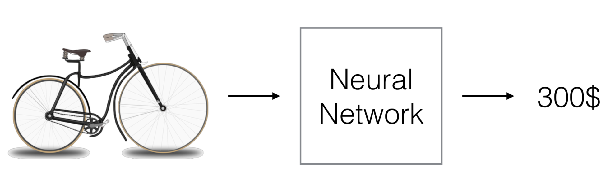
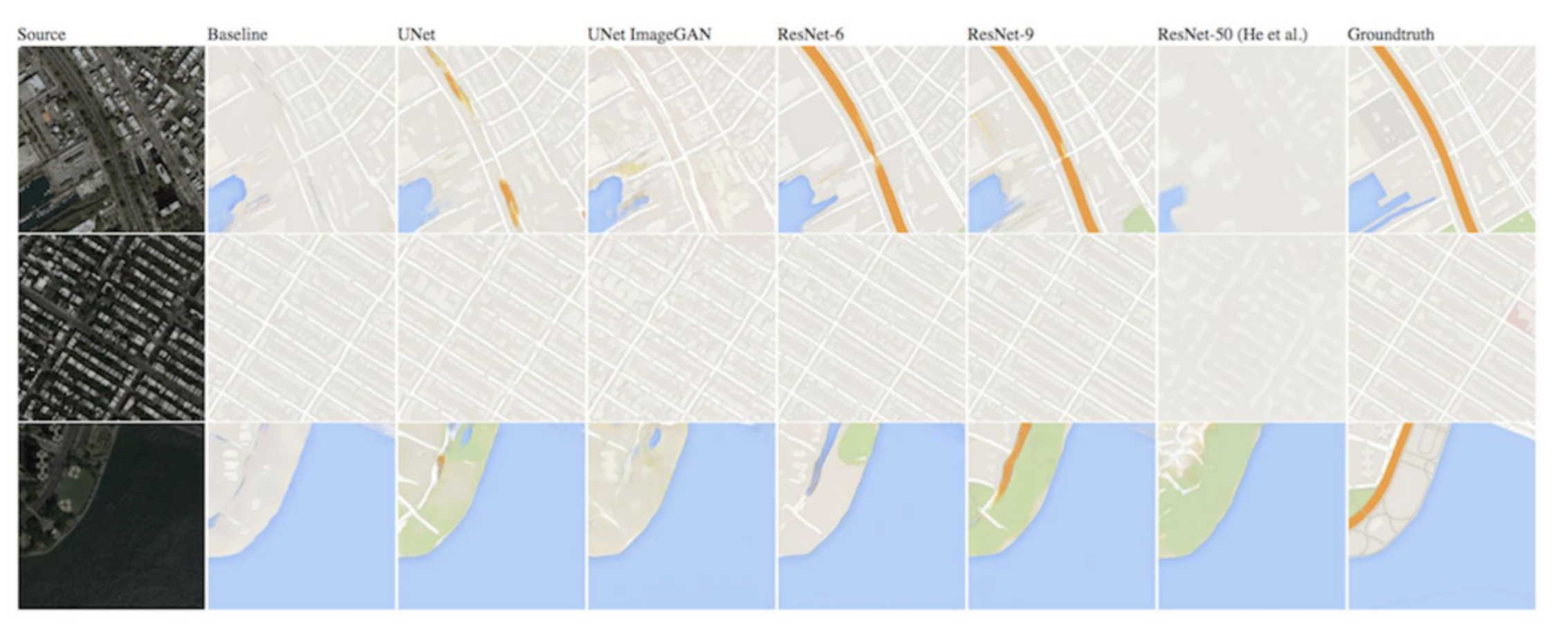
Image-to-Image Translation with Conditional GANs
-
In more advanced settings, models like conditional GANs (Generative Adversarial Networks) extend the principles of logistic regression into adversarial learning. For example, given a satellite image, the model can generate a corresponding map. One network (the generator) produces candidate outputs, while another (the discriminator, akin to logistic regression) classifies whether the generated image is real or fake.
-
The figure below shows this process, where satellite imagery is translated into map-like renderings using architectures such as U-Net and ResNet.
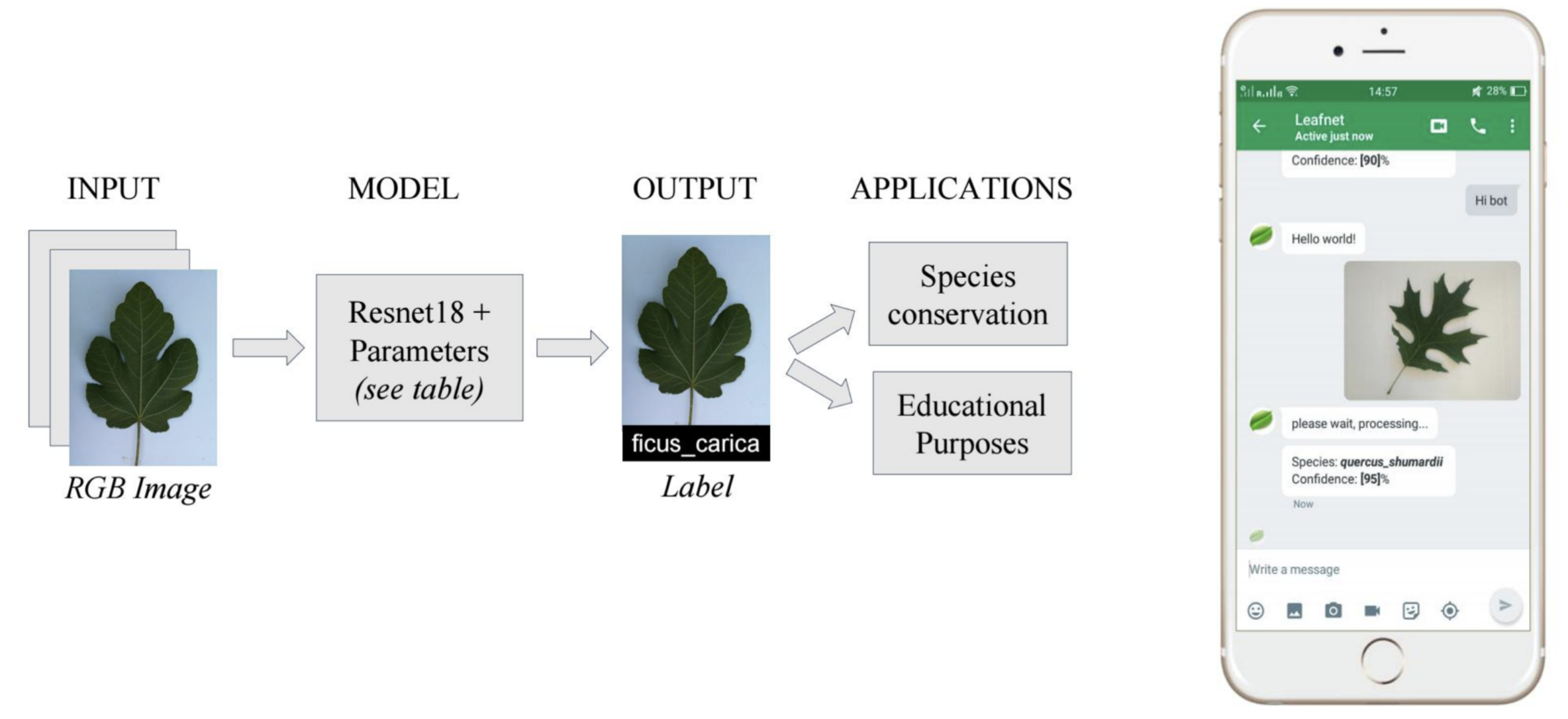
LeafNet: Tree Species Identification
-
Finally, a classic supervised learning task is multiclass classification, which generalizes logistic regression beyond binary labels. For instance, LeafNet predicts tree species based on photographs of leaves. Each image is passed through a deep neural network that outputs probabilities across many possible species, and the model selects the species with the highest probability.
-
The following figure shows LeafNet in action, a project where students trained a model to classify tree species using only leaf photographs.
Takeaway
-
These projects highlight the journey from logistic regression to modern applications:
- Photo colorization \(\rightarrow\) regression at the pixel level.
- Price prediction from images \(\rightarrow\) regression with feature interpretability.
- Image-to-image translation \(\rightarrow\) adversarial classification built on logistic regression principles.
- Tree species classification \(\rightarrow\) extension from binary to multiclass logistic regression.
-
At their core, these diverse applications are all powered by the same principles: representing inputs numerically, computing predictions, defining a cost function, and minimizing it with gradient-based optimization.
Python and Vectorization
- One of the main bottlenecks in deep learning is not just designing neural networks, but scaling them to massive datasets. Applications like machine translation, speech recognition, and high-resolution image generation often require millions (or even billions) of examples. Training on such data with naive, loop-based code would take unreasonably long. This is where vectorization becomes essential. By removing explicit loops and relying on fast, optimized linear algebra libraries (like NumPy or BLAS) that exploit parallelism on CPUs and GPUs, we can reduce weeks of computation to hours.
Vectorization
-
The goal of vectorization is to eliminate slow Python loops by rewriting computations in terms of efficient matrix and vector operations. For example, in logistic regression we often compute
\[z = w^T x + b\]- where \(w \in \mathbb{R}^{n_x}\) and \(x \in \mathbb{R}^{n_x}\).
-
A naive implementation might loop over each feature:
z = 0
for j in range(nx):
    z += w[j] * x[j]
z += b
- This approach is O(n_x) in Python and scales poorly. Instead, NumPy provides optimized functions that run in C under the hood:
z = np.dot(w, x) + b
- This one-liner eliminates the loop and leverages optimized libraries that can run across multiple cores or GPUs.
Vectorizing Logistic Regression
- For a dataset with many training examples, looping is even worse. For each example \(x^{(i)}\), we compute
- Stacking all inputs into a matrix:
-
… we can write the vectorized form as:
\[Z = w^T X + b, \quad A = \sigma(Z),\]- where \(\sigma\) is applied elementwise.
-
In NumPy:
Z = np.dot(w.T, X) + b
A = 1 / (1 + np.exp(-Z))
- This replaces an explicit \(O(m \cdot n_x)\) loop with a single matrix multiplication that runs in optimized C code.
Vectorizing Gradient Computation
- The cost function gradients for logistic regression are
- Vectorized implementation in NumPy:
dZ = A - Y
dw = np.dot(X, dZ.T) / m
db = np.sum(dZ) / m
- Instead of looping over \(m\) training examples, we compute everything with just a few matrix multiplications and reductions.
Broadcasting
-
Vectorization is often paired with broadcasting, where NumPy automatically expands arrays to match dimensions. This avoids unnecessary replication of data.
-
Suppose we want to normalize each column of a matrix \(A \in \mathbb{R}^{3 \times 4}\) by the column sums:
-
In NumPy:
s = np.sum(A, axis=0).reshape(1,4) A_normalized = A / s- where,
shas shape(1,4), but NumPy broadcasts it across the 3 rows ofA.
- where,
-
Other examples of broadcasting:
- Scalar broadcast:
- Row vector broadcast:
- Column vector broadcast:
A Note on NumPy Vectors
- A subtle but important detail:
a = np.random.randn(5)
print(a.shape)  # (5,)
- This is a rank-1 array. It is neither a row vector nor a column vector, and
a.Thas no effect. For clarity, in deep learning it’s preferable to explicitly use column vectors:
a = np.random.randn(5,1) # shape (5,1)
- This ensures dot products and broadcasting behave as expected.
Why Vectorization Matters in Practice
-
Without vectorization, modern neural networks would not be practical.
- Student projects like LeafNet or Satellite Map Translation involve thousands of high-resolution images. Vectorization allows training in hours instead of weeks.
- Industrial-scale tasks like machine translation or speech recognition require processing billions of tokens or hours of audio. Vectorization (plus GPU/TPU acceleration) makes this possible.
-
Deep architectures — from CNNs to Transformers — are ultimately built from the same linear algebra operations: matrix multiplications and tensor contractions.
- Thus, vectorization is not just a coding convenience — it is the cornerstone of modern deep learning scalability.
Citation
If you found our work useful, please cite it as:
@article{Chadha2020IntroToDeepLearning,
  title   = {Introduction to Deep Learning},
  author  = {Chadha, Aman},
  journal = {Distilled Notes for Stanford CS230: Deep Learning},
  year    = {2020},
  note    = {\url{https://aman.ai}}
}