CS230 • Interpretability of Neural Networks
- Introduction
- Interpreting the Neural Networks’ Outputs
- Visualizing Neural Networks from the Inside
- The Deconvolution and Its Applications
- Takeaways
- Citation
Introduction
-
Deep neural networks (DNNs), particularly convolutional neural networks (CNNs), have achieved remarkable success in image classification, detection, and segmentation tasks. Despite their empirical effectiveness, these models are often perceived as “black boxes,” where the internal decision-making processes remain opaque. This lack of interpretability is a central barrier to the adoption of deep learning models in high-stakes domains such as healthcare, law, and autonomous systems.
-
In this primer, we focus on interpreting the outputs of trained neural networks and visualizing their inner workings. Specifically, we introduce tools such as saliency maps, occlusion sensitivity analysis, and localization methods, before moving into deeper visualization techniques such as gradient ascent and dataset search. We conclude with the discussion of deconvolution and unpooling as ways of reconstructing input data from intermediate activations.
-
The following figure (source) illustrates the motivation for this study: the need to transform opaque decision-making into transparent visualizations that can be scrutinized by humans. It depicts the challenge of interpreting CNN decisions, where the model has high predictive accuracy but limited transparency in its reasoning process.
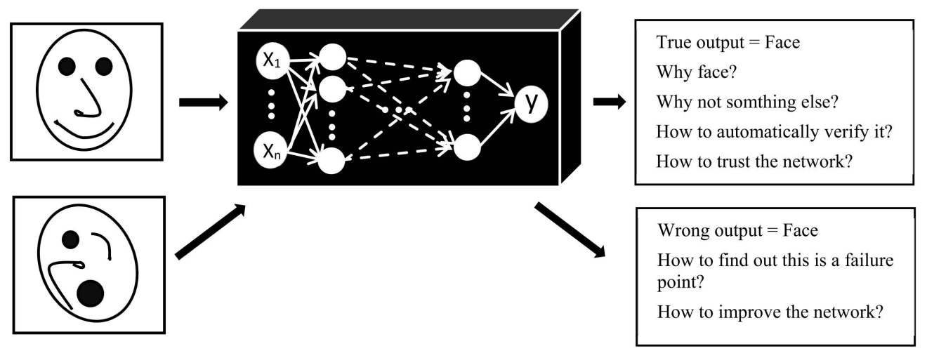
- With these interpretability tools, we aim not only to improve trust in neural networks but also to gain insights into how they encode features, represent knowledge, and prioritize regions of input data. By unpacking the decision mechanisms of CNNs, we build a bridge between algorithmic efficiency and human understanding.
Interpreting the Neural Networks’ Outputs
-
One of the major challenges in applying CNNs to real-world problems is not only verifying their accuracy but also demonstrating that their decisions are grounded in meaningful input features. For example, suppose we train a CNN for animal classification in a pet shop scenario. While the model achieves high predictive accuracy, the manager may remain skeptical:
- Is the CNN really identifying the animal?
- Or is it exploiting spurious correlations, such as background color or shadows?
-
To address these concerns, we turn to interpretability methods. These approaches provide visualizations that reveal which parts of the input image most influence the model’s decision.
Building Saliency Maps through Derivative Analysis
-
A foundational technique for interpreting CNN predictions is the saliency map, which leverages gradient information. Consider the score assigned to the “dog” class before the softmax activation:
- Let the score be denoted by \(s_{\text{dog}}(x)\).
- The saliency map is computed as the gradient of this score with respect to the input image \(x\):
-
This gradient identifies the pixels that need to change the least in order to produce the largest impact on the class score. In essence, it highlights the sensitive regions of the input image that drive the decision.
-
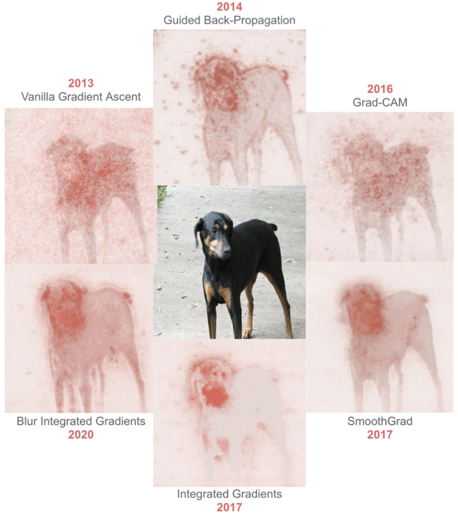
The following figure (source) demonstrates how a saliency map highlights the regions of an image most critical to a CNN’s classification decision. Notice how the pixels corresponding to the animal itself, particularly the edges and distinctive features (e.g., ears, eyes, and paws), have high gradients, while the background pixels show little influence.
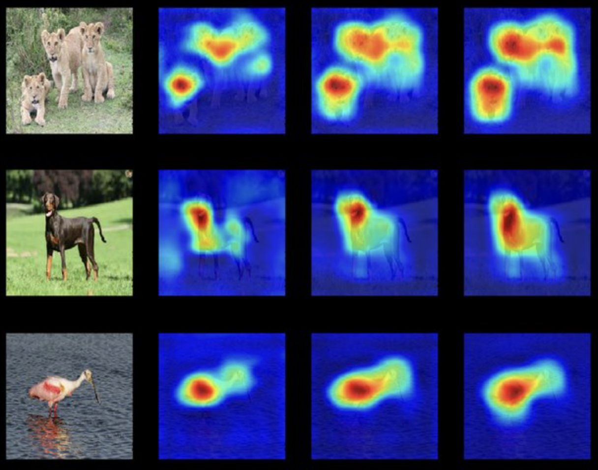
- Saliency maps can further be used for image segmentation tasks, as they provide a soft attention mask over relevant pixels.
Building Probability Maps via Analyzing Occlusion Sensitivity
-
While saliency maps rely on derivatives, occlusion sensitivity analysis takes a perturbation-based approach. The idea is simple:
- Block (occlude) a rectangular patch in the input image.
- Measure the effect of the occlusion on the CNN’s output score.
- Repeat this process by sliding the patch across the entire image.
-
Formally, let \(x\) denote the input image, and \(x_{(i,j)}^{\text{occluded}}\) denote the image with a patch occluding region \((i,j)\). The new score is:
-
Comparing \(s_{\text{dog}}^{(i,j)}\) with the original score \(s_{\text{dog}}(x)\) reveals how important region \((i,j)\) was for the classification. Aggregating these differences across all patches yields a probability map.
-
The following figure shows the result of an occlusion sensitivity analysis. If the occlusion is not in a central part of the image, the class probability does not drop significantly. Conversely, the CNN’s confidence drops sharply when the occlusion overlaps with the animal, producing a high-impact region on the map.
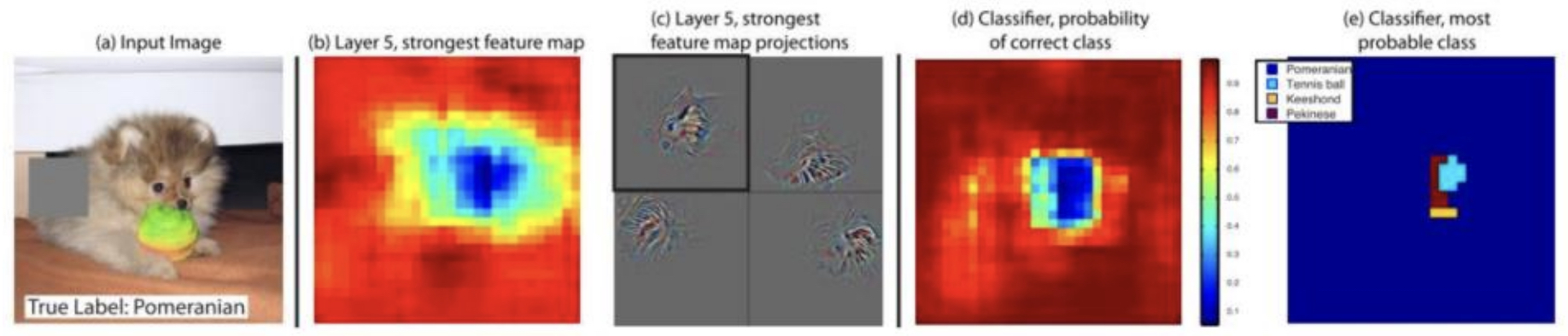
- This method is particularly useful for validating whether the CNN is truly focusing on the animal or mistakenly relying on irrelevant cues like the cage, floor, or background texture.
Interpreting Neural Networks for Object Localization
-
Beyond classification, many practical applications require localization: identifying where in the image the object resides. Interestingly, a trained CNN classifier can often be adapted into a localizer with only minor modifications.
-
In a standard CNN classifier:
- The final convolutional feature maps are flattened into a vector.
- This vector is passed into fully connected (dense) layers.
- Location information is effectively discarded at the flattening stage.
-
To preserve spatial information, we can replace flattening with global average pooling (GAP). GAP computes the mean activation across each feature map, directly connecting spatial patterns to class predictions.
-
Formally, for a feature map \(A^k\) at the final convolutional layer, the GAP operation is:
\[z^k = \frac{1}{Z} \sum_{i} \sum_{j} A^k_{i,j}\]- where \(Z\) is the number of spatial positions. The pooled outputs \(\{z^k\}\) are then fed into the final classification layer with learned weights \(w_k^c\). The resulting class activation map (CAM) for class \(c\) is:
-
This heatmap directly localizes the discriminative regions for class \(c\).
-
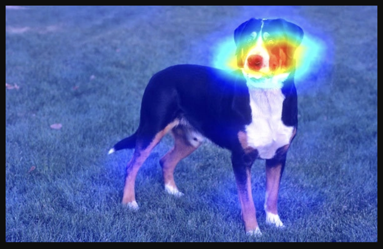
The following figure (source) shows how class activation maps (CAMs) transform a classifier CNN into a localizer, where the CNN highlights the precise location of the dog contributing to its classification.
-
This simple architectural adjustment allows the same CNN to serve both classification and localization purposes, bridging the gap between prediction accuracy and interpretability.
Visualizing Neural Networks from the Inside
-
While saliency maps and occlusion sensitivity help us interpret which parts of the input are important for predictions, they do not fully reveal what the network has learned internally. To gain deeper insights, we can explore how the network “thinks” about objects by directly visualizing activations and optimizing inputs to probe its representations.
-
Two complementary approaches are particularly effective:
- Gradient ascent optimization to synthesize representative inputs.
- Dataset search to find real examples that maximally activate certain neurons.
-
Together, these approaches provide both synthetic and empirical perspectives on the learned features of a CNN.
Gradient Ascent Optimizer for Visualizing Neural Networks
- The intuition behind this approach is straightforward: if we want to know how the network internally represents “dog,” we can construct an input image that maximizes the dog-class score. This is done by applying gradient ascent on the input space.
Method
- Given a class score \(s_{\text{dog}}(x)\), we define the optimization objective as:
-
Here, the second term acts as a regularization penalty to ensure that the synthesized image remains natural-looking rather than turning into noisy artifacts.
-
The gradient ascent procedure iterates as follows:
- Forward propagate the current input \(x\).
- Compute the loss \(L(x)\).
- Backpropagate to obtain \(\frac{\partial L}{\partial x}\).
- Update the image pixels with a small step in the gradient direction:
-
After several iterations, \(x\) evolves into a pattern that strongly excites the “dog” neuron.
-
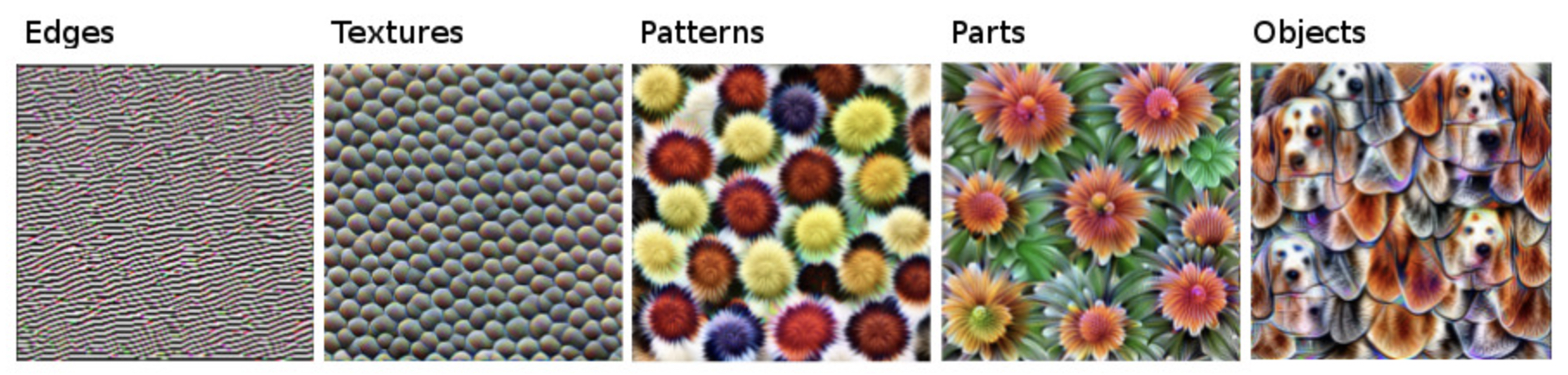
The following figure (source) demonstrates this process, where an initially random input image is iteratively updated through gradient ascent-based techniques to resemble a prototypical dog-like pattern. Put simply, it shows how gradient ascent transforms noise into a recognizable representation of a dog by maximizing the class score.
- This technique is not limited to class scores. It can also be applied to intermediate activations within the network. For instance, maximizing the activation of neuron \(a^l_j\) in layer \(l\) yields insight into what that neuron responds to—edges, textures, or object parts.
Dataset Search for Visualizing Neural Networks
- While gradient ascent produces synthetic prototypes, another strategy is to search the training dataset for real images that maximally activate a neuron or feature map. This method helps ground our interpretations in actual data.
Method
- For a neuron activation \(a^l_j(x)\), we compute activation scores across the dataset:
-
Then, we rank all inputs by this score and retrieve the top \(k\) images (e.g., \(k = 5\)).
-
This reveals which types of patterns or objects most excite the neuron in practice. For example, a neuron in a convolutional layer may consistently activate for vertical stripes, or another may light up for human faces.
-
The following figure (source) illustrates this dataset search technique, where the top-5 most activating images for a neuron all contain shirts with similar textures and colors.
Complementary Insights
- Gradient ascent exposes the idealized concept that excites a neuron, free from dataset biases.
-
Dataset search grounds this concept in real-world samples, revealing how the neuron behaves in practice.
- By combining these techniques, we obtain a clearer picture of both the abstract features learned by CNNs and their manifestations in real data. This dual perspective strengthens our interpretability toolkit.
The Deconvolution and Its Applications
-
Convolutional neural networks are fundamentally built on the convolution operation, which compresses spatial information into increasingly abstract representations. However, in some cases, we want to invert this process: given an activation inside the network, can we reconstruct the original input pattern that caused it?
-
This is the motivation behind deconvolution (also called transposed convolution). Deconvolution techniques are central to applications such as generative models (e.g., GANs) and semantic segmentation, where networks must produce detailed images or pixel-level masks rather than just high-level labels.
Introduction
-
Conceptually, deconvolution can be understood in two complementary ways:
- As a transpose of the convolution operation, where the flow of information is reversed.
- As an approximate inversion of convolution, allowing us to map feature activations back into input space.
-
This process enables visualization of what activations correspond to, as well as practical reconstruction tasks.
-
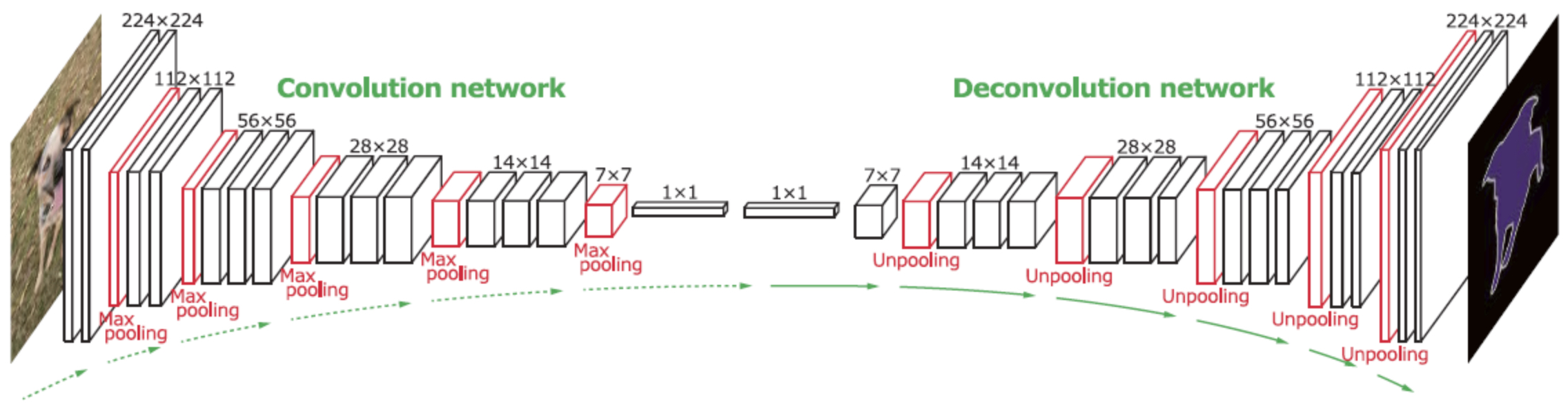
The following figure (source) shows convolution (feature extraction) compressing image features into high-level activations, and deconvolution (feature reconstruction) expanding activations back into pixel space.
Motivation: From Feature Maps Back to Input
-
A key motivation for deconvolution is to trace back from an activation map to the input image regions that triggered it. By selectively keeping only the strongest activations and back-projecting them, we reconstruct an approximate version of the input.
-
This approach is used in:
- Generative Adversarial Networks (GANs): where the generator learns to produce images from latent vectors using stacked deconvolutions. See Goodfellow et al., 2014.
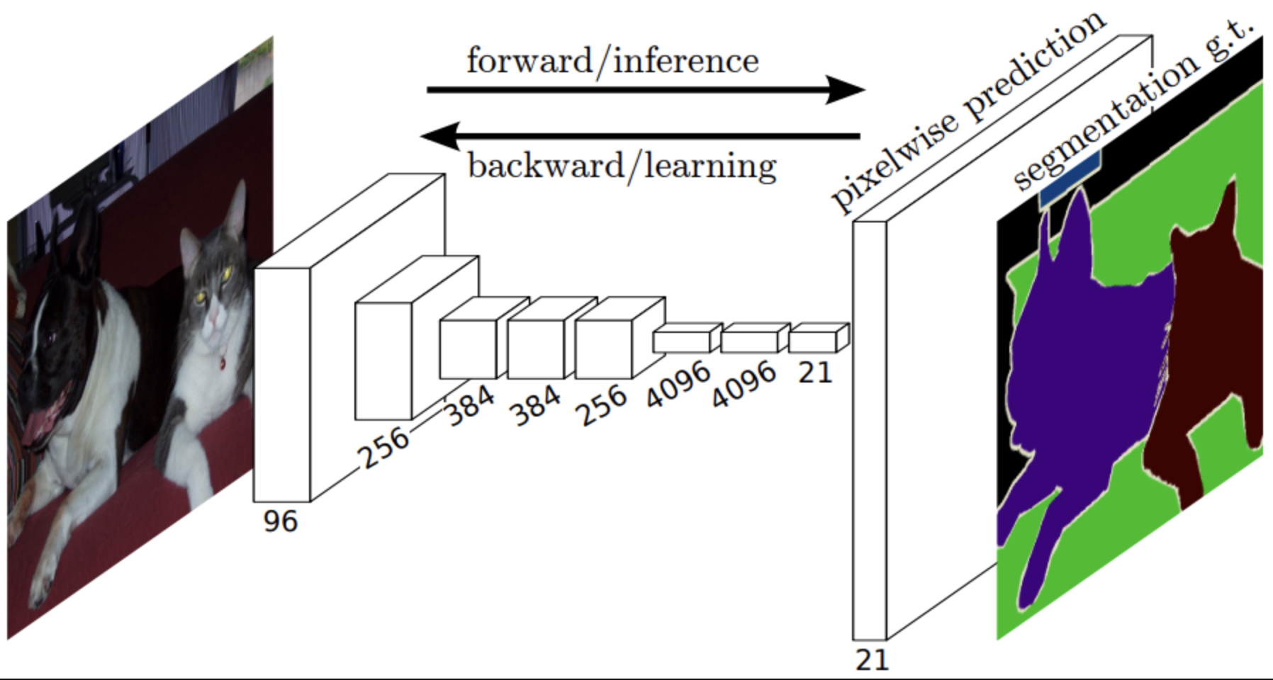
- Semantic Segmentation: where encoder-decoder architectures rely on deconvolutions to produce dense pixel-level masks. See Long et al., 2015 (Fully Convolutional Networks).
-
The following figure (source) illustrates the use of deconvolution in semantic segmentation, where the encoder compresses the input into features and the decoder reconstructs a dense mask. Specifically, figure depicts an encoder-decoder architecture for semantic segmentation, with deconvolutions expanding compressed features into pixel-level predictions.
Walkthrough with a 1D Example
- To make deconvolution concrete, let us consider a simple 1D convolution example.
Convolution
- Suppose we have an input vector of 8 elements, padded with 2 zeros on each side, forming a 12-dimensional vector:
- We apply a 1D convolution with filter size \(f = 4\) and stride \(s = 2\). The output length is:
-
Thus, the convolution is a linear transformation:
\[y = W x\]- where \(W\) is a \(5 \times 12\) matrix encoding shifted copies of the filter weights. Each element of \(y\) is a weighted sum of overlapping input patches.
Deconvolution
- The natural idea is to invert this process:
-
If \(W\) were orthogonal (so that \(W^{-1} = W^T\)), then reconstruction would be straightforward. For example, with an edge-detection filter \((w_1, w_2, w_3, w_4) = (-1, 0, 0, 1)\), the corresponding \(W\) is orthogonal, and back-projection becomes exact.
-
However, for general CNN filters, exact inversion is not efficient, leading us to more practical alternatives such as subpixel convolution.
Trick: Subpixel Convolution
-
To make deconvolution computationally feasible, we adjust the operation by inserting zeros between outputs (upsampling) before applying a convolution-like filter. This is called subpixel convolution.
-
Instead of computing \(x = W^T y\) directly, we first pad \(y\) with zeros between its entries:
- We then apply the same convolutional weights but flipped, e.g., \((w_1, w_2, w_3, w_4)\) becomes \((w_4, w_3, w_2, w_1)\). This trick preserves the efficiency of convolution while achieving the reconstruction effect of deconvolution.
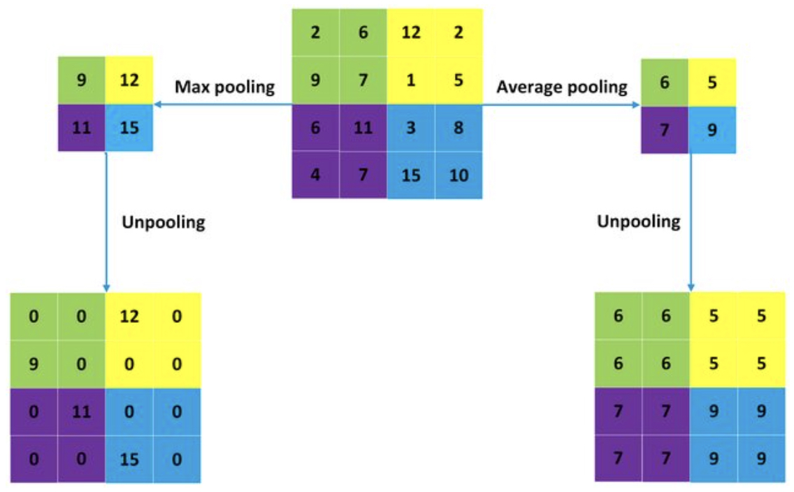
Unpooling: The Inverse of Max-Pooling
-
Another essential component in reconstruction is unpooling, the inverse of max-pooling.
- In max-pooling, we record only the maximum value within each pooling region.
-
In unpooling, we use the switches (indices of maxima) to place the values back in their original positions, filling the rest with zeros.
-
This operation restores spatial structure that was lost during pooling.
- The following figure (source) visualizes unpooling: the pooling step selects maxima, while unpooling uses the recorded positions to reconstruct a sparse activation map.
Summary
Deconvolution and unpooling extend our interpretability toolkit by enabling backward visualization and reconstruction. They are not only powerful for understanding activations but also foundational in modern architectures:
- GAN generators use stacked deconvolutions to synthesize high-resolution images.
- Semantic segmentation networks rely on encoder-decoder pipelines with deconvolution and unpooling for pixel-level predictions.
These tools thus bridge the gap between abstract feature activations and human-interpretable outputs, allowing us to “see through” the black box of CNNs.
Takeaways
-
Deep neural networks, and CNNs in particular, have reshaped the landscape of computer vision by achieving unprecedented accuracy across classification, detection, and segmentation tasks. Yet their widespread adoption hinges not only on predictive performance but also on trust and interpretability.
-
In this primer, we explored three complementary perspectives on making neural networks more transparent:
- Saliency and occlusion maps: By analyzing gradients and perturbations, we visualized which parts of the input most strongly influenced the network’s decisions. These methods reveal whether a CNN is truly focusing on relevant objects or being misled by background cues.
- Internal visualizations via gradient ascent and dataset search: By directly probing activations, we gained insight into what concepts neurons represent. Gradient ascent synthesized idealized patterns, while dataset search grounded those abstractions in real-world examples. Together, they provided a dual lens on learned features.
- Deconvolution and unpooling: By reversing the computational steps of convolution and pooling, we reconstructed inputs from activations and enabled generative tasks such as semantic segmentation and image synthesis. These methods showed how representation flows can be mapped back to human-interpretable domains.
Broader Implications
-
Beyond technical insight, these interpretability tools serve three broader purposes:
- Trustworthiness and transparency: By making the decision process explicit, they enable stakeholders to trust AI systems in sensitive domains.
- Model debugging: Visualizations expose spurious correlations or dataset biases, guiding practitioners toward cleaner data and better architectures.
- Scientific discovery: By opening the black box, we can learn how complex features are represented, offering parallels to neuroscience and cognitive science.
-
As the field advances, newer methods such as SHAP values, integrated gradients, and explainable GAN frameworks will continue to expand our interpretability arsenal. Still, the central philosophy remains the same: neural networks must not only work well but also be understood well.
Citation
If you found our work useful, please cite it as:
@article{Chadha2020InterpretabilityofNN,
  title   = {Interpretability of Neural Networks},
  author  = {Chadha, Aman},
  journal = {Distilled Notes for Stanford CS230: Deep Learning},
  year    = {2020},
  note    = {\url{https://aman.ai}}
}