CS230 • Generative Adversarial Networks
- Overview
- Motivation
- The Power of Generative Modeling
- Why GANs?
- The Generator vs. Discriminator Game
- Training GANs
- Tips to Train GANs
- Applications
- Training CycleGANs
- Takeaways
- Further Reading
- Citation
Overview
- Artificial intelligence has long been applied to predictive tasks—such as recognizing handwritten digits, detecting objects in images, or classifying medical scans. But what if neural networks could do more than simply recognize and classify? What if they could generate new data—novel images, unique audio clips, even entirely new pieces of text? This is the promise of generative models, and among them, Generative Adversarial Networks (GANs) have emerged as one of the most influential frameworks.
Motivation
-
A central question in generative modeling is whether a network can create realistic outputs it has never seen before. For example, if a neural network can classify cats versus non-cats, this implies it has captured salient features that define “cat-ness” rather than memorizing specific training examples. By the same logic, a generative model should be capable of synthesizing entirely new cat images, consistent with these learned features.
-
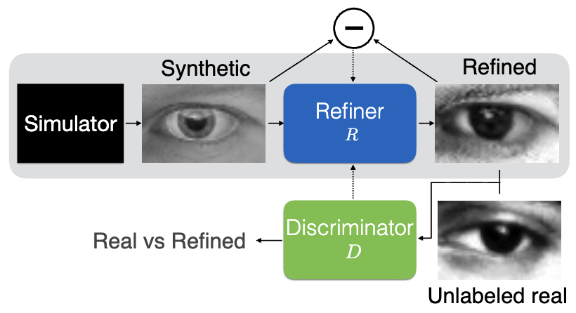
The practical motivation extends beyond curiosity. Consider robotics: training a robotic arm to localize objects on a table requires vast amounts of labeled data. Collecting real-world samples is expensive, involving physical object placement, photography, and annotation. Simulations offer a scalable alternative, generating millions of labeled synthetic images. However, networks trained purely on synthetic data often fail to generalize to real-world settings—a phenomenon known as the “sim-to-real gap.” Here, GANs can bridge the divide by generating realistic counterparts of simulated data, making virtual training transferable to physical robots.
-
The following figure (source) illustrates this principle in robotic vision, where GANs convert simulated inputs into realistic representations, enabling better generalization. It demonstrates how simulated images can be transformed into realistic counterparts using GANs, bridging the gap between virtual training environments and real-world deployment.
The Power of Generative Modeling
-
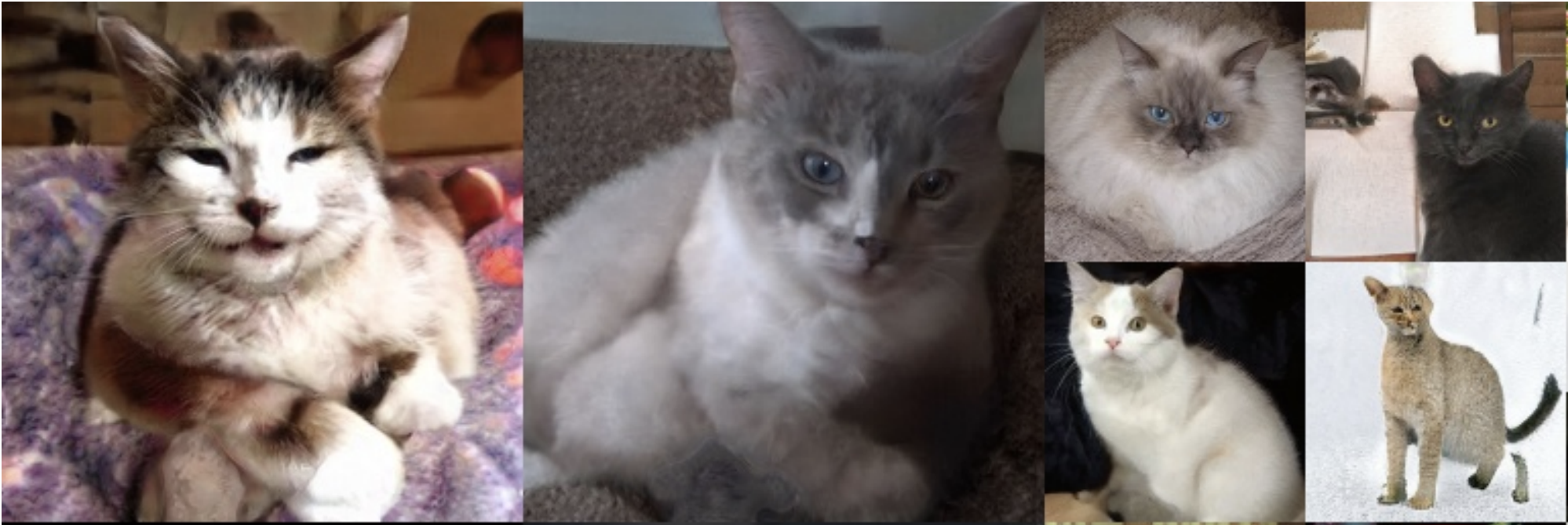
GANs are not limited to robotics. They have been used to generate realistic images of cats, cars, and even human faces—none of which exist in reality. These results, pioneered by researchers like Karras et al. (ImageNet paper), showcase the remarkable ability of GANs to model complex data distributions and synthesize high-fidelity outputs.
-
The following figures highlight the breakthrough performance of GANs:
-
The following figure shows cats generated by a GAN. None of these cats exist in reality, but they exhibit coherent textures, shapes, and poses learned from training data.
-
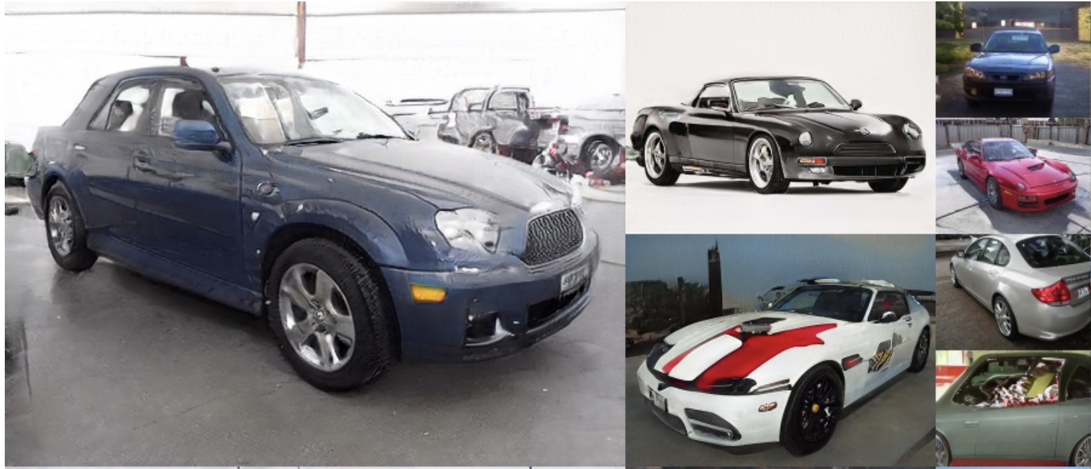
The following figure presents GAN-generated cars, revealing the model’s ability to capture rigid structures, reflections, and contextual details.
-
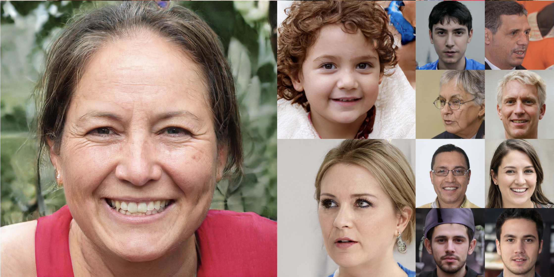
The following figure depicts GAN-generated faces, demonstrating how deeply trained models can synthesize photorealistic features indistinguishable from actual human portraits.
-
Why GANs?
-
GANs are transformative because they enable models to learn directly from data distributions without requiring explicit likelihood estimation. Traditional generative models—such as Variational Autoencoders (VAEs) or autoregressive models—struggle to balance sharpness and diversity in generated outputs. GANs, on the other hand, frame the generative task as a game between two neural networks (generator and discriminator), leading to sharper and more realistic samples.
-
In the sections that follow, we will explore:
- The fundamental architecture of GANs, including the generator-discriminator game.
- The mathematics of training GANs and optimizing adversarial objectives.
- Practical tricks to stabilize training and ensure convergence.
- Applications across domains such as image super-resolution, image-to-image translation, and medical data synthesis.
The Generator vs. Discriminator Game
- Although many generative algorithms exist, Generative Adversarial Networks (GANs) (Goodfellow et al., 2014) remain one of the most elegant formulations. They are built upon two neural networks that compete in a minimax game, where one network generates candidate data and the other judges its authenticity.
Core Components
-
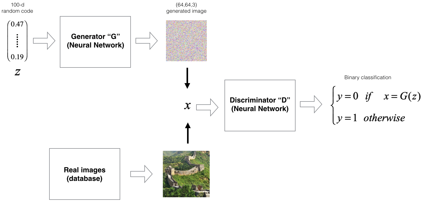
The Generator (G): The generator takes as input a random noise vector, usually denoted as \(z\), sampled from a prior distribution (e.g., uniform or Gaussian). It transforms this noise into synthetic data—such as an image. Its sole objective is to produce samples that look indistinguishable from real ones.
-
The Discriminator (D): The discriminator is a binary classifier trained to distinguish between real samples (labeled as 1) and generated samples from \(G\) (labeled as 0). Its task is to estimate the probability that a given input comes from the real dataset rather than from the generator.
The Adversarial Game
-
The interplay between \(G\) and \(D\) forms the essence of GAN training:
- \(D\) receives a mix of real samples (from the training dataset) and fake samples (from G).
- \(D\) attempts to classify them correctly, updating its parameters to minimize classification error.
- \(G\) updates its parameters so that the samples it generates can fool \(D\) into classifying them as real.
-
This iterative process resembles a cat-and-mouse game. Over time, \(G\) improves its ability to generate realistic data, while \(D\) sharpens its discrimination capacity. Ideally, the game converges when \(D\) cannot tell real from fake with better than random chance (50% accuracy).
-
The following figure illustrates this adversarial training loop by visualizing the dynamic between the generator and discriminator: \(G\) generates candidate samples from random noise, while \(D\) attempts to classify them as fake or real, iteratively refining both networks.
Mathematical Formulation
-
Formally, the generator and discriminator engage in the following minimax optimization problem:
\[\min_G \max_D V(D, G) = \mathbb{E}_{x \sim p_{\text{data}}(x)}[\log D(x)] + \mathbb{E}_{z \sim p_z(z)}[\log (1 - D(G(z)))]\]-
where:
- \(p_{\text{data}}(x)\) is the true data distribution.
- \(p_z(z)\) is the prior distribution of the latent vector z.
- \(D(x)\) represents the discriminator’s estimate that sample x is real.
- \(G(z)\) is the generator’s synthetic sample corresponding to latent input z.
-
-
Intuitively:
- \(D\) aims to maximize this function by assigning high probability to real samples and low probability to generated ones.
- \(G\) aims to minimize it by producing samples such that \(D(G(z))\) is close to 1.
-
This adversarial dynamic captures the equilibrium point of the system, where the generated distribution matches the real data distribution.
Sampling from the Generator
-
The input noise vector \(z\) is critical: it injects randomness, ensuring diversity in generated samples. By default, \(z \sim \mathcal{N}(0, I)\) or \(z \sim \text{Uniform}(-1,1)\). Through the learned mapping \(x = G(z)\), GANs discover complex transformations from latent noise to structured outputs.
-
Later, we will see how modifying the structure of \(z\) allows for controllable generation (e.g., adjusting facial attributes or object styles).
Training GANs
- Training a GAN involves optimizing two cost functions simultaneously: one for the discriminator (D) and one for the generator (G). Unlike standard supervised learning, this is a two-player game where improvements in one player force improvements in the other.
Discriminator’s Cost Function
-
The discriminator is a binary classifier whose goal is to assign high probability to real samples and low probability to generated ones. Using binary cross-entropy, its cost function can be written as:
\[J^{(D)} = -\frac{1}{m_{\text{real}}}\sum_{i=1}^{m_{\text{real}}} \log (D(x_{\text{real}}^{(i)})) - \frac{1}{m_{\text{gen}}}\sum_{i=1}^{m_{\text{gen}}} \log (1 - D(G(z^{(i)})))\]-
where:
- \(m_{\text{real}}\) is the number of real examples in a batch.
- \(m_{\text{gen}}\) is the number of generated examples.
- \(x_{\text{real}}^{(i)}\) is a real training sample.
- \(G(z^{(i)})\) is a generated sample.
-
Here, \(D(x_{\text{real}})\) should be close to 1, while \(D(G(z))\) should be close to 0.
-
Generator’s Cost Function
- The generator’s goal is to fool the discriminator. Its success is measured by how often \(D\) misclassifies fake samples as real. The standard generator cost is:
- Unlike the discriminator, the generator does not directly use real samples in its loss—it only learns through the discriminator’s feedback.
Two-Step Optimization Process
-
Training proceeds iteratively in two alternating steps:
-
Update the discriminator (D):
- Feed a mini-batch of real samples.
- Feed a mini-batch of fake samples from \(G\).
- Compute \(J^{(D)}\), then backpropagate to update discriminator parameters \(W_D\).
-
Update the generator (G):
- Sample noise vectors \(z\).
- Generate samples \(G(z)\).
- Compute both \(J^{(D)}\) (on fake samples) and \(J^{(G)}\).
- Backpropagate through \(G\) to update its parameters \(W_G\).
-
-
This alternating procedure ensures that both networks improve in tandem.
-
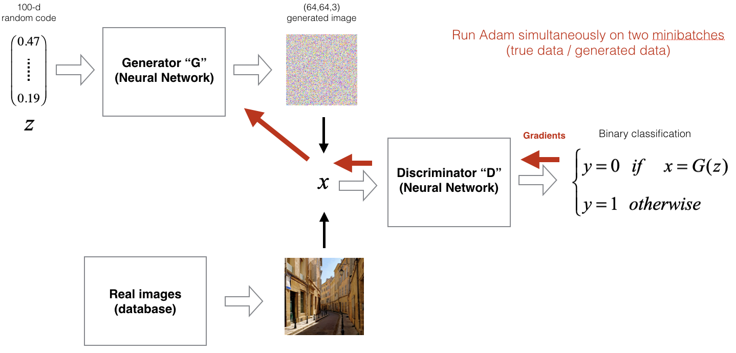
The following figure shows the GAN training process, where the generator and discriminator are optimized iteratively, each improving in response to the other’s progress.
Convergence
-
If training is successful, the distribution of generated samples \(p_g(x)\) will converge to the true data distribution \(p_{\text{data}}(x)\). At this Nash equilibrium:
- The discriminator cannot distinguish real from fake better than chance, i.e. \(D(x) \approx 0.5\).
- The generator produces highly realistic samples, effectively fooling D.
-
Goodfellow’s original paper GANs, 2014 showed mathematically that this equilibrium is guaranteed under ideal conditions with infinite capacity models and perfect optimization. In practice, however, optimization difficulties and instability often prevent reaching equilibrium.
-
For hands-on exploration, you can study this implementation in Keras, which provides a simple baseline to experiment with GAN training.
Tips to Train GANs
- In practice, training GANs is notoriously unstable. Unlike standard supervised learning, where the optimization objective is fixed, GANs involve two networks with competing goals. If one player becomes too strong relative to the other, training collapses. Over the years, researchers have developed a series of practical tricks to stabilize GAN training and improve sample quality.
Trick 1: Using a Non-Saturating Cost
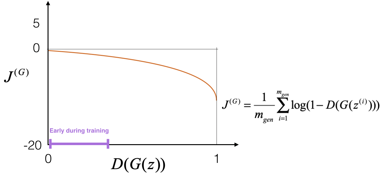
- One of the earliest insights was that the standard generator cost function,
-
… can saturate early in training. This happens because when the generator is poor (e.g., producing noise), the discriminator easily detects fake samples, leading to \(D(G(z)) \approx 0\). In this regime, the gradient signal for \(G\) becomes very small, slowing learning drastically.
-
The following figure visualizes this problem. It shows the saturating cost curve, where the generator’s gradient becomes very small when \(D(G(z)) \approx 0\), hindering learning in early stages.
-
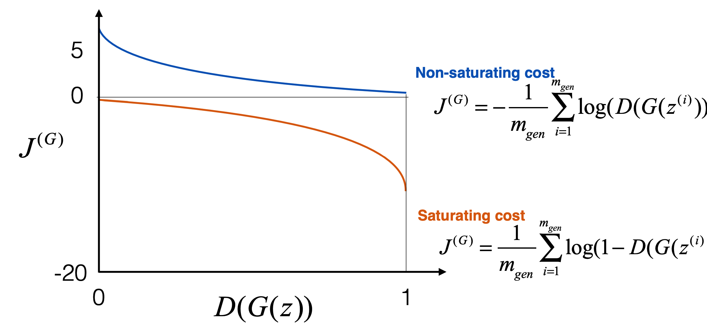
To address this, Goodfellow proposed the non-saturating trick, where instead of minimizing \(\log(1 - D(G(z)))\), the generator maximizes \(\log(D(G(z)))\). Equivalently, the cost becomes:
-
This redefinition provides a stronger gradient when the discriminator is confident, allowing the generator to improve even if it initially produces poor outputs. Importantly, this trick does not alter the equilibrium point (where \(D(G(z)) = 0.5\)).
-
The following figure compares the saturating and non-saturating cost functions. The non-saturating formulation provides stronger gradients early in training, enabling faster generator improvement.
-
For a more detailed explanation, see Goodfellow’s NIPS 2016 tutorial, which remains a classic reference.
Trick 2: Keeping the Discriminator Up-to-Date
-
Another challenge arises when the generator temporarily gains the upper hand. If the discriminator becomes too weak (i.e., \(D(G(z)) \approx 1\) for most fake samples), the generator again stops receiving useful gradient signals.
-
A common remedy is to train the discriminator more frequently than the generator. For example, one can update \(D\) \(k\) times per update of G, with \(k > 1\). This ensures that \(D\) remains a strong adversary, continually pushing \(G\) to improve.
-
This strategy maintains the adversarial balance:
- If \(D\) is too weak, \(G\) improves without constraint, leading to unrealistic samples.
- If \(D\) is too strong, \(G\) cannot learn, as gradients vanish.
- Proper balance ensures both players improve in tandem.
Other Tricks
-
The research community has developed many more techniques for stabilizing GAN training, including:
- Gradient penalty methods (e.g., WGAN-GP).
- Label smoothing and noisy labels.
- Feature matching and minibatch discrimination.
- Architectural adjustments such as spectral normalization.
-
For a comprehensive collection of these hacks, see Soumith Chintala’s GAN hacks repository, which remains a valuable resource for practitioners.
Applications
-
GANs have evolved into one of the most versatile tools in machine learning, with applications across domains as diverse as computer vision, healthcare, robotics, and creative arts. They are not only a playground for exploring generative modeling but also practical engines of innovation.
-
Here we highlight a selection of their most impactful applications.
Operation on Latent Codes
-
GANs operate in a latent space, where random vectors \(z\) are mapped to realistic data samples by the generator \(G\). Interestingly, this latent space is not arbitrary—it encodes semantically meaningful directions. By manipulating these codes, one can perform structured edits on generated images.
-
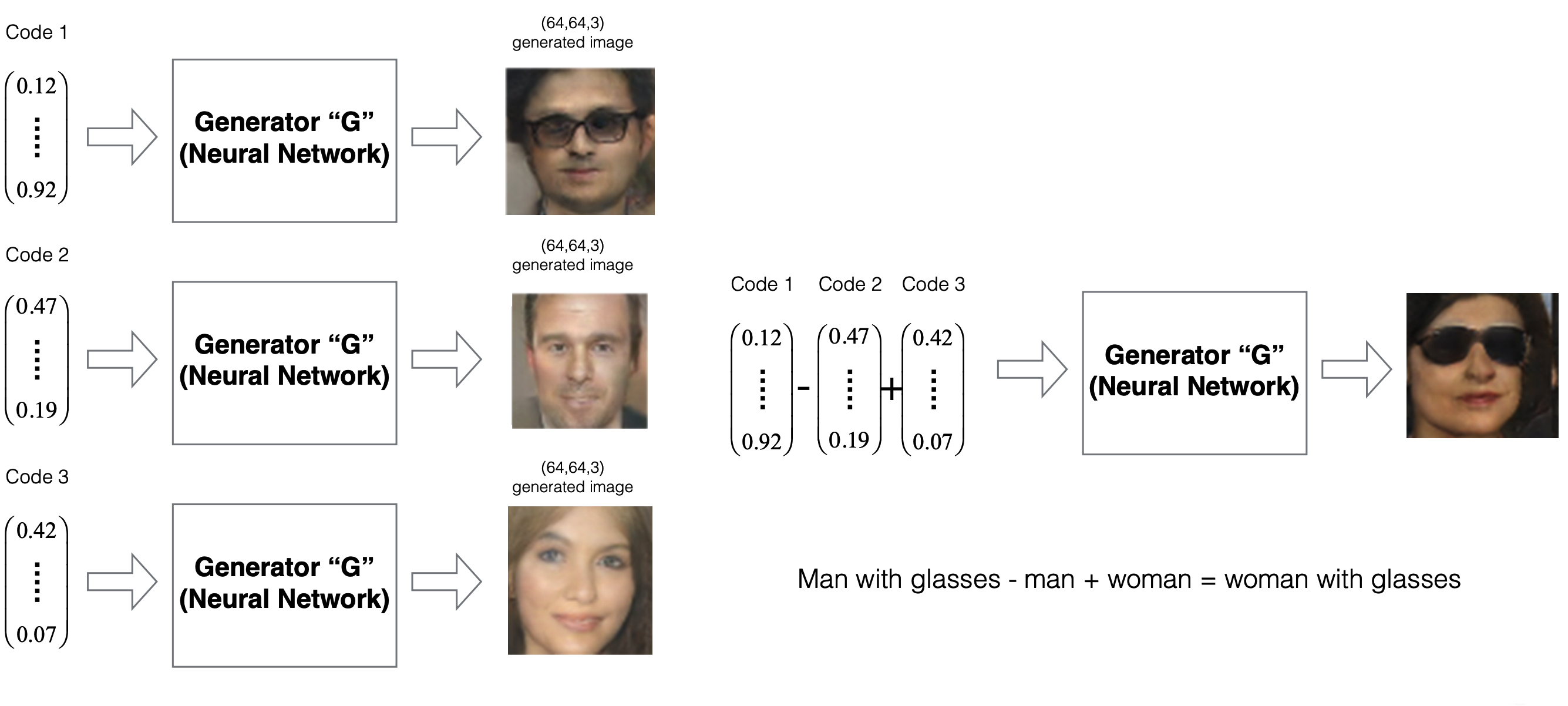
Radford et al. (DCGAN, 2015) demonstrated that arithmetic on latent codes corresponds to interpretable changes in outputs. For example:
-
When fed into the generator, this yields an image of a woman wearing glasses—a striking example of disentangled representation learning.
-
The following figure illustrates such latent space manipulations. It shows how arithmetic in the latent space of a GAN can produce semantically meaningful transformations, such as adding or removing glasses from generated faces.
Generating Super-Resolution (SR) Images
-
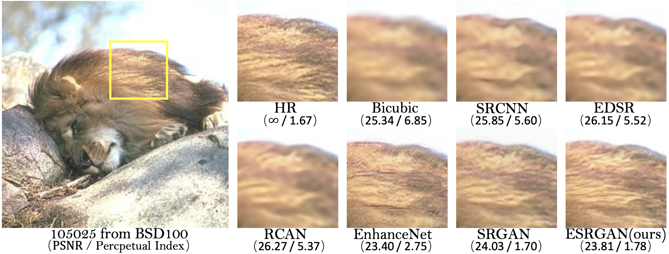
Another major success of GANs lies in super-resolution (SR)—the task of reconstructing high-resolution images from low-resolution inputs. Traditional interpolation methods (e.g., bicubic) often blur details. GAN-based approaches, however, can hallucinate fine textures and sharper boundaries.
-
Applications include:
- Surveillance and vehicle identification.
- Medical imaging for enhanced tissue visualization.
- Biometric recognition such as face or fingerprint reconstruction.
-
The following figure compares outputs from different super-resolution algorithms, with GAN-based models recovering sharper details and textures closer to the ground-truth. The leftmost image is the ground truth; GAN-based methods produce reconstructions closer to it than conventional techniques:
-
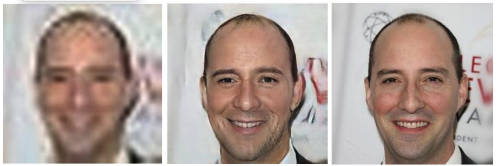
More impressively, student projects at Stanford’s CS230 have pushed SRGAN approaches to new heights. In the example below, a 32×32 low-resolution input is transformed into a 256×256 output that closely matches the high-resolution ground truth.
-
The following figure shows super-resolution in action: starting from a 32×32 low-resolution input, a GAN reconstructs a high-fidelity 256×256 output comparable to the original image.
-
For seminal works in this area, see Ledig et al., 2016 and Wang et al., 2018.
Image-to-Image Translation via CycleGANs
-
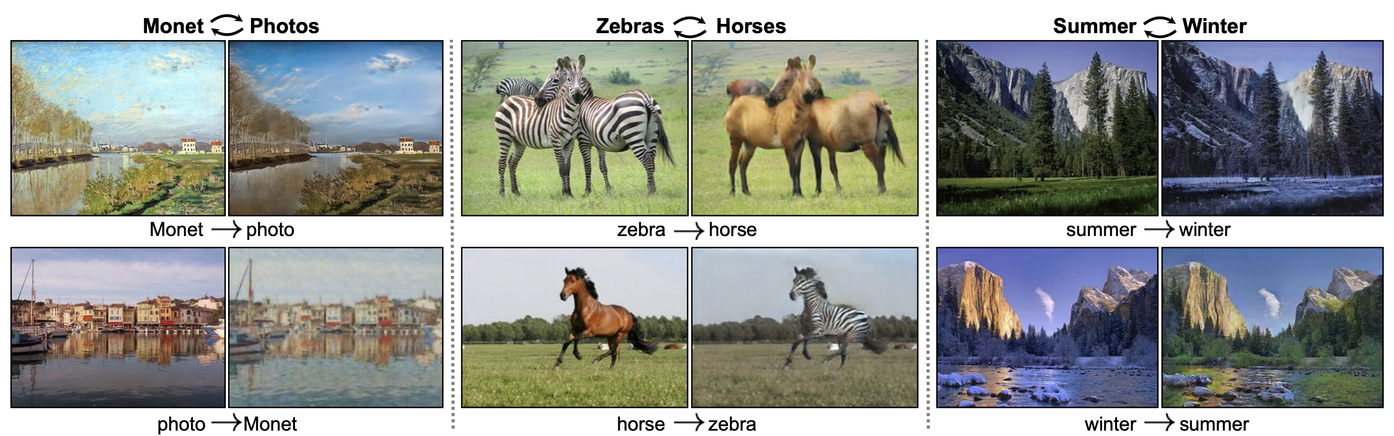
GANs also excel at translating images between domains. CycleGANs (Zhu et al., 2017) enable mappings such as:
- Horses ↔ Zebras
- Apples ↔ Oranges
- Summer ↔ Winter scenes
-
Crucially, CycleGANs do not require paired datasets (e.g., the same horse photo with a corresponding zebra photo). Instead, they enforce cycle consistency: translating from domain A to B and back to A should recover the original image.
-
The following figure demonstrates CycleGAN outputs where animals and environments are translated convincingly across domains: horses become zebras, apples turn into oranges, and summer landscapes transform into winter scenes.
-
This is achieved with two pairs of generator-discriminator networks \((G_1, D_1)\) and \((G_2, D_2)\), trained jointly with adversarial and cycle-consistency losses. Such architectures have been applied to tasks like medical imaging (e.g., CT-to-MRI translation), satellite image conversion, and artistic style transfer.
-
GANs have also found use in privacy-preserving medical data generation (Yale University study, 2018), language modeling, and even cryptography (Chi et al., 2018). Their adaptability across modalities makes them a central pillar in modern AI research.
Training CycleGANs
- Unlike vanilla GANs, which learn to map random noise vectors to realistic samples, CycleGANs Zhu et al., 2017 tackle the harder problem of translating between two structured domains without requiring paired training data.
The Two-Domain Setting
-
We are given:
- Domain H (e.g., horses, summer scenes, CT images).
- Domain Z (e.g., zebras, winter scenes, MRI images).
-
The task is to learn mappings:
- \(G_1: H \to Z\) (e.g., horse → zebra).
- \(G_2: Z \to H\) (e.g., zebra → horse).
-
Each mapping is paired with its own discriminator:
- \(D_1\), which distinguishes between real zebras and generated zebras.
- \(D_2\), which distinguishes between real horses and generated horses.
-
This gives us two generator-discriminator games that operate simultaneously.
Adversarial Losses
-
Each generator-discriminator pair has its own adversarial loss, just like in standard GANs.
-
For \(D_1\) (zebra domain):
- For \(G_1\):
- Similarly, for \(D_2\) (horse domain):
- For \(G_2\):
- These adversarial losses encourage each generator to produce outputs indistinguishable from real samples in the target domain.
Cycle-Consistency Loss
- Adversarial losses alone are insufficient: a generator could map all horses to a single zebra image and still fool the discriminator. To prevent this collapse, CycleGAN introduces the cycle-consistency constraint:
-
This ensures that translating an image from one domain to the other and back again reconstructs the original image. The cycle loss is given by:
\[J^{\text{cycle}} = \mathbb{E}_{h \sim p_H(h)} \big[ \| G_2(G_1(h)) - h \|_1 \big] + \mathbb{E}_{z \sim p_Z(z)} \big[ \| G_1(G_2(z)) - z \|_1 \big]\]- where, the \(L_1\)-norm enforces pixel-level similarity, promoting faithful reconstruction of content and structure.
Identity Loss (Optional Extension)
- In some settings, an identity loss is also added to encourage generators to preserve features when inputs are already in the target domain:
- This helps preserve colors, backgrounds, and non-changing structures across translations (e.g., sky colors when turning summer into winter).
Overall Objective
-
The total loss is a weighted sum:
\[J^{\text{total}} = J^{(G_1)} + J^{(G_2)} + \lambda_{\text{cycle}} J^{\text{cycle}} + \lambda_{\text{id}} J^{\text{id}}\]- where \(\lambda_{\text{cycle}}\) and \(\lambda_{\text{id}}\) control the importance of cycle-consistency and identity preservation.
Training Dynamics
-
Training involves:
- Updating discriminators \(D_1\) and \(D_2\) to distinguish real from fake in each domain.
- Updating generators \(G_1\) and \(G_2\) to fool their respective discriminators while satisfying cycle-consistency.
- Iterating until the generators produce convincing translations that preserve essential structure.
-
This architecture has been applied to numerous domains, including:
- Translating artworks into photographs and vice versa.
- Medical imaging conversions (CT ↔ MRI).
- Satellite image ↔ map translations.
Takeaways
-
Adversarial Training as a Game
- GANs introduced the concept of learning through competition, where the generator and discriminator continuously adapt to one another.
- This interplay, while powerful, also makes training delicate and requires careful balancing through tricks like non-saturating loss and frequent discriminator updates.
-
Versatility Across Domains
- From photorealistic face generation to medical data synthesis, GANs have found applications across science, engineering, and art.
- Latent code arithmetic reveals structured representation learning, while CycleGANs demonstrate how unpaired translation can solve real-world domain adaptation problems.
-
Challenges in Stability and Evaluation
- Training instability, mode collapse (where the generator produces limited varieties of outputs), and lack of reliable evaluation metrics remain persistent challenges.
- While metrics such as Inception Score (IS) and Fréchet Inception Distance (FID) provide partial insight, the field still lacks a universally accepted standard.
Further Reading
- A Style‑Based Generator Architecture for Generative Adversarial Networks (StyleGAN) — Tero Karras, Samuli Laine, and Timo Aila, CVPR 2019.
- Generative Adversarial Networks (GANs) — Ian J. Goodfellow et al., 2014.
- Adam: A Method for Stochastic Optimization — Diederik P. Kingma and Jimmy Ba, 2014
- Photo‑Realistic Single Image Super‑Resolution Using a Generative Adversarial Network (SRGAN) — Christian Ledig et al., 2016.
- ESRGAN: Enhanced Super‑Resolution Generative Adversarial Networks — Xintao Wang et al., 2018 ([WIRED][4])
- Privacy‑Preserving Generative Deep Neural Networks Support Clinical Data Sharing — Brett K. Beaulieu‑Jones et al., 2017.
- Generative Adversarial Text to Image Synthesis — Scott Reed et al., 2016.
- Unsupervised Image‑to‑Image Translation Networks (CycleGAN) — Ming‑Yu Liu, Thomas Breuel, Jan Kautz, 2017.
- Learning Beyond Human Expertise with Generative Models for Dental Restorations — Jyh‑Jing Hwang et al., 2018.
- Unsupervised Cipher Cracking Using Discrete GANs — Aidan N. Gomez et al., 2018.
- Unsupervised Representation Learning with Deep Convolutional Generative Adversarial Networks (DCGANs) — Alec Radford, Luke Metz, Soumith Chintala, 2015.
- Fast Super‑Resolution for License Plate Image Reconstruction — Yuan Jie, Du Si‑dan, Zhu Xiang, 2008.
- Human Portrait Super‑Resolution Using GANs (CS230 project report) — Yujie Shu, 2018.
- Unpaired Image‑to‑Image Translation using Cycle‑Consistent Adversarial Networks (CycleGAN original paper) — Jun‑Yan Zhu, Taesung Park, Phillip Isola, Alexei A. Efros, 2017.
Citation
If you found our work useful, please cite it as:
@article{Chadha2020GANs,
  title   = {Generative Adversarial Networks},
  author  = {Chadha, Aman},
  journal = {Distilled Notes for Stanford CS230: Deep Learning},
  year    = {2020},
  note    = {\url{https://aman.ai}}
}