CS230 • Deep Learning Intuition
- Primer
- Day-and-night Classification
- Face Verification and Recognition
- Neural Style Transfer (Art Generation)
- Trigger-word Detection
- App Implementation
- In this topic, we will learn tips and tricks to:
- Analyze a problem from a deep learning approach
- Choose an architecture
- Choose a loss and a training strategy
-
by going through the following problems:
-
Day-and-night Classification
-
Face Verification and Recognition
-
Neural Style Transfer (Art Generation)
-
Trigger-word Detection
-
App Implementation
-
Primer
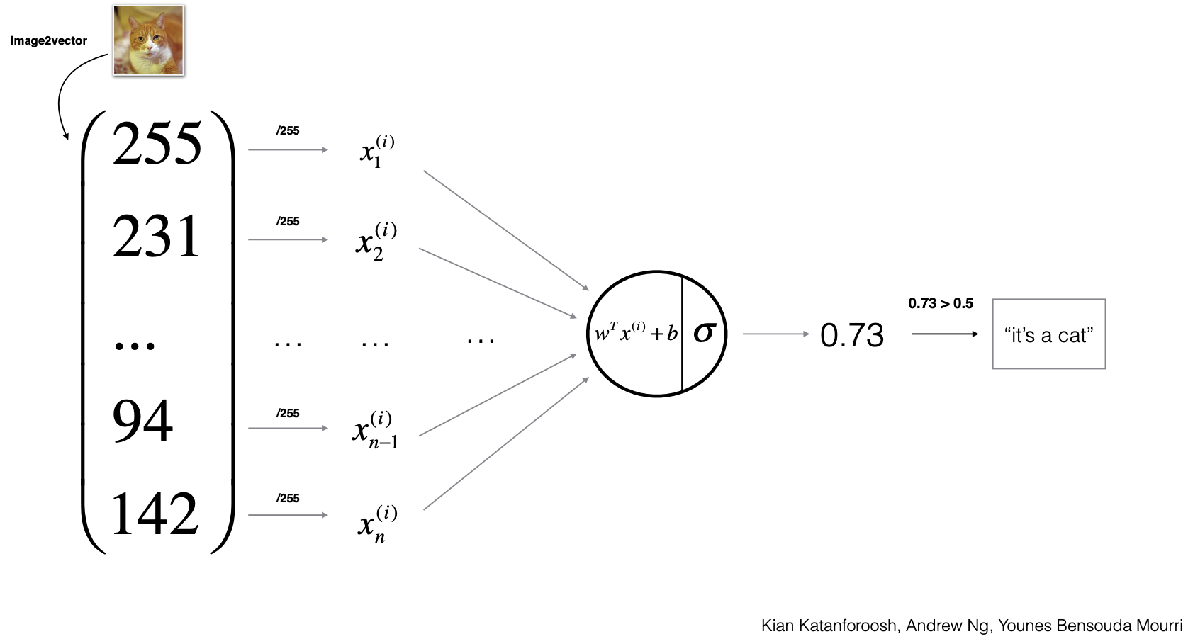
- We are already familiar with the Logistic Regression setup for a binary classifier for cat. Now let’s suppose we want to expand the model to a multi-class classifier so that it can classify cat, dog and giraffe.
- Architecture: Modify the model so that it has 3 neurons, each classifying cat, dog or giraffe.
- Data: Add dog and giraffe data. Use one-hot encoding for the label if there’s at most a single class in the image, or multi-hot encoding for the label if there can be multiple classes in a image at the same time.
- Activation function choice:
- Sigmoid: outputs of the neurons are independent. So there could be more than one probability that is greater than the threshold.
- Softmax: outputs of the neurons are dependent, sum up to 1, and each indicate what’s the probability of one class versus another. A good choice if we constrain each image to have only one class.
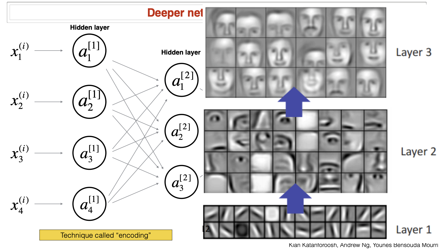
- In deeper neural networks, the earlier layers contain low-level information such as edges. Higher level layers will usually contain more complex features of regions such as eyes, noses, and faces. These lower-dimensional representations of the data are called encodings.
Day-and-night Classification
- Let’s start with an easy warm-up. Here, our Goal is to classify a given image as taken “during the day” (0) or “taken during the night” (1).
- Data: Images of nights and days could be found easily on the Internet. Therefore, we can start with 10,000 images, and increase the size later if needed. Split? Bias?
- Input: Next, we need to decide about the size of our input image. One way to think about this is by comparing the complexity of the task with previous tasks that we have worked on. Earlier in this course, you trained a cat classification model with an input size of 64x64x3. Day’n’Night classification seems like an easier task; thus, the same input size -providing the same level of detail- would be a good starting point.

- Output: As mentioned above, the output of the model should be 0 or 1, for day and night respectively. Hence, Sigmoid function would be a good fit for our final layer activation function.
- Architecture: Considering our cat classification model, by which we achieved a high accuracy using a 4-layer neural network, a shallow network should do the job pretty well.
- Loss: Since the last layer will be using Sigmoid activation function, cross-entropy loss function will be set as model’s objective: \(L = -[y \log(\hat{y}) + (1-y) \log(1-\hat{y})]\)
Face Verification and Recognition
-
A school wants to use face verification for validating student ID’s in facilities (dining halls, gym, etc.). Person requesting access will swipe his/her student ID, providing the model with the name and label to locate student’s stored image on the database. Model will then compare his current picture (captured by a camera at the location) with the saved image, to verify his/her ID.
- Data: The school has access to a dataset with one picture for every student labeled with their name.
- Input: Compared with the previous problem, face recognition is a more complicated task. Model should be robust to changes in position of the face, brightness of the picture, facial details (e.g. beard or sunglasses), etc. Therefore, the model must be provided with more details on the face, leading to a higher resolution for the inputs. 412x412x3 would be a good place to start.
- Output: Output of the model should be “ID verified” (1) or “ID not verified” (0). Thus, Sigmoid function would be the ideal activation for the final layer.
- Architecture: A simple solution would be to compute pixel-by-pixel distance between the two images, and predict “ID verified” (1) if the distance is less than a threshold. However, this model will not perform well due to the following issues:
- Background lighting differences
- Person wearing make-up or having a beard
- ID photo being outdated
- …
- A better solution is to train a deep network to encode information about a picture in a vector. We can then, gather all student faces’ encodings in a database. Given a new picture, we compute its distance with the encoding of the card holder. If the distance is less than a threshold, the model predicts “ID verified” (1).
- Now, let’s consider a more complicated task, Face Recognition. Here, the goal to recognize the face of the person: given only an image, the model should verify if the person is indeed an student in the database or not. We need more data (multiple pictures of same people) so that our model can understand how to encode. We can use public face datasets for our training.
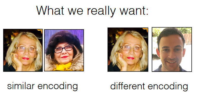
- What we want is for our model to generate similar encodings for different pictures of the same person, and different encodings, when the two pictures belong to different people.
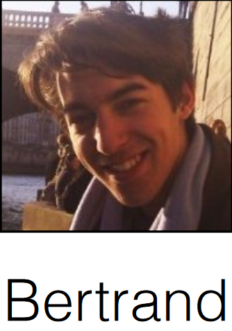
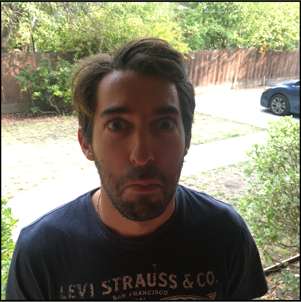
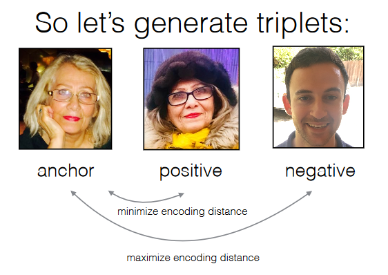
 - Our training approach is as follows. Triplets are generated containing an anchor image, an image similar to the anchor, positive, and one different from it, negative. Optimization goal is defined to minimize encoding distance between anchor and positive while maximizing encoding distance between anchor and negative.
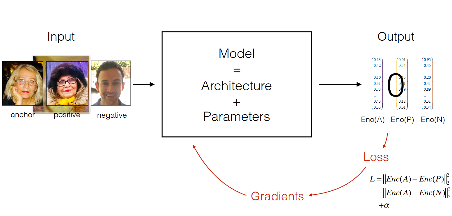
- Loss: Objective function takes the following form. \(L = {\|\|Enc(A) - Enc(P)\|\|_2}^2 - {\|\|Enc(A) - Enc(N)\|\|_2}^2 + \alpha\) Note that a constant, \(\alpha\), is added to the loss function in order to make sure the model avoids using zero function as encoding.
- Data: The school has access to a dataset with one picture for every student labeled with their name.
-
Our final model is as below.
Neural Style Transfer (Art Generation)
-
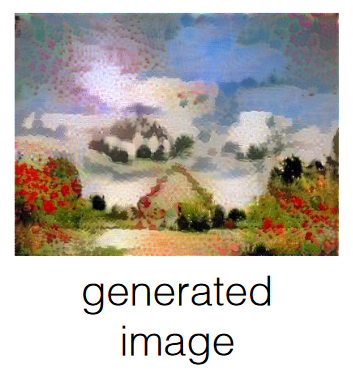
In Neural Style Transfer, our goal is to modify the style of the input image to match that of the style image, so that it looks beautiful!
-
Data: Let’s assume that we have access to any required data, and move on to the next part.
-
Input: Content and style images are given as input.
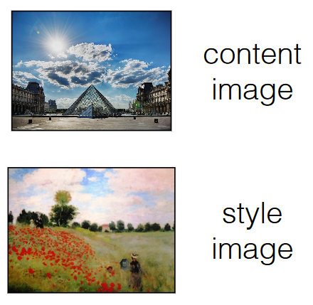
- Output: The output is the content image as if it was painted with the same style as in the style image.
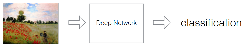
- Architecture: Note that we need the model to understand the image very well. Research has shown that models trained on images, see (or understand) contents of an image, meaning contours and curves, in the earlier layers, while information about style is captured (or understood) in the deeper layers. Thus, we use an existing model trained on ImageNet to retrieve such information from the image.
-
When this image forward propagates, we can get information about its content and its style by inspecting the layers.
-
For more information, refer to Leon A. Gatys, Alexander S. Ecker, Matthias Bethge: A Neural Algorithm of Artistic Style, 2015
-
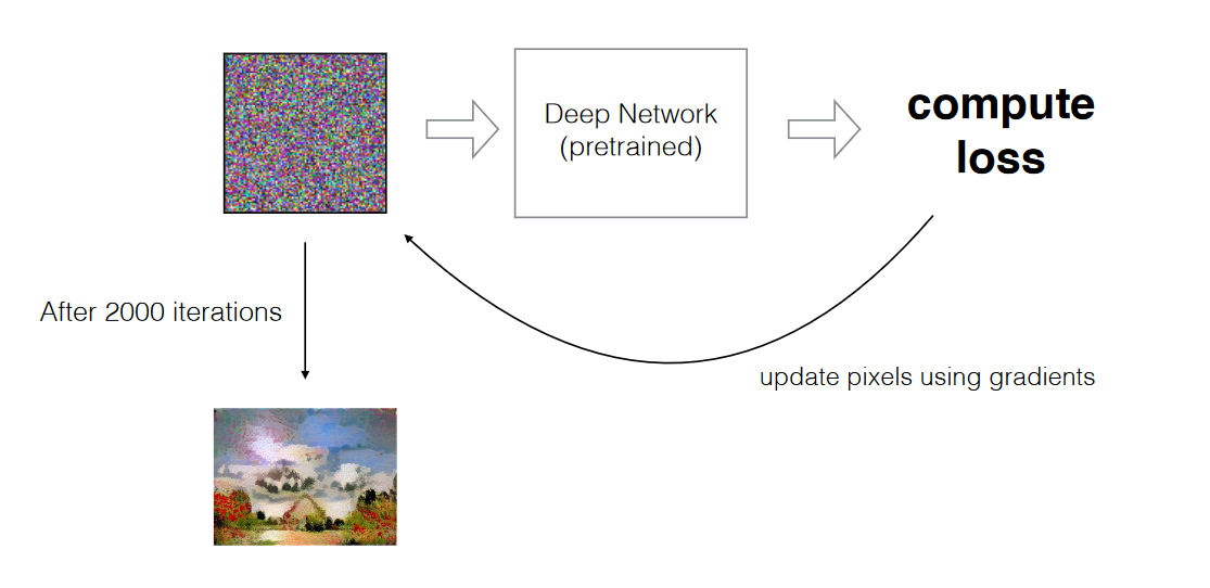
Loss: Objective function should take the following form: \(L = {||Content_C - Content_G||_2}^2 - {||Style_S - Style_G||_2}^2\)
- where, \(G\) represents the target image, \(C\) denotes content image, and \(S\) denotes style image.
- Note that here, we are not learning parameters by minimizing $$L$. We are learning an image!
-
Trigger-word Detection
-
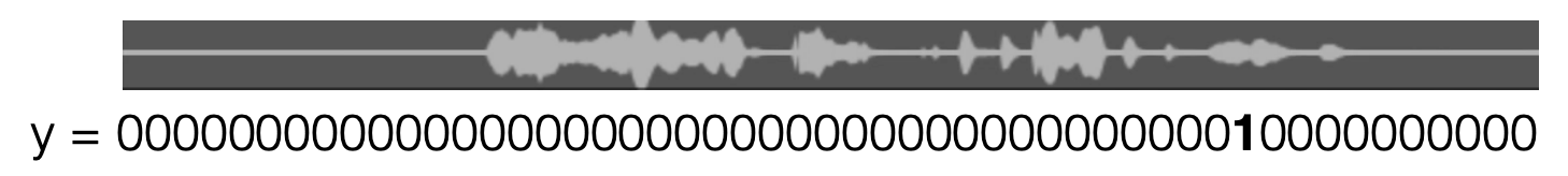
Given 10-second audio speech, we want to detect the word “activate”.
-
Data: A bunch of 10s audio clips. Distribution of positive (“activate”) and negative words (all other words) should be balanced. And should include data of different accent, gender, age, etc.
-
Input: x = 10s audio clips from above. For a good resolution/sample rate choice, we can consult experts in speech.
-
Output: We can use Sigmoid for activation at every timestep. And we have different ways for what the model should output:
- \(y = 0\) or \(y = 1\): this indicates if a 10s audio clip contains the trigger word or not. But if we set it up this way, we need gigantic amount of data to train the model.
- \(y = 000 \ldots 1 \ldots 000\): in this method, we output 1 where the audio has the trigger word. Compared to the first method, we will need less data.
- \(y = 000 \ldots 111 \ldots 000\): however, the second method will have highly unbalanced data since there’s one 1 and 0 everywhere else. To mitigate this problem, we can add in more 1s where the trigger word is.
-
Architecture: RNN (which will be covered later in the course).
-
Loss: Since there are two classes, binary cross entropy at every timestep should be good. Another way is to use triplet loss as we do for Face Recognition.
- For this project, it is important to use a strategic data collection/labeling process. Instead of going out and collecting 10s audio clips of people saying different words, we can collect people saying positive words, negative words, and background noises separately, and later synthesize the data by overlaying positive and negative words onto the background noises. This way we also have a more automated way of labeling the data – where you insert the positive word is where the label should have 1s, and 0 everywhere else. Otherwise, we would have to go through all the 10s clips and manually label them.
-
App Implementation
- We have been building an algorithm to classify cats. Now suppose we want to ship it with a phone app, i.e. we want to build an app with which you can take a picture and the app tells you if there’s a cat in the picture or not.
- There are two ways of doing it and each with its own advantages:
- Server-based: server holds the model architecture and learned parameters. The phone takes a picture, sends it to the server, the server runs the picture through the model, gets an output, and sends the output back to the phone.
- Advantage:
- App is light weight: model architecture and parameters are on server server.
- App is easy to update: you only need to modify or retrain the model on the server.
- Advantage:
- On-device: Everything happens on the device! The device holds the model architecture and learned parameters.
- Advantage:
- Faster prediction: your phone doesn’t need send requests to server and wait for a response from server.
- Works offline: your app works even when there’s no internet.
- Advantage: