CS230 • Deep-Reinforcement Learning
- Motivation
- A gentle introduction to Reinforcement Learning
- Deep Q-Learning
- Applications of Deep Q-Learning
- Training Tricks
- Exploration vs. Exploitation
- Advanced Topics
-
In this topic, we will see how we can use Deep Learning techniques to solve Reinforcement Learning (RL) problems.
-
But first, what is Reinforcement Learning? Reinforcement Learning is an area of Machine Learning. It is about automatically learning to make the best sequences of decisions to achieve a goal.
-
In previous topics, we saw how Deep Neural Networks are universal function approximators. Today we will see how we can leverage this property in RL problems. This is what we call Deep-Reinforcement Learning.
Motivation
- To motivate our interest, we will start by having a look at two major success stories in the Deep-RL field.
AlphaGo
-
AlphaGo became widely known as the first computer computer program to be able to beat a professional player at the game of Go. This accomplishment attracted a vast public interest. A documentary film was even made around the event.
-
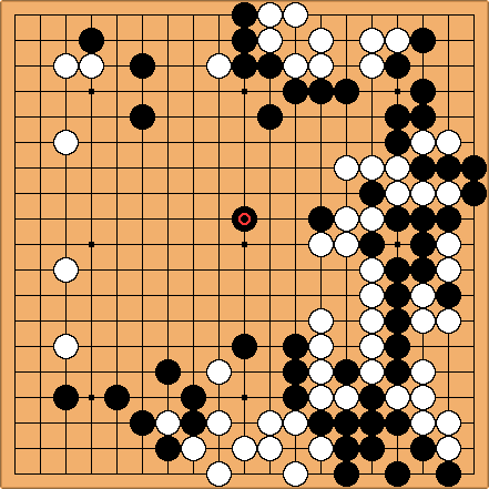
What is Go? Go is an abstract strategy board game which opposes two competitive players. The aim is to surround more territory than the opponent.
- What are the basic rules of the game of Go?
- the standard Go board is composed of a \(19 \times 19\) line grid;
- each player is assigned a set of stones (black stones for one player, white stones for the other);
- players alternatively put one of their stones at grid intersections to surround the other player’s stones;
- at the end, the player with the biggest territory wins.
- If you want to know more about Go, you can read the Wikipedia article on Go. Here’s a Go board:
- A little bit of history:
- 1997: IBM’s computer Deep Blue beat world chess champion Garry Kasparov.
- 2016: Deep Mind’s program AlphaGo beat 9-time professional player Lee Sedol.
-
Why such a time gap between the two events? Solving the game of Go is much more challenging than solving Chess. This is mainly because the state space is a lot bigger (see below).
-
How could you try to solve the game of Go using conventional Deep Learning techniques?
- Here is one possible way to define a dataset:
- input = current state of the board: positions and colors of the stones placed on the board;
- label = best next move: given by a professional player.
-
There are three major problems that would make this system unlikely to perform well on this task:
1) The input space is huge. There are \(3^{11 \times 11}\) different configurations of the board. The dataset can only cover a very small fraction of the possible inputs, it is unlikely that the algorithm will generalize well to unseen situations. 2) The model can only be as good as the professional player that made the labels. Here the labels are not the ground truth i.e. the best next moves. Our model cannot achieve super-human performances. 3) Only short term understanding. The model only plan one move ahead, it does not have any long term strategy. The issue is that an action that may not seem as the best move according to the previous one-step model might actually increase the probability of winning.
-
To solve these issues, Reinforcement Learning techniques were used. RL is well-suited in this setup because the labels we are really interested in are delayed labels: either 1 = ‘winning the game’ or 0 = ‘losing the game’. RL allow to learn a strategy to achieve long term goals.
- If you want to learn more about AlphaGo, you can read the corresponding paper from DeepMind.
Human Level Control through Deep Reinforcement Learning
-
This refers to a specific algorithm that was conceived to achieve super-human performances on a set of video games.
-
We will explain this algorithm in more details in a later section). Here’s Nature cover story from February 2015 showcasing an article on “self-taught AI software attains human-level performance in video games”:
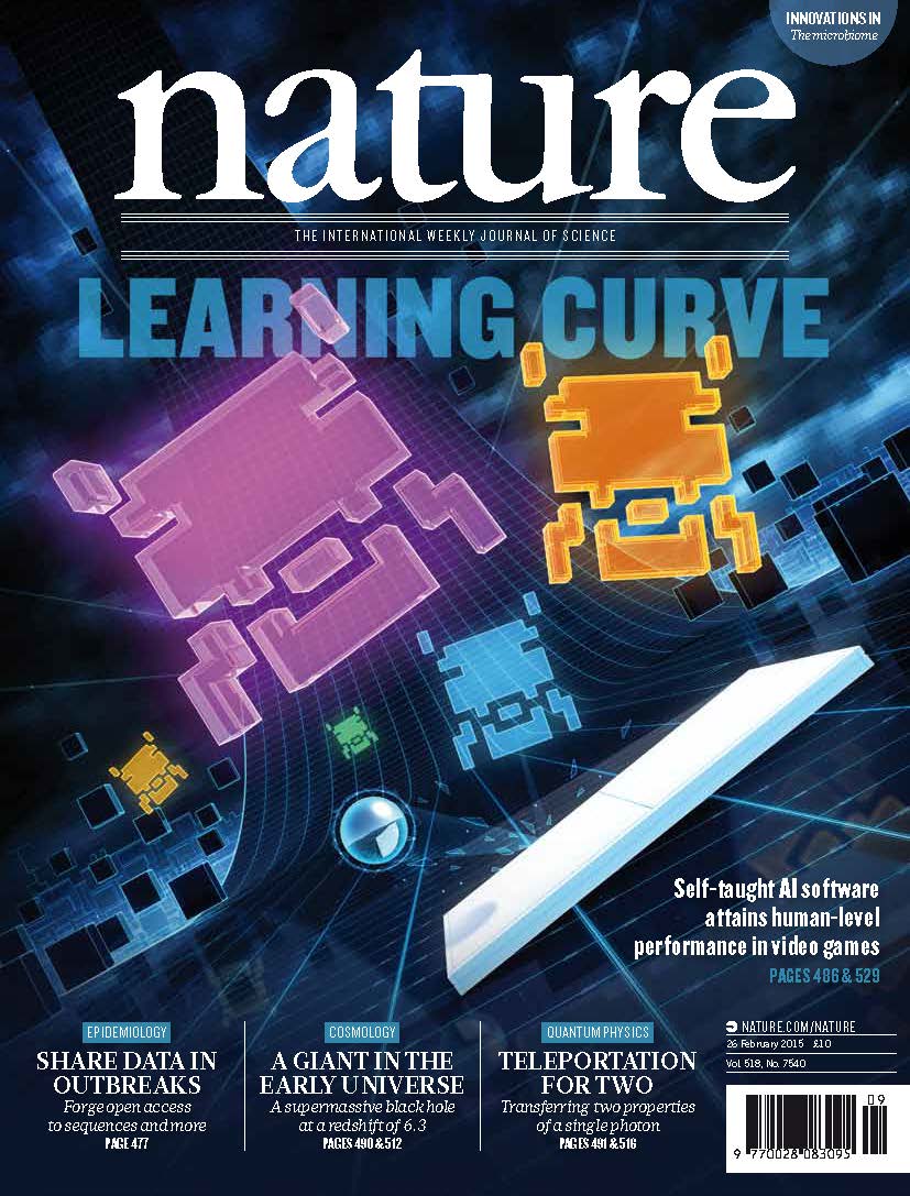
- If you want to learn more about this algorithm, you can read the original paper from DeepMind.
A gentle introduction to Reinforcement Learning
-
Case study: a simple game “Recycling is good”
-
The problem is as follows: you have an object that needs to be thrown away. You can either throw it in a normal bin or (better) throw it in a recycle bin. On the way to the recycle bin, there is a chocolate bar that you can eat, and you like chocolate!
- Problem statement:
- States: 5 states. 1 initial state (yellow cell) ; 2 normal states (gray) ; 2 terminal states (blue).
- Actions: 2 actions. You can either ‘go right’ or ‘go left’, you cannot stay idle.
- Initialization: you start in state 2.
- Termination: either you reach one of the terminal state or you move for 3 time steps.
-
Each action (cell change) takes you 1 time step. The time termination condition is to deter you from eating chocolate until the end of time!
- To match the problem goals, here is a way to define the rewards for this problem:
- Rewards: +1 if you reach state 4 (you are happy to eat chocolate) ; +2 if you reach state 1 (you throw your waste in the normal bin) ; +10 if you reach state 5 (better: you throw your waste in the recycle bin)
include images of the board + rewards from the course slides
How to evaluate a series of action?
- A straight-forward approach would just be to sum the rewards collected along the way. A more general approach is to compute the discounted return.
-
The discounted return \(R\) is the discounted sum of the rewards collected along the way (see formula below).
\[R = \sum \limits_{t=0}^{\infty } \gamma^t r_t = r_0 + \gamma r_1 + \gamma^2 r_2 + \cdots\]- where, \(0 \leq \gamma \leq 1\) is called the discount factor.
-
Why to we need to discount return? In real life, you are less confident about reaching long term goals. For example, a robot consumes some of its energy at each step. It is better for him to get rewards early than later when it may not have any energy left anymore.
-
The choice of the discount factor \(\gamma\) is an hyperparameter of your problem. Changing \(\gamma\) changes the optimal strategy.
- A strategy is defined by a policy. A policy is simply a function that tells you what action to take in a given state. Policy \(\pi : s -> a\). The policy that achieves the best return is called the optimal policy \($^\pi^*\).
What do we need to learn the optimal policy?
-
We define what is called a Q-table. The Q-table is a matrix where element \(Q^*(s,a)\) is the best return you can get if you take action \(a\) in state \(s\) and then act optimally.
-
If you know this Q-table, then the problem is solved. If you are in a given state \(s$, you can just take the action\)a\(that maximizes your return:\)\pi^(s) = a = \arg \max_{a’} Q^(s, a’)$$.
-
How to compute this Q-table? The corresponding optimal \(Q^*\) function must satisfy the Bellman equation:
\[Q^*(s,a) = r + \gamma \max_{a'} Q^*(s', a')\]- where, \(s'\) is the next state if you take action \(a'\) in state \(s\).
-
The table below is the optimal Q-table for our problem with a discount factor \(\gamma = 0.9\).
| state \ action | left | right |
| 1 | 0 | 0 |
| 2 | 2 | 9 |
| 3 | 8.1 | 10 |
| 4 | 9 | 10 |
| 5 | 0 | 0 |
- We can now compute the best policy by taking the argmax along the lines of the Q-table.
insert optimal policy image from slides
- Key takeaway
- This approach works well for our “toy” example. However we cannot solve the game of Go like this. Indeed in the game of Go the number of states is too big. We cannot store or work with a Q-table that big. In the next section, we will see how we can use Neural Network to approximate the Q-function. This is what we call Deep-RL.
Deep Q-Learning
- The main idea is to replace our Q-table with a Neural Network that learns a Q-function, which takes as input the id of the states defined as a one-hot vector and the output will be the Q-value for all possible actions.
- The question become how do we train such a network?
- Notice that this is a regression task. To train out network we might use the following loss,
- The problem is we don’t have the target value \($y\). To solve this we will use the Bellman equation at each iteration to approximate \($y\). The more our agent explores, the better our approximation of \($y\). Surprisingly, this process will converge. To see a proof of the convergence of Q-learning check out this paper by Franscisco Melo.
Applications of Deep Q-Learning
- Lets consider the classic game Breakout. You have a paddle controlled by the player and the goal is to break all the bricks with the ball without letting it pass by the paddle.
[insert Breakout game GIF]
-
How would you define the rewards? Whats the input of Q-network? And the output?
- The rewards will be positive for breaking bricks and winning and negative for loosing.
- The actions are (idle, left, right)
- The states will be a couple frames of the game.
-
We will define a CNN for our Q-network with the following architecture
[add architecture image]
-
Often we will need pre-processing of our states.
-
We will also need to define our initial and terminal states.
Training Tricks
- Experience replay - the problem with training one experience at a time, then an experience might only be seen once. Also, often the correct action will be the
- Experience reply instead holds experiences in an replay memory and then samples from the memory uniformly when training.
Exploration vs. Exploitation
- Using the \(\epsilon\) greedy action we will randomly choose actions with probability \(\epsilon\) and with probability \(1 - \epsilon\) we will use the action output by our Q-Network. We will often use a large \(\epsilon\) at the beginning of training and decay during training.
- Incorporating these tricks here is pseudo code for our.
- The same network has been applied to a variety of Atari games and has done very well.
Advanced Topics
- Tree Search
- Policy gradient methods - instead of learning a Q-value associated with a state and action, it learns directly the function that maps states to actions.
- Meta learning - If you have a distribution of tasks that look similar you don’t need to train from scratch.