CS230 • Deep Reinforcement Learning
- Motivation
- A Gentle Introduction to Reinforcement Learning
- Deep Q-Learning
- Applications of Deep Q-Learning
- Training Tricks in Deep Q-Learning
- Exploration vs. Exploitation
- Advanced Topics in Deep Reinforcement Learning
- Citation
Motivation
- Deep Reinforcement Learning (Deep-RL) lies at the intersection of two powerful paradigms: Reinforcement Learning (RL), which provides a framework for sequential decision-making under uncertainty, and Deep Learning (DL), which offers rich function approximation capabilities in high-dimensional spaces. Landmark achievements like AlphaGo and Deep Q-Networks helped propel Deep-RL into the spotlight—so let’s explore these breakthroughs in detail.
AlphaGo: A Breakthrough in Sequential Decision-Making
-
AlphaGo, developed by DeepMind, became the first program to defeat a world champion Go player, Lee Sedol, in 2016—an event that marked a milestone in AI history. Go had long been considered a particularly “AI-hard” domain.
-
The game’s complexity stems from its enormous state space and strategic depth:
- Played on a \(19 \times 19\) board.
- Each intersection may hold a black stone, a white stone, or be empty, yielding roughly \(3^{19\times19} \approx 10^{172}\) possible configurations.
- The branching factor and delayed rewards make this game intractable for conventional search-based systems.
-
The success of AlphaGo hinges on combining deep neural networks with intelligent search.
-
The following figure (source) illustrates AlphaGo’s two-network framework—policy network guiding move selection and value network evaluating board positions—coupled with Monte Carlo Tree Search (MCTS) to achieve master-level Go play:
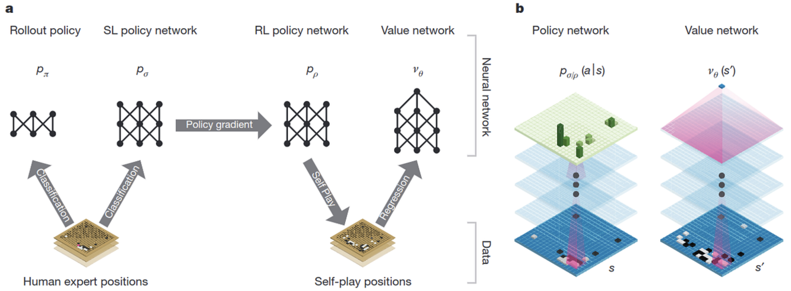
- AlphaGo initially used supervised learning to imitate strong human games, then improved through self-play using reinforcement learning to iterate on both networks.
Human-Level Control via Deep Reinforcement Learning
-
A year before AlphaGo’s breakthrough, DeepMind introduced the Deep Q-Network (DQN), which demonstrated super-human performance in numerous Atari 2600 video games—all from raw pixel input and without human-crafted features.
-
The DQN replaced the Q-table with a deep convolutional neural network—processing visual input, representing the state, and predicting Q-values for each action.
-
Here is a schematic of the DQN’s architecture, showcasing the convolutional layers processing game frames and the final outputs estimating action values:
-
The following figure (source) shows the CNN-based Deep Q-Network (DQN) architecture for Atari games, mapping stacked frames to Q-value outputs for each action.
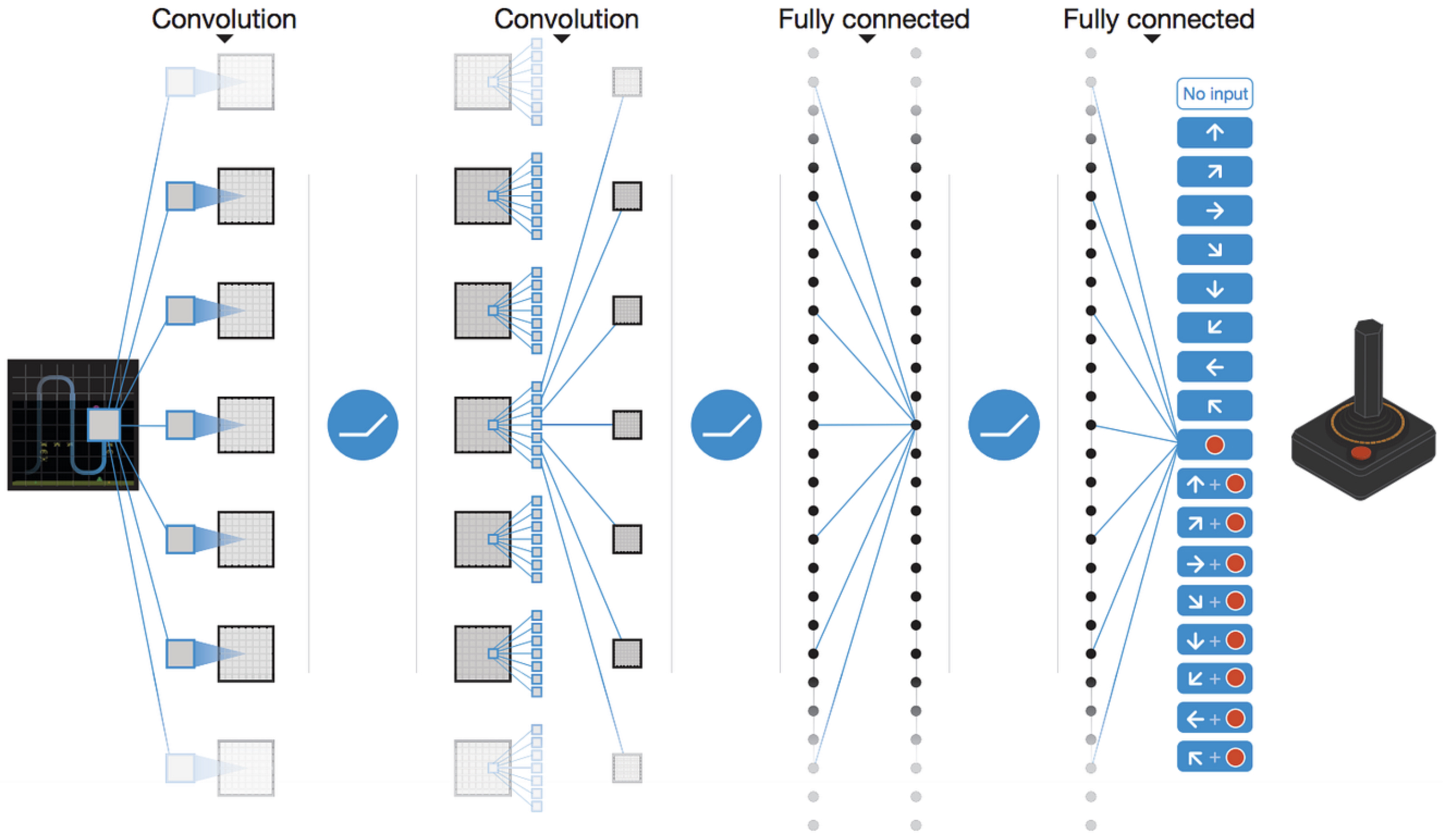
- This demonstrated that RL agents could learn directly from high-dimensional perceptual inputs—a key leap toward general-purpose learning agents.
Historical Context
- In 1997, IBM’s Deep Blue defeated Garry Kasparov at chess using brute-force search with engineered evaluation heuristics.
- In 2015, DeepMind’s DQN mastered diverse Atari games with a single general-purpose algorithm.
-
In 2016, AlphaGo defeated a world-class Go player using a hybrid of deep neural networks and tree search.
- The more than 18-year gap between Deep Blue and AlphaGo reflects the significantly higher complexity of Go and the necessity of function approximation via deep learning to scale to such domains.
Key Insights
- RL reframes problems from predicting immediate labels to optimizing sequences of actions toward long-term goals.
- Deep neural networks provide scalable function approximation to represent value functions and policies in complex, sensory-rich environments.
- The synergy of RL and DL enabled agents capable of learning from raw perceptual data—without hand-crafted features or game-specific logic.
A Gentle Introduction to Reinforcement Learning
- To build an intuitive foundation in Reinforcement Learning (RL), we explore a toy example that embodies its core concepts: states, actions, rewards, policies, and optimality. This simple game illustrates how agents evaluate action sequences and learn to make optimal decisions.
Case Study: “Recycling Is Good”
-
Imagine a small grid world where your goal is to dispose of waste:
- You can choose between a normal bin (less desirable) and a recycling bin (more desirable).
- On the path lies a chocolate bar, tempting but sub-optimal in the long run.
-
Environment Setup:
-
States: 5 states total:
- 1 initial state (yellow cell),
- 2 intermediate non-terminal states (gray cells),
- 2 terminal states (blue cells).
- Actions: You can go “left” or “right”; no idle action.
- Start: Always in state 2.
- Termination: Reaching a terminal state or after 3 moves.
-
-
Rewards:
- +1 for chocolate (state 4),
- +2 for normal bin (state 1),
- +10 for recycling bin (state 5).
-
This payoff structure encourages reaching the recycling bin despite chocolate’s lure.
-
This visualization highlights how choices in the middle states cascade into different terminal outcomes, each with its own return.
Evaluating Action Sequences
-
Rather than merely summing rewards, RL employs the concept of discounted return:
\[R = \sum_{t=0}^{\infty} \gamma^t r_t = r_0 + \gamma r_1 + \gamma^2 r_2 + \cdots\]- where:
- \(r_t\): reward at time step \(t\).
- \(\gamma\): discount factor ( \(0 \leq \gamma \leq 1\) ).
- where:
-
A low \(\gamma\) prioritizes immediate rewards, while a high \(\gamma\) values long-term returns. This balances risk and future uncertainty.
Policies and Optimality
- A policy \(\pi\) maps each state to an action:
-
The goal is the optimal policy \(\pi^*\), maximizing expected return in each state:
\[\pi^*(s) = \arg\max_a Q^*(s, a)\]- where \(Q^*(s, a)\) is the maximum achievable return from state \(s\), taking action \(a\), and acting optimally thereafter.
The Q-Function & Bellman Equation
-
The optimal Q-function satisfies the recursive Bellman Optimality Equation:
\[Q^*(s, a) = r + \gamma \max_{a'} Q^*(s', a')\]- where, \(s'\) is the next state reached by taking action \(a\) from \(s\). This equation formalizes how current decisions hinge on future best decisions.
Example: Optimal Q-Table
- For our example with \(\gamma = 0.9\), the optimal Q-values are:
| State / Action | Left | Right |
|---|---|---|
| 1 | 0 | 0 |
| 2 | 2 | 9 |
| 3 | 8.1 | 10 |
| 4 | 9 | 10 |
| 5 | 0 | 0 |
- Selecting the highest Q-value per state yields the optimal policy.
Key Takeaway
- This tabular approach works for small, discrete puzzles, but does not scale to complex domains like Go or visual games. Here, the state space is astronomic, and direct Q-table methods fail. This necessity motivates Deep Reinforcement Learning, where neural networks approximate the Q-function rather than attempting to enumerate it.
Deep Q-Learning
-
The limitations of tabular Q-learning—namely, its inability to scale to large or visually rich domains—motivated the transition to function approximation via neural networks. In Deep Q-Learning (DQN), we replace the Q-table with a neural network that outputs action-value estimates for each state-action pair:
\[Q(s, a; \theta) \approx Q^*(s, a),\]- where \(\theta\) are the parameters of the network. This formulation enables agents to learn from high-dimensional inputs like raw images, paving the way for applications in robotics, gaming, and more.
-
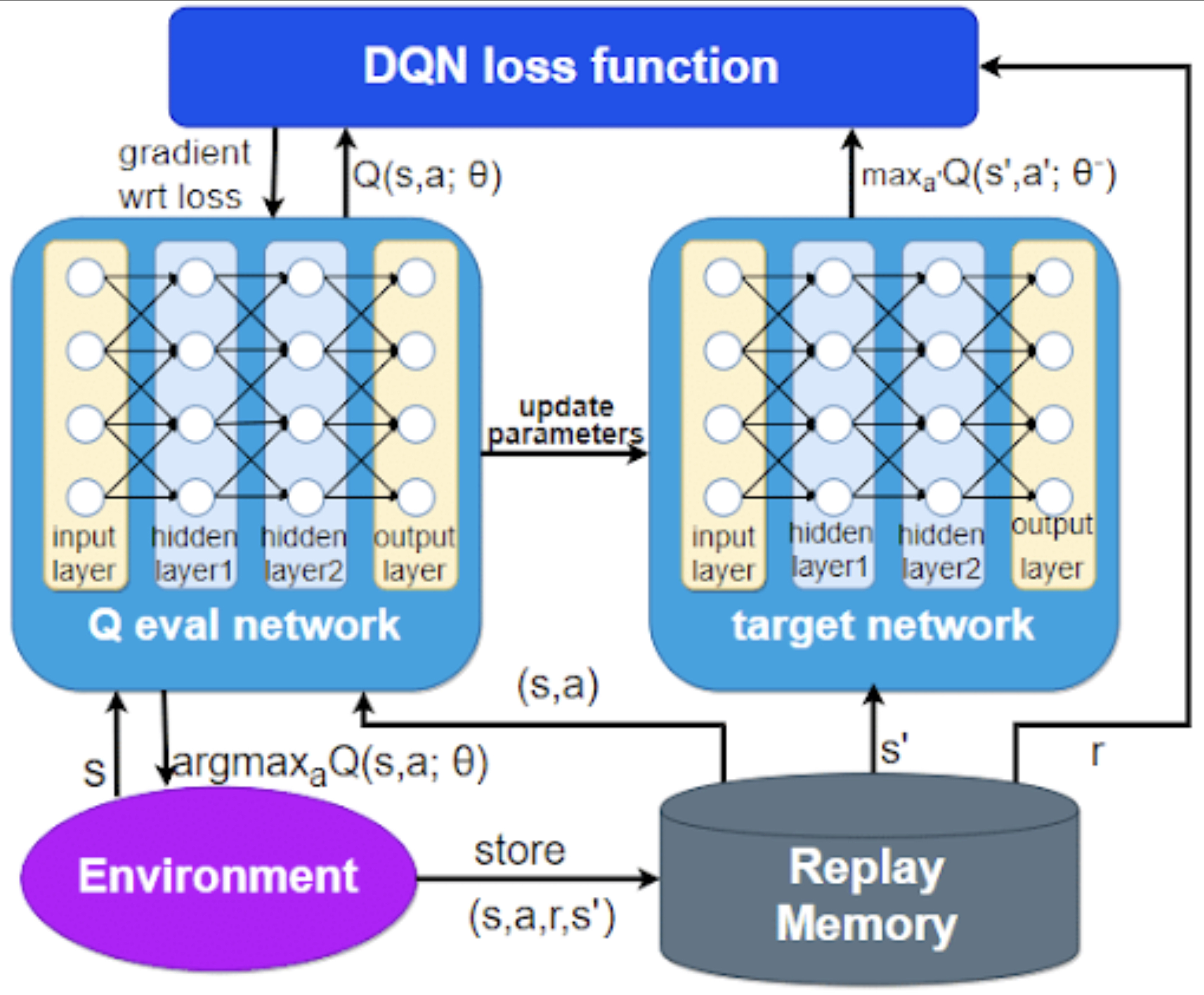
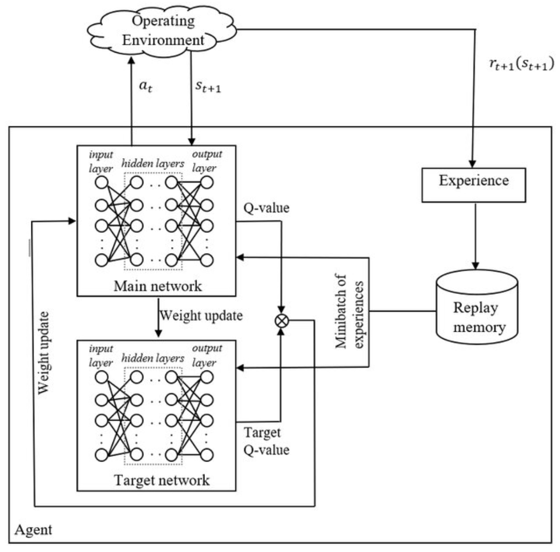
The following figure illustrates the architecture of the DQN framework, highlighting the evaluation network, target network, and the replay memory used for stabilization. Specifically, it illustrates how the evaluation (online) network and target network interact via replay memory to stabilize Deep Q-Learning training.
-
In this schematic:
- The evaluation network computes \(Q(s, a; \theta)\), producing Q-value estimates used to select actions.
- Recent transitions \((s, a, r, s')\) are stored in a replay memory buffer.
- The target network, with parameters \(\theta^{-}\), provides stable targets \(y = r + \gamma \max_{a'} Q(s', a'; \theta^{-})\) for training.
- Through these components, the DQN algorithm minimizes the loss \(L(\theta) = \left(y - Q(s, a; \theta)\right)^2\) by sampling mini-batches from replay memory—a key mechanism for reducing correlation in training data and improving convergence.
Neural Approximation of the Q-Function
- In practice, the DQN takes a state \(s\) as input—such as a stack of video game frames—and outputs a vector of Q-values, each corresponding to a possible action. The implied policy is:
- This renders the agent capable of making decisions based on rich sensor data or visual input, without hand-designed features.
Training the Q-Network
-
Training the Q-network is formulated as a regression task:
\[L(\theta) = \big(y - Q(s, a; \theta)\big)^2,\]- where the target
- is derived via bootstrapping from the Bellman equation. Leveraging a separate target network (\(\theta^{-}\)) that updates more slowly ensures training remains stable and avoids oscillations.
Why This Approach Works
- Despite relying on predictions to update other predictions, Q-learning with nonlinear function approximation converges empirically when stabilized properly. Experience replay decouples samples, and target networks dampen oscillations—together enabling deep networks to approximate optimal Q-functions in challenging environments.
Key Insights
- Replacing a Q-table with a neural network enables scaling to continuous or high-dimensional state spaces.
- Experience replay and target networks are essential stabilizing mechanisms.
-
The overall DQN framework allowed breakthroughs like Atari game mastering and later more complex applications.
- The following figure shows an agent playing Atari Breakout—using a DQN, the agent controls the paddle to bounce the ball and break bricks—visualizing how the network interacts with the environment in real-time.
Applications of Deep Q-Learning
- The landmark demonstration of Deep Q-Learning’s potential can be seen in how it learned to play Atari 2600 games—most notably, Breakout—directly from raw pixel input. This established the feasibility of combining perception and decision-making in a single end-to-end learning framework.
Case Study: Breakout
-
Breakout is a classic arcade game in which:
- The agent controls a paddle at the bottom of the screen.
- A ball bounces off the paddle to break bricks at the top.
- The game ends when the ball passes below the paddle.
RL Formulation for Breakout
- States: Raw pixel frames from the game. Typically, four consecutive frames are stacked to capture motion.
- Actions: A discrete action space, usually {idle, left, right}.
-
Rewards:
- Positive for breaking a brick.
- Positive for clearing all bricks (winning).
- Negative for losing (letting the ball fall).
Training on Pixel Input
- The DQN directly takes pixel-based state representations without manual feature engineering, relying on the network’s convolutional layers to learn useful representations of the environment.
- This approach was revolutionary. DeepMind demonstrated that a single algorithm could master multiple games—learning from high-dimensional inputs using stable RL training techniques such as experience replay and target networks.
Strategic Play and Emergent Behavior
-
One of the most striking outcomes was the DQN agent discovering sophisticated strategies—particularly tunneling, wherein the agent creates a gap on the side of bricks and funnels the ball to the top—an emergent behavior seldom seen in human play.
-
This capability underscores the potential for end-to-end RL agents to surpass human intuition using only reward signals and raw sensory input.
Significance and Legacy
- Demonstrated general-purpose learning from raw pixels with no explicit game knowledge.
- Validated that a unified architecture (CNN + Q-learning) could master diverse decision-making tasks.
- Highlighted the importance of stabilization techniques (experience replay, target networks) in enabling deep RL agents to learn from high-dimensional, non-stationary data.
- This application laid the foundation for a broader wave of research in Deep RL across domains like robotics, autonomous control, and language-guided agents.
Training Tricks in Deep Q-Learning
-
While the deep approximation of Q-values is powerful, combining function approximation with bootstrapping introduces instability. To address this, Deep Q-Learning incorporates essential stabilizing techniques: experience replay, target networks, reward clipping, and frame skipping.
-
The following figure (source) illustrates how the evaluation (online) network, target network, and replay memory work together to stabilize training in Deep Q-Learning. Specifically. the diagram shows the interaction among the online Q-network, the target network, and the experience replay buffer during training, showing how transitions are sampled and target values are computed.
Experience Replay
-
When the agent interacts with its environment, consecutive experiences are highly correlated—a problematic scenario for neural network training, which assumes i.i.d. samples. Experience replay addresses this by:
- Storing transitions \((s, a, r, s')\) in a replay buffer as they occur.
-
Sampling mini-batches randomly from this buffer during training, which:
- Breaks the temporal correlations.
- Enhances data efficiency by reusing past experiences multiple times.
- Helps prevent catastrophic forgetting and improves generalization.
Target Networks
-
Using the same network to generate both current value estimates and target Q-values leads to instability:
\[y = r + \gamma \max_{a'} Q(s', a'; \theta),\]- updates can continually shift the target, causing divergence.
-
By introducing a target network—a periodically updated copy of the main Q-network—the algorithm stabilizes its learning targets. The target network’s parameters \(\theta^{-}\) remain fixed for several updates before being synchronized with the main network.
-
This stabilizes training, reducing oscillations and divergence caused by chasing a moving target.
Reward Clipping
-
Large reward magnitudes can induce high variance in updates. Deep Q-Learning often clips rewards to a small fixed range (commonly \(\{-1, 0, +1\}\)):
- Preserves the signal of reward’s sign.
- Prevents outlier rewards from destabilizing learning.
-
This simple heuristic was particularly effective in the Atari experiments but is applied based on task-specific considerations.
Frame Skipping
-
Processing every frame in visual environments like Atari is both computationally expensive and often unnecessary:
- The agent applies each chosen action for multiple consecutive frames (e.g., 4),
- Reduces input redundancy,
- Speeds up training while preserving essential dynamics.
Benefits
-
These techniques collectively enable deep RL to operate reliably in complex, high-dimensional environments:
- Experience replay ensures sample efficiency and breaks input correlation.
- Target networks stabilize training by decoupling learning targets.
- Reward clipping controls update variance.
- Frame skipping accelerates learning while capturing key dynamics.
-
Together, they transformed Q-Learning from a fragile algorithm into a robust framework capable of learning from raw sensory inputs across diverse domains.
Exploration vs. Exploitation
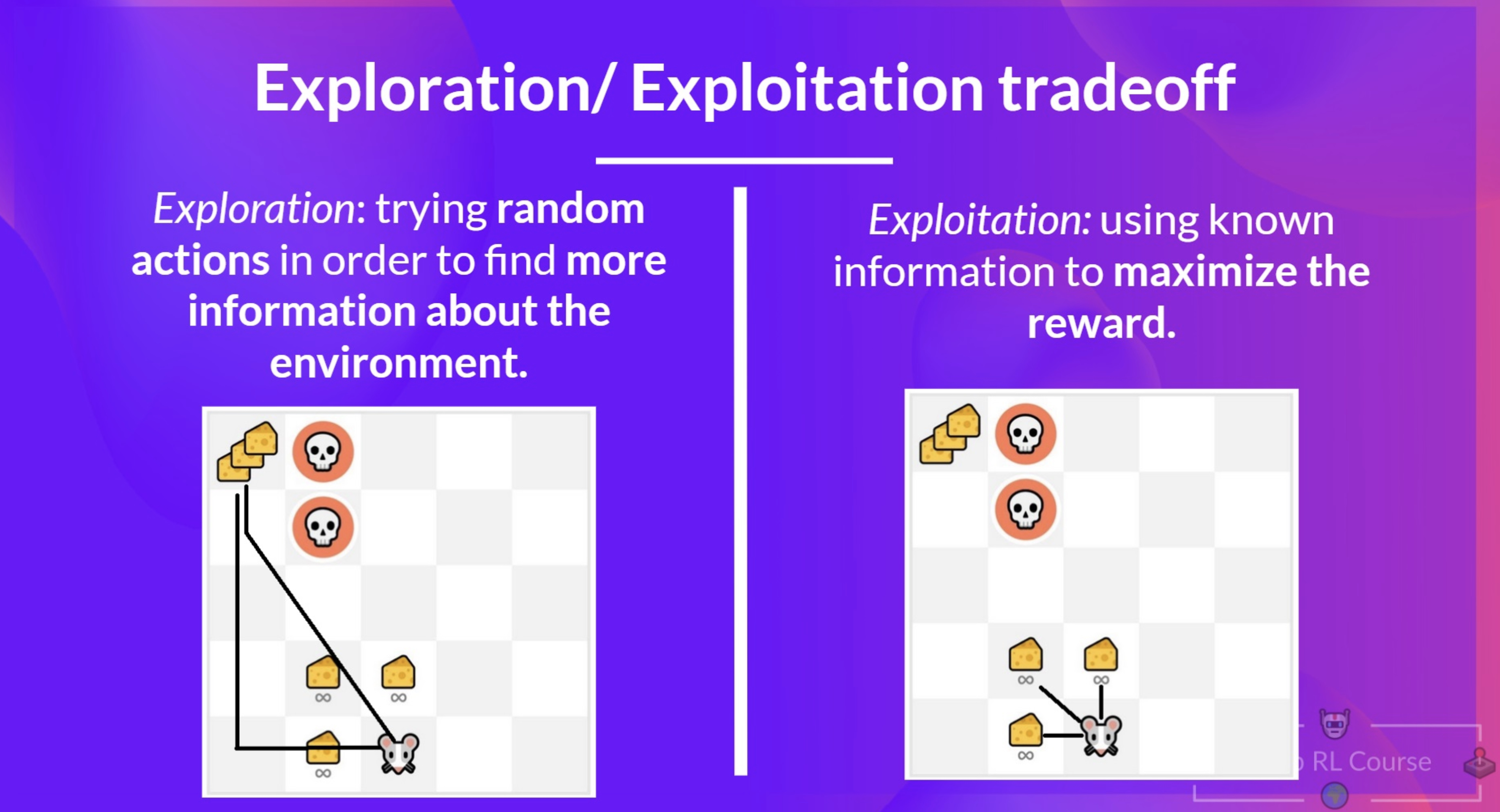
- In reinforcement learning, agents face a core dilemma: they must explore new actions to discover potentially better strategies, while also exploiting what they already know to maximize reward. This tension is at the heart of the design of effective RL algorithms.
The Epsilon-Greedy Strategy
-
A widely used method to strike this balance is the epsilon-greedy policy:
- With probability \(\epsilon\), the agent explores—choosing a random action.
- With probability 1–\(\epsilon\), it exploits—choosing the action that currently maximizes the estimated Q-value:
-
This simple yet powerful mechanism ensures the agent does not get stuck prematurely on suboptimal behavior.
-
The following figure (source) illustrates the exploration vs. exploitation trade-off: during the exploration phase, the agent explores by selecting a random action, while during the exploitation phase, it exploits its current knowledge by choosing the action with the highest estimated value.
Decay of Epsilon Over Time
-
Dynamic adjustment of \(\epsilon\) is essential for performance:
- Start with a high \(\epsilon\) (e.g., near 1) to encourage broad exploration.
- Gradually decay \(\epsilon\) toward a low value (e.g., 0.1 or 0.01) as the agent learns more.
-
This schedule transitions the agent from exploration to exploitation in a controlled manner.
-
In practice, epsilon decay can follow linear or exponential schedules—and choosing the decay rate is critical to convergence and sample efficiency.
Why Use Epsilon-Greedy?
-
Epsilon-greedy remains popular in Deep Q-Learning for several reasons:
- Simplicity: Easy to implement and understand.
- Control: Direct parameter \(\epsilon\) offers an intuitive way to adjust exploration.
- Stability: Offers clearer behavior across different environments compared to alternatives.
-
Although other strategies like softmax (Boltzmann) selection or UCB can offer more efficient exploration, they often require tuning and may lack the robustness and simplicity of epsilon-greedy, especially across disparate environments.
Advanced Variants and Considerations
-
Several refinements enhance epsilon-greedy’s effectiveness:
- Epsilon Decay Schedules: Linear or exponential decay based on training steps or episodes.
- Adaptive Epsilon: Allow \(\epsilon\) to decrease based on learning progress or performance thresholds.
- Optimistic Initialization: Initialize value estimates to high values to encourage exploration.
- Contextual Variants: Vary \(\epsilon\) based on the state or context—explore more in uncertain regions of the state space.
Comparative Analysis
| Strategy | Exploration Behavior | Advantage |
|---|---|---|
| Epsilon-Greedy | Random action with probability \(\epsilon\), otherwise greedy | Simple, stable, widely applicable |
| Softmax / Boltzmann | Probabilistic action selection based on Q-values | Smooth exploration, but sensitive to temp |
| UCB / Bonus Methods | Adds uncertainty bonus to favor less-visited states | Data-efficient, more complex to tune |
Key Insight
- The exploration–exploitation trade-off is fundamental: without enough exploration, an agent may remain stuck in poor strategies; with too much exploration, it never consolidates learning. Epsilon-greedy offers a flexible yet tractable means to navigate this trade-off—transitioning gradually from curiosity toward competence.
Advanced Topics in Deep Reinforcement Learning
- Beyond Deep Q-Learning, the field of Deep Reinforcement Learning (Deep-RL) has expanded into a variety of powerful approaches. These methods address challenges such as planning, continuous actions, data efficiency, and generalization capabilities. Below, we explore several key directions.
Tree Search with MCTS (Monte Carlo Tree Search)
-
Tree search methods—particularly Monte Carlo Tree Search (MCTS)—enable forward-planning through simulated exploration of future action sequences. This is instrumental in domains like Go, where long-term strategy is vital.
-
The following figure illustrates the four core phases of MCTS as used in AlphaGo’s search algorithm: selection, expansion, simulation, and backup. In other words, the MCTS process involves selecting promising nodes, expanding leaf nodes, simulating to estimate outcomes, and backing up value estimates to guide future search. It also highlights how neural networks inform both the search (via policy priors) and evaluation (via value estimates).
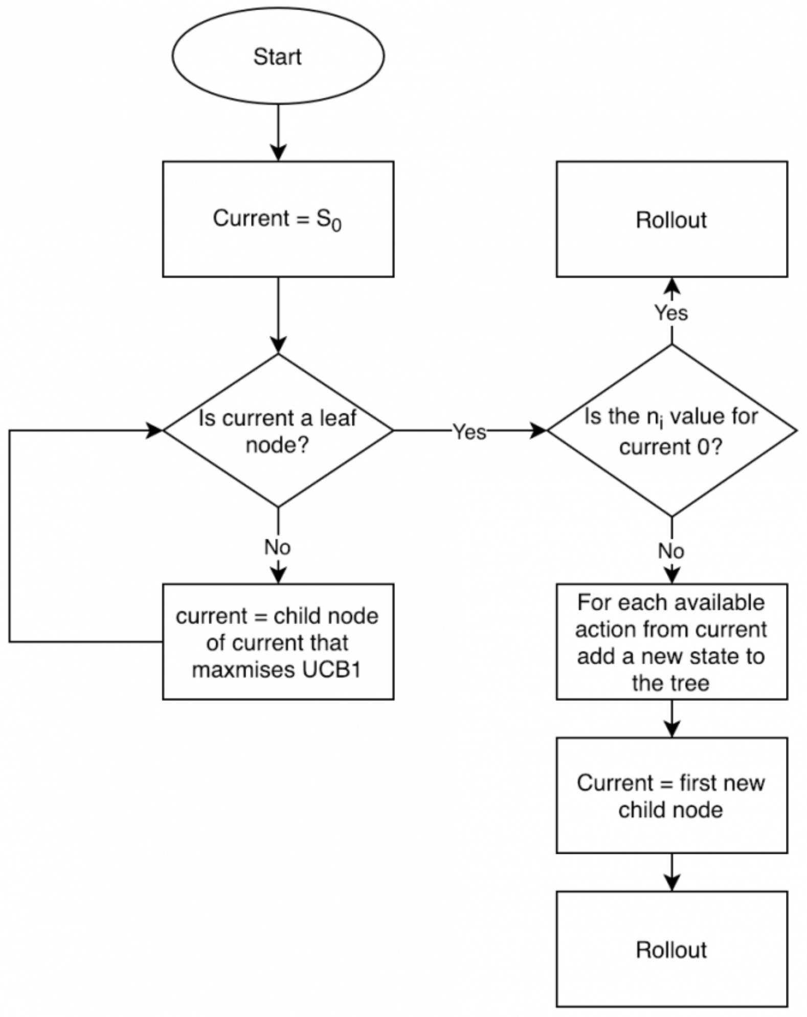
- AlphaGo combined MCTS with multiple neural networks—including supervised policy, rollout policy, RL policy, and a value network—to drive search and evaluation. These components were trained using expert games and self-play, bootstrapped by policy gradients and supervised learning.
Policy Gradient Methods & Actor–Critic
- Instead of approximating value functions, policy gradient methods directly optimize the policy \(\pi_\theta(a \| s)\). These are particularly effective for high-dimensional or continuous action spaces.
Policy Gradients
- These methods estimate gradients of policy parameters that maximize expected return:
- This treats policy as the primary object of learning. Techniques like REINFORCE fall into this category ([Lil’Log][4], [Medium][5]).
Actor–Critic Algorithms
- These combine a policy network (actor) with a value estimator (critic). The actor proposes actions, while the critic evaluates them using value information to reduce variance and improve training efficiency.
Modern Policy Optimization: PPO
-
Proximal Policy Optimization (PPO) is a contemporary policy gradient approach that stabilizes updates via clipped probability ratios, achieving high performance without complex constraints like those in TRPO.
-
The following figure visualizes the interaction between actor and critic networks by illustrating the DDPG actor-critic framework, where the actor defines the policy, and the critic evaluates actions via Q-learning. Both networks have online and target variants to stabilize training.
| 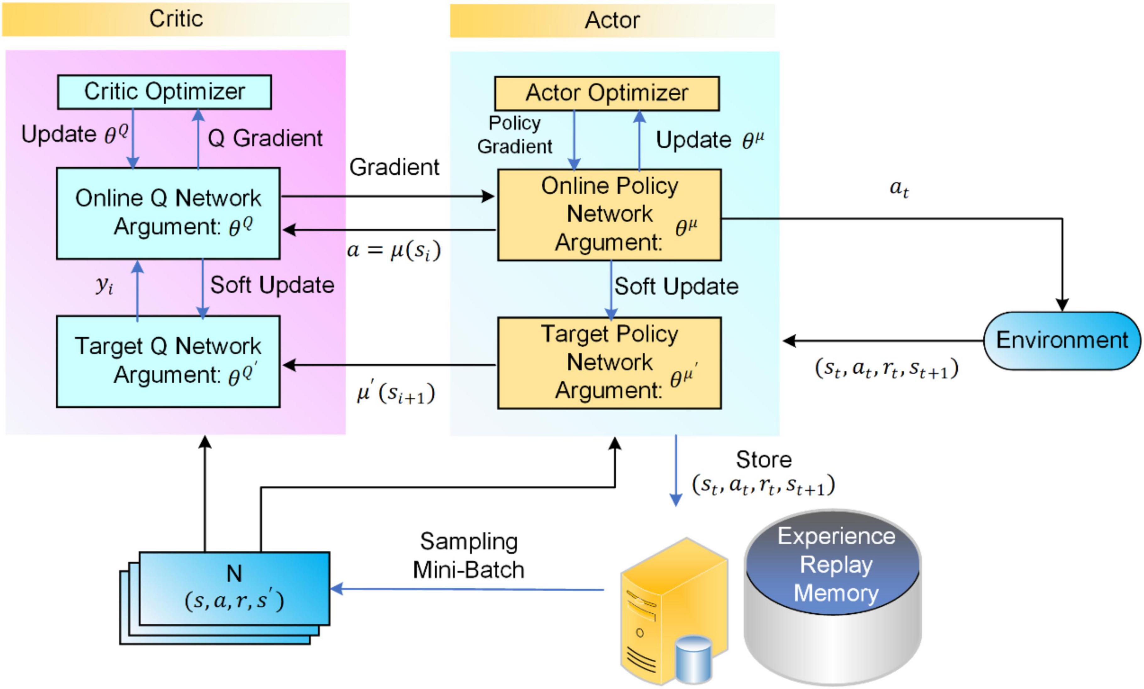 |
Meta-Learning & Beyond
-
To enable agents that learn to learn, meta-learning enables rapid adaptation across related tasks.
- Meta-Learning: Learns priors that allow quick adaptation to new environments (e.g., MAML).
- Model-Based RL: Learns an internal model of dynamics for planning and improved sample efficiency.
- Hierarchical RL: Decomposes tasks into reusable sub-policies or skills for structured, long-horizon behavior.
- Multi-Agent RL: Manages interactions between multiple learning agents—cooperative, competitive, or mixed.
-
Offline / Batch RL: Learns from static datasets without active exploration—critical in domains where interaction is limited or risky (healthcare, autonomous driving).
- These areas push Deep-RL toward more general, efficient, and robust agent behavior.
Summary & Future Directions
- MCTS enriches RL with explicit planning and search, as seen in AlphaGo.
- Policy-gradient and actor–critic methods allow direct optimization of policies, handling complex and continuous tasks.
- Advanced techniques such as PPO improve stability and reliability of training.
-
Expanding frontiers in meta-learning, hierarchy, and multi-agent settings aim to imbue agents with broader intelligence and adaptability.
- Together, these advanced methods reflect the dynamism of the field—moving beyond game-playing benchmarks toward scalable, transferable intelligence.
Citation
If you found our work useful, please cite it as:
@article{Chadha2020DeepRL,
  title   = {Deep Reinforcement Learning},
  author  = {Chadha, Aman},
  journal = {Distilled Notes for Stanford CS230: Deep Learning},
  year    = {2020},
  note    = {\url{https://aman.ai}}
}