CS230 • Convolutional Neural Networks

• Overview
  • Core principles of CNNs
  • Motivation for CNN layers
• Edge detection
  • Why do filters detect edges?
  • Practical considerations
  • Mathematical summary
  • Connections to learning
  • Takeaways
• Padding
  • Output sizing with padding and stride
  • Why padding matters in deep nets
  • Choices of boundary handling
  • Connection to gradient flow
  • Practical notes
• Strided Convolutions
  • Mathematical formulation
  • Interpretation
  • Constraints and valid filters
  • Worked example
  • Connections to modern architectures
• Cross-Correlation vs. Convolution
  • Classical convolution
  • Cross-correlation
  • Implications
  • Practical takeaway
• Convolutions over Volume
  • Convolution with channels
  • Multiple filters and feature maps
  • Interpretation
  • Computational cost
• One-Layer Convolutional Network
  • Linear activation (pre-activation stage)
  • Non-linear activation (post-activation stage)
  • Dimensions recap
  • Parameter count
  • Intuition
• Pooling Layers
  • Mechanics of pooling
  • Intuition
  • 3D pooling (multi-channel inputs)
  • Advantages of pooling
  • Modern perspective
• Why We Use Convolutions
  • Fully connected baseline
  • Convolutional alternative
  • Two key ideas
  • Implications
• Classic Networks
  • LeNet-5
  • AlexNet
  • VGG-16
  • ResNet
  • 1×1 Convolution
  • Inception Network (GoogLeNet)
  • Summary of classic networks
• Competitions and Benchmarks
  • Benchmark-driven progress
  • Test-time strategies
  • Practical considerations
• Citation

Overview

• Neural networks applied directly to flattened image data face a major scalability problem. A modestly sized color image of resolution \(1000 \times 1000 \times 3\) contains 3 million input features. Feeding such a vector into a fully connected layer would require tens of millions of parameters, resulting in computational intractability and a severe risk of overfitting, since the model capacity would vastly exceed the amount of training data.

• Convolutional neural networks (CNNs) overcome these limitations by exploiting the inherent structure of natural images. Instead of treating every pixel as independent, CNNs leverage two key properties:

  1. Local spatial correlation

     • Neighboring pixels are highly correlated and jointly define meaningful structures such as edges, corners, or small textures.
     • By restricting connections to small neighborhoods, CNNs efficiently capture these local patterns without wasting capacity on irrelevant long-range connections.

  2. Translation invariance

     • Objects can appear anywhere in an image, but their local features remain the same.
     • CNNs achieve this by parameter sharing: the same filter is applied across all spatial positions. This ensures that once a feature detector (e.g., an edge detector) is learned, it can detect the feature regardless of location.

Core principles of CNNs

• CNNs rest on three foundational principles that distinguish them from fully connected architectures:

  • Sparse connectivity: Each neuron connects only to a small local region of the input (the receptive field), unlike in fully connected layers where each neuron sees the entire input.
  • Parameter sharing: A single set of filter weights is reused across all positions, drastically reducing the total number of parameters.
  • Hierarchical feature learning: By stacking multiple convolutional and pooling layers, CNNs build representations that grow in abstraction — from simple edges, to textures, to object parts, and eventually to whole objects.

Motivation for CNN layers

• CNNs achieve their power by combining a small set of specialized layer types, each contributing a distinct role in the feature extraction process:

  • Convolutional layers learn filters that detect local features such as edges, corners, and textures.
  • Activation functions (e.g., ReLU) inject nonlinearity, enabling the network to approximate complex mappings.
  • Pooling layers downsample feature maps, reducing spatial size and providing invariance to small translations.
  • Fully connected layers (usually near the output) combine abstract features into final predictions for classification or regression.

• This modular design, guided by locality, sharing, and hierarchy, allows CNNs to achieve state-of-the-art results in tasks ranging from image classification and object detection to semantic segmentation and self-supervised representation learning.

Edge detection

• Edge detection is a foundational operation in both classical image processing and modern convolutional neural networks (CNNs). Intuitively, edges correspond to spatial locations where the image intensity varies rapidly; mathematically, these are regions where spatial derivatives of the image are large in magnitude. Detecting such structure is useful because edges delineate object boundaries, reveal texture, and provide robust, low-level cues that downstream models can exploit.

• From a signal-processing viewpoint, an image is a discrete function \(I:\mathbb{Z}^2 \to \mathbb{R}\) (grayscale) or \(\mathbb{R}^3\) (RGB). A linear, shift-invariant operator on images can be implemented by a discrete convolution with a small filter (kernel) \(K\in\mathbb{R}^{f\times f}\). For a 2D image and a single filter, the valid discrete convolution at location \((i,j)\) is

  \[(S = I \ast K)\,(i,j) \;=\; \sum_{u=0}^{f-1}\sum_{v=0}^{f-1} I(i+u,\,j+v)\,K(u,v),\]
  • where we use the computer-vision convention (no kernel flip), so this is strictly cross-correlation; classical convolution flips \(K\) both horizontally and vertically. In practice, the distinction is immaterial for learning because filters are learned jointly with the sign/orientation convention; nonetheless, it is good to be precise. With an input of spatial size \(n_h\times n_w\) and a square filter of size \(f\times f\), the spatial size of the valid output is \((n_h-f+1)\times (n_w-f+1)\).

Why do filters detect edges?

• If we approximate spatial derivatives by finite differences, then small, signed filters that compute differences between neighboring pixels produce large responses on intensity transitions and near-zero responses in flat regions. Classical, hand-crafted derivative filters such as Prewitt, Sobel, and Scharr implement this idea and differ chiefly in how they weight central versus peripheral pixels to trade off noise suppression for localization Prewitt (1970), Sobel and Feldman (1968), Scharr (2000). The discrete gradient components are commonly realized as:

  \[G_x = I \ast K_x,\qquad G_y = I \ast K_y,\]
  • and combined into magnitude and orientation,
  \[\|\nabla I\|_2 = \sqrt{G_x^2 + G_y^2},\qquad \theta = \arctan2(G_y,\,G_x),\]
  • which summarize edge strength and direction.

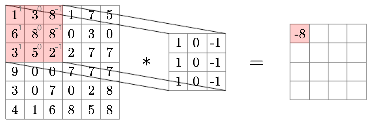
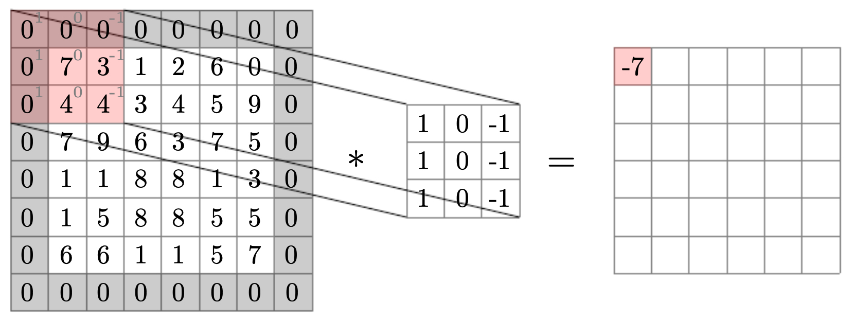
• The following figure introduces the local computation performed by a 2D filter: a sliding, elementwise product between the filter coefficients and the underlying image patch, followed by a sum. In other words, a convolution over a matrix is the element-wise product between a filter and a same-sized subpatch of the matrix, accumulated to a single scalar. The value computed over the upper-left patch becomes the upper-left entry of the output response map. Reading the diagram left-to-right helps connect three ideas at once: alignment of the receptive field, the multiply–accumulate at a single location, and the tiling of such computations to populate the entire output.

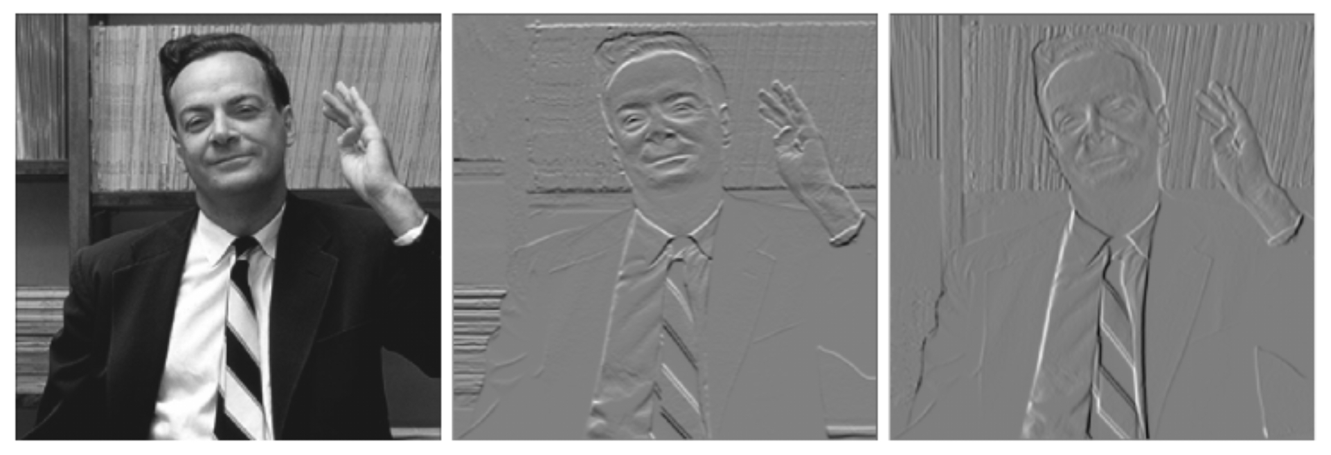
• The following figure illustrates the qualitative effect of applying horizontal (middle) and vertical (right) edge filters to a natural image (left). Dark pixels indicate strong positive responses (edges aligned with the filter’s preferred orientation), white pixels indicate strong negative responses (edges with opposite orientation), and mid-gray indicates weak or no detected edge. In practice, one may combine oriented responses using \(\sqrt{G_x^2+G_y^2}\) to obtain an orientation-agnostic strength map, then thin and threshold responses (e.g., non-maximum suppression and hysteresis as in the Canny detector (Canny (1986)). As you examine the trio, notice how vertical structures (e.g., facades, tree trunks) dominate the vertical filter output, while horizons and rooftops light up in the horizontal filter output.

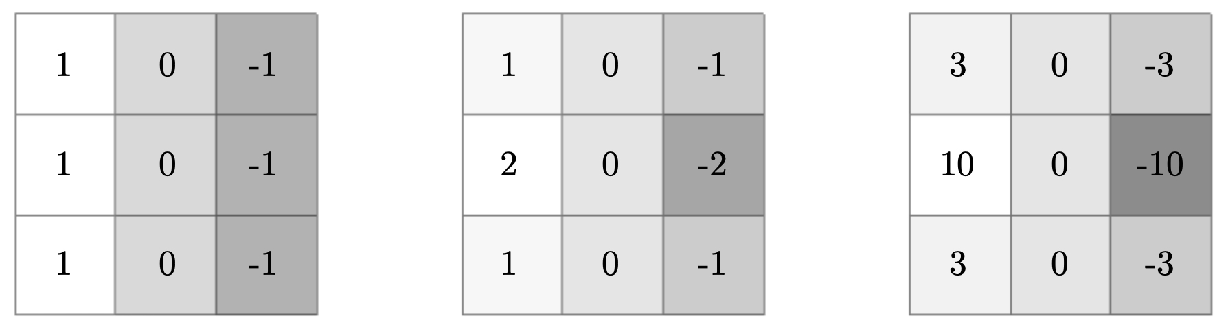
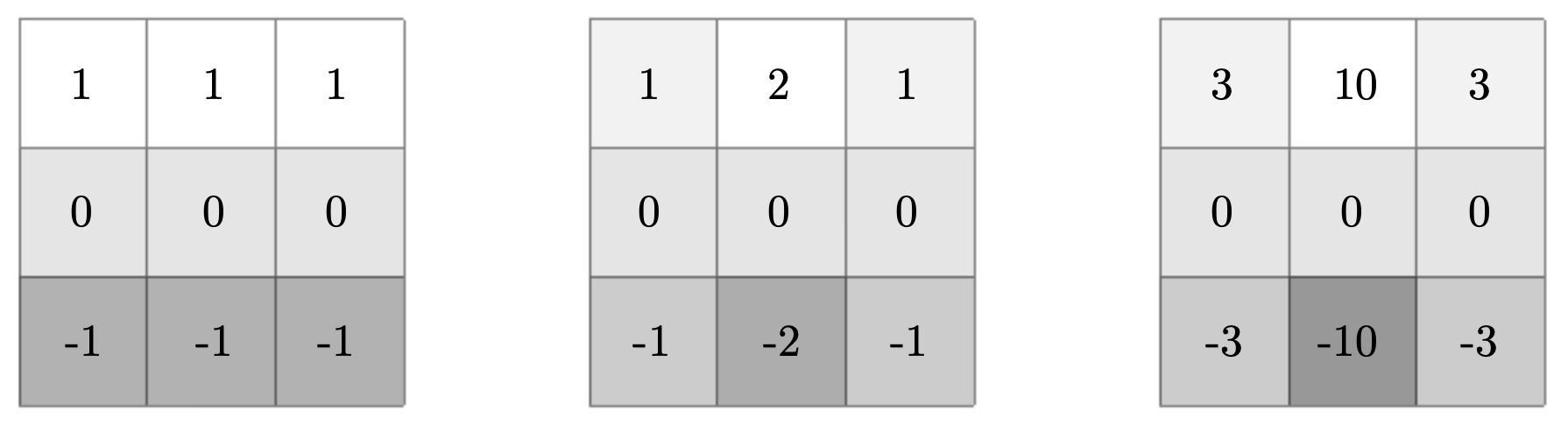
• The following figures catalog common vertical and horizontal edge-detection filters. The top panel presents vertical kernels—standard difference, Sobel, and Scharr—each implementing a distinct compromise between derivative accuracy and smoothing. The bottom panel shows their horizontal counterparts obtained by transposition (or rotation). Observe how Sobel’s heavier center weights add robustness to noise, while Scharr’s carefully chosen coefficients improve rotational symmetry, yielding more isotropic gradient estimates—beneficial when edge orientations vary continuously in natural scenes.

Practical considerations

1. Normalization and dynamic range. Because convolution outputs are sums of products, their magnitudes can vary widely. It is common to normalize responses (e.g., rescale to \([0,1]\) or standardize per feature map) or to place normalization layers (BatchNorm/InstanceNorm) after learned convolutions to stabilize optimization.

2. Orientation coverage. A single vertical (or horizontal) derivative kernel responds strongly to edges with that orientation. To capture edges at arbitrary orientations, one can deploy a bank of oriented filters (e.g., rotated Sobel/Scharr), or compute \((G_x,G_y)\) and derive \(\|\nabla I\|\) and \(\theta\).

3. Nonlinearity and thresholding. Classical pipelines thin edges via non-maximum suppression along \(\theta\) and use hysteresis thresholds to maintain connectivity (as in Canny (1986)). In CNNs, learned nonlinearities (ReLU, GELU) and subsequent layers typically replace hand-crafted post-processing by learning task-specific invariances.

4. From fixed to learned filters. Although CNNs learn filters end-to-end, it is a recurring observation that the first layer often resembles oriented band-pass (Gabor-like) derivatives LeCun et al. (1998), Krizhevsky et al. (2012), Simonyan and Zisserman (2015). This connects classical edge detection with modern representation learning.

5. Computational cost. For an input of size \(n_h\times n_w\) with \(C\) channels and \(C'\) filters of spatial size \(f\times f\), a stride-1 same convolution costs \(O(n_h n_w\, C f^2 C')\) multiply–adds. This motivates architectural choices such as \(1\times1\) convolutions and separable kernels to cut cost without sacrificing accuracy.

Mathematical summary

• Given grayscale input \(I\in\mathbb{R}^{n_h\times n_w}\), a filter \(K\in\mathbb{R}^{f\times f}\), padding \(p\), and stride \(s\), the output spatial size is

• For RGB input \(I\in\mathbb{R}^{n_h\times n_w\times 3}\) and a filter bank \(K\in\mathbb{R}^{f\times f\times 3\times C'}\), each output channel \(c'\) is

• With horizontal and vertical derivative filters \(K_x\) and \(K_y\) (e.g., Sobel),

Connections to learning

• In learned CNNs, we optimize filter coefficients \(\{K\}\) by minimizing a task loss \(\mathcal{L}(\Theta)\) over parameters \(\Theta\). Backpropagation exploits linearity and the fact that the adjoint of convolution is correlation with a flipped kernel, enabling efficient gradient computation with respect to both inputs and filters. Consequently, edge-, texture-, and part-selective filters emerge automatically when they help minimize \(\mathcal{L}\).

Takeaways

• Edge detection via small, oriented filters connects classical image processing with the first layers of CNNs. The figures above build intuition for patchwise multiply–accumulate, show standard edge kernels and their design trade-offs, and visualize oriented responses on real images. This shared computational substrate—local filtering plus simple nonlinearities—underpins the leap from hand-crafted edges to data-driven, task-optimized feature extractors.

Padding

• As we stack multiple spatial convolutions, unpadded (valid) operations progressively shrink the spatial extent of the feature maps. Each convolution of size \(f \times f\) reduces both height and width by \(f-1\), which after several layers quickly erodes the representation. This not only discards boundary information but also complicates the design of deep architectures, since later feature maps no longer align spatially with earlier ones. Padding remedies these issues by augmenting the input with additional border pixels before applying the convolution.

• The standard choice in modern CNNs is zero-padding, where the padded band is filled with zeros, but other boundary conditions such as reflection and replication are sometimes preferable, especially in dense prediction tasks where edge artifacts matter Dumoulin & Visin (2016), Goodfellow, Bengio, Courville (2016).

• The following figure explains this visually. The image is padded with a border of zeros, shown as a black frame. A convolutional filter then slides across the padded image, producing an output of the same spatial size as the input. Without padding, the output would shrink; with padding, every pixel—including those at the edges—contributes equally to the output. This figure captures why padding is not just a technical convenience, but a structural necessity when stacking many convolutions.

Output sizing with padding and stride

• Consider an input \(a \in \mathbb{R}^{n_h \times n_w \times n_c}\) convolved with a bank of \(n_c'\) filters \(W \in \mathbb{R}^{f \times f \times n_c \times n_c'}\) using stride \(s\) and symmetric zero padding of width \(p\). The output spatial dimensions are:

• For stride \(s=1\), if we desire to preserve spatial size (a same convolution), we solve for \(p\):

• Thus, same convolution requires odd \(f\) so that \(p\) is an integer. For example, \(f=3 \Rightarrow p=1\), \(f=5 \rightarrow p=2\).

Why padding matters in deep nets

1. Spatial alignment across depth. With same convolution (\(p=\tfrac{f-1}{2}, s=1\)), all layers preserve spatial size, simplifying skip connections (as in ResNets) and multi-scale feature fusion (as in U-Nets).

2. Information preservation at boundaries. Without padding, border pixels are underrepresented because they appear in fewer receptive fields. Padding ensures that features at the edge of the image contribute equally to activations.

3. Receptive field growth. With padding, the effective receptive field after \(L\) convolutions of sizes \(f_1,\dots,f_L\) is

which grows with depth while keeping feature map sizes constant.

1. Compatibility with pooling/striding. When layers downsample with strides or pooling, padding ensures divisibility and avoids off-by-one misalignments.

Choices of boundary handling

• Let \(B\) denote the padded band. Common schemes include:

• Zero-padding is ubiquitous in classification CNNs. Reflect and replicate paddings reduce halo artifacts in dense tasks such as segmentation or super-resolution. Some libraries also support circular padding, where the image “wraps around,” corresponding to convolution on a discrete torus (and matching the Fourier transform assumption of periodicity).

Connection to gradient flow

• Padding also impacts backpropagation. In zero-padding, border gradients are influenced only by interior positions whose receptive fields touched the padded band, while reflect/replicate propagate more symmetric boundary signals. Networks typically adapt, but consistent padding choices across training and inference are essential to avoid distribution shift (Dumoulin & Visin (2016)).

• A worked example: preserving size with \(f=3\). Let \(n_h=n_w=H\), \(f=3\), \(s=1\), \(p=1\). Then,

  \[n^{\text{out}} = \left\lfloor \frac{H + 2\cdot 1 - 3}{1} \right\rfloor + 1 = \left\lfloor H - 1 \right\rfloor + 1 = H,\]
  • … confirming that padding restores spatial size. Stacking \(L\) such layers keeps feature maps of size \(H\times H\) while expanding receptive fields to \(R_L = 1 + 2L\).

Practical notes

1. Odd kernels are convenient. Odd filter sizes align the kernel with a central pixel and simplify padding choices.
2. Padding and normalization. Zero-padding may bias batch/instance normalization statistics near borders; random cropping and larger batches help mitigate this.
3. Implementation detail. Most frameworks compute cross-correlation (no kernel flip) but label it “convolution.” The padding formulas above apply to this convention directly.

Strided Convolutions

• So far, we have assumed stride length \(s=1\): the convolution kernel slides across the input one pixel at a time, horizontally and vertically. This ensures maximum spatial coverage but also results in large feature maps and high computational cost. Strided convolution generalizes this idea by moving the filter in steps of \(s > 1\). The effect is to reduce the spatial resolution of the output feature maps, while at the same time enlarging the effective receptive field of each activation. This mechanism provides a learnable alternative to classical downsampling or subsampling in signal processing (Dumoulin & Visin (2016)).

• Conceptually, strided convolutions allow CNNs to compress spatial information while still learning meaningful representations. For instance, a stride of 2 halves both the height and width of the feature maps, reducing the computational load for subsequent layers.

• The following figure depicts this idea. The convolutional filter moves two pixels at a time instead of one, skipping intermediate positions. As a result, the output grid is smaller, but each output entry corresponds to a broader portion of the input. This illustrates the dual effect of strided convolutions: resolution reduction and receptive field enlargement.

Mathematical formulation

• Given input size \(n_h \times n_w\), padding \(p\), filter size \(f\), and stride \(s\), the output feature-map dimensions are

• When \(s=2\), each output unit corresponds to a non-overlapping \(2\times 2\) block of input pixels (if \(f=2\)) or to overlapping blocks that are nonetheless subsampled by stride. Larger strides produce coarser outputs and more aggressive downsampling.

Interpretation

1. Connection to pooling.

   • A stride-\(s\) convolution is similar to pooling in that it reduces spatial dimensions.
   • Unlike pooling, which uses fixed functions (max, average), strided convolutions learn the aggregation via weights, making them more flexible.

2. Computational advantage.

   • Larger strides reduce the number of sliding positions.
   • For stride \(s=2\), the number of convolution locations is reduced by roughly a factor of four compared to stride 1, lowering multiply–add operations and memory usage.

3. Enlarged receptive field.

   • By skipping intermediate positions, each subsequent output unit summarizes a larger region of the input.
   • This allows deep networks to model long-range dependencies without increasing filter size.

Constraints and valid filters

• With stride \(s>1\), filters must fit entirely within the padded input. Any placement that extends past the boundary is excluded. This restriction can leave unused border pixels if the dimensions do not divide evenly.
• The figure above visualizes this situation: some filter placements (in red) are invalid because they would extend beyond the right or bottom edges of the image. This is why architectures are often designed with input sizes that are powers of two—so successive stride-2 operations reduce dimensions cleanly.

Worked example

• Suppose an input of size \(7\times 7\), with filter size \(f=3\), padding \(p=0\), and stride \(s=2\). Then

• The output is \(3 \times 3\). If stride were 1 instead, the output would be \(5 \times 5\). Thus stride reduces resolution while still extracting features, illustrating its dual role in feature detection and downsampling.

Connections to modern architectures

• In early CNNs such as LeNet and AlexNet, stride-2 convolutions often complemented pooling layers.
• In many modern architectures, strided convolutions replace pooling entirely, since they both reduce resolution and preserve learnable flexibility.
• Generative models (e.g., GANs) use the transpose of strided convolutions (sometimes called fractionally strided convolutions or deconvolutions) to upsample feature maps back to high-resolution outputs.
• Today’s state-of-the-art models typically alternate stride-1 convolutions (for feature extraction) with stride-2 convolutions (for resolution reduction), mimicking a pyramid: fine details in early layers, coarse semantics in deeper layers.

Cross-Correlation vs. Convolution

• Up to now, we have described the “convolution” operation in the sense commonly used in computer vision: sliding a filter over the image, multiplying corresponding entries, and summing them up. Strictly speaking, however, this operator is not true convolution in the signal-processing sense, but cross-correlation. The difference lies in whether the filter is flipped before applying it.

• Why does this matter? In classical linear systems theory, convolution has algebraic properties (commutativity, associativity, Fourier duality) that hinge on this flipping. In deep learning, however, filters are learned directly, so the orientation convention becomes irrelevant — the optimizer will adapt the kernel values to the operation being applied. Nevertheless, being precise about the distinction helps when comparing CNNs to classical signal-processing literature.

Classical convolution

• For a 2D image \(I\) and a filter \(K\) of size \(f \times f\), the strict convolution is defined as

• Notice that the filter \(K\) is flipped both horizontally and vertically before being multiplied with the image patch. This reversal ensures that convolution satisfies the convolution theorem in Fourier analysis: convolution in the spatial domain corresponds to multiplication in the frequency domain.

Cross-correlation

• In contrast, what is typically implemented in computer vision frameworks (TensorFlow, PyTorch, etc.) is cross-correlation:

  \[(S = I \star K)(i,j) \;=\; \sum_{u=0}^{f-1} \sum_{v=0}^{f-1} I(i+u,\, j+v)\, K(u,v).\]
  • where, the kernel is not flipped; it is used as-is. Cross-correlation measures the similarity between the image and the filter at each position.

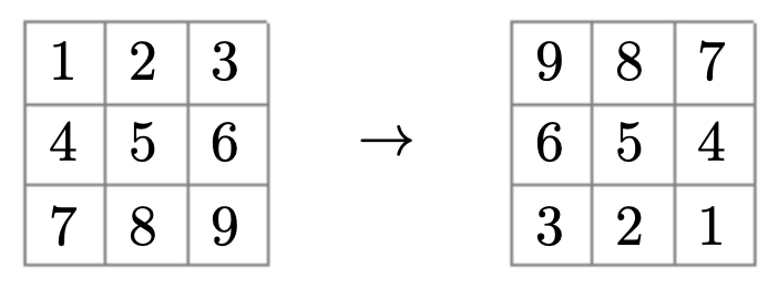
• The following figure illustrates the distinction clearly. On the left, convolution flips the kernel before applying it; on the right, cross-correlation applies the kernel directly. This visualization explains why deep learning libraries prefer cross-correlation: it avoids flipping overhead, and because kernels are learned, the orientation convention is immaterial.

Implications

1. Terminological mismatch: In deep learning, “convolutional neural network” is a misnomer, since the operation is usually cross-correlation. This mismatch can confuse readers comparing CNN literature with classical DSP texts.

2. Fourier domain: True convolution corresponds to multiplication in the Fourier domain, while cross-correlation corresponds to multiplication with the conjugated spectrum of the filter. This distinction is important for theoretical analysis, but not for training CNNs, since kernels are not pre-specified.

3. Implementation: Cross-correlation is slightly more efficient computationally, since it avoids flipping the kernel. As a result, nearly all deep learning libraries adopt it as the primitive operator, even though they still label it “convolution.”

Practical takeaway

• Whether we call it convolution or cross-correlation, the operator serves the same purpose in CNNs: applying local, learnable filters across an input to produce feature maps. The learned nature of the filters means the network adapts to the chosen convention automatically. For all practical purposes in CNNs, “convolution” can be read as “cross-correlation.”

Convolutions over Volume

• Up to this point, we have treated images as 2D arrays of pixel intensities, which works for grayscale images. However, real-world images are usually multi-channel (e.g., RGB with three channels, hyperspectral images with dozens of channels, or feature maps in deeper CNN layers with hundreds of channels). To handle these, the convolution operator is generalized from 2D to 3D volumes. This extension is what allows CNNs to model cross-channel correlations as well as spatial patterns.

Convolution with channels

• Let the input be \(I \in \mathbb{R}^{n_h \times n_w \times n_c}\), where \(n_h\) and \(n_w\) are spatial dimensions and \(n_c\) is the number of channels. A convolutional filter for such an input must span all channels simultaneously. Specifically, each filter has shape \(f \times f \times n_c\), where \(f\) is the spatial size.

• At each spatial location, the filter computes:

• This means that every output value depends not only on the local neighborhood in space but also on all channels of the input. For RGB images, the filter integrates information from red, green, and blue components simultaneously, enabling detectors such as “red-green contrast edges” or “blue-dominant texture.”

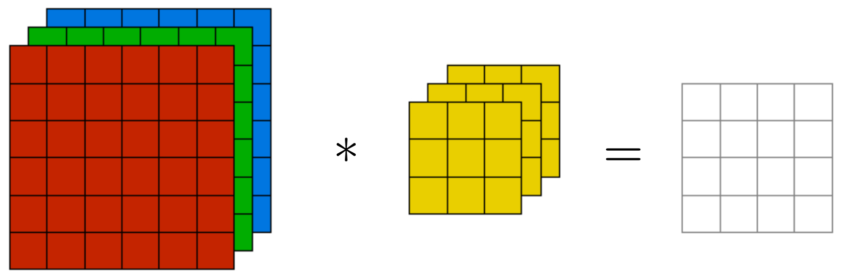
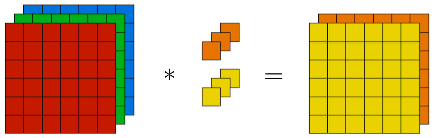
• The following figure visualizes this process: the filter is shown as three stacked slices (one per channel), each interacting with the corresponding channel of the image. Their responses are summed to form a single scalar activation. This highlights that convolution is not independent per channel; instead, it fuses them into a joint response.

Multiple filters and feature maps

• In practice, CNNs do not use just one filter but a bank of filters, each trained to detect a different pattern. If we apply \(n_c'\) filters, the output volume is:

  \[\text{Output size: } n_h^{\text{out}} \times n_w^{\text{out}} \times n_c',\]
  • where \(n_c'\) is the number of filters. Each slice of the output volume corresponds to the response map of one filter.

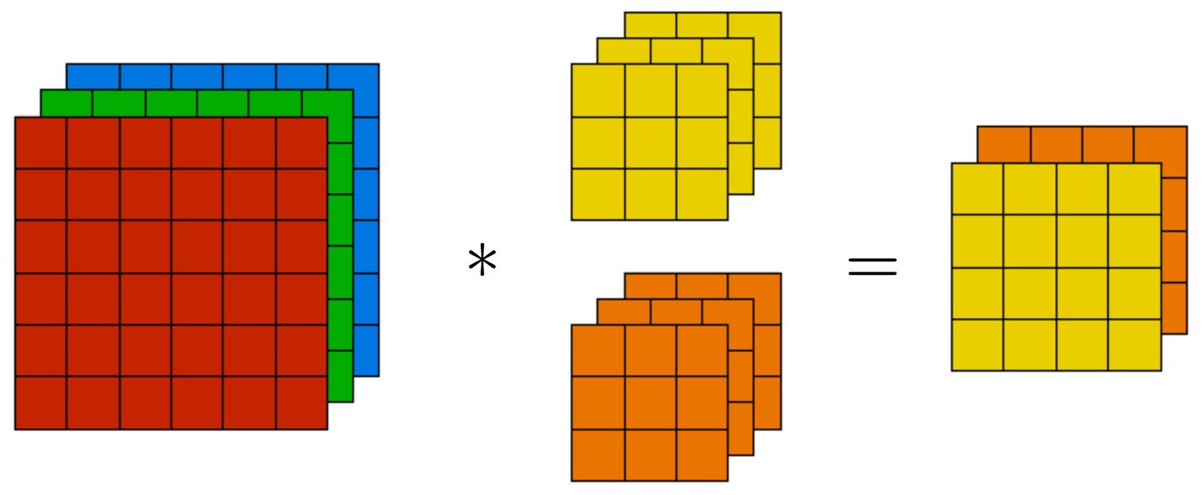
• The following figure illustrates this stacking: each filter produces its own 2D feature map, and the collection of these maps forms the depth of the output tensor. This structure lets CNNs represent an image in terms of many simultaneously detected attributes.

Interpretation

1. Channel mixing. By spanning all input channels, filters learn cross-channel patterns (e.g., color contrasts or combinations of texture and color).
2. Depth as features. The number of filters \(n_c'\) determines the feature depth of the representation. Early CNN layers may have tens of filters, while deep layers in modern networks use hundreds or thousands.
3. Hierarchical abstraction. In shallow layers, filters capture primitive structures (edges, color blobs). In deeper layers, they capture textures, object parts, and even semantic regions (Krizhevsky et al., 2012).

Computational cost

• For a single filter, the parameter count is \(f \times f \times n_c\). With \(n_c'\) filters, the total number of parameters is:

• Each output activation requires \(O(f^2 \cdot n_c)\) multiply–adds. As \(n_c\) grows in deeper layers, the cost increases rapidly, motivating architectural innovations like \(1 \times 1\) convolutions and depthwise separable convolutions.

One-Layer Convolutional Network

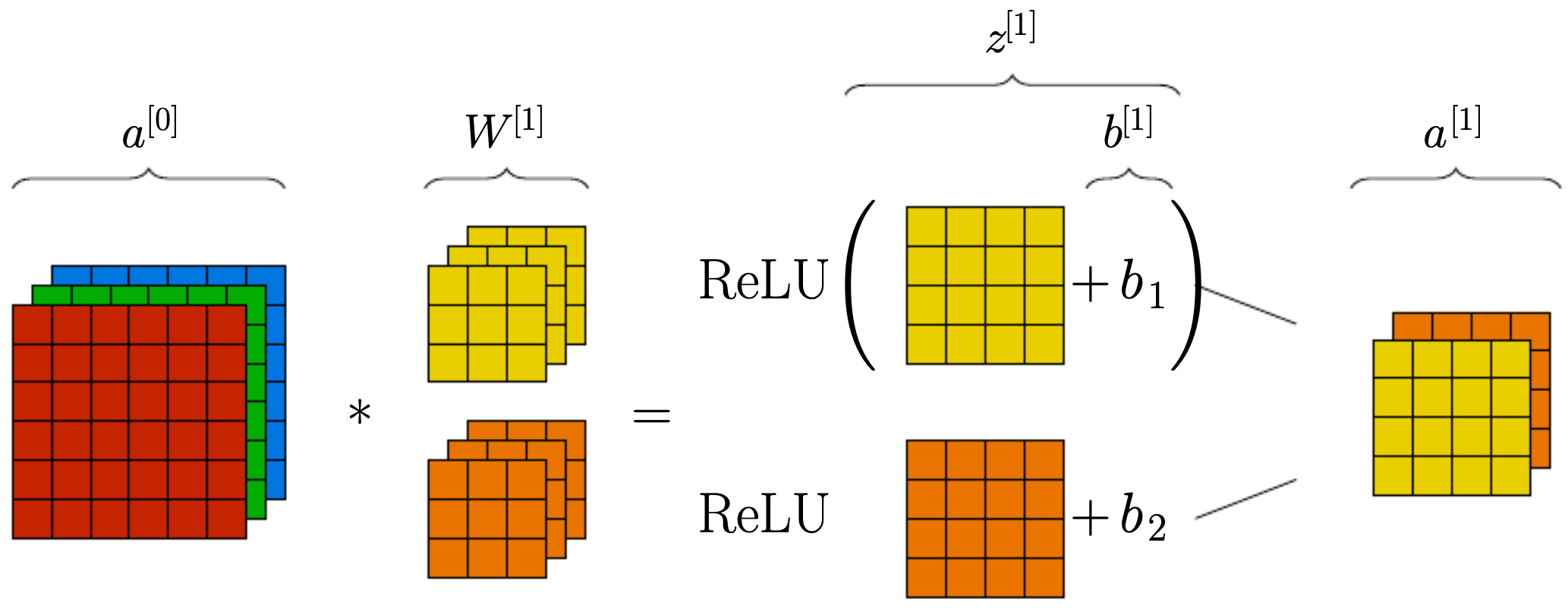
• Having defined convolutions over volumes, we now situate them within the neural network framework. A convolutional layer is more than just convolution: it combines linear convolution with bias terms and non-linear activation functions. This composition forms the fundamental computational block of convolutional neural networks (CNNs). Even with a single convolutional layer, we obtain a model that can detect meaningful features such as edges, corners, and color contrasts across the image.

Linear activation (pre-activation stage)

• For each filter \(W^{[l]} \in \mathbb{R}^{f \times f \times n_c^{[l-1]}}\) at layer \(l\), the pre-activation at a spatial location \((i,j)\) in output channel \(c'\) is:

  \[z^{[l]}(i,j,c') = \sum_{c=1}^{n_c^{[l-1]}} \sum_{u=0}^{f-1} \sum_{v=0}^{f-1} a^{[l-1]}(i+u, j+v, c)\, W^{[l]}(u,v,c,c') + b^{[l]}(c'),\]

  • where:

    • \(a^{[l-1]}\) is the activation volume from the previous layer,

    • \(W^{[l]}\) contains the learnable filter weights,

    • \(b^{[l]}(c')\) is the bias term associated with filter \(c'\),

    • \(z^{[l]}(i,j,c')\) is the scalar linear activation before nonlinearity.

• This equation captures the multiply–accumulate nature of convolution: a weighted sum over the receptive field plus a bias.

Non-linear activation (post-activation stage)

• To enable the network to model non-linear mappings, the pre-activation is passed through an elementwise non-linearity \(g(\cdot)\). A common choice is the Rectified Linear Unit (ReLU):

• The output volume of the convolutional layer is thus

  \[n_h^{[l]} \times n_w^{[l]} \times n_c^{[l]},\]
  • where \(n_c^{[l]}\) is the number of filters. Each channel corresponds to the activation map of a single filter.

• The following figure illustrates this full forward pass. It shows the input being processed by multiple filters, bias terms being added, and ReLU applied, yielding feature maps that already capture edges and textures. This makes clear how even one layer transforms raw pixels into structured information.

Dimensions recap

• For layer \(l\):

  • Filter size: \(f^{[l]}\)
  • Padding: \(p^{[l]}\)
  • Stride: \(s^{[l]}\)
  • Number of filters: \(n_c^{[l]}\)

• If the input has size \(n_h^{[l-1]} \times n_w^{[l-1]} \times n_c^{[l-1]}\), then the output size is:

  \[n_h^{[l]} = \left\lfloor \frac{n_h^{[l-1]} + 2p^{[l]} - f^{[l]}}{s^{[l]}} \right\rfloor + 1,\] \[n_w^{[l]} = \left\lfloor \frac{n_w^{[l-1]} + 2p^{[l]} - f^{[l]}}{s^{[l]}} \right\rfloor + 1,\] \[n_c^{[l]} = \text{number of filters}.\]

Parameter count

• The total number of learnable parameters in layer \(l\) is:

  \[\underbrace{f^{[l]} \times f^{[l]} \times n_c^{[l-1]}}_{\text{weights per filter}} \times n_c^{[l]} + n_c^{[l]} \quad \text{(bias terms)}.\]

• This parameter count is typically much smaller than that of a fully connected layer with comparable input size, since filters are small and shared across spatial positions.

Intuition

• Feature detectors. Each filter acts like a detector for a specific visual pattern. For example, one filter may respond to vertical edges, another to diagonal textures, and another to red–blue contrasts.
• Parameter sharing. The same filter is applied across the whole image, so the same feature can be detected anywhere. This is what gives CNNs translation invariance.
• Sparse connectivity. Each activation depends only on a local neighborhood (the receptive field), which mirrors the locality of natural images.

Pooling Layers

• Pooling layers play a crucial role in convolutional neural networks (CNNs). While convolutional layers are responsible for extracting features, pooling layers are responsible for compressing those features in a way that reduces redundancy, improves efficiency, and increases robustness to small spatial variations. Importantly, pooling layers contain no learnable parameters—they apply a deterministic aggregation function over local neighborhoods.

• Intuitively, pooling asks: instead of keeping every fine-grained response from convolution, can we summarize each small region with a single representative value? This mirrors the way human vision focuses on salient information while ignoring unnecessary detail.

Mechanics of pooling

• A pooling layer is defined by two hyperparameters:

  • Filter size \(f\): the spatial extent of the pooling window (e.g., \(f=2\)).
  • Stride \(s\): how far the pooling window moves across the input.

• For each \(f \times f\) window in the input, pooling computes a single summary statistic, producing a downsampled feature map.

• Two main pooling functions are widely used:

  1. Max pooling
  \[a^{[l]}(i,j,c) = \max_{(u,v) \in f \times f} a^{[l-1]}(s i + u, \, s j + v, \, c).\]
  • Retains only the strongest activation in the window.
  • Acts as a detector: “Did this feature appear in this region?”
  1. Average pooling
  \[a^{[l]}(i,j,c) = \frac{1}{f^2} \sum_{(u,v) \in f \times f} a^{[l-1]}(s i + u, \, s j + v, \, c).\]

  • Computes the average intensity of the activations in the window.

  • Captures the overall presence of features, but can blur strong signals.

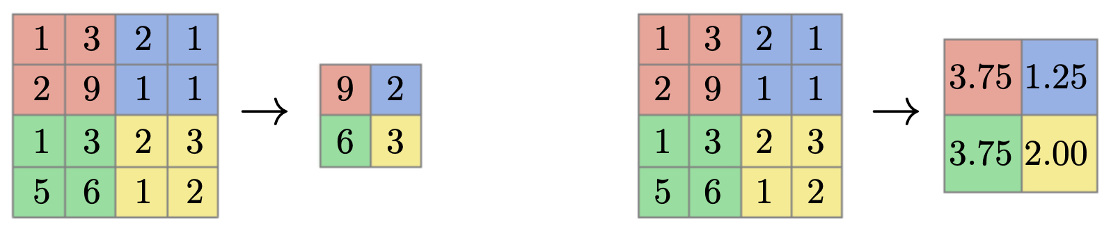
• The following figure compares max pooling (left) and average pooling (right) on a toy 2D input with \(f=2\) and \(s=2\). Notice how max pooling preserves sharp signals by picking the strongest activation, while average pooling smooths the activations.

Intuition

• Max pooling is like asking “is there a strong feature anywhere in this region?” It keeps discriminative cues intact.
• Average pooling is like asking “what is the overall level of activation in this region?” It smooths details but may lose sharpness.
• Empirically, max pooling tends to perform better in classification settings because it preserves salient patterns.

3D pooling (multi-channel inputs)

• For input volumes with multiple channels, pooling is applied independently to each channel. This means that while height and width are reduced, the number of channels remains unchanged:

• Thus, pooling preserves the depth structure of the representation while compressing its spatial footprint.

Advantages of pooling

1. Dimensionality reduction. Shrinks feature maps, reducing the computational cost of later layers.
2. Translation invariance. A small shift in the input produces the same pooled output, making the network more robust.
3. No parameters. Pooling is a fixed operation—simple and efficient.
4. Hierarchical abstraction. By compressing details, pooling allows deeper layers to focus on more abstract patterns (e.g., object parts rather than edges).

Modern perspective

• In early CNNs such as LeNet, AlexNet, and VGG, pooling was a dominant tool for downsampling.
• In more recent architectures (e.g., ResNets, DenseNets, Transformers), strided convolutions are often used instead of pooling, since they combine feature extraction and downsampling in a single learnable operation.
• Nevertheless, pooling remains conceptually important, and some architectures still use it selectively, especially where robustness to small distortions is critical.

Why We Use Convolutions

• To fully understand the motivation for convolutional neural networks (CNNs), it helps to compare them with the naïve baseline: applying fully connected (dense) networks directly to raw image pixels. At first glance, one might flatten an image into a 1D vector and feed it into a dense layer. While this approach is mathematically valid, it quickly becomes computationally infeasible and statistically inefficient as image sizes increase.

• Convolutions solve these problems by exploiting the spatial structure of images, introducing two powerful principles: parameter sharing and sparse connectivity. Together, these allow CNNs to scale to high-resolution inputs, generalize better, and use far fewer parameters than dense layers.

Fully connected baseline

• Consider an image of size \(32 \times 32 \times 3\) (height × width × channels). Flattening yields a vector of length

• Suppose we want to map this input to an output volume of size \(28 \times 28 \times 6 = 4704\). A fully connected layer would require a weight matrix with

• Such a network is not only computationally expensive but also highly prone to overfitting, since it tries to learn too many parameters relative to typical dataset sizes.

Convolutional alternative

• Instead, let’s replace the dense mapping with a convolutional layer using:

  • Filter size \(f = 5 \times 5\),
  • Input depth \(n_c = 3\),
  • Number of filters \(n_c' = 6\).

• The total number of parameters is:

  \[5 \times 5 \times 3 \times 6 = 450 \quad \text{weights},\]
  • plus 6 bias terms.

• That is a reduction from 14.5 million down to 456 parameters — a difference of four orders of magnitude. This massive efficiency gain is what makes deep CNNs feasible.

Two key ideas

1. Parameter sharing

   • A filter is applied across the entire image, using the same set of weights at every spatial location.
   • This drastically reduces the number of parameters and ensures that the same pattern (e.g., a vertical edge) can be recognized anywhere in the image.

2. Sparsity of connections

   • Each output value depends only on a local neighborhood (the receptive field), rather than the entire image.
   • This reflects the natural statistics of images, where nearby pixels are highly correlated, while distant ones are less so.
   • Sparse connectivity makes learning more efficient and emphasizes local-to-global feature hierarchies.

Implications

• Statistical efficiency: With far fewer parameters, CNNs require fewer training examples to generalize effectively.
• Generalization: Learned features are position-invariant — the same filter can detect a pattern regardless of where it appears.
• Scalability: Convolutions enable networks to handle large, high-resolution images without exploding parameter counts.
• Inductive bias: CNNs embed assumptions about locality and translational invariance, which align well with the structure of natural images.

Classic Networks

• While the principles of convolution, pooling, and nonlinearities define the building blocks of CNNs, much of the field’s progress has come from architectural design breakthroughs. Over the years, several networks have become landmark architectures, each introducing innovations that pushed performance forward on benchmark datasets and inspired future designs. In this section, we review some of the most influential CNNs: LeNet-5, AlexNet, VGG-16, ResNet, and Inception (GoogLeNet).

LeNet-5

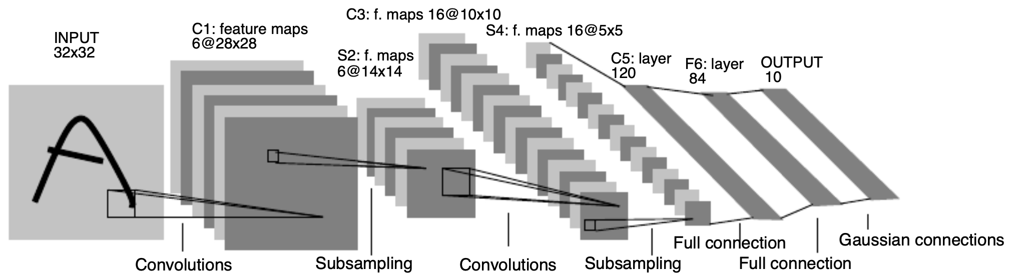
• Introduced by LeCun et al., 1998, LeNet-5 is one of the earliest CNNs, originally designed for handwritten digit recognition (e.g., MNIST).

• Architecture: A sequence of convolutional and subsampling (average pooling) layers, followed by fully connected layers.

• Parameter count: ~60,000 learnable parameters — tiny by today’s standards.

• Key idea: Progressively increase the number of feature maps while reducing spatial resolution, so deeper layers capture more abstract features.

• Impact: Demonstrated the feasibility of CNNs for real-world vision tasks long before GPUs and large datasets were available.

• The following figure shows the original LeNet-5 architecture, highlighting how feature extraction (via convolutions) and dimensionality reduction (via pooling) lead to compact representations that feed into dense classification layers.

AlexNet

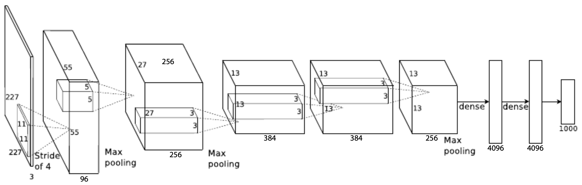
• AlexNet, introduced by Krizhevsky et al., 2012, marked the deep learning revolution by winning the 2012 ImageNet competition with a massive performance gap over traditional methods.

• Architecture: Similar in spirit to LeNet, but much deeper, with 5 convolutional layers and 3 fully connected layers.

• Parameter count: ~60 million.

• Key innovations:

  • ReLU activation function (faster convergence than sigmoid/tanh).
  • GPU training to scale computation.
  • Dropout for regularization.
  • Data augmentation to improve generalization.

• Impact: Sparked a surge of research in deep learning and cemented CNNs as the standard for computer vision.

• The figure below illustrates the AlexNet architecture: stacked convolutional and pooling layers feeding into large fully connected layers. It also shows how the model was distributed across two GPUs for training, an engineering trick that was critical at the time.

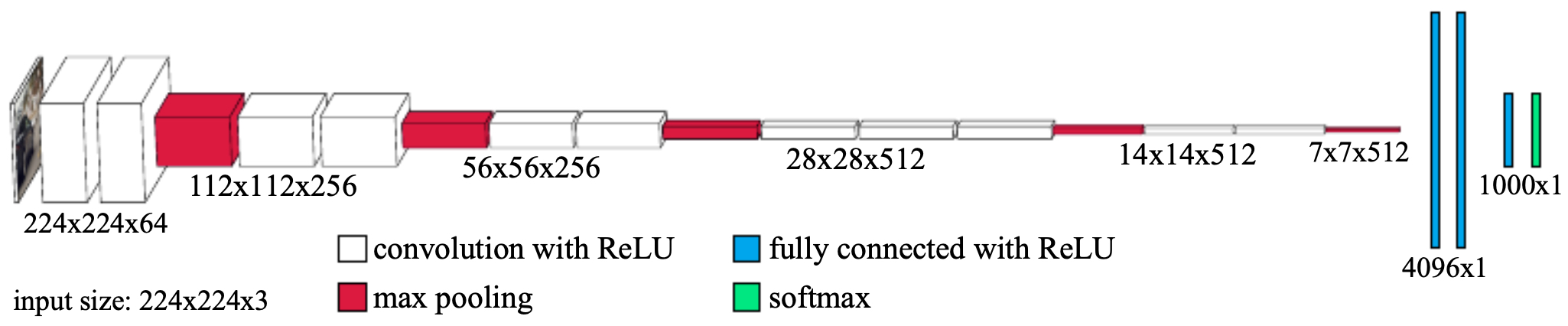
VGG-16

• Introduced by Simonyan & Zisserman, 2015, VGG-16 became highly influential due to its simplicity and depth.

• Architecture: 16 layers deep, using only \(3 \times 3\) convolutions with stride 1 and \(2 \times 2\) max pooling with stride 2.

• Parameter count: ~138 million — very large at the time.

• Key insight: Stacking small filters (e.g., \(3 \times 3\)) can approximate larger receptive fields (e.g., \(5 \times 5\), \(7 \times 7\)) while reducing parameters and improving generalization.

• Impact: Its clean, uniform design made it a standard backbone for many applications (e.g., object detection, style transfer).

• The following figure shows the VGG-16 pipeline: input → repeated \(3 \times 3\) convolutions → pooling → dense layers. The uniformity of this structure made it both powerful and easy to adapt.

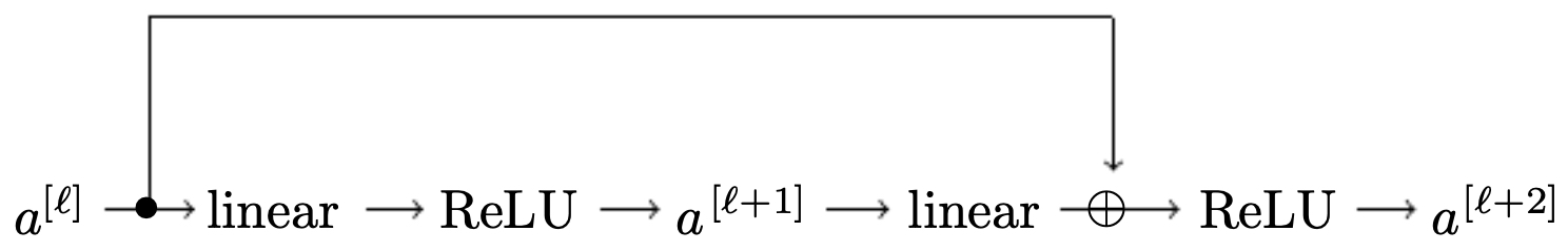
ResNet

• Residual Networks (ResNets), introduced by He et al., 2015, solved the training degradation problem: as networks grew deeper, adding more layers led to higher training error, not just overfitting.

• Solution: Add skip connections (identity mappings) that let information and gradients flow across layers.

• Residual block:

  \[a^{[l+2]} = g(z^{[l+2]} + a^{[l]}),\]
  • where the input is added directly to the output of two stacked layers.

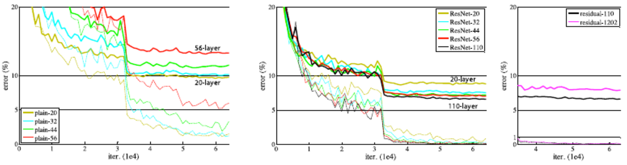
• Impact: Enabled the training of extremely deep networks (50, 101, 152 layers and beyond), achieving state-of-the-art results on ImageNet and other benchmarks.

• The next figure illustrates a residual block, where the shortcut bypasses two convolutional layers, preserving gradient flow.

• The following plots compare error rates: “plain” deep networks degrade as depth increases, while ResNets continue to improve, demonstrating scalability.

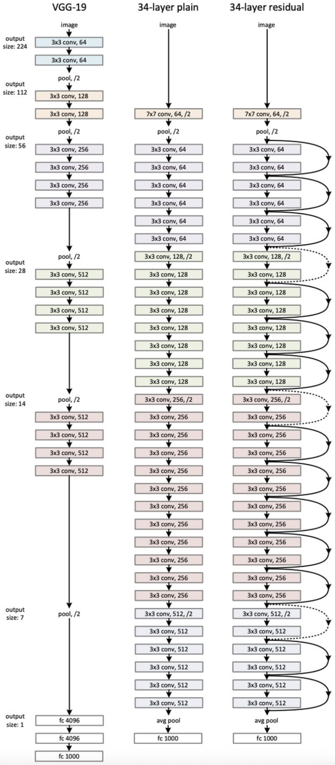
• Another figure compares ResNet-34 against plain networks and VGG-19, showing ResNets outperform both deeper and shallower alternatives.

1×1 Convolution

• A \(1 \times 1\) convolution may seem trivial, but in multi-channel inputs it is highly useful:

  • Each filter spans all channels but only one spatial location.
  • Outputs are linear combinations of channels, enabling dimensionality reduction or expansion.
  • This reduces parameter counts and accelerates computation while preserving expressivity.

• Often called “Network-in-Network,” this idea was popularized by Lin et al., 2013.

• The figure below shows how \(1 \times 1\) filters recombine channels at each spatial location, acting as a learnable projection.

Inception Network (GoogLeNet)

• Introduced by Szegedy et al., 2015, the Inception architecture (GoogLeNet) aimed to let the model adaptively choose receptive field sizes instead of fixing them by hand.

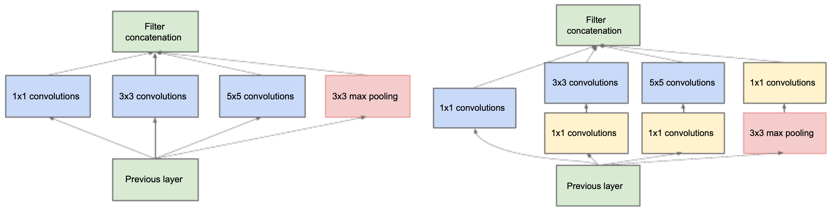
• Key idea: Apply multiple filter sizes (\(1 \times 1\), \(3 \times 3\), \(5 \times 5\)) and max pooling in parallel, then concatenate their outputs.

• Challenge: Larger filters (e.g., \(5 \times 5\)) are expensive.

• Solution: Precede them with \(1 \times 1\) convolutions to reduce channel dimensionality, making the module efficient.

• Impact: Provided a flexible, efficient building block that became the basis of many modern CNNs.

• The following figures illustrate inception modules: (Left) the naïve version applies all filters directly, while (Right) the improved design uses \(1 \times 1\) reductions before larger filters.

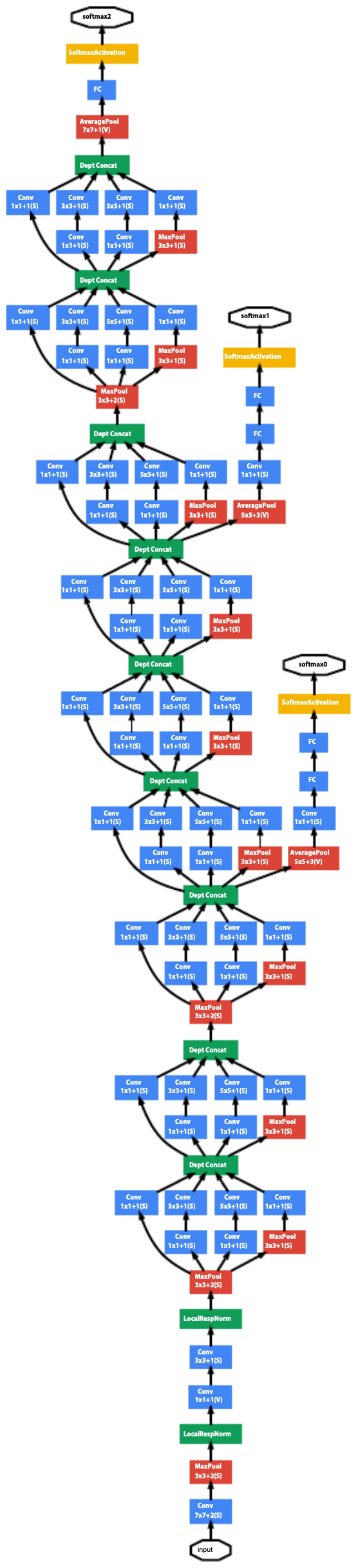
• The full GoogLeNet architecture is a stack of such modules, forming a deep yet efficient network.

• As a humorous aside, the authors cited a meme (from the film Inception) as inspiration for the network’s name.

Summary of classic networks

• LeNet-5: Proved CNNs could work in practice (digits).
• AlexNet: Sparked the deep learning revolution (ImageNet 2012).
• VGG-16: Showed that deep, uniform architectures with small filters are powerful.
• ResNet: Solved the vanishing gradient problem with skip connections, enabling ultra-deep networks.

• Inception: Innovated with multi-scale filters and \(1 \times 1\) dimensionality reduction.

• Together, these architectures established the design principles that continue to shape modern CNNs.

Competitions and Benchmarks

• The rapid evolution of convolutional neural networks (CNNs) has been tightly coupled with the availability of large-scale benchmarks and competitions. These resources provided standardized datasets, objective evaluation metrics, and community-wide challenges that motivated researchers to push architectures forward. Among them, the ImageNet Large Scale Visual Recognition Challenge (ILSVRC) stands out as the single most influential benchmark in shaping modern deep learning.

Benchmark-driven progress

• ImageNet (ILSVRC, 2010–2017)

  • Dataset: 1.2 million training images, 50,000 validation images, 100,000 test images, and 1,000 object classes.
  • Significance: First large-scale, diverse dataset enabling deep models to show their potential beyond toy problems like MNIST or CIFAR.
  • Metric: Top-1 and Top-5 error rates (how often the correct label is the highest-probability prediction, or within the top 5).

• CNN breakthroughs on ImageNet:

  • AlexNet (2012) cut error rates by ~10 percentage points compared to the best traditional methods.
  • VGG (2014) showed that simply making networks deeper improved performance.
  • GoogLeNet (2014) introduced Inception modules, balancing accuracy and efficiency.
  • ResNet (2015) achieved human-level accuracy by enabling training of 100+ layer models.

• Other benchmarks also played key roles:

  • CIFAR-10/100 (small images, 10 or 100 classes) — used to prototype new ideas.
  • Pascal VOC — focused on object detection.
  • COCO — enabled benchmarking for dense tasks such as detection and segmentation.

• These datasets together fostered a culture of public leaderboards, which accelerated competition and innovation.

Test-time strategies

• To climb leaderboard rankings, researchers employed test-time enhancements that improved accuracy but were rarely used in production due to high cost. Two main strategies stand out:

1. Ensembling

   • Train multiple CNNs (often 3–15 models) with different initializations or architectures.
   • At test time, average their predictions (for regression) or use majority voting (for classification).
   • Boosts accuracy, but multiplies inference cost and memory footprint proportionally to the number of models.

2. Multi-crop evaluation

   • Instead of testing on a single crop (e.g., center), generate multiple views of the image: corners, center, and their mirrored counterparts.
   • Each crop is passed through the network, and the predictions are averaged.
   • Reduces sensitivity to image position and cropping, improving robustness at the cost of more compute.

• The figure below illustrates the 10-crop technique: one center crop, four corner crops, and their mirrored versions. These 10 inputs are each passed through the CNN, and the results are averaged. This improves accuracy by smoothing out viewpoint biases, but inference is 10× slower.

Practical considerations

• While ensembling and multi-crop evaluations helped win competitions, they are computationally prohibitive for real-world systems where latency and efficiency are critical. Instead, practitioners prefer:

  1. Single, optimized models — trained with aggressive data augmentation so they generalize well without multi-crop testing.
  2. Model compression and pruning — to reduce inference time and memory cost.
  3. Quantization — lowering weight precision (e.g., FP32 → INT8) for faster hardware execution.
  4. Knowledge distillation — training a smaller “student” model to mimic a large ensemble “teacher.”

• Thus, competition-driven tricks inspired ideas that later translated into practical deployment strategies, even if the raw techniques themselves (ensembles, multi-crop) are rarely used in production.

Citation

If you found our work useful, please cite it as:

@article{Chadha2020CNNs,
  title   = {Convolutional Neural Networks},
  author  = {Chadha, Aman},
  journal = {Distilled Notes for Stanford CS230: Deep Learning},
  year    = {2020},
  note    = {\url{https://aman.ai}}
}